Missing Data Imputation for Geolocation-based Price Prediction Using KNN–MCF Method

Abstract

Accurate house price forecasts are very important for formulating national economic policies. In this paper, we offer an effective method to predict houses’ sale prices. Our algorithm includes one-hot encoding to convert text data into numeric data, feature correlation to select only the most correlated variables, and a technique to overcome the missing data. Our approach is an effective way to handle missing data in large datasets with the K-nearest neighbor algorithm based on the most correlated features (KNN–MCF). As far as we are concerned, there has been no previous research that has focused on important features dealing with missing observations. Compared to the typical machine learning prediction algorithms, the prediction accuracy of the proposed method is 92.01% with the random forest algorithm, which is more efficient than the other methods.

1. Introduction

Real estate property is one of the main necessities of human beings. Additionally, these days it demonstrates the affluence and status of an individual. Savings in property is commonly lucrative because its worth does not decline immediately. Instabilities in the property prices can impact several household stockholders, financiers, and policy makers. Furthermore, the majority of investors prefer to invest in the real sector. Therefore, predicting the cost of real estate is an imperative economic index. To predict the house price, we need a good organized dataset from real estates. In this work, we used a publicly available dataset from Kaggle Inc. [1]. It contains 3000 training examples with 80 features that influence the real estate prices. However, data preprocessing techniques such as one-hot encoding, feature correlation, and the handling of missing data must be applied to obtain a good result.

One-hot encoding is the most widely used binary encoding method to convert text data into numeric data [2]. Selection of features reduces the feature space dimensionality and removes unnecessary, unconnected, or noisy data. It has the following instant impact on a prediction: data quality improvement, machine learning (ML) process’s acceleration, and increase of the comprehensibility of the prediction [3,4]. In addition to the above-mentioned preprocessing problems, missing data are a problem, as almost all the ordinary statistical approaches assume complete information for all the attributes belonging to the examination. Comparatively few vague observations on some variables can considerably decrease the sample size. Accordingly, the accuracy of confidence is damaged, statistical power fades, and the parameter evaluations may be influenced [5].

In our approach, we used the KNN-based most correlated features (KNN–MCF) algorithm for dealing with the missing data. The main idea was to use only the most meaningful variables found using a simulation, for handling the absent data with the KNN algorithm. In this advanced method, the accuracy of the house price prediction is distinctly better than that of the traditional ways of handling missing data, such as the mean, median, and mode. We compared our method with the traditional mean and KNN methods by implementing them on several machine learning algorithms.

The organization of the rest of this paper is as follows: the related works are discussed in Section 2. Section 3 contains the dataset and methods used in this work. Section 4 demonstrates the results, and Section 5 finishes this paper with the conclusions and a brief discussion of future work directions.

2. Related Works

We reviewed some related works that attempted to predict house prices with the data preprocessing techniques explored in this section. We examined what has been done and what can be learnt from these efforts. A more thorough discussion of the missing data methods can be found in [6,7]. Missing or incomplete data are a common drawback for a lot of real-world cases in pattern classification [8,9,10]. In [11], the author has enumerated the most macroeconomic parameters that influence the fluctuation of house prices. In [12], researchers tried to predict the sale price of the houses by utilizing several machine learning techniques. The data in our work and their work are the same. However, the authors used a simple way to avoid the missing data. They just eliminated the observations that had a missing value. This method led to a decrease in the size of the dataset.

The removal of observations can cause evaluations with relatively large average errors because of the reduced sample size [13]. Eliminating rows in the dataset that have missing data yields prejudiced or dissatisfactory consequences even though such techniques are still commonly used in software manufacturing [14]; we know this method as “complete case analysis.” This strategy eliminates some variables that are needed to meet the anticipations essential for satisfactory clarifications [13]. In a number of studies, the imputation of numerical data missing values have been regularly dealt with using the mean replacement [14]. The primary negative point is that this strategy can change the distribution for the attribute that is used for imputation by misjudging the standard deviation [15]. Furthermore, median imputation is executed to boost durability, since the outliers of the dataset may influence the mean value. The mode imputation is generally used for categorical features instead of the mean imputation and the median imputation [16].

The downside of this method is that it cannot handle the dependencies between the feature values [7]. Additionally, the paper [17] discussed the test dataset with some missing data and selected diverse missing percentage values in their work. Mean, median, and standard deviation were assigned for each value. They yielded different results for every case. In [5], missing data mechanisms and patterns of missing data have been explained well. The authors of this article considered some advanced techniques for handling missing data, like maximum likelihood as well as multiple imputation. According to [18], we can list two important features of the KNN method: the KNN impute function can effortlessly deal with and predict both quantitative and qualitative attributes, and this method can directly handle a number of missing values. Even though KNN impute has been widely used for dealing with missing data, there are some downsides [19,20,21] when it is executed on a large dataset [15].

In order to compare our method with the current techniques, firstly, we employed a simple method, the mean of all the non-missing observations, to handle the missing data. The main disadvantage of this method is that all the missing data were filled with the same mean value [22]. Therefore, this method is not widely used in the field of data science now. The second method that we used to impute the missing data was the KNN algorithm. In this method, we investigated KNN algorithm’s function to impute the missing values called KNN impute [18]. If there is a partial feature, this technique chooses its K nearest examples from the training samples with the known values in the attributes to be imputed, such that they diminish the distance. After the K closest neighbors have been gained, a substitution value must be evaluated to restore the missing attribute value. The sort of replacement value relies on the kind of the data used—the mean can be used for continuous data and the mode for qualitative data.

Based on the above-mentioned studies, we realized that we can improve the methodology for imputing missing data with the KNN algorithm by choosing the most important features that have a huge impact on the house price prediction. The system architecture obtained using the proposed method is depicted below.

3. Materials and Methods

3.1. Dataset

Our initial dataset was obtained from the Kaggle [23] dataset, which provides data scientists with a huge amount of data to train their machine learning models. It was collected by Bart de Cock in 2011 and is significantly bigger than the well-known Boston housing dataset [24]. It contains 79 expressive variables, which demonstrate almost each feature of residential homes in Ames, Iowa, USA, during the period from 2006 to 2010. The dataset consists of both numeric and text data. The numeric data include information about the number of rooms, size of rooms, and the overall quality of the property. In contrast to numeric data, the text data is provided in words. The location of the house, type of materials used to build the house, and the style of the roof, garage, and fence are the examples of the text data.

Table 1. Data description.

Data Category	Number of Features	Description
Numeric data	36	No. of rooms, size of rooms, date info, quality of house, etc.
Text data	43	Location of house, style of house, etc.

illustrates the description of the dataset.

The main reason for dividing the dataset into different types of data was that the text data had to be converted into numeric data with the one-hot encoding technique before training. We will describe this encoding method in the following data preprocessing section of our methodology. A total of 19 features have missing values out of a total of 80 features. The percentage of missing values is 16%.

3.2. Data Preprocessing

In this process, we transformed raw, complicated data into organized data. This consisted of several procedures from one-hot encoding to finding the missing and unnecessary data in the dataset. Several machine learning techniques can work with categorical data right away. For instance, a decision tree algorithm can operate with categorical data without the need of data transformation. However, numerous machine learning systems cannot work with labeled data. They need all variables (input and output) to be numeric. This can be regarded as a huge limitation of machine learning algorithms rather than hard limitations on the algorithms themselves. Therefore, if we have categorical data then we must convert it into numerical data. There are two common methods to create numeric data from categorical data:

• one-hot encoding
• integer encoding

In the case of the house location, the houses in the dataset may be located in three different cities: New York, Washington, and Texas. The city names need to be converted into numeric data. Firstly, each unique feature value is given an integer value; for instance, 1 is for “New York”, 2 is for “Washington”, and 3 is for “California”. For several attributes, this might be sufficient. This is because integers have an ordered connection with each other, which enables machine learning techniques to comprehend and harness that association. In contrast, categorical variables possess no ordinal relationship; therefore, integer encoding is not able to solve the issue. The use of such encoding and allowing the model to get the natural ordering between categories may have poor application or unanticipated outcomes. We provide the above-mentioned example of a toy dataset in

Table 2. Toy dataset with house ID and its location.

ID	Location
0	New York
1	Washington
2	New York
3	California
4	New York

and its integer encoding in

Table 3. Integer encoding of the toy dataset.

ID	Location
0	1
1	2
2	1
3	3
4	1

. It can be noticed that the ordering between categories results in a less precise prediction of the house price.

In order to solve the problem, we can use one-hot encoding. This is where the integer determined variable is removed and a new binary variable is added for each single integer value [2]. As we mentioned, based on our data, we may face the situation where our model is confused by thinking that a column has the data with a certain order or hierarchy. However, it can be avoided by “one-hot encoding”, in which label encoded categorical data is split into numerous columns. The numbers are substituted by 1s and 0s, based on the values of the columns. In our case, we got three new columns, namely New York, Washington, and California. For the rows that have the first column value as New York, “1” will be assigned to the “New York” column, and the other two columns will get “0”s. Likewise, for rows that have the first column value as Washington, “1” will be assigned to the “Washington”, and the other two columns will have “0” and so on (see

Table 4. One-hot encoding of the toy dataset.

ID	New York	Washington	California
0	1	0	0
1	0	1	0
2	1	0	0
3	0	0	1
4	1	0	0

). We used this type of encoding in the data preprocessing part.

In case of missing values, one-hot encoding converts missing values into zeros. Here is the example shown in

Table 5. Toy dataset with house ID and its location with missing house location information.

ID	Location
0	New York
1	Washington
2	New York
3	NaN
4	California

:

In above-given table, the third value is missing. When converting these categorical values into numeric, all non-missing values have one(s) in their corresponding ID rows. Missing values however, get zeros in respective ID rows. Now we will see the result of how one-hot encoding treats this value.

Thus, the third example gains only zeros as we see in

Table 6. One-hot encoding of the sample dataset given in Table 5.

ID	New York	Washington	California
0	1	0	0
1	0	1	0
2	1	0	0
3	0	0	0
4	0	0	1

. Before selecting most correlated features and dealing with missing values, we convert these zeros again into missing values.

3.3. Feature Correlation

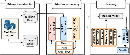
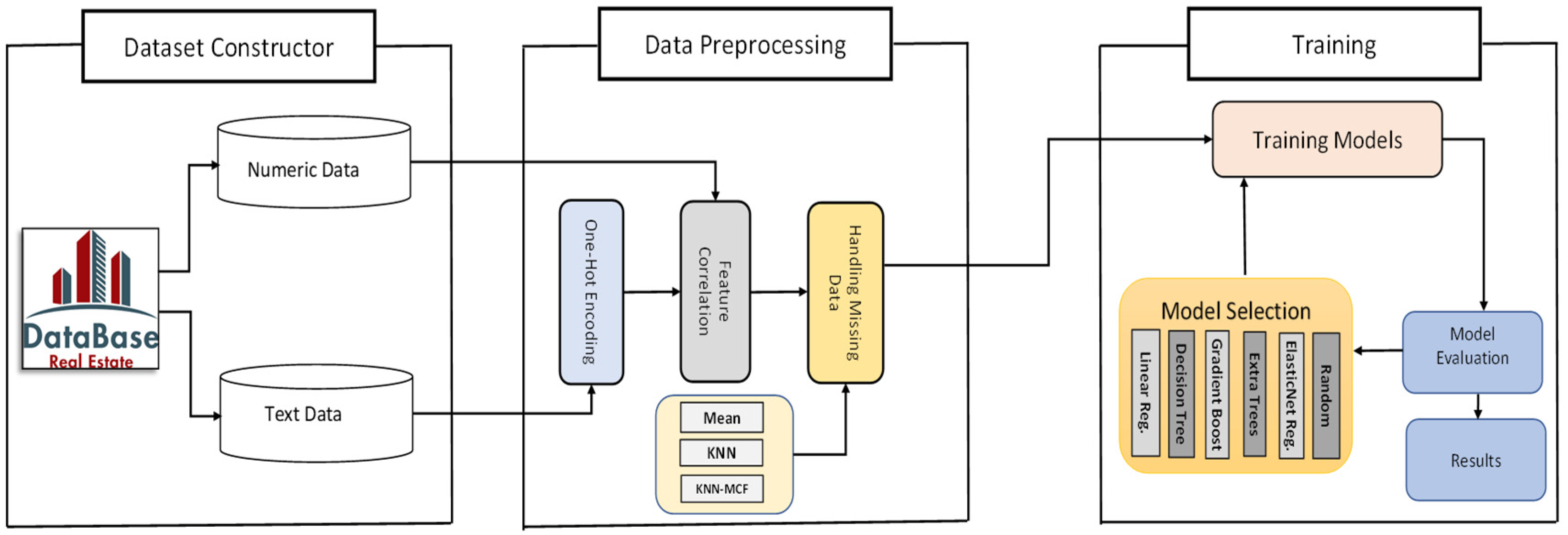
Feature selection is a vigorous sphere in computer science. It has been a productive research area since the 1970s in a number of fields, such as statistical pattern recognition, machine learning, and data mining [25,26,27,28,29,30,31,32]. The central suggestion in this work is to apply feature correlation to the dataset before dealing with the missing data by using the KNN algorithm. By doing so, we can illustrate an optimized K-nearest neighbor algorithm based on the most correlated features for the missing data imputation, namely KNN–MCF. First, we encoded the categorical data into numeric data, as described in the previous subsection. The next and main step was to choose the most important features related to the house prices in the dataset. The overall architecture of the model is illustrated in Figure 1.

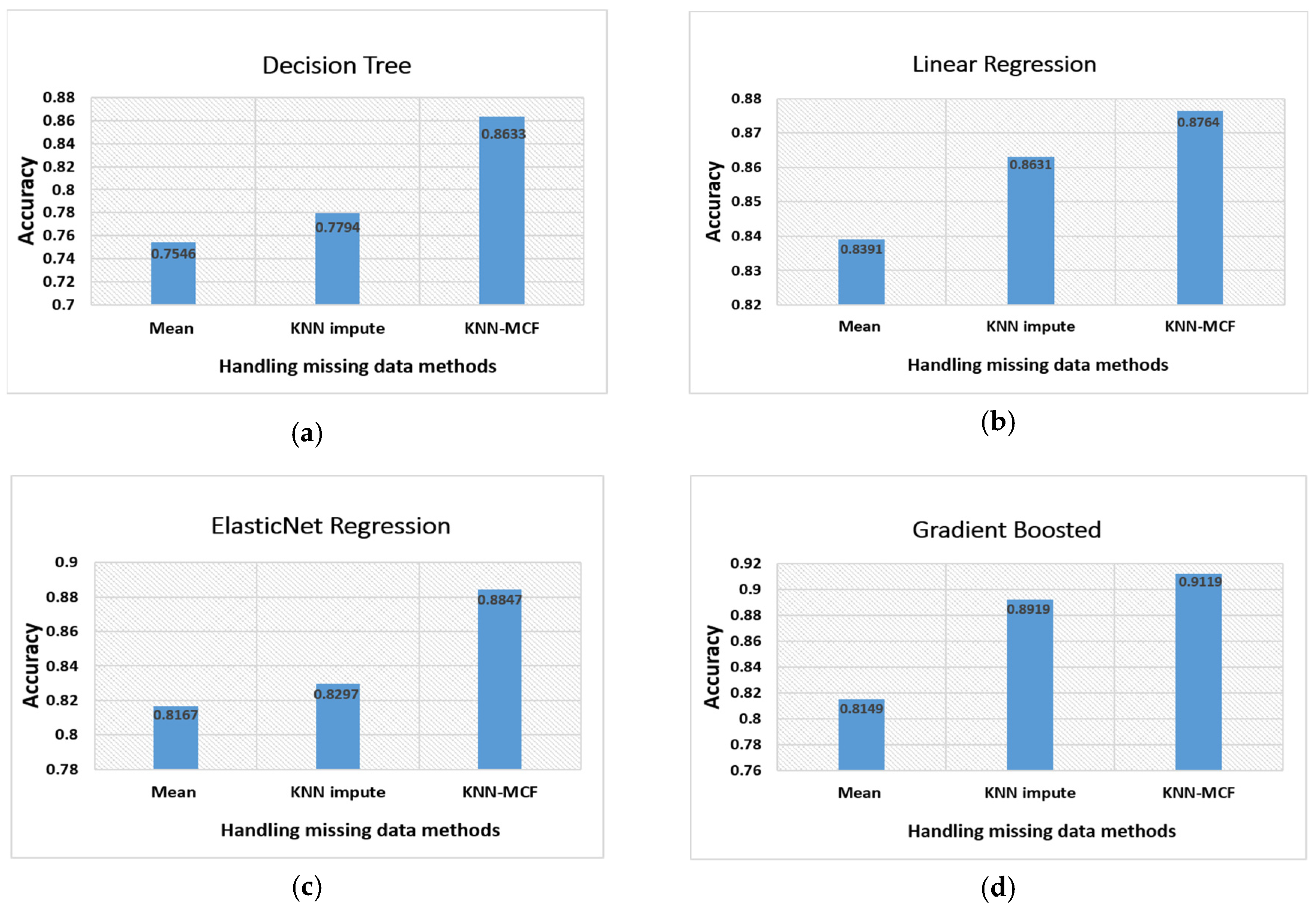
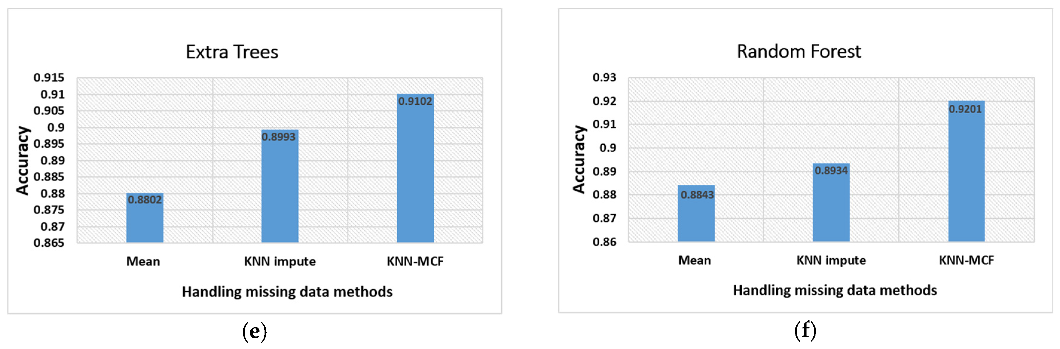
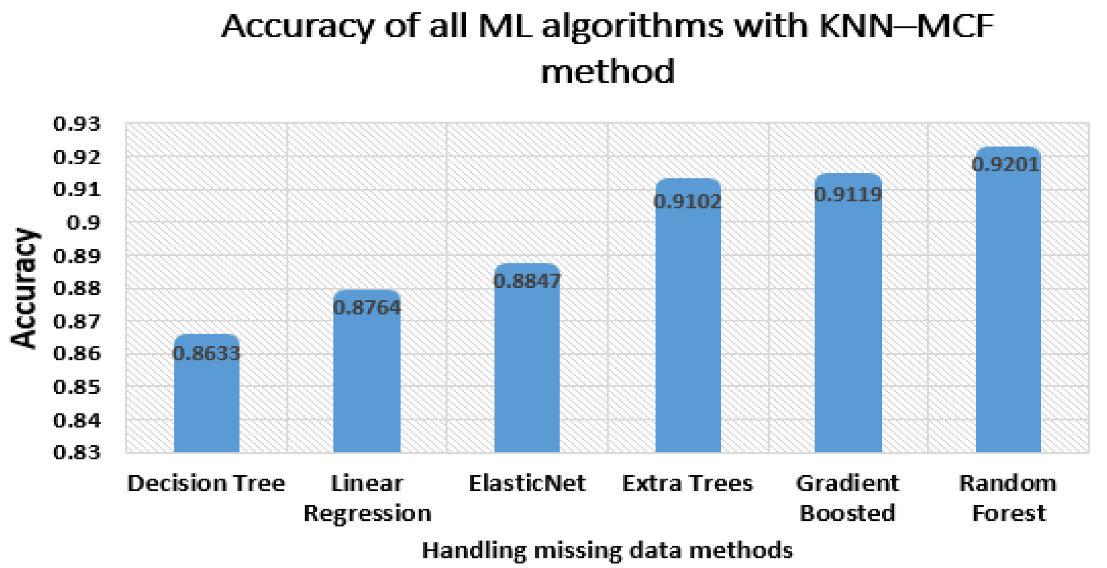
Then, we implemented three methods of handling missing data:

• mean value of all non-missing observations,
• KNN algorithm, and
• KNN–MCF, which is the proposed algorithm for handling the missing data.

The accuracy of each model implemented in the training part improved after the application of the method. Now, we will explain the selection of the most important features. There are different methods for feature correlation. In this work, we used the correlation coefficient method for selecting the most important features. Let us assume that we have two features: a and b. The correlation coefficient between these two variables can be defined as follows:

Correlation coefficient:

$$r\left(a,b\right)=\frac{Cov\left(a,b\right)}{\sqrt{Var\left(a\right)}\sqrt{Var\left(b\right)}}$$

(1)

where, Cov(a, b) is the covariance of a and b and Var(.) is the variance of one feature. The covariance between two features is calculated using the following formula:

$$Cov\left(a,b\right)=\frac{\sum \left(a_{i }– \overline{a}\right)\left(b_i – \overline{b}\right)}{n}$$

(2)

In this formula:

• $a_i$—values of variable “a”
• $\overline{a}$—mean (average) value of variable “a”
• $b_i—$values of variable “b”
• $\overline{b}$—mean (average) value of variable “b”

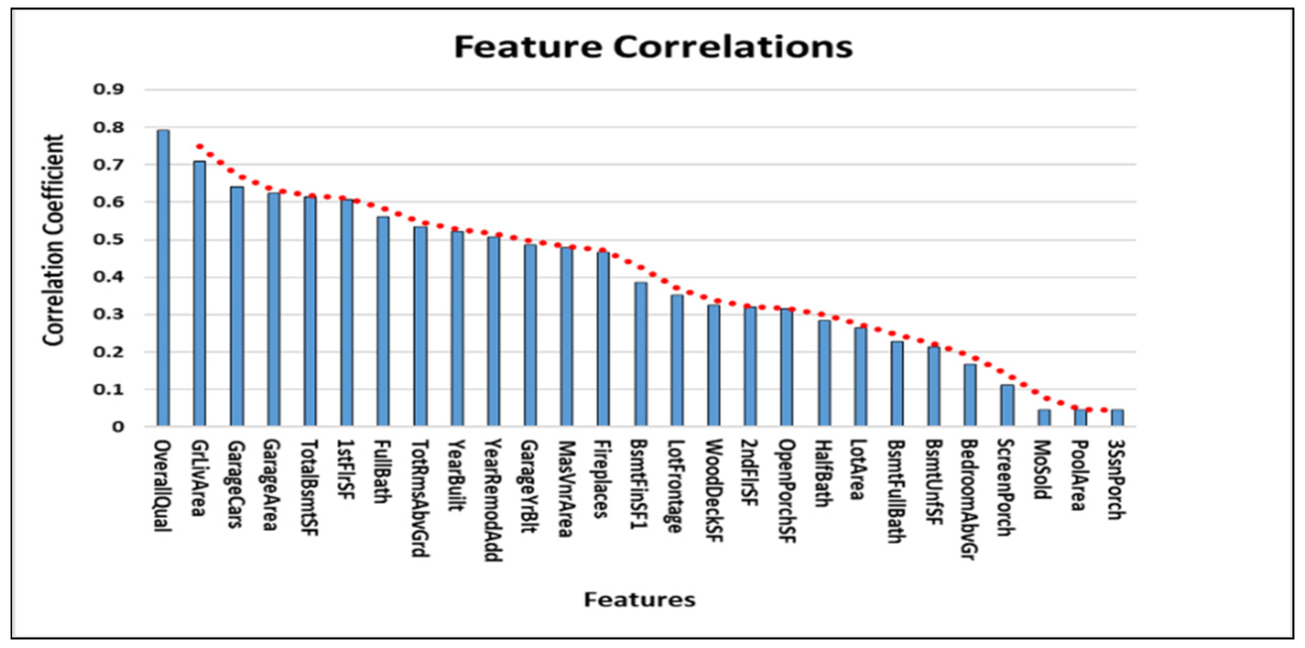
After implementing the above formula into the dataset, we obtained the result illustrated in Figure 2.

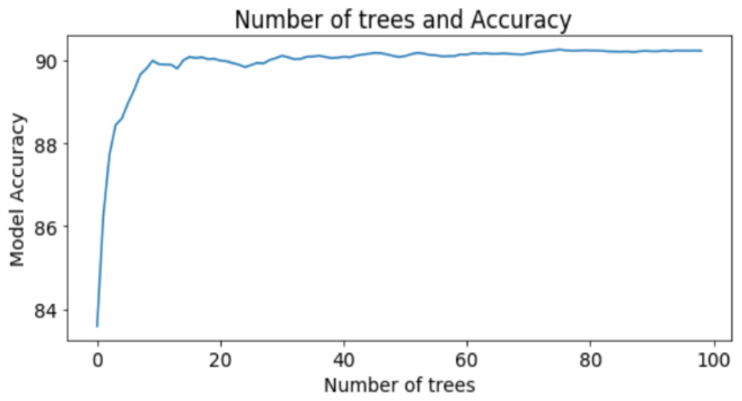
It is evident that the attributes were ordered according to their correlation coefficient. The overall quality of the house and the total ground living area were the most important features of the dataset for predicting the house price. We trained a random forest algorithm with different values of the correlation coefficient. The accuracy on the training set was high with a huge number of features, while the performance on the test set was substantially lower due to the overfitting problem. In order to attain the perfect value of the correlation coefficient, we simulated the dataset in more detail and with greater precision. 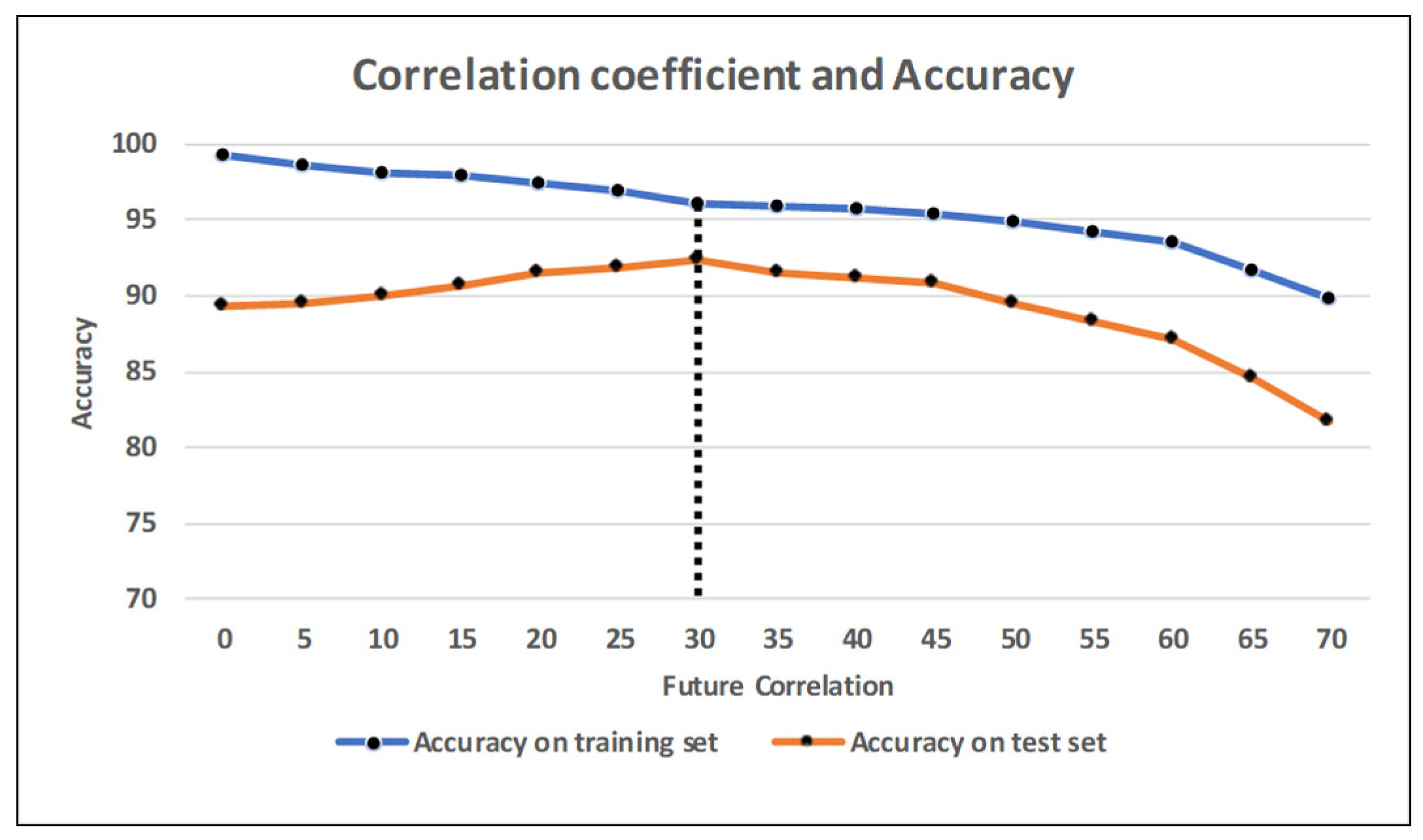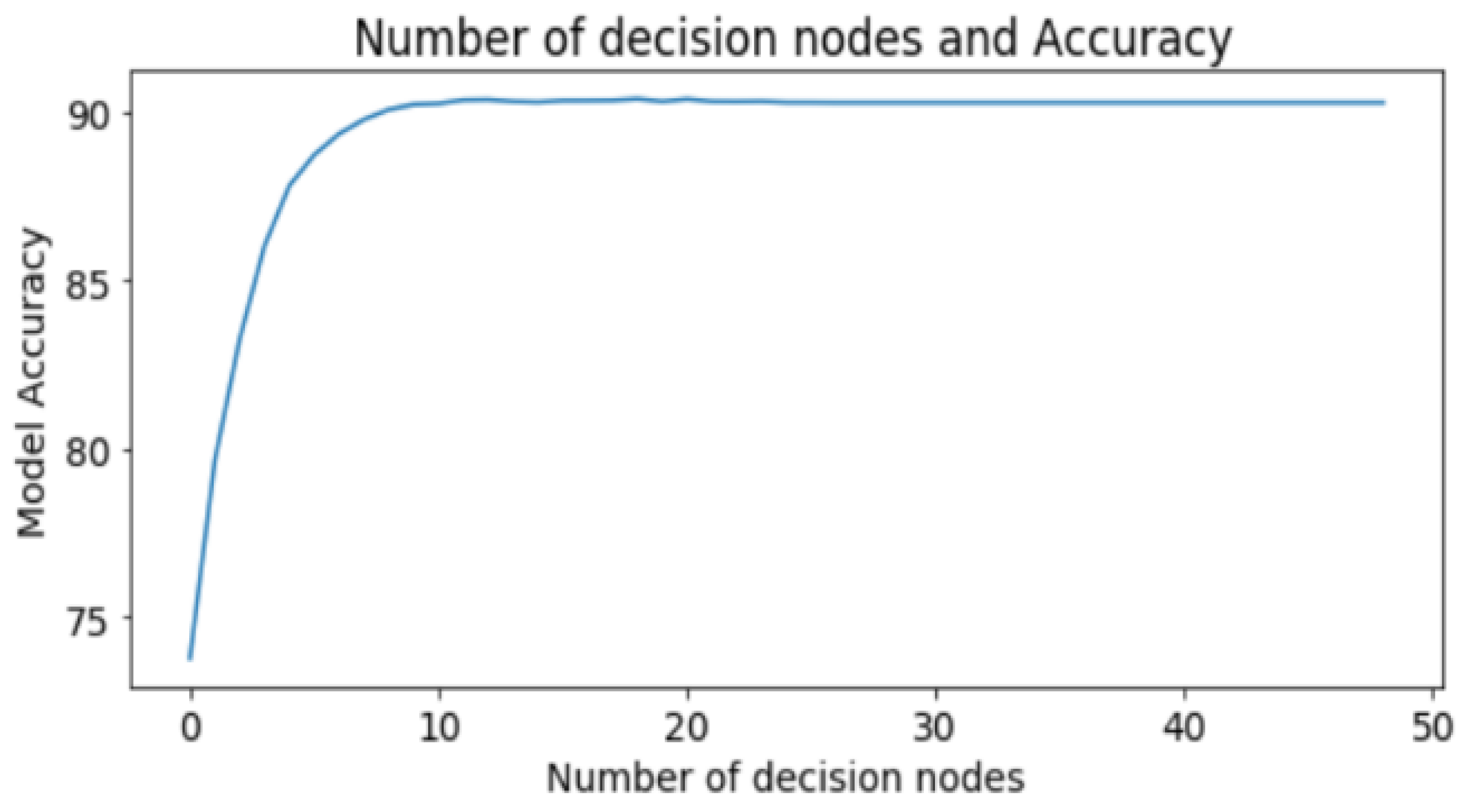Figure 3 shows the significant relationship between the correlation coefficient and the accuracy of the model on both the training and the test subsets. The vertical axis demonstrates the accuracy percentage of the training and the test subsets. The horizontal axis represents the correlation coefficient over the given amount.

To make it clearer, take the first value, 0%, as an example. It denotes that we used all the 256 features while training and testing the model. The accuracy line illustrates the values of around 99% and 89% for the training and the test sets, respectively. The second value, 5%, denotes that we considered the attributes with a correlation coefficient of more than 5%. In this situation, the number of attributes in the training process declined to 180. Practically, the fewer the features for the training set, the lower the accuracy recorded. After training our model with the given number of features, the accuracy for training decreased, while the test set accuracy increased gradually as we tried to prevent our model from overfitting. The main purpose of this graph was to show the best value of the correlation coefficient for obtaining the ideal measure of accuracy.

Figure 3 shows that the best value was 30%. The dataset consisted of 45 features that fit this requirement.

Thus, we improved the accuracy of the model, as the use of few appropriate features is better for training the model than that of a huge amount of irrelevant and unnecessary data. Furthermore, we could prevent overfitting because the possibility of overfitting increases with a growth in the number of unrelated attributes.

3.4. Handling Missing Data

Several concepts to define the distance for KNNs have been described thus far [6,9,10,33,34]. The distance measure can be computed by using the Euclidean distance. Suppose that the jth impute feature of x is absent in

Table 7. Example of missing data in the dataset.

ID	Qual.	No. of Bedrooms	Area	YearBuilt	Gar.Area
0	4	3	120	1992	20
1	6	NaN	135	NaN	25
2	8	2	150	1998	32
3	9	NaN	140	2000	35
4	5	4	120	2002	20
5	7	3	15	1993	35
6	8	4	160	1998	30
7	9	3	140	2005	NaN
8	4	2	120	2008	20
9	3	3	130	2000	27

. After calculating the distance from x to all the training examples, we chose its K closest neighbors from the training subset, as demonstrated in Equation (3).

$${\mathrm{A}}_{\mathrm{x}}={\left\{v_k\right\}}_{k=1}^K$$

(3)

The set in Equation (3) represents the K closest neighbors of x settled in the ascending order of their remoteness. Therefore, v₁ was the nearest neighbor of x. The K closest cases were selected by examining the distance with the non-missing inputs in the incomplete feature to be imputed. After its K nearest neighbors were chosen, the unknown value was imputed by an estimation from the jth feature values of A_x. The imputed value $\widetilde{x_j}$ was acquired by using the mean value of its K closest neighbors, if the jth feature was a numeric variable. One important change was to weight the impact of each observation based on its distance to x, providing a bigger weight to the closer neighbors (see Equation (4)).

$$\widetilde{x_j}=\frac{1}{KW}{\displaystyle \sum }_{k=1}^K{w}_k{v}_{kj}$$

(4)

The primary shortcoming of this method is that when the KNN impute studies the most alike samples, the algorithm uses the entire dataset. This restriction can be very serious for large databases [35]. The suggested technique implements the KNN–MCF method to find the missing values in large datasets. The key downside of using KNN imputation is that it can be severely degraded with high-dimensional data because there is little difference between the nearest and the farthest neighbors. Instead of using all the attributes, in this study, we used only the most important features selected by using Equations (1) and (2). The feature selection technique is typically used for several purposes in machine learning. First, the accuracy of the model can be improved, as the usage of a number of suitable features is better to train the model than the usage of a large number of unrelated and redundant data. The second and the most significant reason is dealing with the overfitting problem, since the possibility of overfitting is high with a growth of the number of irrelevant features. We used only 45 of the most important features for handling the missing data with our model. By doing so, we achieved the goal of avoiding the drawbacks of the KNN impute algorithm. To verify the proposed model, we applied three of the abovementioned methods of handling missing data, namely mean average, KNN, and KNN–MCF, to several machine learning-based prediction algorithms.

4. Results

We evaluated the performance of our KNN–MCF algorithm by utilizing six different machine learning-based prediction algorithms and compared them with the accuracy of the traditional mean average and KNN impute methods to handle missing data. The missing values in the dataset were filled accordingly with standard mean, KNN impute, and KNN–MCF methods before the training step. Figure 4 illustrates the performance of the machine learning algorithms.

The decision tree algorithm exhibited the lowest accuracy, which was less than 80% for the previous method and 0.8633% for the proposed method. The gradient boosted, extra trees, and random forest algorithms yielded reasonably higher correctness than the linear regression and ElasticNet algorithms, with more than 90% accuracy. The best performance was that of the random forest algorithm with 88.43%, 89.34%, and 92.01% accuracy rates for the mean, KNN impute, and KNN–MCF methods, respectively.

After changing the traditional mean method to the KNN impute algorithm, we observed that the accuracy increased slightly in each machine learning algorithm for prediction. One major consideration in the above-mentioned figures is that each ML algorithm’s performance was affected differently by the alterations in the method for handling the missing data. The increase in accuracy was low in some examples, while it was high in the others. Now, we will compare the implementation of all the machine learning algorithms with respect to the KNN–MCF method. It is evident from Figure 5 that the maximum accuracy was recorded for the random forest algorithm.

Furthermore, the KNN method is more computational expensive comparing with KNN–MCF. The main reason for this difference is the KNN examines the whole dataset while KNN–MCF analyses only selected features when dealing with missing data. We can provide

Table 8. Computational cost between KNN and KNN–MCF methods. (Time is subject to change depending on hardware configuration).

Time	Computational Cost
	KNN	KNN–MCF
Training time	10.2 ms	6.5 ms

to show the difference of computational cost between these two methods.

5. Discussion

Because the maximum accuracy was achieved with the random forest algorithm, we decided to discuss the two main parameters of this algorithm. Those are the number of trees and the number of nodes in each tree. Both are defined by the programmer before the implementation of the random forest. These parameters can differ depending on the type of task and dataset. If we identify the perfect values of these two parameters beforehand, not only can we obtain the highest accuracy, but we will also spend less time in most cases. Figure 6 clearly shows that the number of trees for achieving the ideal test accuracy was 20. According to the results, the performance line fluctuated between 91% and 92% for more than 20 trees.

The number of nodes defines how many nodes we have from the root node to the leaf of each tree in the random forest. Figure 7 reveals that the best value for this parameter was 10 in our case. Therefore, we implemented a random forest with 20 estimators and 10 nodes in each estimator.

When choosing a new house, people always pay attention to certain factors like walkability, school quality, and the wealth of the neighborhood area. From this perspective, the location of the house directly affects the price of the property. The relationship between median house price in the given location and the neighborhood area is shown in Figure 8. Different median values are given in a different color. The graph illustrates that the sale price of the house ranges between $100,000 and $300,000 with respect to the location of the house.

6. Conclusions

We proposed an effective technique to deal with missing data in this paper. The primary idea behind the method is to select the most correlated features and use these features to implement the KNN algorithm. To check the performance of a model using our technique, we compared it with the traditional mean average and KNN impute methods by analyzing the performance of these three methods in several machine learning-based prediction algorithms simultaneously. The results of our approach were higher than those of all the machine learning algorithms. Despite obtaining good accuracy for house price prediction, we believe that various improvements can be made in the future, such as the selection of the most important features can be performed using deep learning.

References

1. Feature Selection for Regression | Kaggle. Available online: https://www.kaggle.com/ohmets/feature-selection-for-regression/data (accessed on 10 June 2019).
2. Buckman, J.; Roy, A.; Raffel, C.; Goodfellow, I. Thermometer Encoding: One Hot Way To Resist Adversarial Examples. In Proceedings of the International Conference on Learning Representations, Vacouver, BC, Canada, 22 February 2018; Volume 19, pp. 92–97. [Google Scholar]
3. Novaković, J.; Strbac, P.; Bulatović, D. Toward optimal feature selection using ranking methods and classification algorithms. Yugosl. J. Oper. Res. 2011, 21, 119–135. [Google Scholar] [CrossRef]
4. Cai, J.; Luo, J.; Wang, S.; Yang, S. Feature selection in machine learning: A new perspective. Neurocomputing 2018. [Google Scholar] [CrossRef]
5. Soley-Bori, M. Dealing with Missing Data: Key Assumptions and Methods for Applied Analysis; Boston University Technical Report; Boston University: Boston, MA, USA, 2013. [Google Scholar]
6. Collins, L.M.; Schafer, J.L.; Kam, C.-M. A comparison of inclusive and restrictive strategies in modern missing data procedures. Psychol. Methods 2001, 6, 330–351. [Google Scholar] [CrossRef] [PubMed]
7. Clarke, P.; Hardy, R. Methods for handling missing data. In Epidemiological Methods in Life Course Research; Oxford University Press Inc.: New York, NY, USA, 2009. [Google Scholar]
8. Duda, R.O.; Hart, P.E.; Stork, D.G. Pattern Classification, 2nd ed.; A Wiley-Interscience Publication: New York, NY, USA, 2001; ISBN 0471056693. [Google Scholar]
9. Little, R.J.A.; Rubin, D.B. Mixed Normal and Non-Normal Data with Missing Values, Ignoring the Missing-Data Mechanism. In Statistical Analysis with Missing Data; A Wiley-Interscience Publication: Hoboken, NJ, USA, 2014; pp. 292–311. [Google Scholar]
10. Cox, D.R.; Hinkley, D.V.; Reid, N.; Rubin, D.B.; Silverman, B.W. Monographs on Statistics and Applied Probability, 1st ed.; A CRC Press Company: Washington, DC, USA, 1995; ISBN 9780412406508. [Google Scholar]
11. Li, L.; Chu, K.H. Prediction of real estate price variation based on economic parameters. In Proceedings of the 2017 IEEE International Conference on Applied System Innovation: Applied System Innovation for Modern Technology, ICASI 2017, Sapporo, Japan, 1 May 2017; pp. 87–90. [Google Scholar]
12. Shinde, N.; Gawande, K. Valuation of House Prices Using Predictive Techniques. Int. J. Adv. Electron. Comput. Sci. 2018, 5, 2393–2835. [Google Scholar]
13. Hilbe, J.M. Data Analysis Using Regression and Multilevel/Hierarchical Models. J. Stat. Softw. 2009, 30, 625. [Google Scholar] [CrossRef] [Green Version]
14. Mockus, A. Missing data in software engineering. In Guide to Advanced Empirical Software Engineering; British Library Cataloguing in Publication Data: London, UK, 2008; pp. 185–200. ISBN 9781848000438. [Google Scholar]
15. De Silva, H.; Perera, A.S. Missing data imputation using Evolutionary k-Nearest neighbor algorithm for gene expression data. In Proceedings of the 16th International Conference on Advances in ICT for Emerging Regions, ICTer 2016-Conference Proceedings; IEEE: Negombo, Sri Lanka, 2017; pp. 141–146. [Google Scholar]
16. Kaiser, J. Algorithm for Missing Values Imputation in Categorical Data with Use of Association Rules. ACEEE Int. J. Recent Trends Eng. Technol. 2011, 6, 1–4. [Google Scholar]
17. Malarvizhi, M.R.; Selvadoss Thanamani, A. K-Nearest Neighbor in Missing Data Imputation. Int. J. Eng. Res. 2012, 5, 5–07. [Google Scholar]
18. García-Laencina, P.J.; Sancho-Gómez, J.L.; Figueiras-Vidal, A.R.; Verleysen, M. K nearest neighbours with mutual information for simultaneous classification and missing data imputation. Neurocomputing 2009, 72, 1483–1493. [Google Scholar] [CrossRef]
19. Kim, T.; Ko, W.; Kim, J. Analysis and impact evaluation of missing data imputation in day-Ahead PV generation forecasting. Appl. Sci. 2019, 9, 204. [Google Scholar] [CrossRef] [Green Version]
20. Mahdianpari, M.; Salehi, B.; Mohammadimanesh, F.; Homayouni, S.; Gill, E. The first wetland inventory map of newfoundland at a spatial resolution of 10 m using sentinel-1 and sentinel-2 data on the Google Earth Engine cloud computing platform. Remote Sens. 2019, 11, 43. [Google Scholar] [CrossRef] [Green Version]
21. Li, K.; Chen, Y.; Li, Y. The Random forest-Based method of fine-resolution population spatialization by using the International Space Station nighttime photography and social sensing data. Remote Sens. 2018, 10, 1–19. [Google Scholar] [CrossRef]
22. Tan, F.E.S.; Jolani, S.; Verbeek, H. Guidelines for multiple imputations in repeated measurements with time-dependent covariates: A case study. J. Clin. Epidemiol. 2018, 102, 107–114. [Google Scholar] [CrossRef] [PubMed]
23. House Prices: Advanced Regression Techniques | Kaggle. Available online: https://www.kaggle.com/c/house-prices-advanced-regression-techniques (accessed on 23 June 2019).
24. Boston Housing | Kaggle. Available online: https://www.kaggle.com/c/boston-housing (accessed on 23 June 2019).
25. Kim, H.; Golub, G.H.; Park, H. Missing value estimation for DNA microarray gene expression data: Local least squares imputation. Bioinformatics 2005, 21, 187–198. [Google Scholar] [CrossRef] [PubMed]
26. Siedlecki, W.; Sklansky, J. On Automatic Feature Selection. Int. J. Pattern Recognit. Artif. Intell. 1988, 2, 197–220. [Google Scholar] [CrossRef]
27. Blum, A.L.; Langley, P. Selection of relevant features and examples in machine learning. Artif. Intell. 1997, 97, 245–271. [Google Scholar] [CrossRef] [Green Version]
28. Dash, M.; Liu, H. Feature Selection for Classification. Intell. Data Anal. 1997, 1, 131–156. [Google Scholar] [CrossRef]
29. Dy, J.G.; Brodley, C.E. Feature Subset Selection and Order Identification for Unsupervised Learning. In the Proceedings of the 17th Int’l Conf. Machine Learning; Morgan Kaufman Publisher Inc.: San Francisco, CA, USA, 2000; pp. 247–254. [Google Scholar]
30. Das, S. Filters, wrappers and a boosting-Based hybrid for feature selection. In Proceedings of the 18th Int’l Conf. Machine Learning, Williams College, Williamstown, MA, USA, 28 June –1 July 2001. [Google Scholar]
31. Kim, Y.; Street, W.N.; Menczer, F. Feature Selection in Unsupervised Learning via Evolutionary Search. In Proceedings of 6th ACM SIGKDD International Conference on Knowledge Discovery and Data Mining; Association for Computing Machinery: New York, NY, USA, 2000; pp. 365–369. [Google Scholar]
32. Mitra, P.; Member, S.; Murthy, C.A.; Pal, S.K. Unsupervised Feature Selection Using Feature Similarity. IEEE Trans. Pattern Anal. Mach. Intell. 2002, 24, 301–312. [Google Scholar] [CrossRef]
33. Hron, K.; Templ, M.; Filzmoser, P. Imputation of missing values for compositional data using classical and robust methods. Comput. Stat. Data Anal. 2010, 54, 3095–3107. [Google Scholar] [CrossRef]
34. Troyanskaya, O.; Cantor, M.; Sherlock, G.; Brown, P.; Hastie, T.; Tibshirani, R.; Botstein, D.; Altman, R.B. Missing value estimation methods for DNA microarrays. Bioinformatics 2001, 17, 520–525. [Google Scholar] [CrossRef] [PubMed] [Green Version]
35. Batista, G.; Monard, M.C. A Study of K-Nearest Neighbour as an Imputation Method. In Proceedings of the HIS’02: 2nd International Conference on Hybrid Intelligent Systems; University of Chile: Santiago, Chile, 2002; pp. 251–260. [Google Scholar]
Figure 1. Optimized K-nearest neighbor (KNN) algorithm: KNN-based most correlated features.
Ijgi 09 00227 g001
Figure 2. Correlation coefficients based on sale price of each house.
Ijgi 09 00227 g002
Figure 3. Correlation coefficient vs. accuracy.
Ijgi 09 00227 g003
Figure 4. Comparison of the accuracy of the mean, KNN impute, and K-nearest neighbor algorithm based on the most correlated features (KNN–MCF) methods for dealing with missing data with that of several machine learning algorithms: (a) decision tree, (b) linear regression, (c) ElasticNet, (d) extra trees, (e) gradient boosted, and (f) random forest.
Ijgi 09 00227 g004aIjgi 09 00227 g004b
Figure 5. Accuracy of all machine learning algorithms with respect to the KNN–MCF method.
Ijgi 09 00227 g005
Figure 6. Number of trees vs. test accuracy of the random forest algorithm.
Ijgi 09 00227 g006
Figure 7. Number of nodes vs. test accuracy of the random forest algorithm.
Ijgi 09 00227 g007
Figure 8. Map based on location: color shows details about median sale price of the house; size shows number of houses recorded in the labeled neighborhood.
Ijgi 09 00227 g008