Efficient Coarse Registration of Pairwise TLS Point Clouds Using Ortho Projected Feature Images

Abstract

The degree of automation and efficiency are among the most important factors that influence the availability of Terrestrial light detection and ranging (LiDAR) Scanning (TLS) registration algorithms. This paper proposes an Ortho Projected Feature Images (OPFI) based 4 Degrees of Freedom (DOF) coarse registration method, which is fully automated and with high efficiency, for TLS point clouds acquired using leveled or inclination compensated LiDAR scanners. The proposed 4DOF registration algorithm decomposes the parameter estimation into two parts: (1) the parameter estimation of horizontal translation vector and azimuth angle; and (2) the parameter estimation of the vertical translation vector. The parameter estimation of the horizontal translation vector and the azimuth angle is achieved by ortho projecting the TLS point clouds into feature images and registering the ortho projected feature images by Scale Invariant Feature Transform (SIFT) key points and descriptors. The vertical translation vector is estimated using the height difference of source points and target points in the overlapping regions after horizontally aligned. Three real TLS datasets captured by the Riegl VZ-400 and the Trimble SX10 and one simulated dataset were used to validate the proposed method. The proposed method was compared with four state-of-the-art 4DOF registration methods. The experimental results showed that: (1) the accuracy of the proposed coarse registration method ranges from 0.02 m to 0.07 m in horizontal and 0.01 m to 0.02 m in elevation, which is at centimeter-level and sufficient for fine registration; and (2) as many as 120 million points can be registered in less than 50 s, which is much faster than the compared methods.

1. Introduction

Light detection and ranging (LiDAR) scanning, including Terrestrial LiDAR Scanning (TLS) [1], Personal LiDAR Scanning (PLS) [2], Mobile LiDAR Scanning (MLS) [3], and Airborne LiDAR Scanning (ALS) [4], can acquire dense point clouds of target scenes directly and efficiently. LiDAR scanning is among the most advanced three-dimensional (3D) spatial data acquisition technologies. Point clouds acquired by LiDAR scanning are used in numerous applications, including 3D modeling of target object in reverse engineering [5], 3D building reconstruction in city modeling [6], slopes and super-elevations estimation in road mapping [7], individual tree mapping in forestry [8], and large-scale Digital Elevation Model (DEM) generation in steep mountainous areas [9].

Registration is a fundamental and frequently encountered problem in point clouds processing [10,11]. Terrestrial LiDAR scanning scans the whole target scene station by station and registration is essential to align point clouds obtained from different stations to a unified frame [12,13,14,15,16,17,18]. In addition, the point clouds obtained by different LiDAR scanning platforms, such as TLS and MLS, are often merged to obtain more complete coverage of the target scenes. In such situations, registration of different platform point clouds is necessary [19,20].

The aim of point cloud registration is to obtain the optimal parameters transforming points in one coordinate system to another. The rigid transformation is 6 Degrees of Freedom (DOF), if without any constraints, and can be expressed using three translation parameters and three rotation angles. The translation vector can be denoted as $\mathit{t}={\left(t_x t_y t_z\right)}^T$ and the rotation vector can be denoted as $\mathit{\theta }={\left(\alpha \beta \gamma \right)}^T$. The registration of large-scale dense point clouds is usually time-consuming. To be more efficient, the coarse-to-fine strategy is usually used in point cloud registration. Approximate transformation parameters are first found through the coarse registration algorithm and serve as an initial value of fine registration. Then, the fine registration algorithm converges to the final optimal solution. The details of coarse-to-fine registration strategy can be found in Cheng et al. [10].

The most famous and widely used fine registration algorithms include Iterative Closest Point (ICP) [21], Least Squares 3-Dimensional (LS3D) matching [22], Normal Distributions Transform (NDT) [23], and their variations [24,25,26]. The ICP algorithm finds the pairs of nearest point in the two sets and iteratively estimate the registration parameters by minimizing the distances between the nearest point pairs. In contrast to point pairs, LS3D algorithms match 3D search surfaces to a 3D template surface and estimate the registration parameter by minimizing the Euclidean distances between the surfaces. The NDT algorithm divides the point clouds into cells or voxels and assigns a normal distribution to each cell or voxel to locally model the probability of measuring a point. The registration parameters are estimated by matching of the probability density.

Since this paper deals with the coarse registration of TLS point clouds, the related works reviewed in the next section will mainly focus on coarse registration algorithms. The most intuitive and oldest way to achieve coarse registration is to use artificial targets in data scanning. Artificial targets, such as spherical balls are installed in the scanning scene, and the targets are scanned by more than one scan station. The corresponding coordinates of targets in multiple scan stations are extracted manually, or fitted automatically in the registration process, and the registration parameters are estimated by the coordinate pairs. Sometimes, the coordinate pairs can also be picked manually with feature points such as corners when artificial targets are unavailable. Due to the installation of artificial targets and the manual picking of feature points, these methods are labor-intensive and inefficient.

In the computer vision community, the “generate and test” methods are used to achieve automatic coarse registration of point clouds. The famous Random Sample Consensus (RANSAC) algorithm [27] randomly selects three points from source points and three from target points to form a pair of correspondences. A candidate transformation is estimated using the correspondences and the remaining points are used to test whether the candidate transformation is good or not. Repeating this process until a given number of times reached. The best transformation is chosen as the final coarse registration. RANSAC algorithms do not need any assumptions to the point clouds to be registered, but this kind of methods are often time-consuming, especially when used for large-scale dense TLS point clouds. To accelerate the RANSAC algorithm and make it more robust, Aiger et al. [28] proposed to extract co-planar 4-points sets from source points and target points first, and the correspondences of 4-points sets are found using the RANSAC algorithm. This algorithm is known as 4-Points Congruent Sets (4PCS) algorithm. To further accelerate the 4PCS algorithm, Theiler et al. [18,29,30] extracted keypoints from raw LiDAR points first, and only the extracted key points were used to estimate coarse registration parameters using the 4PCS algorithm. Ge [14] extracted semantic key points first, and then fed the extracted keypoints to the 4PCS algorithm to coarsely register point clouds. The advantages of these methods are that they have no assumptions about the initial pose, and they are resilient to noise and outliers, but these methods are usually time-consuming and intolerable for the registration of large-scale dense TLS point clouds.

Another coarse registration technique is to use 3D local shape descriptors. Keypoints are first extracted in source and target points and 3D local shape descriptors are extracted for each keypoint. Corresponding pairs are obtained by feature descriptor matching, and then coarse registration parameters are estimated utilizing the matched corresponding feature pairs. Rusu et al. [31] proposed a robust 16-dimensional feature called Persistent Feature Histograms (PFH) to achieve the registration of multi-view point clouds. To further improve efficiency, mathematical expressions of PFH are modified and optimized and a new type of local feature called Fast Point Feature Histograms (FPFH) was proposed [32]. Zai et al. [15] proposed an adaptive covariance descriptor to achieve coarse alignment of TLS point clouds. The descriptor was believed to be invariant to rigid transformation and robust to noise and varying resolutions. Gao et al. [33] proposed to utilize Extended Gaussian Image (EGI) to find point correspondences and thus achieve initial registration of point clouds. Yu and Ju [13] used an intrinsic shape signature keypoints detector and the Signature of Histograms of OrienTations (SHOT) [34] descriptor to find correspondences from point clouds. Then a branch-and-bound algorithm was proposed to robustly estimate registration parameters using point correspondences with incorrect matches. Since extracting keypoints from large-scale point clouds is time-consuming and the 3D local shape descriptors are usually high dimensional, 3D local shape descriptors-based coarse registration methods are usually inefficient.

Besides 3D local shape descriptors, high-level features, such as line features, plane features, and semantic features, are also employed for LiDAR point clouds registration. Yang and Zang [35] proposed to extract crest lines from point clouds to achieve coarse registration. Dold and Brenner [36] extracted 3D planar patches from laser scanning data and registered overlapping point clouds by finding corresponding patches. Yang et al. [17] extracted semantic points from point clouds first and then matched the semantic points using geometric constraints. Finally, registration parameters were estimated using the matched semantic points. Kelbe et al. [37] managed to register forest laser scanning point clouds using tree stems extracted from TLS point clouds.

Besides directly using 3D point clouds, coarse registration can also be achieved by 2D images assisted methods. Yang et al [38] proposed to achieve wide baseline 3D scan alignment by using 2D image features. To make the 2D image features more robust, dominant planar structures were extracted from point clouds and used to normalize the camera viewpoint changes. Barnea and Filin [39] first converted the 3D terrestrial laser point clouds into panoramic range images. Then, key features were extracted and matched by a combinatorial approach. Finally, registration parameters were estimated by the matched key features. Weinmann et al. [40] proposed to extract Scale Invariant Feature Transform (SIFT) features from reflectance images and then back project them to 3D utilizing range images to obtain 3D conjugates. Coarse registration parameters were estimated using the 3D conjugates.

Coarse registration is a key step that greatly affects efficiency in point clouds registration. Although numerous methods were proposed trying to solve this problem, it is still challenging. In most cases of LiDAR scanning, the laser scanner is coarsely leveled and even compensated by built-in inclination sensors in many cases. In such cases, the 3DOF rotations between two scans are constrained to only azimuth and the degrees of freedom in registration is reduced from 6 to 4. Cai et al. [12] used this constraint and proposed to use matched keypoints and a branch-and-bound algorithm to achieve efficient 4DOF registration. Similar to Cai et al. [12], this paper takes full advantage of this constraint, and proposes another efficient and automatic method to deal with the 4DOF coarse registration problem. The proposed efficient and automatic method was achieved by two steps: (1) horizontal translation vector and azimuth angle estimation by matching generated ortho projected feature images; (2) vertical translation estimation, achieved by a height difference estimation of overlapping regions after being horizontally aligned. Compared with existing coarse registration methods, the main contributions of this paper include: (1) a two-steps framework to achieve 4DOF coarse registration was proposed. The 4DOF registration was decomposed into two steps. In the first step, the horizontal translation vector and azimuth angle were estimated. In the second step, the vertical translation was estimated. (2) Horizontal translation vector and azimuth angle estimation based on ortho projected feature images. Instead of using panoramic feature images to achieve registration of TLS point clouds, this paper proposed to use ortho projected feature images to achieve horizontal translation vector and azimuth angle estimation.

The remainder of this paper is organized as follows. The experimental point clouds datasets and the 4DOF coarse registration method are described in Section 2. Experimental results are presented in Section 3. Discussions about the proposed method and the experimental results are presented in Section 4. Finally, Section 5 concludes this paper.

2. Materials and Methods

2.1. Experimental Point Clouds Datasets

The proposed method uses intensity information to generate ortho projected feature images. LiDAR scanners provided by different vendors have their characteristics in intensity value. To test the adaptability of the proposed algorithm to point clouds scanned by different types of LiDAR scanners, three TLS point clouds datasets scanned by two different LiDAR scanners were adopted as experimental datasets. The first one, named “DRIEGL”, includes two stations scanned by a RIEGL VZ-400 TLS scanner in a square in Wuhan University. The RIEGL VZ-400 scanner is coarsely leveled in data acquisition. The horizontal scanning step-width and vertical scanning step-width were both set to 0.015 degrees in data scanning. The used point clouds are exported by RISCAN Pro [41]. Before exportation, the point clouds are automatically leveled by RISCAN Pro using the inclination sensor data. Station 1 in the DRIEGL was used for the target points and station 2 was used for the source points. There are about 88.90 million points in station 1 and 120.03 million points in station 2. Five spherical balls were installed in the scene and scanned by both stations. The point clouds of station 1, station 2, and all points before registration are illustrated in Figure 1a–c, respectively. Figure 1a,b is a top view of the station 1 and station 2 points. The red triangles in Figure 1a,b indicate the places where the scanners were placed in data acquisition. The distance between the two scan stations is about 20 m. It can be seen that there is a rotation between these two station points. In Figure 1c, the station 1 points are colored in red and the station 2 points are colored in blue. It is obvious that these two station points are not in a unified frame and need to be registered.

The second dataset was named “DTRIMBLE-1”. The two stations of DTRIMBLE-1 were scanned by a Trimble SX10 TLS laser scanner (scanning total station). Similar to DRIEGL, the laser scanner was leveled during data acquisition. The scanning step-width of the Trimble SX10 is adjustable. The scanning step-width was set to a value larger than the RIEGL VZ-400 laser scanner, so the point density of the DTRIMBLE-1 was lower than that of the DRIEGL. There were about 5.63 million points in station 1 and 5.56 million points in station 2. Station 1 was used for the target points and station 2 was used for the source points that need to be registered. The source points, target points, and all points before the registration of DTRIMBLE-1 are illustrated in Figure 1d–f, respectively. Similar to Figure 1a,b, the positions where the scanners were located are labeled by a red triangle. It can be seen that the two stations were scanned at almost the same place, but a large rotation angle exists between the two stations. Similar to the DRIEGL, the station 1 points are colored in red and the station 2 points are colored in blue in Figure 1f. Figure 1f indicates that these two station points are not in a unified coordinate frame and need to be registered.

The third dataset was named “DTRIMBLE-2”. The two stations of DTRIMBLE-2 were scanned using the same scanner and scanning parameters as DTRIMBLE-1. In contrast to scanning the two stations at almost the same place as DTRIMBLE-1, the two stations of DTRIMBLE-2 were scanned at two stations with a distance of about 16 meters, as indicated by the red triangles in Figure 1g,h. There are about 5.29 million points in station 1 and 5.61 million points in station 2. Figure 1i illustrates that the two station points of DTRIMBLE-2 are not in a unified coordinate system.

Besides DRIEGL, DTRIMBLE-1, and DTRIMBLE-2, to evaluate the influence of viewpoint changes and occlusion of TLS point clouds on the ortho projected feature image registration, station 1 of DRIEGL is used to simulate a pairwise of TLS point clouds. As illustrated in Figure 2a, the points of station 1 in DRIEGL are partitioned into two parts with overlapping: (1) part 1 in the cyan box; and (2) part 2 in the black box. There are 78.30 million points in part 1 and 83.63 million points in part 2. The points of part 2 are first translated in $x$, $y$, and $z$ by 1.0 m separately. Then the points are rotated around the $z$ axis by 45 degrees. Part 1 points and transformed part 2 points are illustrated in Figure 2b. After transformation, part 2 points are in a coordinate system different from that of part 1. The simulated dataset is named as “DSimRIEGL”.

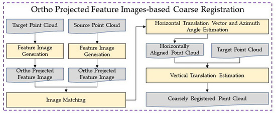
2.2. Ortho Projected Feature Image-Based Coarse Registration Method

The registration of point clouds means to find the optimal transformation parameters between point clouds scanned from different scan stations. If there are two pointsets, denoted as $P$ and $P^{\prime }$, the transformation between these two-point sets can be described as

$$\left[\begin{array}{c}{x}^{\prime }\\ y^{\prime }\\ z^{\prime }\end{array}\right]=\left[\begin{array}{c}{t}_x\\ t_y\\ t_z\end{array}\right]+R\left(\alpha ,\beta ,\gamma \right)\left[\begin{array}{c}x\\ y\\ z\end{array}\right],$$

(1)

where ${\left(x y z\right)}^T$ denotes the coordinates of the point in source point cloud $P$, and ${\left(x^{\prime } y^{\prime } z^{\prime }\right)}^T$ denotes the coordinates of the point in the target point cloud $P^{\prime }$. ${\left(t_x t_y t_z\right)}^T$ and ${\left(\alpha \beta \gamma \right)}^T$ are the registration parameters, translation vector and rotation angle vector respectively, that need to be estimated. $R\left(\alpha \beta \gamma \right)$ is the rotation matrix computed from the rotation vector.

If the scanner is leveled in data acquisition, the rotation between the source point and target point is reduced to around $Z$ axis only. Then the transformation between source point $P$ and target point $P^{\prime }$ can be simplified from Equation (1) to Equation (2). In such a situation, the goal of registration is to estimate translation vector ${\left(t_x t_y t_z\right)}^T$ and azimuth angle $\gamma$.

$$\left[\begin{array}{c}{x}^{\prime }\\ y^{\prime }\\ z^{\prime }\end{array}\right]=\left[\begin{array}{c}{t}_x\\ t_y\\ t_z\end{array}\right]+R\left(\gamma \right)\left[\begin{array}{c}x\\ y\\ z\end{array}\right],$$

(2)

This paper takes full advantage of the fact that in many cases the TLS laser scanner is leveled and/or compensated by inclination sensors in terrestrial LiDAR scanning. Only the translation vector ${\left(t_x t_y t_z\right)}^T$ and azimuth angle $\gamma$ are enough for coarse registration of such point clouds, and thus the degrees of freedom are reduced from 6 to 4. Figure 3 shows the workflow of the proposed 4DOF coarse registration method. To improve coarse registration efficiency, the 4DOF coarse registration is decomposed into two steps: (1) the estimation of horizontal translation vector $\left(t_x,t_y\right)$ and azimuth angle $\gamma$; and (2) the estimation of vertical translation $t_z$. The estimation of the horizontal translation vector and the azimuth angle is achieved by the registration of generated ortho projected feature images, which is described in detail in Section 2.2.1 and Section 2.2.2. The vertical translation is estimated by the height differences of the source points and the target points in overlapping regions after being horizontally aligned, which is described in detail in Section 2.2.3.

2.2.1. Ortho Projected Feature Image Generation

To generate ortho projected feature images of source points and target points, feature image grid resolution $S$ is first determined. Then, the minimum value of $x$, $y$, and $z$ coordinates are found, denoted as $x_{min}$, $y_{min}$, and $z_{min},$ respectively. A point $p\left(x,y,z\right)$ in the point cloud is assigned to image pixel with row number and column number computed by Equation (3) and Equation (4). $INT(.$) means the floor integer value.

$$row=INT(\frac{y-y_{min}}{S}),$$

(3)

$$col=INT(\frac{x-x_{min}}{S}),$$

(4)

More than one point may locate in the same image pixel of the feature image. The pixel value is computed by the average intensity and average height of all points that locate in the same image pixel. Firstly, the average intensity and height of points that locate in the same pixel are computed. Then, the average intensity and average height are scaled to [0, 255], using the maximum and minimum intensity and height values. The intensity information is obtained by Equation (5), where $n$ is the number of points in the same image pixel, $r_i$ is the intensity value of the ith point, $r_{min}$ and $r_{max}$ are the minimum intensity value and the maximum intensity value of the point cloud. The height information is obtained by Equation (6), where $z_i$ is the height/elevation of the ith point. $z_{min}$ and $z_{max}$ are the minimum and maximum elevation of the point cloud. The final pixel value is computed by combining intensity information and height information according to Equation (7), where $\alpha$ is a parameter that determines the relative proportion of intensity information and height information in the final pixel value.

$$v_r=255\ast \frac{\frac{{{\displaystyle \sum }}_{i=1}^n{r}_i}{n}-r_{min}}{r_{max}-r_{min}},$$

(5)

$$v_e=255\ast \frac{\frac{{{\displaystyle \sum }}_{i=1}^n{z}_i}{n}-z_{min}}{z_{max}-z_{min}},$$

(6)

$$v=\alpha \ast v_r+\left(1-\alpha \right)v_e,$$

(7)

2.2.2. Horizontal Translation Vector and Azimuth Angle Estimation

The feature images generated by Section 2.2.1 are ortho projected feature images. The translation vector and azimuth angle to align the ortho projected feature images are the same as the horizontal translation vector and azimuth angle between source points and target points. Thus, the estimation of horizontal translation vector and azimuth angle between source points and target points can be achieved by image registration of ortho projected feature images. In this paper, the SIFT feature proposed by Lowe [42,43] is used to detect distinctive keypoints and extract local feature descriptors from ortho projected feature images generated from source and target points. The SIFT descriptor is invariant to image scale and rotation, and is believed to be robust enough to affine distortion, 3D viewpoint changes, and illumination changes. Since the differences between ortho projected feature images of source and target points mainly include image rotation and 3D viewpoint changes, SIFT is suitable for keypoints detection and local feature descriptor extraction of ortho projected feature images. The details of the SIFT feature can be found in Lowe [42,43].

After SIFT descriptors extracted from feature images, keypoints from source feature image are matched with $k$ nearest keypoints extracted from the target points feature image, using Euclidean distance by approximate nearest neighbor algorithm [44]. The matched $k$ nearest keypoints are ordered by Euclidean distance. In the matched $k$ nearest keypoints, the distance ratio between the nearest distance and the second nearest distance is a good indicator that reflects the match quality. The smaller the distance ratio, the better the match. To only reserve reliable correspondences, match results with distance ratios larger than 0.6 are eliminated.

The image match results are in the image pixel coordinate system. To estimate horizontal translation vector and azimuth angle between source points and target points, the coordinates of image match results in scanner coordinate system are reconstructed by Equations (8) and (9), where $u$ and $v$ are keypoints in image pixel coordinate system,$x_{min}$ and $y_{min}$ are minimum $x$ and $y$ coordinates, $S$ is image grid resolution.

$$x=u\ast S+x_{min},$$

(8)

$$y=v\ast S+y_{min},$$

(9)

The keypoints in source points and target points are denoted as $P_S$ and $P_T$. The horizontal translation vector and azimuth angle are estimated using $P_S$ and $P_T$ by Singular Value Decomposition (SVD) approach [45]. First, the centroids of $P_S$ and $P_T$ are found through Equations (10) and (11), where $N$ is the number of keypoints. Then a matrix $H$, similar to the covariance matrix, is accumulated by Equation (12) and decomposed to $U,S,V$ by SVD algorithm, as described in Equation (13). The rotation matrix from source points to target points can be calculated by $V$ and $U$, using Equation (14). The azimuth angle can be easily computed from the rotation matrix. Finally, the horizontal translation vector can be estimated by Equation (15).

$$centroi{d}_S=\frac{1}{N}{{\displaystyle \sum }}_{i=1}^N{P}_S^i,$$

(10)

$$centroi{d}_T=\frac{1}{N}{{\displaystyle \sum }}_{i=1}^N{P}_T^i,$$

(11)

$$H={{\displaystyle \sum }}_{i=1}^N\left(P_S^i-centroi{d}_S\right){\left(P_T^i-centroi{d}_T\right)}^T,$$

(12)

$$\left[U,S,V\right]=SVD\left(H\right),$$

(13)

$$R=V{U}^T,$$

(14)

$$t=-R\ast centroi{d}_S+centroi{d}_T,$$

(15)

2.2.3. Vertical Translation Estimation

The source points are first transformed using the horizontal translation vector and azimuth angle estimated by the method described in Section 2.2.2 to make the source points horizontally aligned to target points. Since the source and target points have been horizontally aligned, the vertical translation can be estimated by the height differences of the source points and the target points in the overlapping regions. To estimate the height difference in the overlapping regions, a grid is created with the cell size equaling to feature image grid resolution $S$. All the source and target points are assigned to the grid. For a grid cell $\mathrm{C}$ in the overlapping region, the average $z$ value of source points and target points located in the cell $C$ are computed separately, and denoted as $m{z}_C^S$ and $m{z}_C^T$. Thus, the height difference between $m{z}_C^S$ and $m{z}_C^T$, denoted as $d{z}_C$, is computed. The vertical translation between source points and target points is estimated by averaging all $d{z}_C$ in the overlapping regions. Source points are then vertically aligned to target points using the estimated vertical translation.

2.2.4. Accuracy Evaluation Criteria

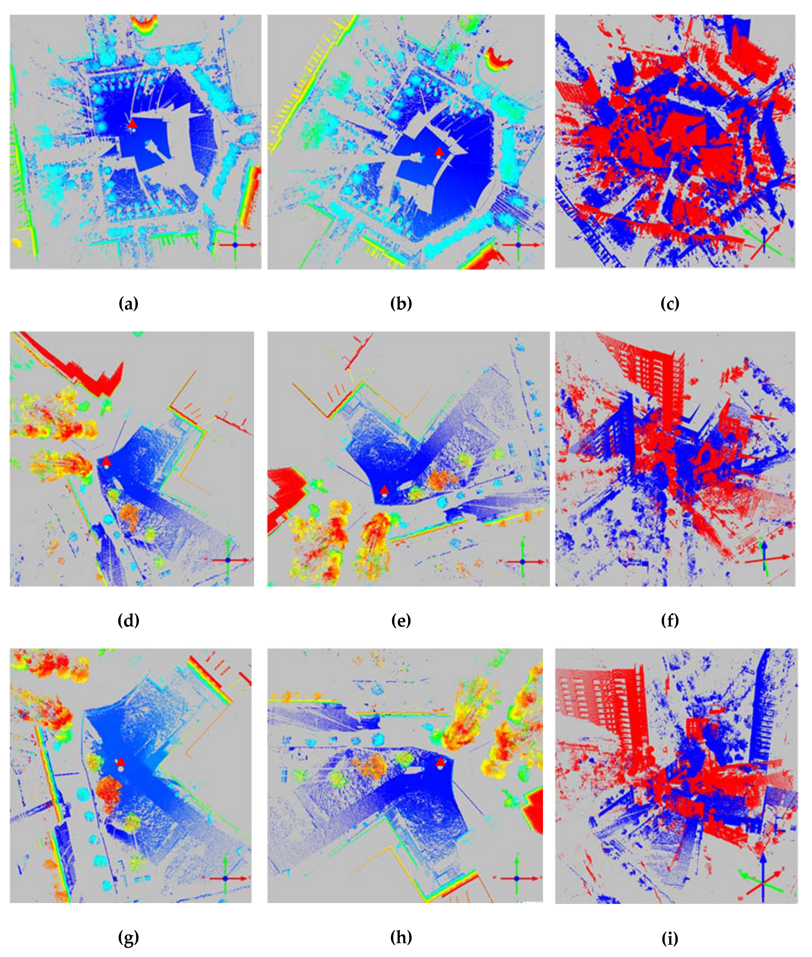
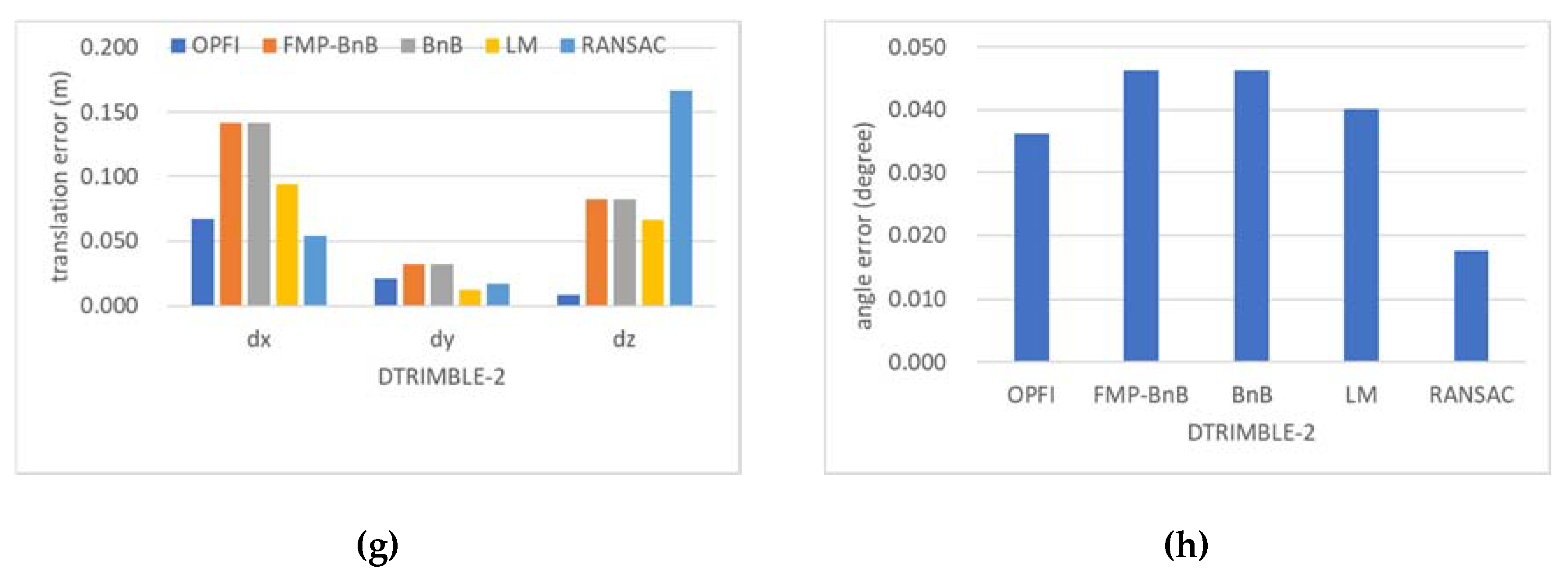
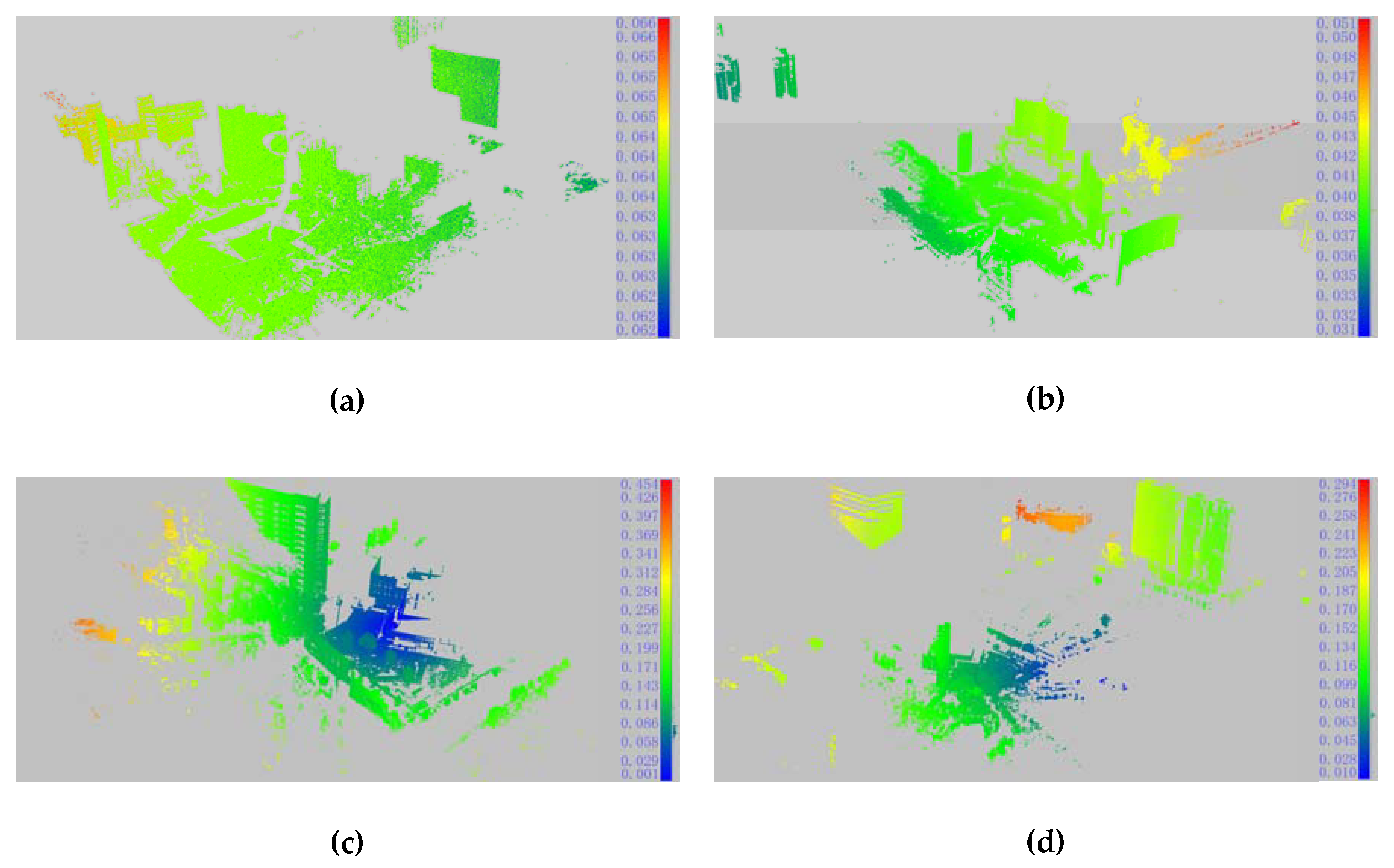
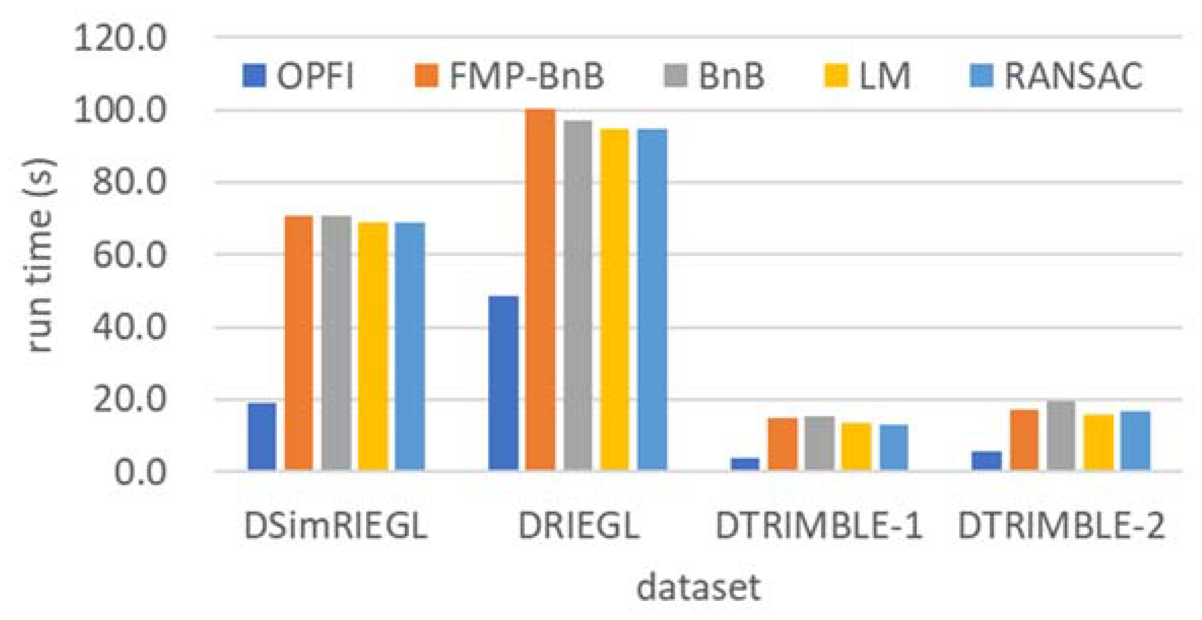
Since the proposed Ortho Projected Feature Images (OPFI) based method registers the source point cloud to the target point in the horizontal and vertical direction separately, this paper evaluates the accuracy of registered source points in the horizontal and vertical direction separately, using ground truth points. The horizontal distance and vertical distance between the ith registered point and its corresponding ground-truth point are calculated and denoted as $d_h^i$ and $d_v^i$. The Horizontal Root Mean Squares Error (HRMSE) and Vertical Root Mean Squares Error (VRMSE) are calculated by Equation (16) and Equation (17). In Equations (16) and (17), $N$ is the number of registered points. Small HRMSE and VRMSE indicate good registration accuracy.

$$HRMSE=\sqrt{\frac{{{\displaystyle \sum }}_{i=1}^N{\left(d_h^i\right)}^2}{N}},$$

(16)

$$VRMSE=\sqrt{\frac{{{\displaystyle \sum }}_{i=1}^N{\left(d_v^i\right)}^2}{N}},$$

(17)

3. Results

The point clouds datasets described in Section 2.1 are used to conduct experiments to verify the proposed method. DSimRIEGL, DRIEGL, DTRIMBLE-1, and DTRIMBLE-2 are all registered by the proposed ortho projected feature image-based method. First, the ortho projected feature images of source points and target points are generated with an image grid resolution of 0.1 meters. In feature image generation, the $\alpha$ value is set to 0.5, to take advantage of both intensity and height information. Besides, to avoid large-scale empty pixels in feature images, points with a scanning distance larger than 100 m are eliminated for DSimRIEGL and DRIEGL. The point cloud obtained by the Trimble SX10 scanner is much sparser than the point clouds obtained by RIEGL VZ-400, and points with a scanning distance larger than 70 m are eliminated for DTRIMBLE-1 and DTRIMBLE-2.

SIFT features are then extracted from the generated ortho projected feature images and matched by $k$ nearest neighbor algorithm. Figure 4 shows the generated ortho feature images and the SIFT matching results. In Figure 4a–d, the left parts are the ortho projected feature images generated from target points, and the right parts are the ortho projected feature images generated from source points. Different objects, such as squares, buildings, and trees, can be clearly distinguished in the feature images. The matched keypoint correspondences are connected by a color line. A total of 1484 correspondences were matched for DSimRIEGL. To illustrate the SIFT matching results more clearly, only SIFT matching results with distance ratio smaller than 0.1 (16 pairs) are drawn in Figure 4a. A total of 65 correspondences, 251 correspondences, and 23 correspondences were matched for DRIEGL, DTRIMBLE-1, and DTRIMBLE-2, respectively. To show the correspondences more clearly, only five representative correspondences were chosen and drawn in Figure 4b–d. The matched correspondences in DRIEGL, DTRIMBLE-1 and DTRIMBLE-2 are much less than that of DSimRIEGL, which indicates that viewpoint changes and occlusion in TLS scanning will affect the SIFT matching result. But the results indicate that enough correct correspondences can be found from ortho projected feature images generated from both simulated and real captured TLS point clouds to accomplish 4DOF registration.

After enough correspondences were found from the ortho projected feature images, the horizontal translation vector and the azimuth angle were estimated using the matched correspondences. Then, the source points were horizontally aligned to the target points using the estimated horizontal translation vector and azimuth angle. The vertical translation was then estimated by the height difference of the source points and target points in overlapping regions after being horizontally aligned. Figure 5 shows the registration results of DSimRIEGL, DRIEGL, DTRIMBLE-1, and DTRIMBLE-2. Figure 5a1,b1,c1,d1 shows the overviews of the registration result of DSimRIEGL, DRIEGL, DTRIMBLE-1, and DTRIMBLE-2, respectively. The target points are colored in red and the source points after registration are colored in green. It can be seen from Figure 5a1,b1,c1,d1 that the registered source points match the target points well, which indicates that the source points are visually well registered to the target points. To identify the registration results more precisely, a small part of the registration results of each dataset (labeled in the black box in Figure 5a1,b1,c1,d1) are zoomed in and shown in Figure 5a2,b2,c2,d2. It can be seen from Figure 5a2,b2,c2,d2 that the walls scanned from target points and source points match each other very well, which indicates that the source points are precisely registered to target points.

To compare the registration result of OPFI with other state-of-the-art methods, the four datasets were also registered by the FMP-BnB method [12], the BnB method [12], the 4DOF version of Lifting Method (LM) [46] and the 4DOF RANSAC method [27]. The C++ codes of these algorithms implemented by Cai et al. [47] were used. The C++ codes can be accessed through the GitHub repository (https://github.com/ZhipengCai/Demo---Practical-optimal-registration-of-terrestrial-LiDAR-scan-pairs). The default parameter values used in the C++ codes were adopted. To evaluate the registration results, the ground truth of registration parameters and registration results are first obtained. For the DSimRIEGL dataset, part 2 points without transformation are used as ground truth. The translation vector is −1.0 m in $x$, $y$, and $z$. The azimuth angle is −45 degrees. The ground truth of DRIEGL is obtained by artificial marker-based coarse registration and the ICP fine registration algorithm. The coordinates of five spherical balls in the scene were obtained by ball fitting in commercial software RISCAN Pro [41] and used to coarsely register station 2 points to station 1 points. The ICP algorithm was then applied to the coarse registration result. The registration parameters were finally computed by the point pairs before and after registration. The ground truth of DTRIMBLE-1 and DTRIMBLE-2 were obtained by manually picked point correspondences-based coarse registration and the ICP fine registration algorithm. Five point correspondences were manually picked from station 2 and station 1 using the open source software CloudCompare [48]. Coarse registration was achieved using the five picked point correspondences. The ICP algorithm was then applied to the coarse registration result. Similar to the DRIEGL dataset, the registration parameters were computed using the point pairs before and after registration.

Figure 6 shows the accuracy of the estimated registration parameters. For the DSimRIEGL dataset, the translation vector accuracies of all algorithms are better than 0.05 m and the azimuth angle accuracies are better than 0.025 degrees. The RANSAC method achieves the best accuracy in translation vector estimation, and the OPFI method achieves the best accuracy in azimuth angle estimation. For the DRIEGL dataset, the OPFI method achieves the best accuracy in horizontal translation vector estimation. The vertical translation accuracy of OPFI is better than the FMP-BnB and BnB methods. The azimuth angle accuracy of OPFI is better than the RANSAC method. For the DTRIMBLE-1 dataset, OPFI achieves the best accuracy in vertical translation and x-direction of horizontal translation. The azimuth angle accuracies of all algorithms are better than 0.16 degrees. For the DTRIMBLE-2 dataset, OPFI achieves much better vertical translation accuracy than the other four algorithms, and achieves better accuracy than FMP-BnB and BnB in x and y-direction. In addition, the OPFI method achieves better azimuth angle accuracy than the other algorithms except for RANSAC.

Table 1. Horizontal Root Mean Squares Error (HRMSE) of the registration results (m).

	OPFI	FMP-BnB	BnB	LM	RANSAC
DSimRIEGL	0.06	0.04	0.04	0.01	0.01
DRIEGL	0.02	0.09	0.09	0.05	0.10
DTRIMBLE-1	0.07	0.02	0.02	0.01	0.06
DTRIMBLE-2	0.07	0.15	0.15	0.13	0.06

and

Table 2. Vertical Root Mean Squares Error (VRMSE) of the registration results (m).

	OPFI	FMP-BnB	BnB	LM	RANSAC
DSimRIEGL	0.01	0.04	0.04	0.01	0.01
DRIEGL	0.02	0.08	0.08	0.01	0.01
DTRIMBLE-1	0.01	0.03	0.03	0.01	0.09
DTRIMBLE-2	0.01	0.08	0.08	0.07	0.17

show the HRMSE and VRMSE of results registered by OPFI and comparison methods. For the DSimRIEGL dataset, the HRMSE of OPFI is 0.06 m and slightly worse than the other four algorithms. The VRMSE of OPFI is the same as the LM and RANSAC methods, and better than that of the FMP-BnB and BnB methods. For the DRIEGL dataset, the HRMSE of OPFI is better than the FMP-BnB, BnB and LM methods and slightly worse than the RANSAC method. The VRMSE of OPFI is better than the FMP-BnB and BnB methods, and slightly worse than the LM and RANSAC methods. For the DTRIMBLE-1 dataset, even though the HRMSE of OPFI is larger than the other four algorithms, it is still better than 0.1 m. The VRMSE of OPFI is the same as that of LM and better than FMP-BnB, BnB, and RANSAC. For the DTRIMBLE-2 dataset, OPFI achieves comparable HRMSE to the RANSAC algorithm, and is better than the other three algorithms. The OPFI achieves the best VRMSE among the five algorithms for the DTRIMBLE-2 dataset. The results in Table 1 and Table 2 indicate that the proposed OPFI method can achieve centimeter registration accuracy, and the accuracy is comparable to other state-of-the-art methods.

Figure 7 shows the registration error of each point in each dataset as a heat map. The 3D Euclidean distance between a point after registration and its corresponding point in the reference data was used as a registration error. The color of each point ranging from blue to red reflects the magnitude of the registration error. It can be seen from Figure 7a–d that most points were registered with good accuracy (blue and green points). Some points (red points in Figure 7a–d) with long scanning distances have a relatively lower registration accuracy compared with those with shorter scanning distances.

The proposed OPFI method and comparison methods are all implemented using C++. All the experiments were conducted on a laptop with an Intel Core i9-8950 HK CPU and 32 Gigabyte memory. The run time of the proposed OPFI method and comparison methods were recorded and are shown in Figure 8. For OPFI, the time of ortho projected feature image generation, the match of ortho projected feature image, the horizontal translation vector and azimuth estimation, the vertical translation vector estimation, and the transformation of the source points are included. For all four datasets, the proposed OPFI method takes the least time, compared with the other four algorithms. The time used by the proposed OPFI method is less than half that of the other four algorithms. This result indicates that the proposed method is more efficient compared with the other four algorithms.

4. Discussion

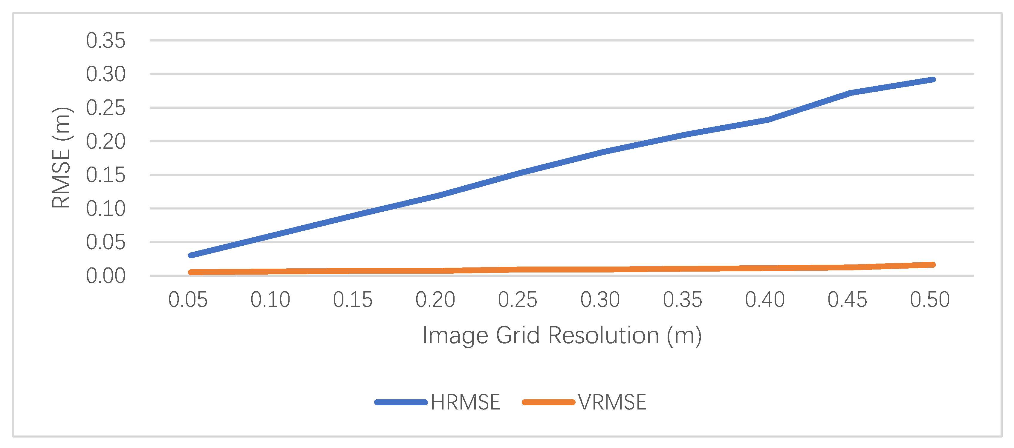
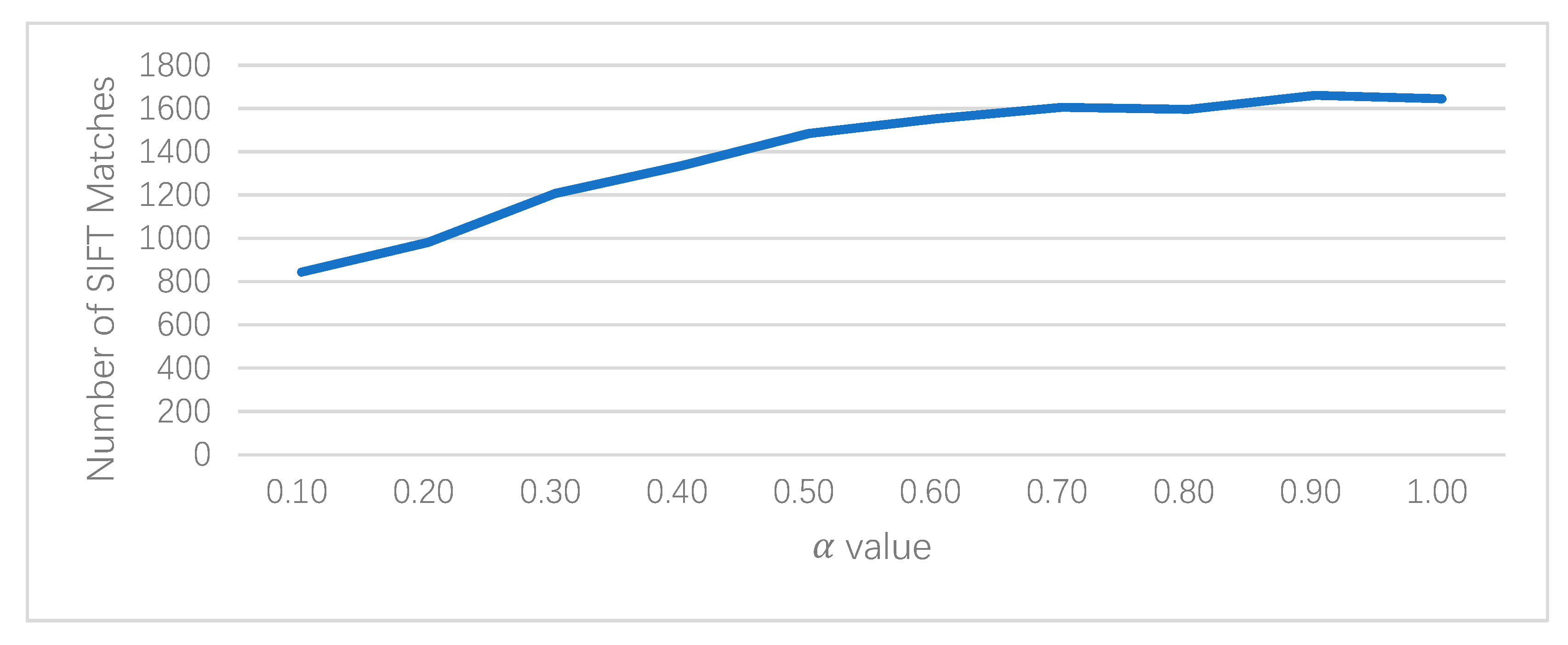
4.1. Parameter Setting

The image grid resolution $S$ of the feature image may affect the estimation accuracy of the horizontal translation vector and azimuth angle. Theoretically, the smaller the image grid resolution, the higher the accuracy. But in reality, the image grid resolution should be set according to the density of the point cloud. Image grid resolution smaller than point cloud density will lead to too many empty pixels in the feature image, and thus affect the registration of feature images. We used the DSimRIEGL dataset and set the image grid resolution from 0.05 m to 0.5 m to exploit the influence of the image grid resolution on coarse registration accuracy. In the experiment, the $\alpha$ value was set to 0.5 in feature image generation. Figure 9 illustrates coarse registration accuracy with different image grid resolution. The horizontal accuracy is more sensitive to image grid resolution and the vertical accuracy is almost not affected by the image grid resolution. Horizontal registration accuracy of about half of the image grid resolution can be achieved by the proposed coarse registration method.

The value of $\alpha$ in feature image generation determines the contribution of intensity and height information to the final feature image, and would thus affect the registration of feature images. Figure 10 illustrates the number of correct matched SIFT correspondences with different $\alpha$ values. Figure 10 shows that intensity contributes well to the SIFT feature image registration. The larger the $\alpha$ value, the more SIFT correspondences can be found. But when $\alpha$ is larger than 0.6, the number of matched SIFT correspondences increases slowly. In order to take full advantage of both intensity and height information, $\alpha$ value is recommended to be set to a value between 0.5 and 0.7.

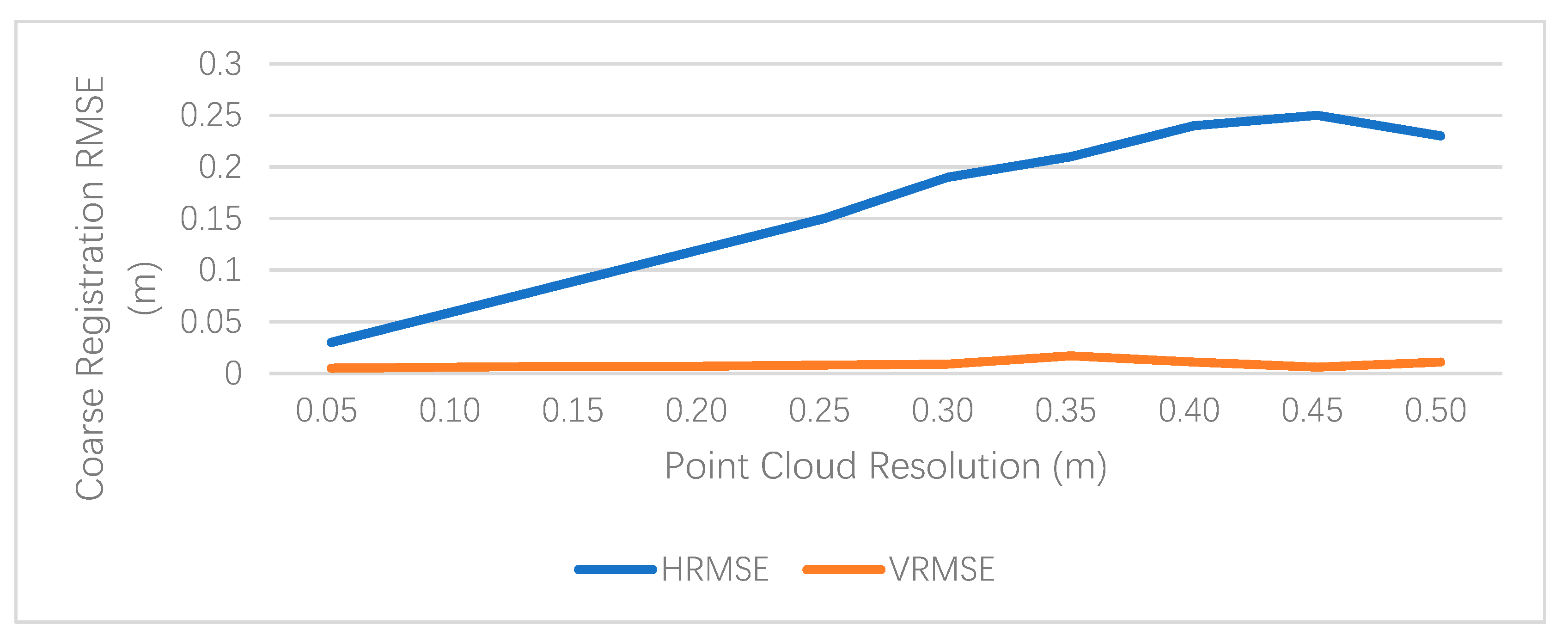
4.2. Registration of Point Clouds with Different Point Density

The density of point clouds varies in different applications. Suitability for point clouds with different density is important for a coarse registration method. Figure 11 illustrates the coarse registration results of point clouds with different point density. The point clouds are intentionally sampled to resolutions from 0.05 m to 0.5 m by a voxel grid sample algorithm. In feature image generation, the value of image grid resolution is set to the same as point resolution. Figure 11 shows that the vertical accuracy is almost not affected by the point resolution. The larger the point cloud resolution, the worse the registration accuracy. The horizontal accuracy is about half of the point resolution.

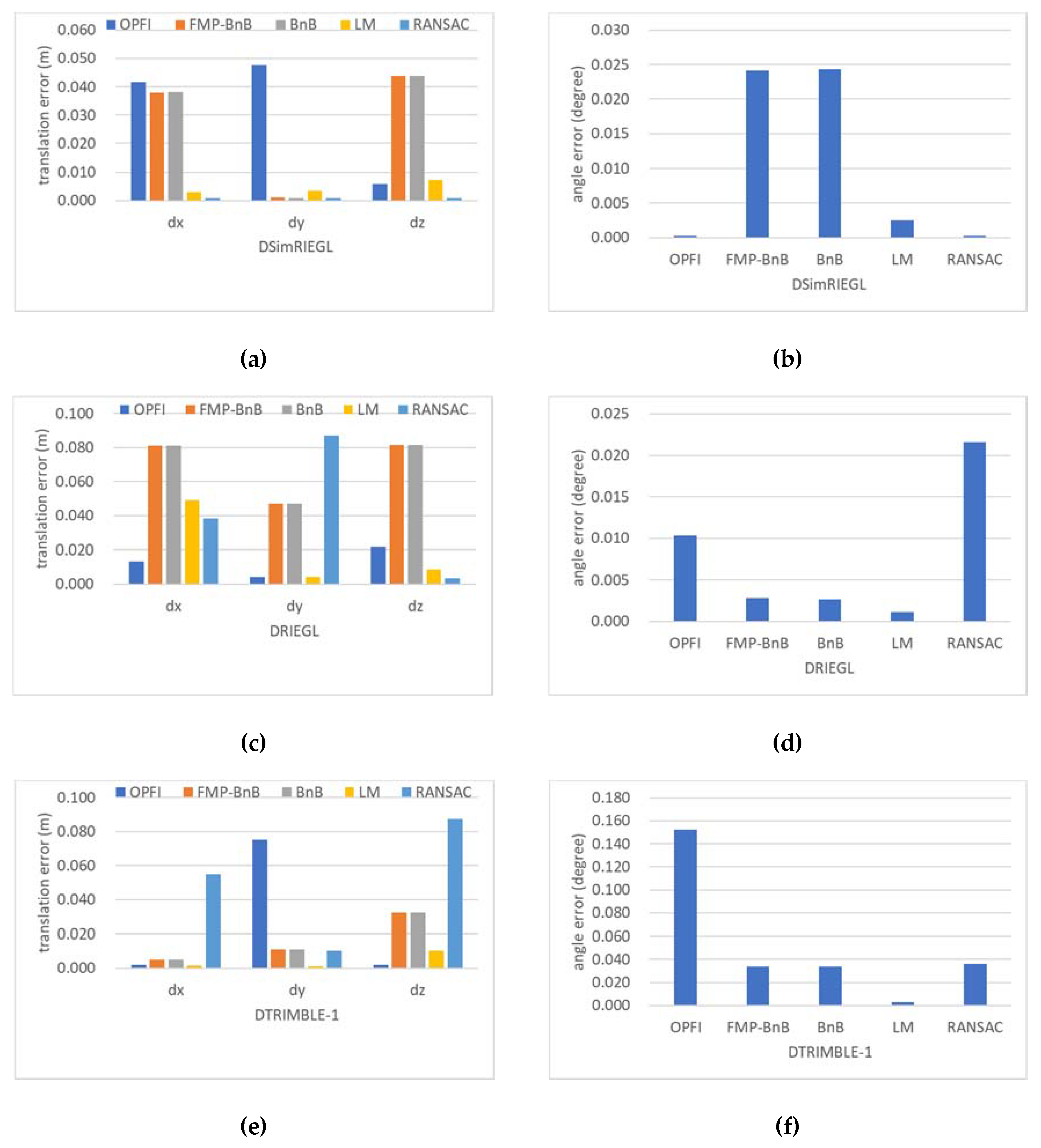
4.3. Accuracy and Efficiency

In the experiments, the proposed coarse registration method accomplished coarse registration of DSimRIEGL, DRIEGL, DTRIMBLE-1 and DTRIMBLE-2. The horizontal accuracy of coarse registration is 0.06, 0.02, 0.07, and 0.07 m for DSimRIEGL, DRIEGL, DTRIMBLE-1 and DTRIMBLE-2, respectively. The vertical accuracy is 0.01, 0.02, 0.01, and 0.01 m, respectively. The registration accuracy is comparable to that of FMP-BnB, BnB, LM, and RANSAC algorithm. The experimental results indicate that centimeter registration accuracy can be achieved by the proposed OPFI method, which is sufficient for coarse registration.

In the experiments, the proposed OPFI method only takes dozens of seconds to achieve coarse registration of millions of TLS points. Compared with the FMP-BnB, BnB, LM, and RANSAC algorithms, the proposed OPFI method takes less than half of the time to register the same datasets. It is far more efficient. The proposed OPFI method provides an alternative to efficient and automatic coarse registration of large-scale dense TLS point clouds.

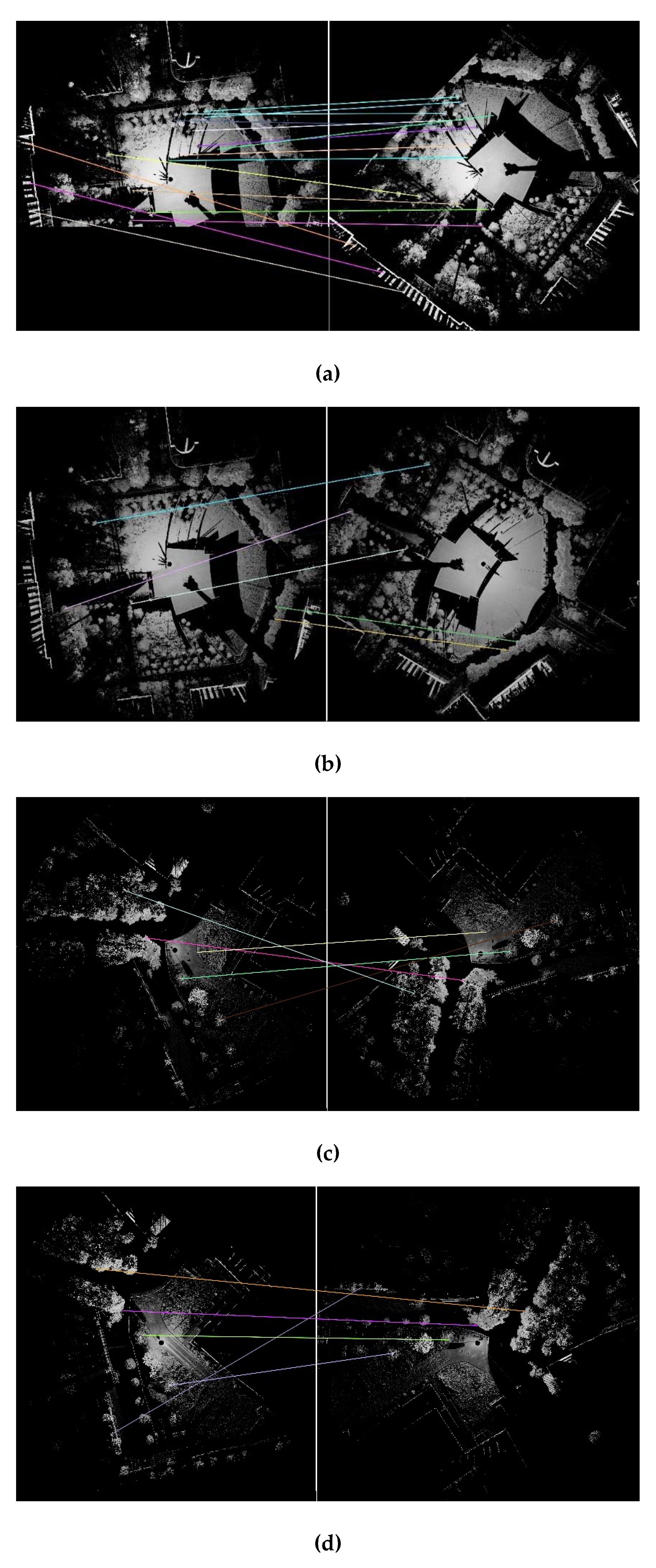
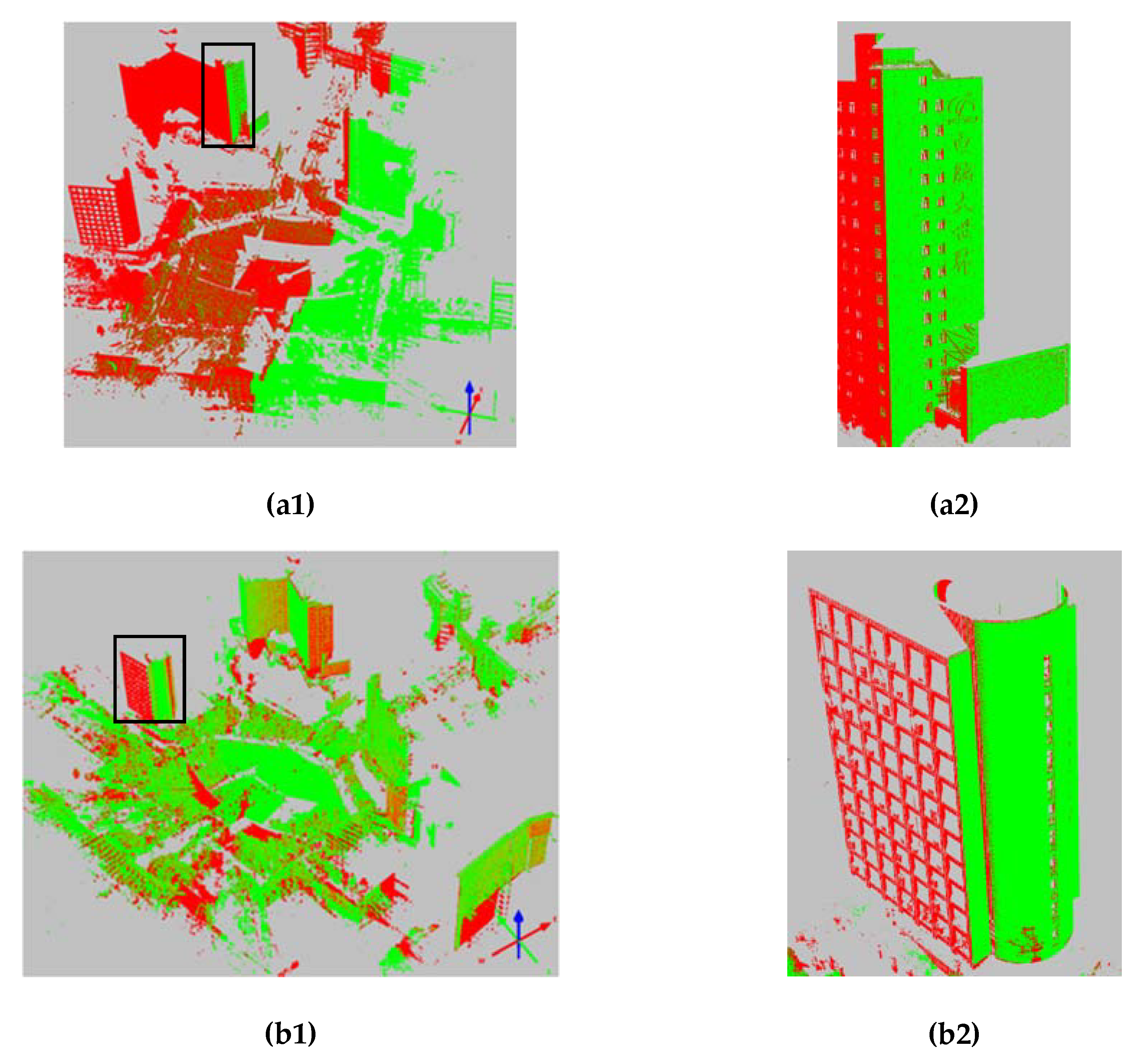
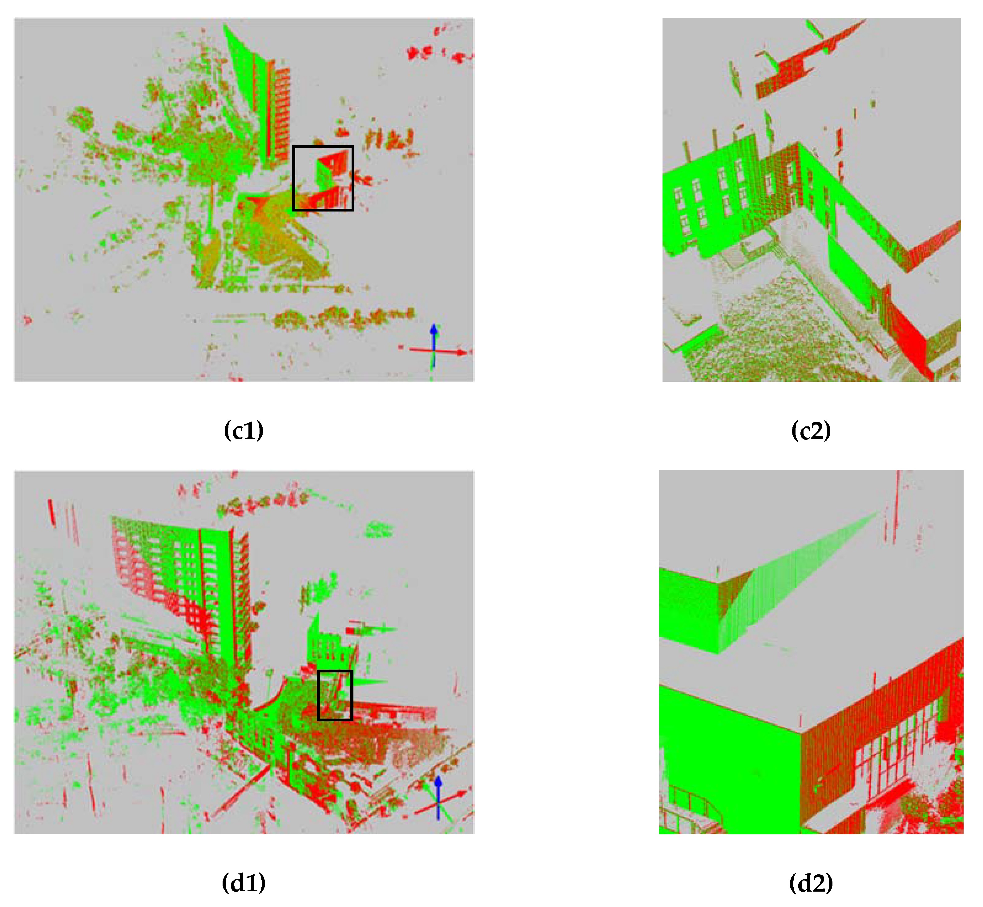
4.4. Robustness of Feature Image Matching

Accurate and robust feature image matching is the key to the proposed OPFI 4DOF coarse registration method. Because of occlusion, different viewpoints, and intensity variation [49] of the TLS point clouds, the matching of feature images is difficult and challenging. The SIFT matching correspondences of DRIEGL, DTRIMBLE-1, and DTRIMBLE-2 are much less than that of DSimRIEGL. This indicates that the SIFT feature matching of ortho feature images is affected by occlusion, different viewpoints, and intensity variation of the TLS point clouds. The SIFT feature matching may fail to find enough correspondences in some cases, especially for point clouds acquired by different laser scanners and different platforms. Lines or edges are more invariant to occlusion, viewpoint changing and intensity variation. Line-based [50,51] or edge-based [52] image matching methods could be applied to improve the robustness of feature image matching.

5. Conclusions

To improve the coarse registration efficiency of large-scale dense TLS point clouds, this paper proposed to reduce the 6DOF registration problem to 4DOF, by fully considering the fact that the laser scanner is usually leveled and compensated by built-in inclination sensors in data acquisition. An efficient and automatic 4DOF coarse registration framework is proposed. In the proposed framework, the horizontal translation vector with the azimuth angle and the vertical translation vector is estimated separately. The horizontal translation vector and azimuth angle are estimated by the registration of ortho projected feature images generated by source and target points. The vertical translation is estimated by the height difference of source points and target points in the overlapping regions after being horizontally aligned. Simulated pairwise TLS point clouds and point clouds scanned by the RIEGL VZ-400 and the Trimble SX10 are used to validate the proposed method. The experimental results demonstrate that the coarse registration result of the proposed method is at centimeter-level, and only dozens of seconds are needed to coarsely register millions of points.

Because of occlusion, different viewpoints, and the fact that the intensity of laser scanning is affected by many factors, the registration of feature images is challenging. In some cases, the SIFT feature matching may fail to find enough correspondences from feature images of the source point cloud and the target point cloud. Large-scale edges and lines can be extracted from the feature images and they are less affected by occlusion, different viewpoints, and intensity variation. Line-based or edge-based matching methods could be applied to the matching of feature images to improve robustness in the future.

References

1. Liang, X.; Kankare, V.; Hyyppä, J.; Wang, Y.; Kukko, A.; Haggrén, H.; Yu, X.; Kaartinen, H.; Jaakkola, A.; Guan, F.; et al. Terrestrial laser scanning in forest inventories. ISPRS J. Photogramm. 2016, 115, 63–77. [Google Scholar] [CrossRef]
2. Liang, X.; Kukko, A.; Kaartinen, H.; Hyyppä, J.; Yu, X.; Jaakkola, A.; Wang, Y. Possibilities of a Personal Laser Scanning System for Forest Mapping and Ecosystem Services. Sensors 2014, 14, 1228–1248. [Google Scholar] [CrossRef] [PubMed]
3. Puente, I.; González-Jorge, H.; Martínez-Sánchez, J.; Arias, P. Review of mobile mapping and surveying technologies. Measurement 2013, 46, 2127–2145. [Google Scholar] [CrossRef]
4. Baltsavias, E.P. Airborne laser scanning: Existing systems and firms and other resources. ISPRS J. Photogramm. 1999, 54, 164–198. [Google Scholar] [CrossRef]
5. Herráez, J.; Martínez, J.C.; Coll, E.; Martín, M.T.; Rodríguez, J. 3D modeling by means of videogrammetry and laser scanners for reverse engineering. Measurement 2016, 87, 216–227. [Google Scholar] [CrossRef]
6. Jarząbek-Rychard, M.; Borkowski, A. 3D building reconstruction from ALS data using unambiguous decomposition into elementary structures. ISPRS J. Photogramm. 2016, 118, 1–12. [Google Scholar] [CrossRef]
7. Wang, J.; Hu, Z.; Chen, Y.; Zhang, Z. Automatic Estimation of Road Slopes and Superelevations Using Point Clouds. Photogramm. Eng. Remote Sens. 2017, 83, 217–223. [Google Scholar] [CrossRef]
8. Yang, B.; Dai, W.; Dong, Z.; Liu, Y. Automatic Forest Mapping at Individual Tree Levels from Terrestrial Laser Scanning Point Clouds with a Hierarchical Minimum Cut Method. Remote Sens. 2016, 8, 372. [Google Scholar] [CrossRef] [Green Version]
9. Chen, Q.; Wang, H.; Zhang, H.; Sun, M.; Liu, X. A Point Cloud Filtering Approach to Generating DTMs for Steep Mountainous Areas and Adjacent Residential Areas. Remote Sens. 2016, 8, 71. [Google Scholar] [CrossRef] [Green Version]
10. Cheng, L.; Chen, S.; Liu, X.; Xu, H.; Wu, Y.; Li, M.; Chen, Y. Registration of Laser Scanning Point Clouds: A Review. Sensors 2018, 18, 1641. [Google Scholar] [CrossRef] [Green Version]
11. Zhu, H.; Guo, B.; Zou, K.; Li, Y.; Yuen, K.; Mihaylova, L.; Leung, H. A Review of Point Set Registration: From Pairwise Registration to Groupwise Registration. Sensors 2019, 19, 1191. [Google Scholar] [CrossRef] [Green Version]
12. Cai, Z.; Chin, T.; Bustos, A.P.; Schindler, K. Practical optimal registration of terrestrial LiDAR scan pairs. ISPRS J. Photogramm. 2019, 147, 118–131. [Google Scholar] [CrossRef] [Green Version]
13. Yu, C.; Ju, D. A Maximum Feasible Subsystem for Globally Optimal 3D Point Cloud Registration. Sensors 2018, 18, 544. [Google Scholar] [CrossRef] [Green Version]
14. Ge, X. Automatic markerless registration of point clouds with semantic-keypoint-based 4-points congruent sets. ISPRS J. Photogramm. 2017, 130, 344–357. [Google Scholar] [CrossRef] [Green Version]
15. Zai, D.; Li, J.; Guo, Y.; Cheng, M.; Huang, P.; Cao, X.; Wang, C. Pairwise registration of TLS point clouds using covariance descriptors and a non-cooperative game. ISPRS J. Photogramm. 2017, 134, 15–29. [Google Scholar] [CrossRef]
16. Kelbe, D.; van Aardt, J.; Romanczyk, P.; van Leeuwen, M.; Cawse-Nicholson, K. Multiview Marker-Free Registration of Forest Terrestrial Laser Scanner Data With Embedded Confidence Metrics. IEEE Trans. Geosci. Remote Sens. 2017, 55, 729–741. [Google Scholar] [CrossRef]
17. Yang, B.; Dong, Z.; Liang, F.; Liu, Y. Automatic registration of large-scale urban scene point clouds based on semantic feature points. ISPRS J. Photogramm. 2016, 113, 43–58. [Google Scholar] [CrossRef]
18. Theiler, P.W.; Wegner, J.D.; Schindler, K. Globally consistent registration of terrestrial laser scans via graph optimization. ISPRS J. Photogramm. 2015, 109, 126–138. [Google Scholar] [CrossRef]
19. Yang, B.; Zang, Y.; Dong, Z.; Huang, R. An automated method to register airborne and terrestrial laser scanning point clouds. ISPRS J. Photogramm. 2015, 109, 62–76. [Google Scholar] [CrossRef]
20. Automatic Registration of TLS-TLS and TLS-MLS Point Clouds Using a Genetic Algorithm. Sensors 2017, 17, 1979. [CrossRef] [PubMed] [Green Version]
21. Besl, P.J.; McKay, N.D. A method for registration of 3-D shapes. IEEE Trans. Pattern Anal. Mach. Intell. 1992, 14, 239–256. [Google Scholar] [CrossRef]
22. Gruen, A.; Akca, D. Least squares 3D surface and curve matching. ISPRS J. Photogramm. 2005, 59, 151–174. [Google Scholar] [CrossRef] [Green Version]
23. Biber, P.; Strasser, W. The normal distributions transform: A new approach to laser scan matching. In Proceedings of the 2003 IEEE/RSJ International Conference on Intelligent Robots and Systems (IROS 2003), Las Vegas, NV, USA, 27–31 October 2003; pp. 2743–2748. [Google Scholar]
24. Park, S.; Subbarao, M. A fast point-to-tangent plane technique for multi-view registration. In Proceedings of the Fourth International Conference on 3-D Digital Imaging and Modeling, Banff, AB, Canada, 6–10 October 2003; pp. 276–283. [Google Scholar]
25. Akca, D. Co-registration of surfaces by 3D least squares matching. Photogramm. Eng. Remote Sens. 2010, 76, 307–318. [Google Scholar] [CrossRef] [Green Version]
26. Magnusson, M.; Lilienthal, A.; Duckett, T. Scan registration for autonomous mining vehicles using 3D-NDT. J. Field Robot. 2007, 24, 803–827. [Google Scholar] [CrossRef] [Green Version]
27. Fischler, M.A.; Bolles, R.C. Random sample consensus: A paradigm for model fitting with applications to image analysis and automated cartography. Commun. ACM 1981, 24, 381–395. [Google Scholar] [CrossRef]
28. Aiger, D.; Mitra, N.J.; Cohen-Or, D. 4-Points Congruent Sets for Robust Pairwise Surface Registration. ACM Trans. Graph. 2008, 27, 1–10. [Google Scholar] [CrossRef] [Green Version]
29. Theiler, P.W.; Wegner, J.D.; Schindler, K. Keypoint-based 4-Points Congruent Sets—Automated marker-less registration of laser scans. ISPRS J. Photogramm. 2014, 96, 149–163. [Google Scholar] [CrossRef]
30. Theiler, P.W.; Wegner, J.D.; Schindler, K. Markerless point cloud registration with keypoint-based 4-points congruent sets. ISPRS Ann. Photogramm. Remote Sens. Spat. Inf. Sci. 2013, 1, 283–288. [Google Scholar] [CrossRef] [Green Version]
31. Rusu, R.B.; Blodow, N.; Marton, Z.C.; Beetz, M. Aligning point cloud views using persistent feature histograms. In Proceedings of the IEEE/RSJ International Conference on Intelligent Robots and Systems, Nice, France, 22–26 September 2008; pp. 3384–3391. [Google Scholar]
32. Rusu, R.B.; Blodow, N.; Beetz, M. Fast point feature histograms (FPFH) for 3D registration. In Proceedings of the IEEE International Conference on Robotics and Automation, Kobe, Japan, 12–17 May 2009; pp. 3212–3217. [Google Scholar]
33. Gao, Y.; Du, Z.; Xu, W.; Li, M.; Dong, W. HEALPix-IA: A Global Registration Algorithm for Initial Alignment. Sensors 2019, 19, 427. [Google Scholar] [CrossRef] [Green Version]
34. Salti, S.; Tombari, F.; Di Stefano, L. SHOT: Unique signatures of histograms for surface and texture description. Comput. Vis. Image Underst. 2014, 125, 251–264. [Google Scholar] [CrossRef]
35. Yang, B.; Zang, Y. Automated registration of dense terrestrial laser-scanning point clouds using curves. ISPRS J. Photogramm. 2014, 95, 109–121. [Google Scholar] [CrossRef]
36. Dold, C.; Brenner, C. Registration of terrestrial laser scanning data using planar patches and image data. ISPRS Arch. 2006, 36, 78–83. [Google Scholar]
37. Kelbe, D.; van Aardt, J.; Romanczyk, P.; van Leeuwen, M.; Cawse-Nicholson, K. Marker-Free Registration of Forest Terrestrial Laser Scanner Data Pairs With Embedded Confidence Metrics. IEEE Trans. Geosci. Remote Sens. 2016, 54, 4314–4330. [Google Scholar] [CrossRef]
38. Yang, M.Y.; Cao, Y.; McDonald, J. Fusion of camera images and laser scans for wide baseline 3D scene alignment in urban environments. ISPRS J. Photogramm. 2011, 66, S52–S61. [Google Scholar] [CrossRef] [Green Version]
39. Barnea, S.; Filin, S. Keypoint based autonomous registration of terrestrial laser point-clouds. ISPRS J. Photogramm. 2008, 63, 19–35. [Google Scholar] [CrossRef]
40. Weinmann, M.; Weinmann, M.; Hinz, S.; Jutzi, B. Fast and automatic image-based registration of TLS data. ISPRS J. Photogramm. 2011, 66, S62–S70. [Google Scholar] [CrossRef]
41. RiScan Pro. Available online: http://www.riegl.com/products/software-packages/riscan-pro/ (accessed on 18 June 2019).
42. Lowe, D.G. Distinctive Image Features from Scale-Invariant Keypoints. Int. J. Comput. Vision 2004, 60, 91–110. [Google Scholar] [CrossRef]
43. Lowe, D.G. Object recognition from local scale-invariant features. In Proceedings of the Seventh IEEE International Conference on Computer Vision ICCV, Kerkyra, Greece, 20–27 September 1999. [Google Scholar]
44. Muja, M.; Lowe, D.G. Fast approximate nearest neighbors with automatic algorithm configuration. In International Conference on Computer Vision Theory and Applications; Springer: Berlin/Heidelberg, Germany, 2009; Volume 2, p. 2. [Google Scholar]
45. Besl, P.J.; McKay, N.D. Method for Registration of 3-D Shapes; International Society for Optics and Photonics: Bellingham, WA, USA, 1992; pp. 586–607. [Google Scholar]
46. Zhou, Q.; Park, J.; Koltun, V. Fast Global Registration; Springer: Berlin/Heidelberg, Germany, 2016; pp. 766–782. [Google Scholar]
47. Demo---Practical-Optimal-Registration-of-Terrestrial-LiDAR-Scan-Pairs. Available online: https://github.com/ZhipengCai/Demo---Practical-optimal-registration-of-terrestrial-LiDAR-scan-pairs (accessed on 18 June 2019).
48. CloudCompare. Available online: http://cloudcompare.org/ (accessed on 18 June 2019).
49. Kashani, A.; Olsen, M.; Parrish, C.; Wilson, N. A Review of LIDAR Radiometric Processing: From Ad Hoc Intensity Correction to Rigorous Radiometric Calibration. Sensors 2015, 15, 28099–28128. [Google Scholar] [CrossRef] [Green Version]
50. Long, T.; Jiao, W.; He, G.; Wang, W. Automatic line segment registration using Gaussian mixture model and expectation-maximization algorithm. IEEE J. Sel. Top. Appl. Earth Obs. Remote Sens. 2014, 7, 1688–1699. [Google Scholar] [CrossRef]
51. Ok, A.O.; Wegner, J.D.; Heipke, C.; Rottensteiner, F.; Soergel, U.; Toprak, V. Matching of straight line segments from aerial stereo images of urban areas. ISPRS J. Photogramm. 2012, 74, 133–152. [Google Scholar] [CrossRef]
52. Wu, B.; Zhang, Y.; Zhu, Q. Integrated point and edge matching on poor textural images constrained by self-adaptive triangulations. ISPRS J. Photogramm. 2012, 68, 40–55. [Google Scholar] [CrossRef]
Figure 1. Point clouds of DRIEGL, DTRIMBLE-1 and DTRIMBLE-2: (a) target points of DRIEGL; (b) source points of DRIEGL; (c) points before registration of DRIEGL; (d) target points of DTRIMBLE-1; (e) source points of DTRIMBLE-1; (f) points before registration of DTRIMBLE-1; (g) target points of DTRIMBLE-2; (h) source points of DTRIMBLE-2; and (i) points before registration of DTRIMBLE-2. In (c), (f) and (i), source points are colored in blue and target points are colored in red.
Ijgi 09 00255 g001
Figure 2. DSimRIEGL point clouds: (a) partitioning of DRIEGL station 1 points into part 1 and part 2; and (b) part 1 points (red) and transformed part 2 points (blue).
Ijgi 09 00255 g002
Figure 3. The workflow of the proposed 4 Degrees of Freedom (4DOF) coarse registration method.
Ijgi 09 00255 g003
Figure 4. Scale Invariant Feature Transform (SIFT) matching results of ortho projected feature images: (a) result of DSimRIEGL; (b) result of DRIEGL; (c) result of DTRIMBLE-1; and (d) result of DTRIMBLE-2.
Ijgi 09 00255 g004
Figure 5. Coarse registration results. (a1) result of DSimRIEGL; (a2) the zoom in view of the part in the black box in (a1); (b1) result of DRIEGL; (b2) the zoom in view of the part in the black box in (b1); (c1) result of DTRIMBLE-1; (c2) the zoom in view of the part in the black box in (c1); (d1) result of DTRIMBLE-2; and (d2) the zoom in view of the part in the black box in (d1). The registered source points are colored in green and the target points are colored in red.
Ijgi 09 00255 g005aIjgi 09 00255 g005b
Figure 6. Accuracy of estimated registration parameters: (a) translation vector accuracy of DSimRIEGL; (b) azimuth angle accuracy of DSimRIEGL; (c) translation vector accuracy of DRIEGL; (d) azimuth angle accuracy of DRIEGL; (e) translation vector accuracy of DTRIMBLE-1; (f) azimuth angle accuracy of DTRIMBLE-1; (g) translation vector accuracy of DTRIMBLE-2; and (h) azimuth angle accuracy of DTRIMBLE-2.
Ijgi 09 00255 g006aIjgi 09 00255 g006b
Figure 7. The registration error of each point rendered as heat map: (a) DSimRIEGL; (b) DRIEGL; (c), DTRIMBLE-1; and (d) DTRIMBLE-2. The unit of distance in the color scale bar is meter.
Ijgi 09 00255 g007
Figure 8. Run time of registration algorithms.
Ijgi 09 00255 g008
Figure 9. Registration accuracy with different image grid resolution in feature image generation.
Ijgi 09 00255 g009
Figure 10. Matched SIFT correspondences with different α values.
Ijgi 09 00255 g010
Figure 11. Coarse registration result of point cloud with different point resolution.
Ijgi 09 00255 g011