Application of Hybrid Prediction Methods in Spatial Assessment of Inland Excess Water Hazard


 ,
,
Abstract
:
1. Introduction
2. Materials and Methods
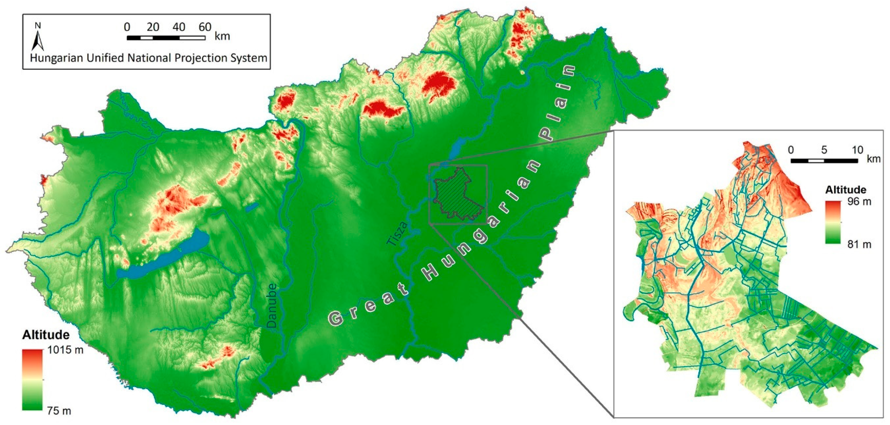
2.1. Study Area
- majority of the area is hazarded due to excess water inundations;
- poor vertical drainage of its soils due to heavy texture (high amount of expanding clay minerals, low permeability, limited infiltration);
- a significant part of the investigated area is traditionally agricultural land used for productive farming, where arable crop production has dominated since the regulation of the rivers of the Great Hungarian Plain;
- there are meteorological data series available in the necessary length and quality;
- the area represented a pilot for the improvement of integrated management practices for public authorities to mitigate heavy rain risks and excess water hazard in the frame of the RAINMAN project (INTERREG CE968: “RAINMAN”).
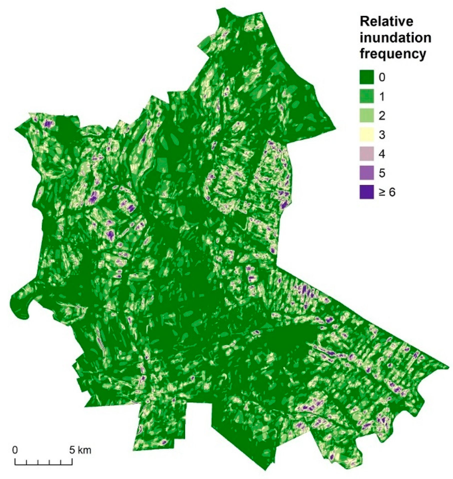
2.2. Reference Data
2.3. Environmental Co-Variables
2.4. Preprocessing of Environmental Co-Variables
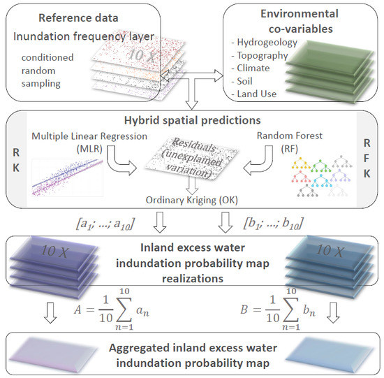
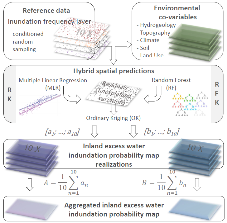
2.5. The Applied Hybrid Prediction Methods
2.5.1. Regression Kriging (RK)
2.5.2. Random Forest Combined with Ordinary Kriging (RFK)
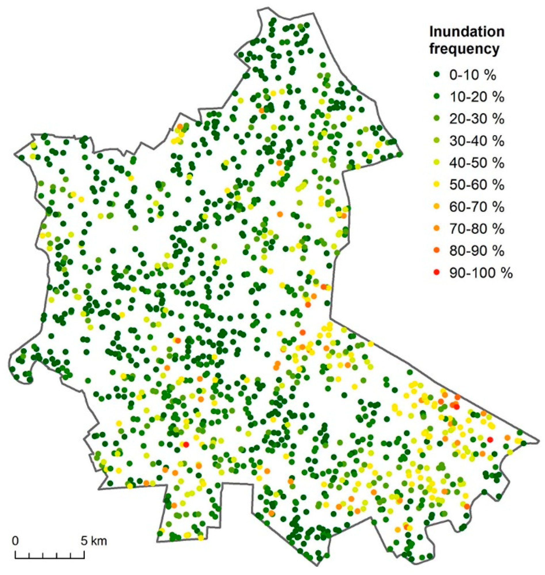
2.6. Validation
2.7. Software Background
3. Results
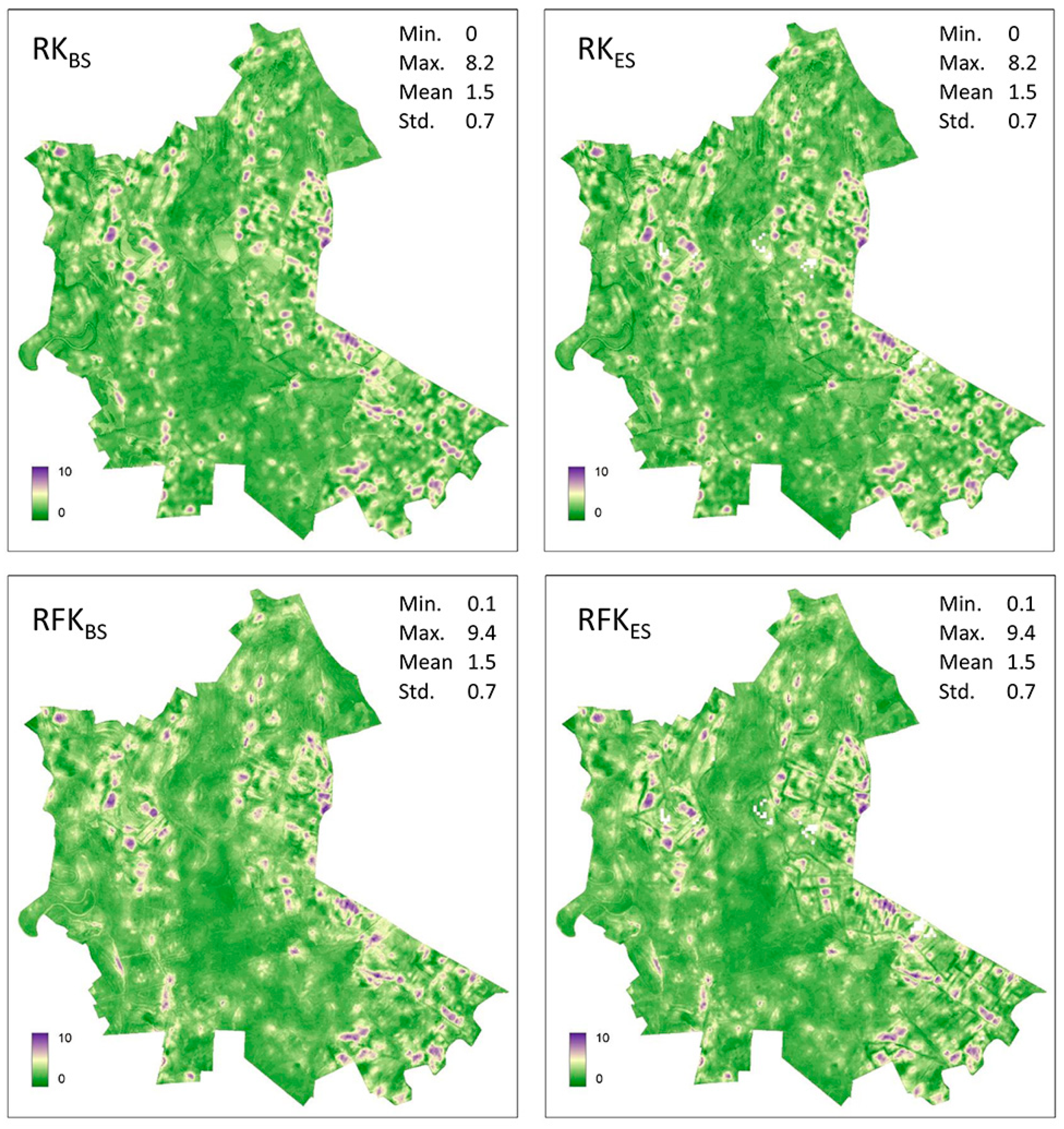
3.1. Result Maps
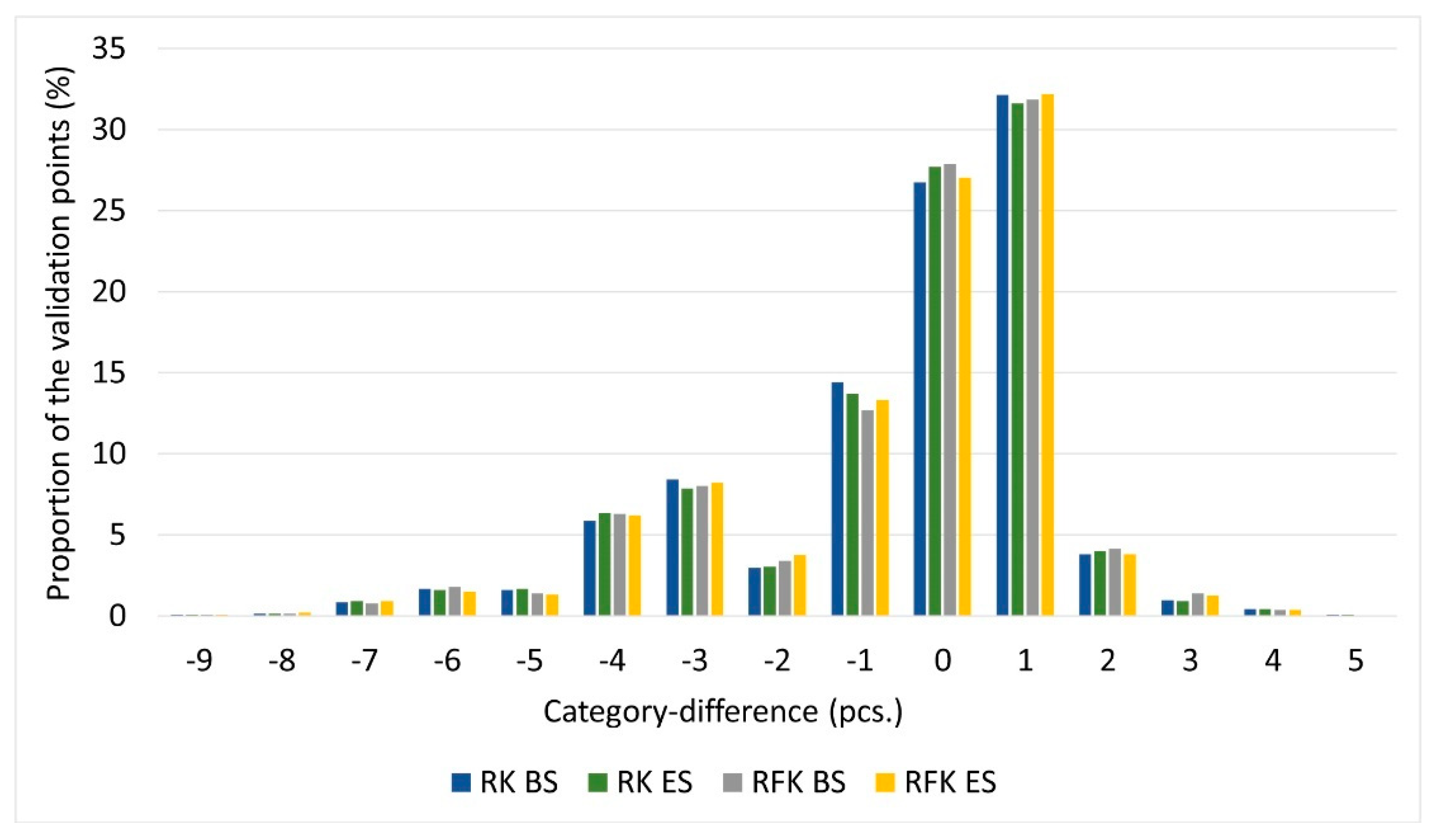
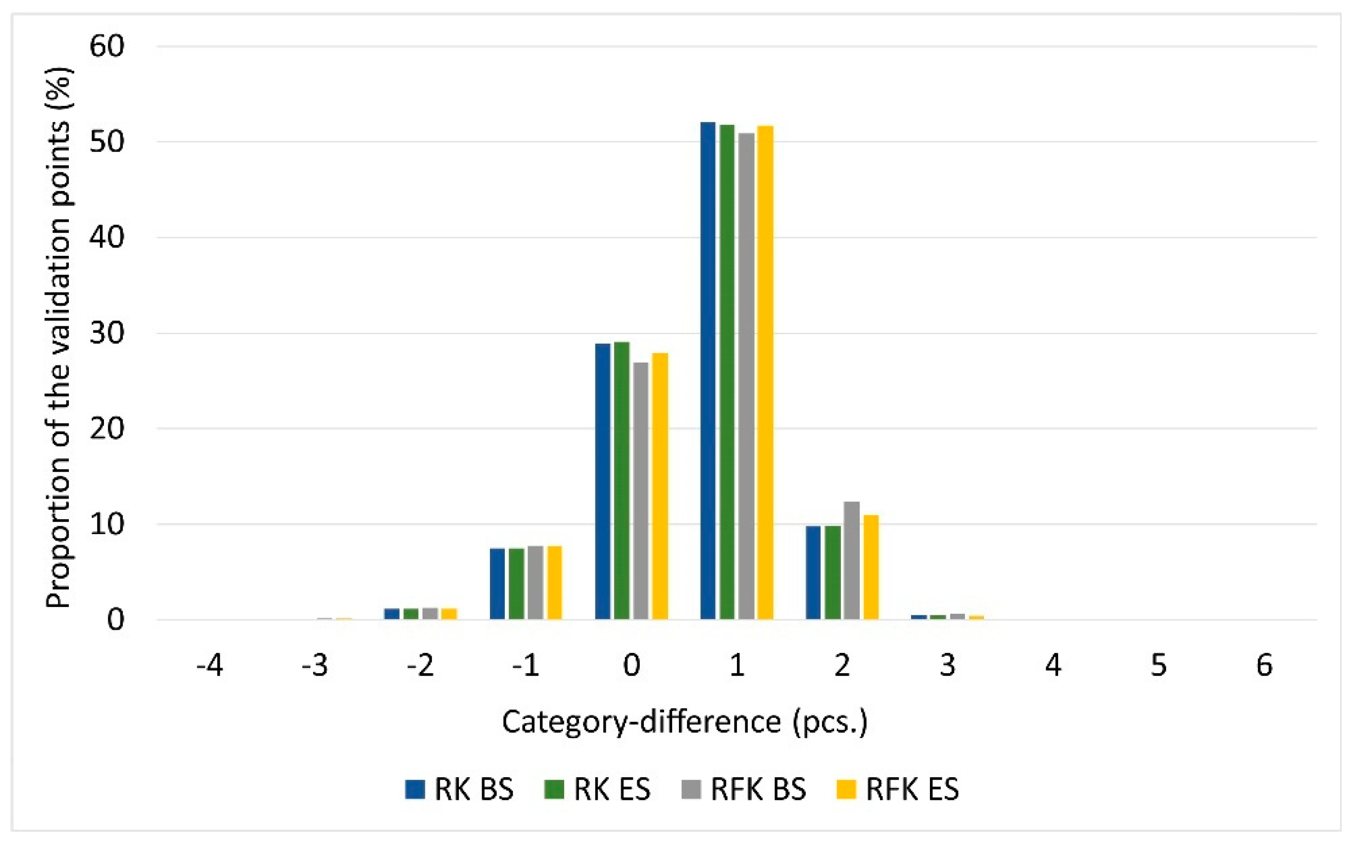
3.2. Validation
4. Discussion
5. Conclusions
Author Contributions
Funding
Acknowledgments
Conflicts of Interest
References
- Bozán, C.; Körösparti, J.; Pásztor, L.; Kuti, L.; Kozák, P.; Pálfai, I. Gis-Based Mapping of Excess Water Inundation Hazard in CsongráD County (Hungary); Analele Universităţii din Oradea; Universităţii din Oradea: Oradea, Romania, 2009; Volume XIV, pp. 678–684. [Google Scholar]
- Pálfai, I. A belvíz definíciói [Definitions of inland excess waters]. Vízügyi Közlemények 2001, 83, 376–392. [Google Scholar]
- Pálfai, I. Az Alföld belvízi veszélyeztetettsége és aszályossága [Map of excess water hazard and drought in the Great Hungarian Plain]. In A víz szerepe és jelentősége az Alföldön; Nagyalföld Alapítvány: Nagyalföld, Hungary, 2000; pp. 85–96. [Google Scholar]
- Szatmári, J.; Van Leeuwen, B. (Eds.) Inland Excess Water–Belvíz–Suvišne Unutrašnje Vode; Szegedi Tudományegyetem–Univerzitet u Novom Sadu: Szeged–Novi Sad, Serbia, 2013; ISBN 978-963-306-263-0. [Google Scholar]
- Merot, P.; Ezzahar, B.; Walter, C.; Aurousseau, P. Mapping waterlogging of soils using digital terrain models. Hydrol. Process. 1995, 9, 27–34. [Google Scholar] [CrossRef] [Green Version]
- Romanescu, G.; Stoleriu, C.; Zaharia, C. Territorial Repartition and Ecological Importance of Wetlands in Moldova (Romania). J. Environ. Sci. Eng. 2011, 5, 1435–1444. [Google Scholar]
- Halbac-Cotoara-Zamfir, R.; Gunal, H.; Birkás, M.; Rusu, T.; Brejea, R. Successful and Unsuccessful Stories in Restoring Despoiled and Degraded Lands in Eastern Europe. Adv. Environ. Biol. 2015, 9, 368–376. [Google Scholar]
- Nađ, I.; Marković, V.; Pavlović, M.; Stankov, U.; Vuksanović, G. Assessing inland excess water risk in Kanjiza (Serbia). Geogr. CGS 2018, 123, 141–158. [Google Scholar] [CrossRef] [Green Version]
- Brkic, M.; Dogan, V.; Obradovic, D.; Zivanov, M. Hardware realization of measurement and monitoring system for level of groundwater. In Proceedings of the IX. Symposium Industrial Electronics INDEL, Banja Luka, Bosnia and Herzegovina, 1–3 November 2012; pp. 124–127. [Google Scholar]
- Awad, S.R.; El Fakharany, Z.M. Mitigation of waterlogging problem in El-Salhiya area, Egypt. Water Sci. 2020, 34, 1–12. [Google Scholar] [CrossRef] [Green Version]
- Setter, T.L.; Waters, I. Review of prospects for germplasm improvement for waterlogging tolerance in wheat, barley and oats. Plant Soil 2003, 253, 1–34. [Google Scholar] [CrossRef]
- Bulti, M.; Abdulatif, A. Review on Agricultural Problems and Their Management in Ethiopia. Turkish J. Agric. Food Sci. Technol. 2019, 7, 1189–1202. [Google Scholar]
- Bergé-Nguyen, M.; Crétaux, J.-F. Inundations in the Inner Niger Delta: Monitoring and Analysis Using MODIS and Global Precipitation Datasets. Remote Sens. 2015, 7, 2127–2151. [Google Scholar] [CrossRef] [Green Version]
- Ojo, O.I.; Ochieng, G.M.; Otieno, F.O.A. Assessment of water logging and salinity problems in South Africa: An overview of Vaal harts irrigation scheme. In WIT Transactions on Ecology and the Environment; WIT Press: Southampton, UK, 2011; pp. 477–484. [Google Scholar]
- Manik, S.M.N.; Pengilley, G.; Dean, G.; Field, B.; Shabala, S.; Zhou, M. Soil and crop management practices to minimize the impact of waterlogging on crop productivity. Front. Plant Sci. 2019, 10, 140. [Google Scholar]
- Yaduvanshi, N.P.S.; Setter, T.L.; Sharma, S.K.; Singh, K.N.; Kulshreshtha, N. Influence of waterlogging on yield of wheat (Triticum aestivum), redox potentials, and concentrations of microelements in different soils in India and Australia. Soil Res. 2012, 50, 489–499. [Google Scholar] [CrossRef]
- Bakker, D.M.; Hamilton, G.J.; Houlbrooke, D.J.; Spann, C.; Burgel, A. Van Productivity of crops grown on raised beds on duplex soils prone to waterlogging in Western Australia. Aust. J. Exp. Agric. 2007, 47, 1368–1376. [Google Scholar] [CrossRef]
- Solaiman, Z.; Colmer, T.D.; Loss, S.P.; Thomson, B.D.; Siddique, K.H.M. Growth responses of cool-season grain legumes to transient waterlogging. Aust. J. Agric. Res. 2007, 58, 406–412. [Google Scholar] [CrossRef]
- Hossain, A.; Uddin, S.N. Mechanisms of waterlogging tolerance in wheat: Morphological and metabolic adaptations under hypoxia or anoxia. Aust. J. Crop Sci. 2011, 5, 1094–1101. [Google Scholar]
- Wu, X.; Tang, Y.; Li, C.; McHugh, A.D.; Li, Z.; Wu, C. Individual and combined effects of soil waterlogging and compaction on physiological characteristics of wheat in southwestern China. Field Crops Res. 2018, 215, 163–172. [Google Scholar] [CrossRef]
- Wang, A.J.; Liu, G. Causes for the Formation of Waterlogged Land in the Black Soil Region of Northeastern China. Adv. Mater. Res. 2012, 610–613, 2925–2930. [Google Scholar] [CrossRef]
- Panigrahi, B.; Chandra Paul, J. Managing Drainage Congestion to Increase Crop Production and Productivity in Hirakud Command, India. J. Agric. Eng. Biotechnol. 2015, 3, 32–40. [Google Scholar] [CrossRef]
- Rout, P.K.; Paul, J.C.; Panigrahi, B. Development of land and water management plan based on geoinformation technique for Puincha watershed, Odisha. J. Soil Water Conserv. 2017, 16, 126–132. [Google Scholar] [CrossRef]
- Boiarskii, B.; Hasegawa, H.; Muratov, A.; Sudeykin, V. Application of UAV-derived digital elevation model in agricultural field to determine waterlogged soil areas in Amur region, Russia. Int. J. Eng. Adv. Technol. 2019, 8, 520–523. [Google Scholar]
- FAO and ITPS. Status of the World’s Soil Resources (SWSR)—Main Report; Food and Agriculture Organization of the United Nations and Intergovernmental Technical Panel on Soils: Rome, Italy, 2015; ISBN 9789251090046. [Google Scholar]
- Linkemer, G.; Board, J.E.; Musgrave, M.E. Waterlogging Effects on Growth and Yield Components in Late-Planted Soybean. Crop Sci. 1998, 38, 1576–1584. [Google Scholar] [CrossRef]
- Barickman, T.C.; Simpson, C.R.; Sams, C.E. Waterlogging Causes Early Modification in the Physiological Performance, Carotenoids, Chlorophylls, Proline, and Soluble Sugars of Cucumber Plants. Plants 2019, 8, 160. [Google Scholar] [CrossRef] [Green Version]
- Morales-Olmedo, M.; Ortiz, M.; Sellés, G. Effects of transient soil waterlogging and its importance for rootstock selection. Chil. J. Agric. Res. 2015, 75, 45–56. [Google Scholar] [CrossRef] [Green Version]
- de San Celedonio, R.P.; Abeledo, L.G.; Miralles, D.J. Physiological traits associated with reductions in grain number in wheat and barley under waterlogging. Plant Soil 2018, 429, 469–481. [Google Scholar] [CrossRef]
- Várallyay, G. Láng István, Csete László és Jolánkai Márton (szerk.): A globális klímaváltozás: Hazai hatások és válaszok (A VAHAVA Jelentés) [The global climate change: Effects and answers in Hungary (The VAHAHA report)]. Agrokémia és Talajt 2007, 56, 199–202. [Google Scholar] [CrossRef] [Green Version]
- Somlyódy, L.; Nováky, B.; Simonffy, Z. Éghajlatváltozás, szélsőségek és vízgazdálkodás [Climate change, extremities, water management]. In “Klíma-21” Füzetek Klímaváltozás—Hatások—Válaszok; Csete, L., Ed.; MTA KSZI Klímavédelmi Kutatások Koordinációs Iroda: Budapest, Hungary, 2010; pp. 15–32. [Google Scholar]
- Pálfai, I. Magyarország belvíz-veszélyeztetettségi térképe [Map of excess water inundation-prone areas of Hungary]. Vízügyi Közlemények 2003, 85, 510–524. [Google Scholar]
- Pálfai, I. A belvizek hidrológiai jellemzése [Hydrology of undrained runoff in Hungary]. Hidrológiai Közlöny 1988, 68, 320–329. [Google Scholar]
- Rakonczai, J.; Csató, S.; Mucsi, L.; Kovács, F.; Szatmári, J. Az 1999. és 2000. évi alföldi belvíz-elöntések kiértékelésének gyakorlati tapasztalatai [Practical experiences with identification of inland excess water in the year 1999 and 2000]. Vízügyi Közlemények 2003, 85, 317–336. [Google Scholar]
- Körösparti, J.; Bozán, C.; Andrási, G.; Túri, N.; Takács, K.; Laborczi, A.; Pásztor, L. Geostatisztikai módszerek alkalmazása a belvíz-veszélyeztetettségi térképezésben [Inland excess water risk mapping by geostatistical methods]. In Proceedings of the MHT XXXIV. Országos Vándorgyűlés, Debrecen, Hungary, 6–8 July 2016; MHT: Debrecen, Hungary, 2016. [Google Scholar]
- Csekő, Á. Árvíz- és belvízfelmérés radar felvételekkel [Flood and excess water monitoring with radar images]. Geodézia és Kartográfia 2002, 55, 16–22. [Google Scholar]
- Csornai, G.; Lelkes, M.; Nádor, G.; Wirnhardt, C. Operatív árvíz- és belvíz-monitoring távérzékeléssel [Operative flood and excess water monitoring based on remote sensing]. Geodézia és Kartográfia 2000, 50, 6–12. [Google Scholar]
- Rakonczai, J.; Mucsi, L.; Szatmári, J.; Kovács, F.; Csató, S. A belvizes területek elhatárolásának módszertani lehetőségei [Opportunities for inland excess water mapping]. In Proceedings of the A Magyar Földrajzi Konferencia Tudományos Közleményei, Szeged, Hungary, 25–27 Ocotber 2001; p. 14. [Google Scholar]
- Licskó, B. A belvizek légi felmérésének tapasztalatai [Experiences of airborne scanning of excess water inundations]. In Proceedings of the MHT XXVII. Országos Vándorgyűlés; Magyar Hidrológiai Társaság, Baja, Mexico, 1–3 July 2009. [Google Scholar]
- Szatmári, J.; Szijj, N.; Mucsi, L.; Tobak, Z.; Van Leeuwen, B.; Lévai, C. A belvízelöntések térképezését és a belvízképződés modellezését megalapozó térbeli adatgyűjtés [Mapping of excess water inundations and modeling of excess water formation with spatial database]. In Proceedings of the Az Elmélet éS Gyakorlat Találkozása a Térinformatikában II; Lóki, J., Ed.; Debrecen University Press: Debrecen, Hungary, 2011; pp. 27–35. [Google Scholar]
- Szatmári, J.; Tobak, Z.; Van Leeuwen, B.; Dolleschall, J. A belvízelöntések térképezését megalapozó adatgyűjtés és a belvízképződés modellezése neurális hálózattal [Data acquisition for inland excess water mapping and modelling using artificial neural networks]. Földrajzi Közlemények 2011, 135, 351–363. [Google Scholar]
- Mucsi, L.; Henits, L. Creating excess water inundation maps by sub-pixel classification of medium resolution satellite images. J. Environ. Geogr. 2010, 3, 31–40. [Google Scholar]
- Csendes, B.; Mucsi, L. Inland excess water mapping using hyperspectral imagery. Geogr. Pannonica 2016, 20, 191–196. [Google Scholar] [CrossRef] [Green Version]
- Van Leeuwen, B. Identification of inland excess water floodings using an artificial neural network. Carpathian J. Earth Environ. Sci. 2012, 7, 173–180. [Google Scholar]
- Van Leeuwen, B.; Tobak, Z.; Kovács, F.; Sipos, G. Towards a continuous inland excess water flood monitoring system based on remote sensing data. J. Environ. Geogr. 2017, 10, 9–15. [Google Scholar] [CrossRef] [Green Version]
- Mezősi, G.; Bata, T.; Meyer, B.C.; Blanka, V.; Ladányi, Z. Climate Change Impacts on Environmental Hazards on the Great Hungarian Plain, Carpathian Basin. Int. J. Disaster Risk Sci. 2014, 5, 136–146. [Google Scholar] [CrossRef] [Green Version]
- Barta, K. Inland excess water projections based on meteorological and pedological monitoring data on a study area located in the Southern part of the Great Hungarian Plain. J. Environ. Geogr. 2013, 6, 31–37. [Google Scholar] [CrossRef] [Green Version]
- Hengl, T.; Sierdsema, H.; Radović, A.; Dilo, A. Spatial prediction of species’ distributions from occurrence-only records: Combining point pattern analysis, ENFA and regression-kriging. Ecol. Model. 2009, 220, 3499–3511. [Google Scholar] [CrossRef] [Green Version]
- Hatvani, I.G.; Leuenberger, M.; Kohán, B.; Kern, Z. Geostatistical analysis and isoscape of ice core derived water stable isotope records in an Antarctic macro region. Polar Sci. 2017, 13, 23–32. [Google Scholar] [CrossRef]
- Fehér, Z.Z.; Rakonczai, J. Analysing the sensitivity of Hungarian landscapes based on climate change induced shallow groundwater fluctuation. Hungarian Geogr. Bull. 2019, 68, 355–372. [Google Scholar] [CrossRef]
- Koch, J.; Stisen, S.; Refsgaard, J.C.; Ernstsen, V.; Jakobsen, P.R.; Højberg, A.L. Modeling depth of the redox interface at high resolution at national scale using random forest and residual gaussian simulation. Water Resour. Res. 2019, 55, 1451–1469. [Google Scholar] [CrossRef]
- Koch, J.; Berger, H.; Henriksen, H.J.; Sonnenborg, T.O. Modelling of the shallow water table at high spatial resolution using random forests. Hydrol. Earth Syst. Sci. 2019, 23, 4603–4619. [Google Scholar]
- Szabó, B.; Szatmári, G.; Takács, K.; Laborczi, A.; Makó, A.; Rajkai, K.; Pásztor, L. Mapping soil hydraulic properties using random-forest-based pedotransfer functions and geostatistics. Hydrol. Earth Syst. Sci. 2019, 23, 2615–2635. [Google Scholar]
- Pásztor, L.; Körösparti, J.; Bozán, C.; Laborczi, A.; Takács, K. Spatial risk assessment of hydrological extremities: Inland excess water hazard, Szabolcs-Szatmár-Bereg County, Hungary. J. Maps 2015, 11, 636–644. [Google Scholar]
- Bozán, C.; Takács, K.; Körösparti, J.; Laborczi, A.; Túri, N.; Pásztor, L. Integrated spatial assessment of inland excess water hazard on the Great Hungarian Plain. Land Degrad. Dev. 2018, 29, 4373–4386. [Google Scholar]
- IUSS Working Group WRB. World Reference Base for Soil Resources 2014, Update 2015. International Soil Classification System for Naming Soils and Creating Legends for Soil Maps; FAO: Rome, Italy, 2015; ISBN 978-92-5-108369-7. [Google Scholar]
- Pásztor, L.; Szabó, J.; Bakacsi, Z.; Matus, J.; Laborczi, A. Compilation of 1:50,000 scale digital soil maps for Hungary based on the digital Kreybig soil information system. J. Maps 2012, 8, 215–219. [Google Scholar]
- Kreybig, L. Magyar Királyi Földtani Intézet talajfelvételi, vizsgálati és térképezési módszere (The survey, analytical and mapping method of the Hungarian Royal Institute of Geology). Magy. Királyi Földtani Intézet Évkönyve 1937, 31, 147–244. [Google Scholar]
- Pásztor, L.; Laborczi, A.; Takács, K.; Szatmári, G.; Bakacsi, Z.; Szabó, J. Variations for the Implementation of SCORPAN’s “S”. In Digital Soil Mapping Across Paradigms, Scales and Boundaries; Zhang, G.-L., Brus, D.J., Liu, F., Song, X.-D., Lagacherie, P., Eds.; Springer Science+Business Media: Singapore, 2016; pp. 331–342. ISBN 978-981-10-0414-8. [Google Scholar]
- Tóth, B.; Weynants, M.; Pásztor, L.; Hengl, T. 3D soil hydraulic database of Europe at 250 m resolution. Hydrol. Process. 2017, 31, 2662–2666. [Google Scholar]
- Szentimrey, T.; Bihari, Z. Mathematical background of the spatial interpolation methods and the software MISH (Meteorological Interpolation based on Surface Homogenized Data Basis). In Proceedings of the Conference on Spatial Interpolation in Climatology and Meteorology, Budapest, Hungary, 3–7 April 2007; pp. 17–27. [Google Scholar]
- Bozán, C.; Körösparti, J.; Pásztor, L.; Pálfai, I. Excess water hazard mapping on the South Great Hungarian Plain. In Proceedings of the 13th International Conference on Environmental Science and Technology (CEST), Athens, Greece, 5–7 September 2013; pp. 5–7. [Google Scholar]
- Büttner, G.; Maucha, G.; Bíró, M.; Kosztra, B.; Pataki, R.; Petrik, O. National land cover database at scale 1:50000 in Hungary. EARSeL eProceedings 2004, 3, 323–330. [Google Scholar]
- Chung, J.w.; Rogers, J.D. Interpolations of Groundwater Table Elevation in Dissected Uplands. Ground Water 2012, 50, 598–607. [Google Scholar]
- Hengl, T.; Heuvelink, G.B.M.; Stein, A. A generic framework for spatial prediction of soil variables based on regression-kriging. Geoderma 2004, 120, 75–93. [Google Scholar] [CrossRef] [Green Version]
- Hengl, T. A Practical Guide to Geostatistical Mapping of Environmental Variables; Institute for Environment and Sustainability: Ispra, Italy, 2007; ISBN 9789279069048. [Google Scholar]
- Odeh, I.O.A.; McBratney, A.B.; Chittleborough, D.J. Further results on prediction of soil properties from terrain attributes: Heterotopic cokriging and regression-kriging. Geoderma 1995, 67, 215–226. [Google Scholar] [CrossRef]
- Keskin, H.; Grunwald, S. Regression kriging as a workhorse in the digital soil mapper’s toolbox. Geoderma 2018, 326, 22–41. [Google Scholar] [CrossRef]
- Szatmári, G.; Pásztor, L. Comparison of various uncertainty modelling approaches based on geostatistics and machine learning algorithms. Geoderma 2019, 337, 1329–1340. [Google Scholar] [CrossRef]
- Hengl, T.; Heuvelink, G.B.M.; Kempen, B.; Leenaars, J.G.B.; Walsh, M.G.; Shepherd, K.D.; Sila, A.; MacMillan, R.A.; De Jesus, J.M.; Tamene, L.; et al. Mapping soil properties of Africa at 250 m resolution: Random forests significantly improve current predictions. PLoS ONE 2015, 10, e0125814. [Google Scholar]
- Breiman, L. Random forests. Mach. Learn. 2001, 45, 5–32. [Google Scholar] [CrossRef] [Green Version]
- Lechner, K.C.N.L. Relative Inland Excess Water Inundancy Layer of Lechner Knowledge Centre Nonprofit Ltd. Available online: http://map.fomi.hu/copernicus/ (accessed on 21 May 2019).
- R Core Team R: A Language and Environment for Statistical Computing; R Foundation for Statistical Computing; R Core Team: Firminy, France, 2019.
- Veronesi, F.; Schillaci, C. Comparison between geostatistical and machine learning models as predictors of topsoil organic carbon with a focus on local uncertainty estimation. Ecol. Indic. 2019, 101, 1032–1044. [Google Scholar] [CrossRef]
- KIFÜ; NISZ; Lechner, K.C.N.L. Földmegfigyelési Információs Rendszer [National Earth Observation Information System]. Available online: https://kifu.gov.hu/kofop_fir (accessed on 21 May 2019).


| Set | Environmental Co-Variable | RFK BS | RFK ES | ||||||||
|---|---|---|---|---|---|---|---|---|---|---|---|
| 1. | 2. | 3. | 4. | 5. | 1. | 2. | 3. | 4. | 5. | ||
| ES | distance from surface water bodies | 10 | |||||||||
| groundwater recharge and discharge areas | 8 | 2 | |||||||||
| saturated water content in 0–30 cm soil depth | 2 | 2 | |||||||||
| BS&ES | average annual precipitation | 3 | 2 | 1 | 1 | 2 | 1 | 4 | |||
| average annual temperature | 1 | 2 | 1 | ||||||||
| average annual evapotranspiration | 1 | 1 | 1 | 1 | 3 | ||||||
| average annual evaporation | 1 | 1 | 3 | 3 | 1 | 3 | |||||
| humidity index (HUMI) | 1 | ||||||||||
| Channel Network Base Level | 1 | ||||||||||
| Closed Depressions | 1 | 2 | 1 | 1 | 2 | 1 | 1 | ||||
| Elevation | 1 | ||||||||||
| SAGA Wetness Index | 5 | 1 | 1 | ||||||||
| Vertical Distance to Channel Network | 5 | 3 | 1 | 1 | 2 | 2 | |||||
| groundwater level | 1 | 1 | 3 | 1 | |||||||
| Prediction | −9 | −8 | −7 | −6 | −5 | −4 | −3 | −2 | −1 | 0 | 1 | 2 | 3 | 4 | 5 |
|---|---|---|---|---|---|---|---|---|---|---|---|---|---|---|---|
| RKBS | 0.07 | 0.14 | 0.83 | 1.65 | 1.59 | 5.86 | 8.41 | 2.96 | 14.40 | 26.74 | 32.12 | 3.79 | 0.96 | 0.41 | 0.07 |
| RKES | 0.07 | 0.14 | 0.90 | 1.59 | 1.65 | 6.34 | 7.86 | 3.03 | 13.71 | 27.71 | 31.63 | 4.00 | 0.90 | 0.41 | 0.07 |
| RFKBS | 0.07 | 0.14 | 0.76 | 1.79 | 1.38 | 6.27 | 7.99 | 3.38 | 12.68 | 27.84 | 31.84 | 4.14 | 1.38 | 0.34 | |
| RFKES | 0.07 | 0.21 | 0.90 | 1.52 | 1.31 | 6.20 | 8.20 | 3.72 | 13.30 | 27.02 | 32.18 | 3.79 | 1.24 | 0.34 |
| Difference | RKBS | RKES | RFKBS | RFKES |
|---|---|---|---|---|
| 6 | 0.0 | 0.0 | ||
| 5 | 0.0 | 0.0 | 0.0 | 0.0 |
| 4 | 0.0 | 0.0 | 0.0 | 0.0 |
| 3 | 0.5 | 0.5 | 0.6 | 0.4 |
| 2 | 9.8 | 9.8 | 12.4 | 10.9 |
| 1 | 52.1 | 51.8 | 50.9 | 51.7 |
| 0 | 28.9 | 29.1 | 26.9 | 27.9 |
| −1 | 7.5 | 7.5 | 7.7 | 7.7 |
| −2 | 1.2 | 1.1 | 1.3 | 1.1 |
| −3 | 0.1 | 0.1 | 0.2 | 0.2 |
| −4 | 0.0 | 0.0 | 0.0 | 0.0 |
© 2020 by the authors. Licensee MDPI, Basel, Switzerland. This article is an open access article distributed under the terms and conditions of the Creative Commons Attribution (CC BY) license (http://creativecommons.org/licenses/by/4.0/).
Share and Cite
Laborczi, A.; Bozán, C.; Körösparti, J.; Szatmári, G.; Kajári, B.; Túri, N.; Kerezsi, G.; Pásztor, L. Application of Hybrid Prediction Methods in Spatial Assessment of Inland Excess Water Hazard. ISPRS Int. J. Geo-Inf. 2020, 9, 268. https://0-doi-org.brum.beds.ac.uk/10.3390/ijgi9040268
Laborczi A, Bozán C, Körösparti J, Szatmári G, Kajári B, Túri N, Kerezsi G, Pásztor L. Application of Hybrid Prediction Methods in Spatial Assessment of Inland Excess Water Hazard. ISPRS International Journal of Geo-Information. 2020; 9(4):268. https://0-doi-org.brum.beds.ac.uk/10.3390/ijgi9040268
Chicago/Turabian StyleLaborczi, Annamária, Csaba Bozán, János Körösparti, Gábor Szatmári, Balázs Kajári, Norbert Túri, György Kerezsi, and László Pásztor. 2020. "Application of Hybrid Prediction Methods in Spatial Assessment of Inland Excess Water Hazard" ISPRS International Journal of Geo-Information 9, no. 4: 268. https://0-doi-org.brum.beds.ac.uk/10.3390/ijgi9040268