An Evaluation Model of Level of Detail Consistency of Geographical Features on Digital Maps


1
Hubei Province Key Laboratory for Geographical Process Analysis & Simulation, Central China Normal University, Wuhan 430079, China
2
College of Urban and Environmental Science, Central China Normal University, Wuhan 430079, China
*
Author to whom correspondence should be addressed.
ISPRS Int. J. Geo-Inf. 2020, 9(6), 410; https://0-doi-org.brum.beds.ac.uk/10.3390/ijgi9060410
Submission received: 29 May 2020
/
Revised: 16 June 2020
/
Accepted: 24 June 2020
/
Published: 26 June 2020
Abstract
:This paper proposes a method to evaluate the level of detail (LoD) of geographic features on digital maps and assess their LoD consistency. First, the contour of the geometry of the geographic feature is sketched and the hierarchy of its graphical units is constructed. Using the quartile measurement method of statistical analysis, outliers of graphical units are eliminated and the average value of the graphical units below the bottom quartile is used as the statistical LoD parameter for a given data sample. By comparing the LoDs of homogeneous and heterogeneous features, we analyze the differences between the nominal scale and actual scale to evaluate the LoD consistency of features on a digital map. The validation of this method is demonstrated by experiments conducted on contour lines at a 1:5K scale and artificial building polygon data at scales of 1:2K and 1:5K. The results show that our proposed method can extract the scale of features on maps and evaluate their LoD consistency.
1. Introduction
Scale has always been a key study focus in various disciplines. In cartography, scale includes rich meanings. Several terms—semantic resolution, geometric precision, geometric resolution, and feature granularity—are all related to scale to some extent. In the field of geographic information science, the level of detail (LoD) adds another such term. It can be used in the analysis of any type of spatial data, especially that of geospatial vector data. It is obvious that the LoD of cartographic features is directly related to the map scale. Different categories of geographic features on a map should, theoretically, have the same level of detail. A small-scale topographical map is commonly generalized from a relatively large-scale map. However, cartographic generalization can easily cause inconsistency in different cartographic features’ LoDs due to the various generalization models. The consistency of LoD has become a research focus in recent years with the massive application of volunteered geographical information (VGI), e.g., VGI in OpenStreetMap [1,2,3,4]. VGI data come from a wide range of sources, e.g., coordinate data collected with the GPS devices, digital results that are vectorized from paper maps, interpretation results of remote sensing images, and so on [5,6,7]. It is difficult to ensure that the VGI data of various sources are at the same level of detail. Furthermore, the volunteers who provide the VGI data normally have different educational backgrounds and knowledge structures, which makes the inconsistency of LoD inevitable. Thus, the geographic features in the VGI data from different sources and providers generally demonstrate the inconsistent LoD, which reduces the data quality and might result in the misreading of Internet maps. Therefore, it is necessary to develop a unified metric to evaluate the LoD of the geographic features on the map. When we try to develop such a metric for web maps, it will face a lack of metadata as well as scale and resolution.
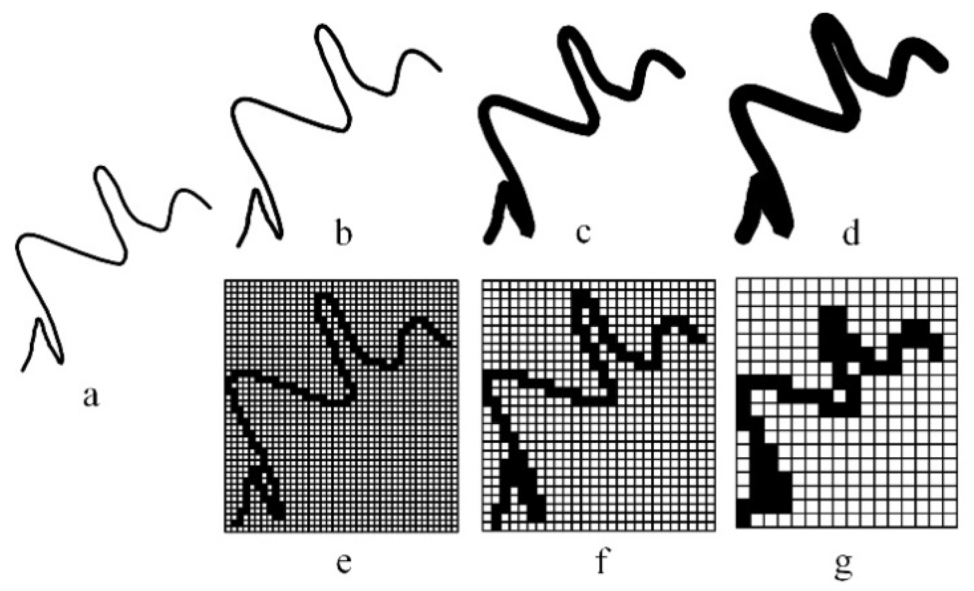
Consistency evaluation of map LoD can be conducted at both the semantic and representational levels of a geometric graph. Touya et al. [8] divided building polygons in OpenStreetMap into four hierarchy levels (single building, street, city, and country) according to different LoD hierarchies under different scales. As another example, considering features representing forest areas and single buildings, these features belong to different semantic levels: a forest area that has few vertices and overlaps several buildings should be considered inconsistent at the semantic level [9,10]. The most direct method of measuring the LoD of a geometric element is to calculate the shortest distance between adjacent points belonging to the feature. For example, Ai [11] measured the LoD of a point cluster using a point-oriented Delaunay triangle. For a curve or polygon feature, the length of the shortest side of the feature can be used as the minimum detail parameter for cartographic representation [12]. For the sake of clarity and readability, curve symbols on a map have a minimum perceptible width. The larger the scale, the larger the ground distance to which the line width corresponds. When the scale is less than a certain threshold value, neighboring parts of the feature will aggregate. This means that the curve symbol width of curves at aggregation can be used as a parameter for LoD assessment [12,13]. This method is called incremental curve detail detection. Another method involves rasterizing curve features using incremental grid widths. When the grid width is greater than a threshold value, the part of the curve that does not coalesce at smaller grid widths appears to aggregate. The grid size which is equal to the threshold value is used to define the LoD of a curve [14]. Figure 1 shows the LoD detection processes employed by the aforementioned methods. In Figure 1b, the curve detail is clear when the symbol width is 1m; however, the symbol aggregates once and twice when its width is 2 m (Figure 1c) and 3.5 m (Figure 1d), respectively. Figure 1e–g show the same curve rasterized with different grid widths. Results obtained by the increment grid width method are consistent with those obtained by the increment symbol width method. The LoD parameter of a feature can be measured by the threshold width (symbol width or grid width) where parts of the feature conglomerate together.
This paper presents a method that uses computational geometry to detect the minimum graphical units of map features and computes LoD parameters using a mathematical statistics model. This model estimates the actual map scale and its deviation from map-nominal scale and evaluates the level of detail consistency of map feature representations. The method obtains the LoD and feature representation by detecting topology conflict in curve-oriented representations on the basis of the internal consistency principle, which needs to be visualized several times with different parameters. The method presented in this paper allows us to recognize the minimal representation graphical unit and to calculate the LoD of map features using the graphical unit. Compared with previous methods, our algorithm uses mathematical models while the former uses analog detection.
The structure of this paper is as follows. In Section 2.1, we present techniques to detect the basic graphical units of contour lines and artificial map features. Section 2.2 presents a statistical method to calculate the LoD of each feature and evaluate the LoD consistency of multiple features. In Section 3, we design an experiment to test the proposed method and analyze the experimental results. Section 4 summarizes the paper and prospects for future work.
2. Methods
2.1. Graphical Unit and LoD
It is natural to describe the LoD of a geographical feature using its geometric details. For the geographical features represented by different geometries, the representations of their geometric details are quite different. For a polyline, the bends in it could reflect its geometric details. It is obvious that the smaller the bends are, the richer its geometric details will be. Herein, we call the geometry of the geographical feature which could reflect its geometric detail degree the graphical unit. Thus, the bend could be the graphical unit of a curve.
2.1.1. Bend of Curve as Graphical Unit
For a digital map, in order to meet the aesthetic requirements of feature representation, cartographic features commonly contain redundant points, so the line segment of a feature cannot be regarded as its graphical unit. According to the above discussion, a bend is regarded as a good graphical unit for the curve feature. However, it is not an easy task to describe and detect the bends of a curve. Scholars have provided various detection bend approaches for a curve [15,16,17,18]. Ai [15] used a Delaunay triangle net to build a curve-bending binary tree structure, allowing them to interpret the nested curve relationship and effectively extract a graphical unit, called leaf bend.
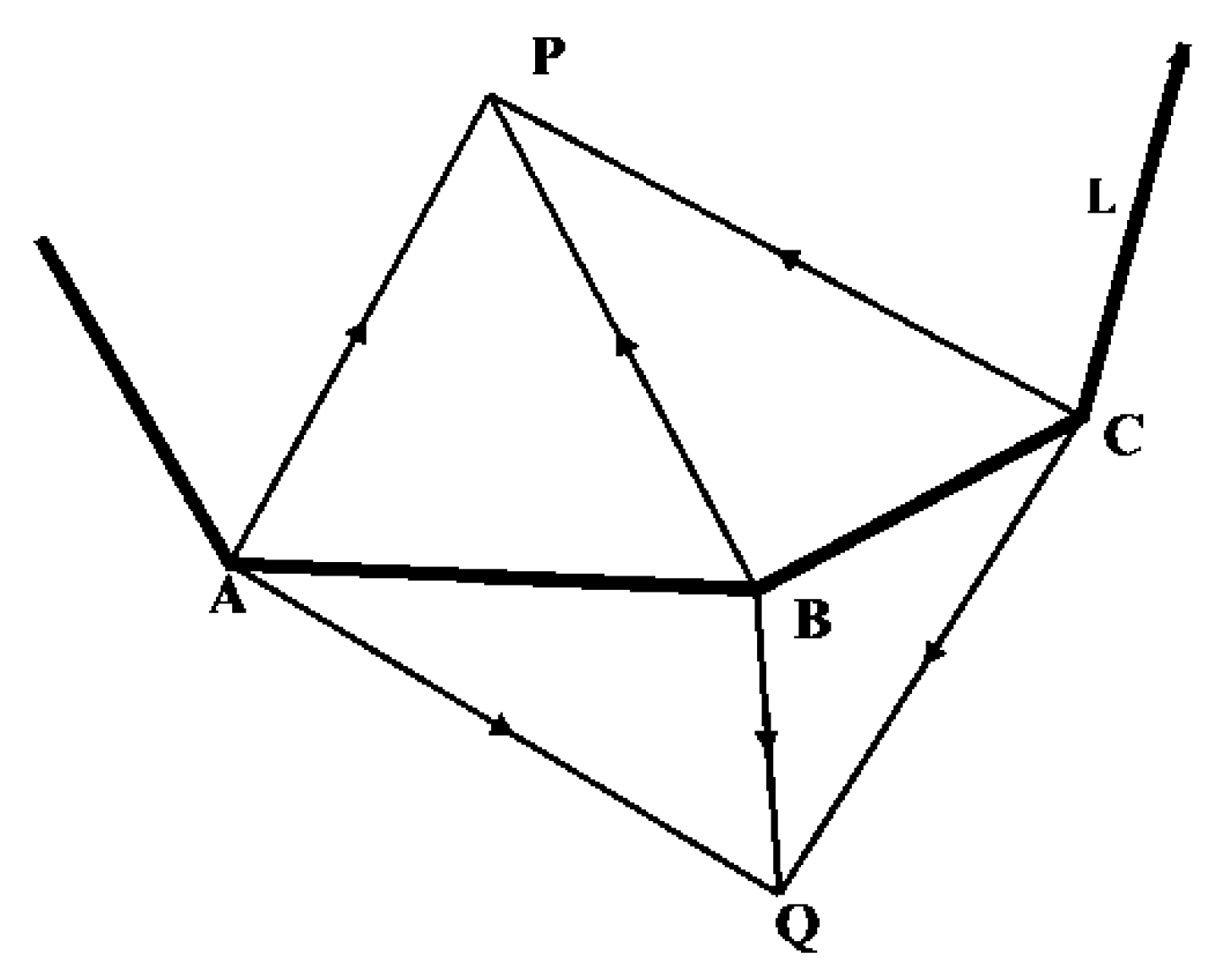
Herein, we use the method proposed in [15] to detect the bends of a curve. The points on the curve can be set up as a constrained triangle network with the curve as the constraint edge [19,20]. By extracting the left and right triangle network, we can build the tree structure of the left and right bends. The process is shown in (a–h) in Figure 2. For the curve shown in Figure 2a, the points on the curve are used to build a constrained Delaunay triangle network (Figure 2b). Two steps are used to decide whether a triangle is on the left or right side of a curve. Firstly, the order of the three points of a triangle is adjusted according to their location along the curve. Taking the triangle in Figure 3 as an example, the adjusted order will be A, B, and P. Secondly, the vector product of and is calculated as shown in Equation (1); if V > 0, the triangle is on the left side of the curve; if V < 0, it is on the right side. If V = 0, the three points A, B, and P are on the same line. Figure 3 shows the processes involved in these operations.
where and are regarded as space vectors which have three components and the value of the third component is 0, e.g., , and refers to the cross product of two space vectors.
According to Equation (1), the triangles in Figure 2b are divided into two sets: left-side triangles and right-side triangles. Figure 2c,d represents the subsets of left and right triangles. To detect whether the triangle subsets are on the left or right side and their nesting relationship, we first detect the entrance point of the first-level curve from the starting point of the curve.
If this point is not the vertex of a triangle, the next point will be considered until a point belongs to a triangle, and this is used as the starting point. For all the triangle edges containing the starting point, select the one that is connected with the point with the largest number. The point with the largest number is called the ending point. Next, the part of the curve between the starting point and the ending point is taken as one of the first-level bends; the ending point is the starting point of the next bend. We repeat this operation to get the next bend of the first level, and so on, until the end of the curve. For the right bend (Figure 2d), the first-level bends cover points 7–22, 22–39, 41–48, 49–72, and 73–80; on the left, the first-level bend covers points 0–80 (all the points on the curve). For the right bends, there is also a first-level bend which covers points 0–80, as shown in Figure 2g. For all bends under the first bends, we build up a bend binary tree according to the method proposed by Ai [14]. The bend tree structures of the left and right sides are shown in Figure 2g,h, and the left and right leaf bends are shown in Figure 2e,f.
2.1.2. Graphical Unit of Natural Features
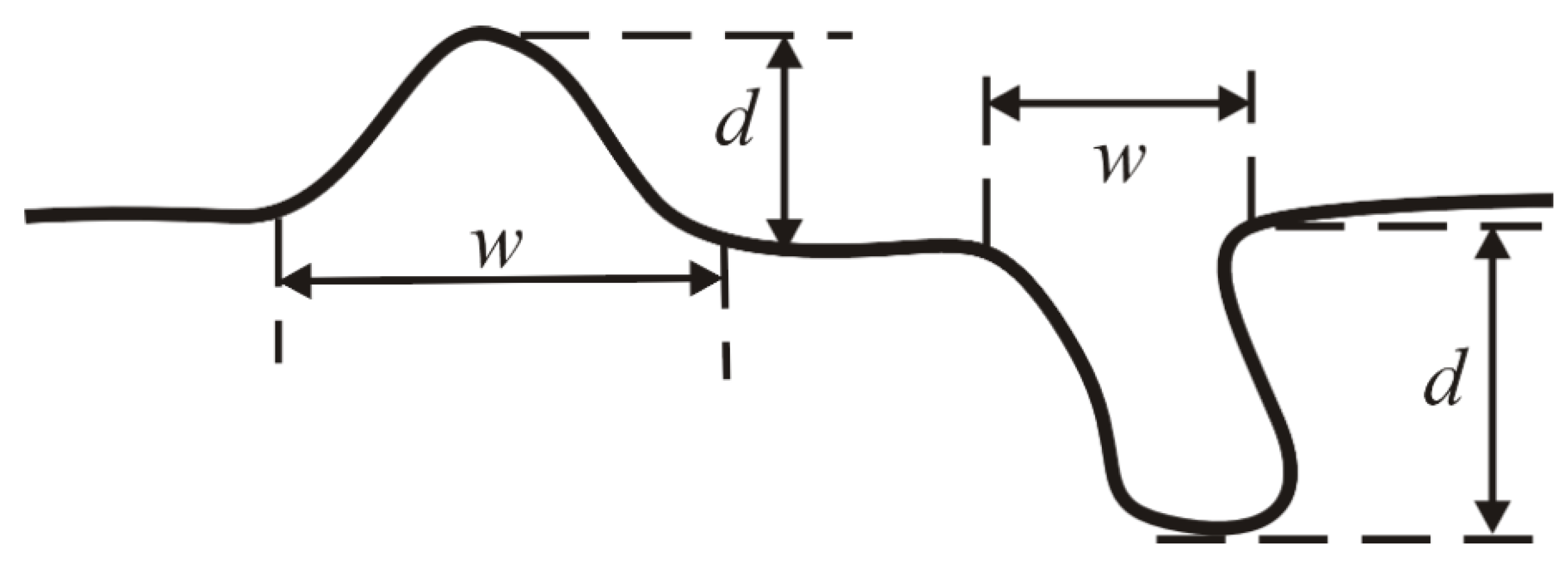
Herein, we take the minimum width and depth of the leaf bends as the parameter of the natural features’ graphical unit. The line segment from the starting point to the ending point of the bend forms a bend base, the distance of it is the width (w) of the bend, and the largest distance from the inner points of the bend to its base is the depth of the bend(d) (Figure 4). The smaller of the width and depth values is regarded as the LoD parameter of the bend. We use the relationship between the minimum distinguishable distance (0.3 mm in most cases in this paper) [21] and the LoD parameters to calculate a scale value to which each bend corresponds (Equation (2)). The calculated scale is called the actual scale of the bend.
where is the actual scale denominator (as opposed to the nominal scale denominator); is the LoD parameter (measured in meters), and is the minimum distinguishable distance (in millimeters; typically, 0.3). In general, for maps with a scale greater than 1:10,000, it is better to take 0.3mm as the value. For maps with a smaller scale, due to the large amount of data and more complicated degree of curvature, the value of can be adjusted to adapt to this trend. Therefore, for maps with a scale less than 1:100,000 and greater than 1:1,000,000, we set the value of to 0.6mm, and for maps with a scale less than 1:1,000,000, we set the value of to 1mm. The LoD parameters of all the leaf bends provide the data for the statistical analysis of the curves’ LoD in Section 2.2. The LoD parameter calculation model based on the structure of a curve is consistent with the incremental LoD detection approach.
2.1.3. Graphical Unit of Humanmade Features
Humanmade features tend to have regularly geometric shapes. Each side of a building polygon is approximately parallel or orthogonal to another side of the building. The LoD of such a building polygon can be measured by regular graphical units (such as convexity, concavity, stair, and gap). These units can easily be identified using computational geometry techniques.
The approaches to identifying building polygon basic graphical units exist mostly in the references on geographical generalization. For example, Xu and Long identified the local model constructed by the continuous four points of a building polygon [22]; Samsonov and Yakimova [23] recognized the partial characteristic model by using the orthogonality of continuous sides and length differentiation for line features, and then proposed respective simplification strategies for different models in map generalization. Wang and Lee [24] and Wang et al. [25] summarized building polygon partial pattern recognition methods that are based on the relationships between sides and angles.
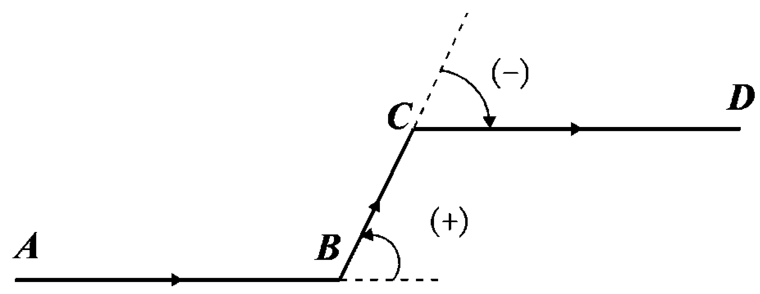
Herein, we suggest some partial models for building polygon identification based on polygon characteristics such as angles between continuous sides and side length variations. In the calculation of the included angles between two continuous sides, we consider clockwise to be negative and counterclockwise to be positive (angles range from −90to 90°). In Figure 5, we calculate the included angles of vector quantities , and . The included angle formed anticlockwise from to is positive, and the included angle formed clockwise from to is negative. Using the included angles constructed by continuous sides and the length differentiation of the continuous sides, the identification of the partial graphical unit of a polygon can be obtained. Table 1 lists the conditional descriptions and methods for various graphical units; the fifth column provides detailed parameter values for different graphical units of building polygons.
2.2. Minimum Representative Scale
To calculate the minimum representative size of a feature, we must construct a dataset for geographical features (including natural and artificial features) on some scales, identify the minimum graphical units by using the approach detailed in Section 2.1, and calculate the LoD parameters of each graphical unit. For natural curve features, which include abundant basic graphical units (leaf bends), the smallest leaf bend theoretically represents the most detailed level. Due to the need for smooth and aesthetic representation, redundant points are often included in natural curve features. In a map, very few parts of the curve converge together and are visually acceptable. In this section, we calculate the minimum representative scale for a set of leaf bends using mathematical statistics.
The process we use to calculate the minimum representative scale consists of the following steps. First, we divide the LoD parameters for all the leaf bends of each curve into quartiles. Identifying the three levels of parameters as Q1, Q2, and Q3, we calculate the average value of all parameters smaller than the lower quartile point (Q1) and use this value as the LoD parameter of the curve feature. Next, we eliminate outliers (normally, greater than Q3 + 1.5 ∗ (Q3 − Q1) or less than Q1 − 1.5 ∗ (Q3 − Q1)). Following this, we can calculate the LoD parameter and estimate the actual scale of a curve using Equation (2). If the nominal scale of the map is known, we can compare it with the actual scale. For each curve, the average value of the LoD parameter is used to evaluate the overall detail level of all features. The standard deviation of the detail parameter can be used to differentiate the detail levels among different curves in the dataset. When the number of leaf bends of a curve is not large enough, we can combine the leaf bends of all the curves and calculate the average value of all parameters below the lower quartile point (Q1). This average value can be used as an overall LoD parameter for this kind of curve.
Because basic graphical units are not abundant in polygons depicting artificial features such as buildings, it is inappropriate to analyze the LoD parameter for each feature. Instead, we analyze the basic graphical unit parameters of all building polygons, eliminate outliers, and calculate the average value (Ave) and mean square error (δ) of all parameters for the lower quartile point (Q1). The average value can be a LoD parameter for this batch of building polygons. After we determine the actual scale of the building polygons (1:), we can compare it to the nominal scale (1:). We must set an allowed scale variation threshold value t (0 < t < 1; t = 0.1 in this paper). When the actual scale meets the criterion, it is considered consistent with the nominal scale.
The mean square error, δ, can be used to describe LoD consistency. The greater the mean square error is, the greater the difference in the LoDs among the features will be. When δ is less than or equal to 20% of the average value (), the LoD can be considered consistent. If δ is greater than 20% of the average value and less than or equal to 30% of the average value (i.e., ), consistency is considered moderate. If δ is greater than 30% of the average value (i.e., ), consistency is poor.
3. Experiment and Analysis
3.1. Contour Lines
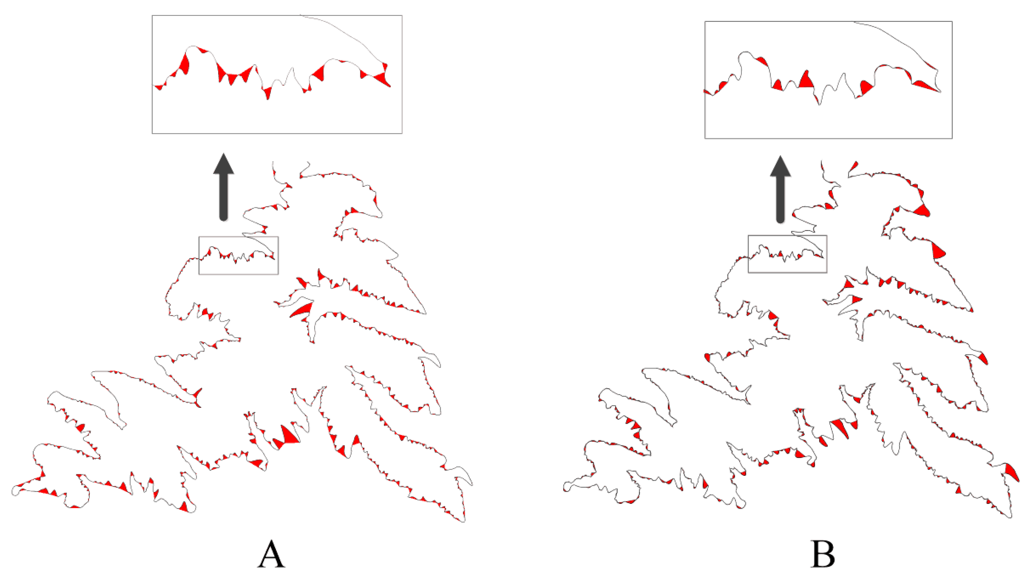
For our analysis, we selected 50 contour lines from a 1:5K topographical map. Table 2 provides the basic descriptions for six of them. We constructed bend-level trees, obtained all the leaf bends, and calculated the LoD parameter for each curve. In Figure 6, the Figure 6A,B show the left and right leaf bends of the No.6 contour line with some close-ups in the rectangles. Table 3 lists the corresponding parameters for the left and right leaf bends of the curve. In the table, ‘l’ is the LoD parameter.
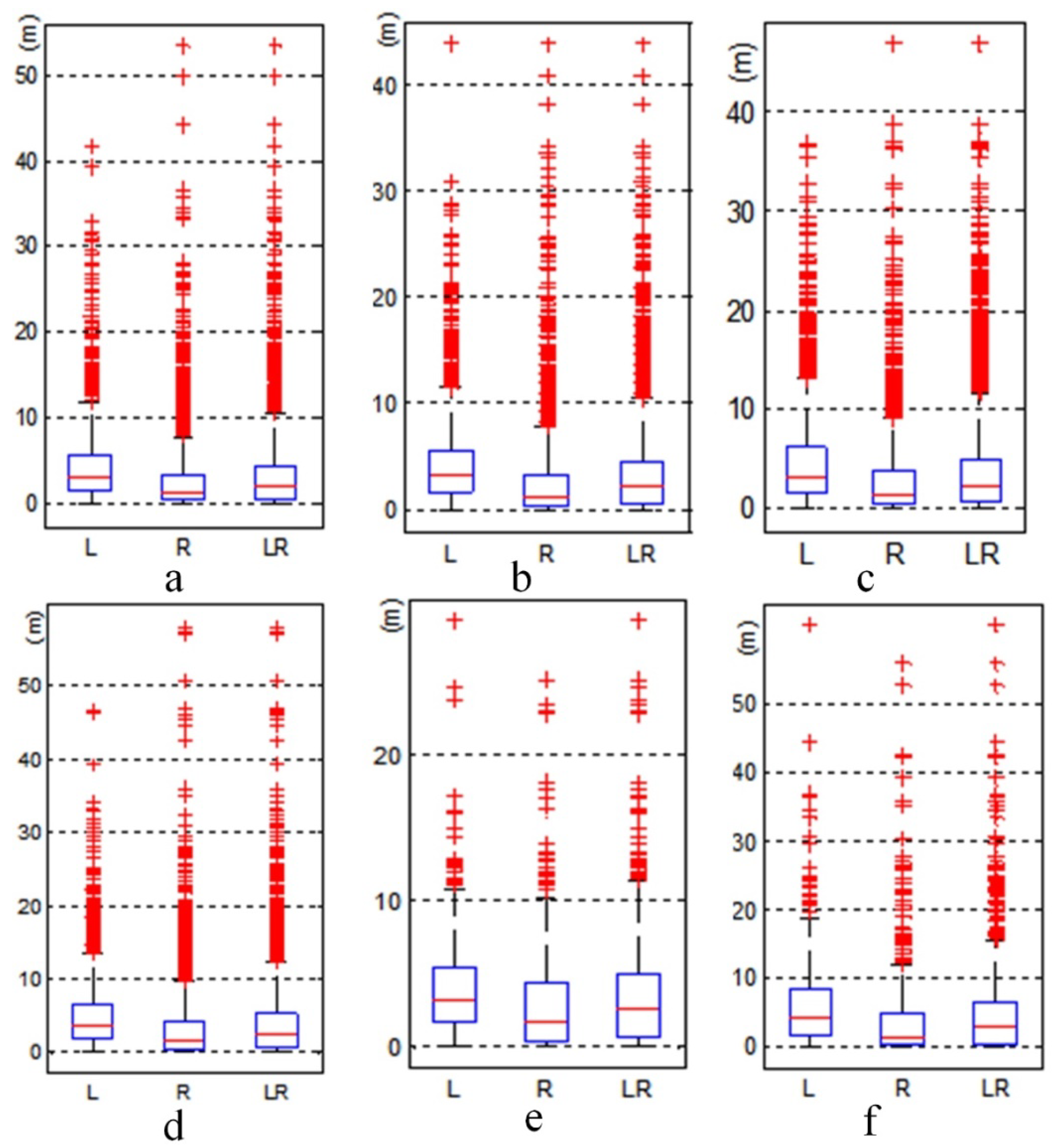
In Figure 7a–f, L, R, and LR correspond to the box plots of left bends, right bends, and all bends, respectively. The “+” signs in the figure represent outliers. Figure 7 shows that there is a large range in the median of the detail level parameters among the six contour lines. It also illustrates the necessity of considering both left and right bends to evaluate the detail level of a curve.
Figure 8 is the boxplot of all of the bends (left and right) of six curves after removing outliers. This figure shows the lower quartile of the leaf bend parameter of each curve is around 2.0 m. We used the average value of all parameters under the lower quartile of each curve as its LoD parameter. The third row in Table 4 shows the calculated scale for each curve. Note that the nominal scale and those calculated for the 5th, 6th, 8th, 22nd, 26th and 30th curves are inconsistent. The average detail parameter of the 50 curves is 1.554 m, with a mean square error δ of 0.105 m. Because this mean square error value is less than 20% of the average (i.e., ), we consider the LoD of the curve highly consistent.
3.2. Buildings
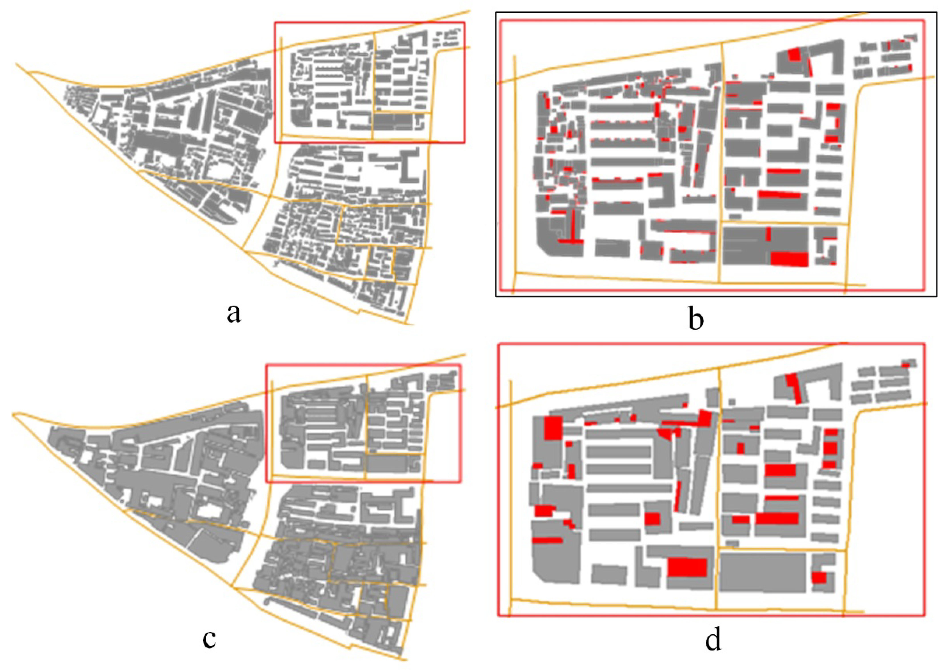
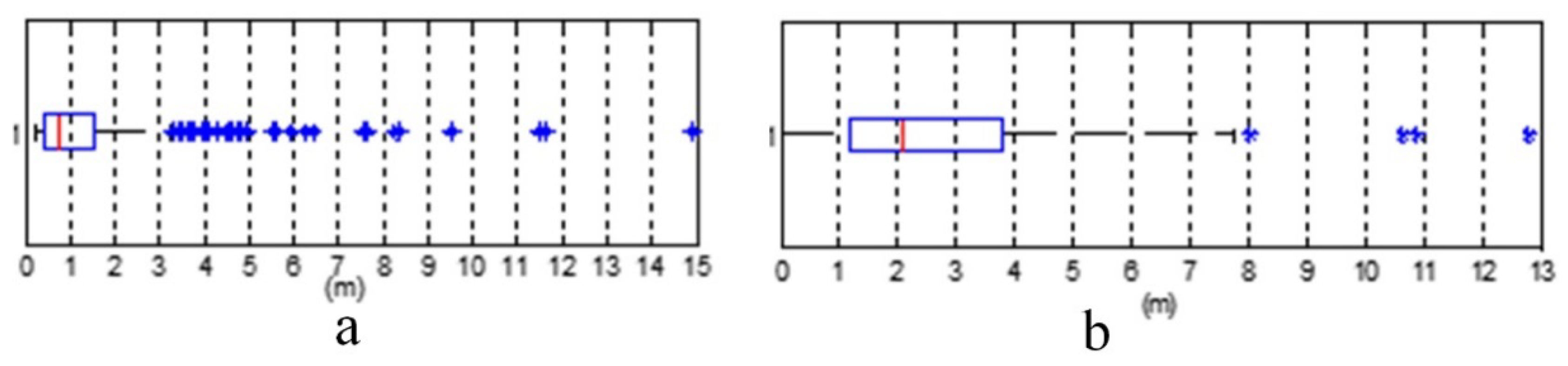
Given two maps of the same region of a city, one having a scale of 1:2K and the other of 1:5K, we selected an area of 17,500 m2 for our experiment. Figure 9a shows the 1:2K experimental area, where we detected the basic graphical unit of the building polygon utilizing the approach detailed in Section 2.1.3. Figure 9b shows the details of an area corresponding to the red box in Figure 9a. Each red solid area represents the smallest graphical unit detected. Figure 9d shows the results detected for the same area from the 1:5K map. Using the quartile method described in Section 2.2, we analyzed the data for these two different scales (Figure 10). The mean LoDs for the building polygons on the 1:2K map is 0.55 m. Given a map distance of 0.3 mm, we determined that the actual map scale is 1:1850 for the 1:2K map. In contrast, the LoD for the 1:5K map is 1.350 m, and its actual scale 1:4500. The two actual scales are both within the tolerance range of the map scales.
3.3. Scale Inconsistency Detection
As for the whole map in VGI data, some geographic features that are not consistent with the actual scale may be mixed into the map data uploaded by volunteers, resulting in the phenomenon that the geospatial information does not match the real map scale. The method proposed in this paper can detect the scale inconsistency caused by the large-scale data in the small-scale map. For the detection of natural geographical features, in the first step, we selected some river elements in Sichuan Province of China with a nominal scale of 1:2,000,000 as the original data, and obtained the left leaf detail level parameters and right leaf detail level parameters contained in each river, respectively, then calculated the map scale corresponding to the actual situation after integration; the second step was to select the river data of the same area with a nominal scale of 1:750,000 as the “wrong data” and select some of them to replace the original data with a scale of 1:2,000,000, so that the mixed data could be considered as the VGI data uploaded by volunteers; in the last step, we calculated the actual map scale of the mixed data, and compared it with the results in the first step. Figure 11 demonstrates the experimental data.
Through the analysis of the results in Table 5, it can be found that the nominal scale of the original map is 1:2,000,000, which is close to the actual calculated scale of 1:1,997,362. When some large-scale geographic features are mixed into the original map, the level of detail in the map will change to a large extent, resulting in the reduction of the level of detail parameter l. Therefore, the actual scale of the mixed map calculated by the method in this paper will also change greatly, from 1:1,997,362 to 1:819,442, so this method can be used to detect the scale inconsistency in natural geographical features.
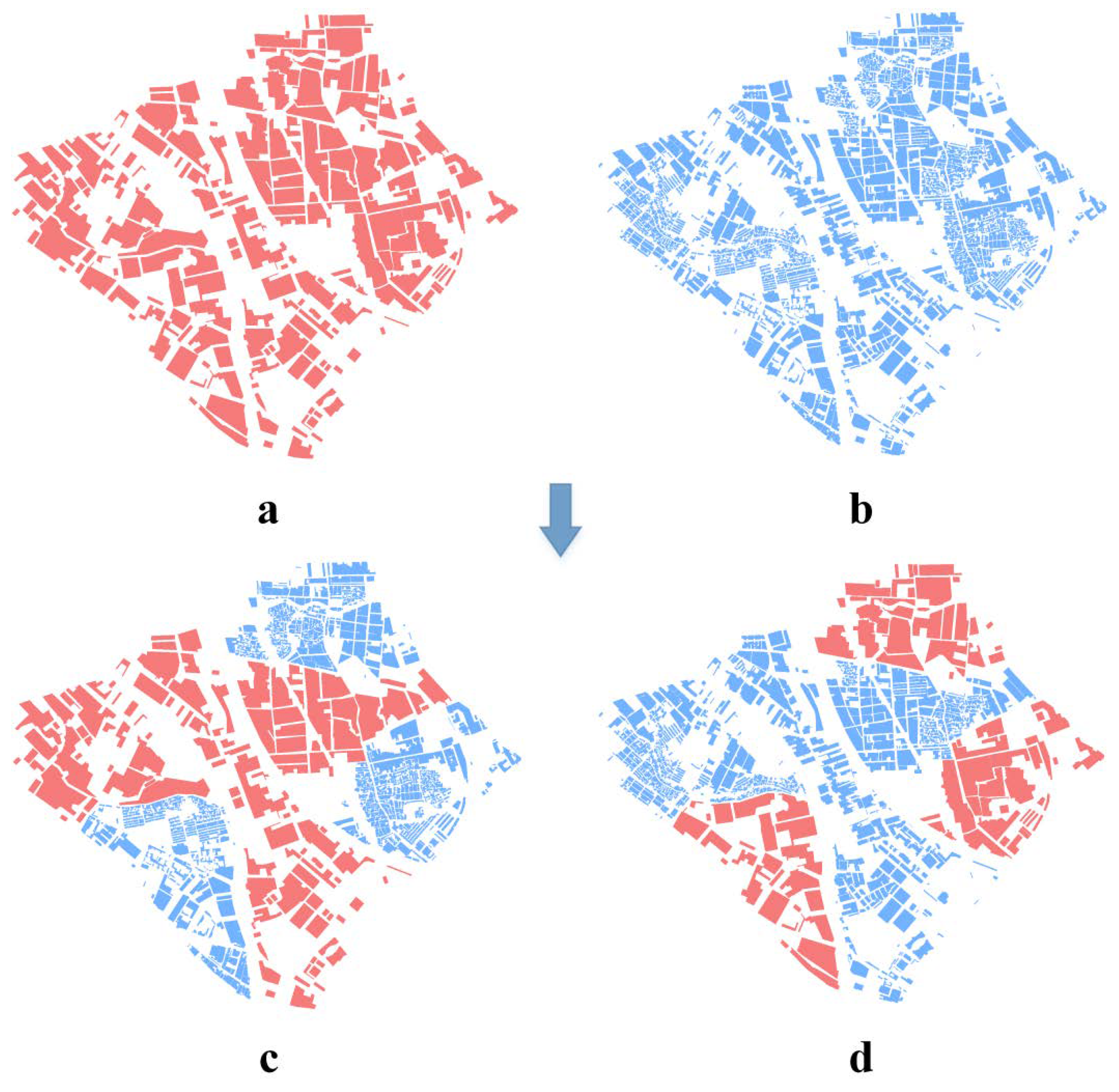
For the detection of building scale inconsistency, we chose a building group in a certain area of China with a scale of 1:30,000 as the original data. The procedure was the same as that of the natural geographic element detection. Firstly, the actual map scale was calculated by the detail level parameters of the left and right leaves of each building; secondly, large-scale map data with a nominal scale of 1:10,000 was selected to replace the buildings in the scale of 1:30,000; finally, the actual scale of the “VGI like data” was calculated.
The experimental results are the same as those of the natural geographical features, and the data obtained in Table 6 prove that the method has a good discrimination effect on the inconsistency of building scale in the map. For the original building map, the nominal scale is 1:10,000, and the calculated scale is 1:9339; these are close to each other. When some buildings from the large-scale map are mixed into the original map, the actual scale of the map is increased from 1:9339 to about 1:2600, resulting in an inconsistent map scale.
4. Conclusions
Previous research on spatial data quality has focused primarily on integrity [26,27], position accuracy [28,29], attribute accuracy, shape similarity [30], and some other aspects [31]. These studies have rarely focused on LoD consistency. Given the ubiquity of data collection and the diversification of data processing, maps are often produced using various data and a wide range of data processing methods for a wide range of purposes. In order to ensure that a map is an objective and scientific representation of the observable world, consistency analysis on data LoD is critical. To perform this analysis and resolve LoD inconsistencies, users must calculate the actual representative scale of map features and then classify or process map features based on the LoD. This will ensure that the scale deviation of map features is within tolerance limits.
Consistency evaluation of the LoD for digital map products is also a vital part of the quality control process. This paper presents a method for detecting the basic graphical units of different geographical features using both computational geometry and statistics. From these graphical units, we can obtain feature LoDs and assess the deviation of the LoD from a nominal scale to measure its consistency. The method proposed in this paper is based on the map relationship between distinguishable distance and its minimum graphical unit, with consideration of human visual limitations.
Furthermore, this method works well for both natural linear features and building polygons. However, it is worth noting that we cannot use the method in this paper to evaluate the inconsistency of geographical features in all cases. This is because, for some physical geographical features, such as smooth slopes in high mountains and transition zones between rock terrain, there may be a situation where smooth and rugged contours exist at the same time. In this case, the inconsistency of LoD can actually reflect the characteristics of the objective world very well. Therefore, in the next research process, we need to make some improvements to the methods in this paper, so that physical geographical features that can reflect the actual geographical features well will not in fact be judged as an LoD inconsistency. Besides, we need to further study the definition of the basic graphic units of other types of features and the detection of their shapes and try to select different statistical models to achieve the calculation of the comprehensive LoD parameters of massive data sets, so as to achieve the detection of map inconsistency on the big data scale.
Author Contributions
Formal analysis, Jia Xiao; resources, Pengcheng Liu; writing—original draft, Pengcheng Liu; writing—review and editing, Jia Xiao. All authors have read and agreed to the published version of the manuscript.
Funding
This research was funded by the Fundamental Research Funds for the Central Universities, grant number CCNU30106190454 and Open Research Fund Program of Key Laboratory of Digital Mapping and Land Information Application Engineering, grant number ZRZYBWD201909.
Conflicts of Interest
The authors declare no conflict of interest.
References
- Girres, J.F.; Touya, G. Quality Assessment of the French OpenStreetMap Dataset. Trans. GIS 2010, 14, 435–459. [Google Scholar] [CrossRef]
- Haklay, M. How good is volunteered geographical information? A comparative study of OpenStreetMap and Ordnance Survey datasets. Environ. Plan. B Plan. Des. 2010, 37, 682–703. [Google Scholar] [CrossRef] [Green Version]
- Goodchild, M.F.; Li, L. Assuring the quality of volunteered geographic information. Spat. Stat. 2012, 1, 110–120. [Google Scholar] [CrossRef]
- Hung, K.C.; Kalantari, M.; Rajabifard, A. Methods for assessing the credibility of volunteered geographic information in flood response: A case study in Brisbane, Australia. Appl. Geogr. 2016, 68, 37–47. [Google Scholar] [CrossRef]
- Zhao, Y.J.; Zhou, X.G. Version similarity-based model for volunteers’ reputation of volunteered geographic information: A case study of polygon. Acta Geod. Cartogr. Sin. 2015, 44, 578–584. [Google Scholar] [CrossRef]
- Stehman, S.V.; Fonte, C.C.; Foody, G.M.; See, L. Using volunteered geographic information (VGI) in design-based statistical inference for area estimation and accuracy assessment of land cover. Remote Sens. Environ. 2018, 212, 47–59. [Google Scholar] [CrossRef] [Green Version]
- Schultz, M.; Voss, J.; Auer, M.; Carter, S.; Zipf, A. Open land cover from OpenStreetMap and remote sensing. Int. J. Appl. Earth Obs. Geoinf. 2017, 63, 206–213. [Google Scholar] [CrossRef]
- Touya, G.; Brando-Escobar, C. Detecting level-of-detail inconsistencies in volunteered geographic information data sets. Int. J. Geogr. Inf. Geovis. 2013, 48, 134–143. [Google Scholar] [CrossRef] [Green Version]
- Brando, C.; Bucher, B.; Abadie, N. Specifications for user generated spatial content. In Advancing Geoinformation Science for a Changing World; Geertman, S., Reinhardt, W., Toppen, F., Eds.; Springer: Berlin/Heidelberg, Germany, 2011; pp. 479–495. [Google Scholar]
- Duchêne, C.; Christophe, S.; Ruas, A. Generalisation symbol specification and map evaluation: Feedback from research done at COGIT laboratory, IGN France. Int. J. Digit. Earth 2011, 4 (Suppl. 1), 25–41. [Google Scholar] [CrossRef]
- Ai, T.; Liu, Y. A method of point cluster simplification with spatial distribution properties preserved. Acta Geod. Cartogr. Sin. 2002, 31, 175–181. [Google Scholar]
- Ai, T.; Li, Z.; Liu, Y.; Zhou, Y. The Changes Accumulation Model for Streaming Map Data Transferring over Web. Acta Geod. Cartogr. Sin. 2009, 38, 514–519. [Google Scholar]
- Huang, Y.; Ai, T.; Liu, H. The detection and removal of conflicts in road network generalization by Delaunay triangulation. In Proceedings of the 2009: 17th International Conference on Geoinformatics, Fairfax, VT, USA, 12–14 August 2009; IEEE: Fairfax, VA, USA, 2009; pp. 1–6. [Google Scholar] [CrossRef]
- Cheng, X.; Wu, H.; Ai, T.; Yang, M. Detail Resolution: A New Model to Describe Level of Detail Information of Vector Line Data. In Spatial Data Handling in Big Data Era. Advances in Geographic Information Science; Zhou, C., Su, F., Harvey, F., Xu, J., Eds.; Springer: Singapore, 2017; pp. 167–177. [Google Scholar]
- Ai, T. The drainage network extraction from contour lines for contour line generalization. ISPRS J. Photogramm. Remote Sens. 2007, 62, 93–103. [Google Scholar] [CrossRef]
- Qian, H.Z.; Wu, F.; Chen, B.; Zhang, J.H.; Wang, J.Y. Simplifying line with oblique dividing curve method. Acta Geod. Cartogr. Sin. 2007, 36, 443–456. [Google Scholar]
- Guo, Q.S.; Huang, Y.; Zhang, L. The Method of Curve Bend Recognition. Geomat. Inf. Sci. Wuhan Univ. 2018, 33, 596–599. [Google Scholar]
- Liu, P.; Yang, W.; Li, C. Multi-branch tree model of bend for curve and its application in map generalization. Appl. Res. Comput. 2012, 29, 2793–2795. [Google Scholar]
- Lee, D.T.; Lin A, K. Generalized Delaunay triangulation for planar graphs. Discret. Comput. Geom. 1986, 1, 201–217. [Google Scholar] [CrossRef] [Green Version]
- Fang, T.P.; Piegl, L.A. Algorithm for constrained Delaunay triangulation. Vis. Comput. 1994, 10, 255–265. [Google Scholar] [CrossRef]
- Li, Z.; Openshaw, S. Algorithms for automated line generalization based on a natural principle of objective generalization. Int. J. Geogr. Inf. Syst. 1992, 6, 373–389. [Google Scholar] [CrossRef]
- Xu, W.; Long, Y.; Zhou, T.; Chen, L. Simplification of Building Polygon Based on Adjacent Four-Point Method. Acta Geod. Cartogr. Sin. 2013, 42, 929–936. [Google Scholar]
- Samsonov, T.E.; Yakimova, O.P. Shape-adaptive geometric simplification of heterogeneous line datasets. Int. J. Geogr. Inf. Sci. 2017, 31, 1485–1520. [Google Scholar] [CrossRef]
- Wang, Z.; Lee, D. Building Simplification Based on Pattern Recognition and Shape Analysis. In Proceedings of the China 2000: 9th International Symposium on Spatial Data Handling, Beijing, China, 10–12 August 2000; pp. 58–72. [Google Scholar]
- Wang, H.; Wu, F.; Zhang, L.; Deng, H. The application of mathematical morphology and pattern recognition to building polygon simplification. Acta Geod. Cartogr. Sin. 2005, 34, 269–276. [Google Scholar]
- Cai, A.; Zha, L.; Liu, D.; Gu, L. Analysis of Synthetical Multi-fuzzy Evaluation on the Quality of GIS Data. Geo-Inf. Sci. 2005, 7, 50–53. [Google Scholar]
- Deng, M.; Fan, Z.D.; Liu, H.M. Performance Evaluation of Line Simplification Algorithms Based on Hierarchical Information Content. Acta Geod. Cartogr. Sin. 2013, 42, 443–456. [Google Scholar]
- Zhang, X.; Guo, T.; Tang, T. An Adaptive Method for Incremental Updating of Vector Data. Acta Geod. Cartogr. Sin. 2012, 41, 613–619. [Google Scholar]
- Chen, B.; Zhu, K.; Xue, B. Quality Assessment of Linear Features Simplification Algorithms. J. Geomat. Sci. Technol. 2007, 24, 121–124. [Google Scholar]
- Liu, P.; Luo, J.; Ai, T.; Li, C. Evaluation Model for Similarity Based on Curve Generalization. Geomat. Inf. Sci. Wuhan Univ. 2012, 37, 114–117. [Google Scholar]
- Zhang, J.; Goodchild, M.F. Uncertainty in Geographical Information; CRC Press: Boca Raton, FL, USA, 2002. [Google Scholar]
Figure 1.
Detecting the LoD of a curve using the progressive increment method. (a) A curve with bends. (b–d) Curve representation when the symbol width is respectively 1m, 2m and 3.5m. (e–g) Rasterizing results of curves, respectively, at 1m, 2m and 3.5m.
Figure 1.
Detecting the LoD of a curve using the progressive increment method. (a) A curve with bends. (b–d) Curve representation when the symbol width is respectively 1m, 2m and 3.5m. (e–g) Rasterizing results of curves, respectively, at 1m, 2m and 3.5m.

Figure 2.
The process for identifying the graphical units of a curve. (a) An example curve with the order number of points on the curve. (b) Delaunay triangulation constructed with the curve points. (c) The triangulation sets on the left side of the forward direction of the curve. (d) The triangulation sets on the right of the forward direction of the curve. (e) The left-bend sets on the left of the forward direction of the curve. (f) The right-bend sets on the left of the forward direction of the curve. (g) The hierarchical structure of the left-side curve. (h) The hierarchical structure of the right-side curve.

Figure 3.
Judging the position of Point P, Q relative to the curve L.

Figure 4.
The schematic map of the width (w) and depth (d) of a bend.

Figure 5.
Schematic map of the size and direction of the intersection angle.

Figure 6.
The (A) and (B) leaf bends and four close-ups along the No. 6 contour line in Table 1.
Figure 6.
The (A) and (B) leaf bends and four close-ups along the No. 6 contour line in Table 1.

Figure 7.
Boxplots of the LoD parameters based on the left bends, right bends, and all bends for six contour lines (the “+” symbol represents abnormal values). (a) Boxplot of the LoD parameters for the No.1 contour line. (b) Boxplot of the LoD parameters for the No.1 contour line. (c) Boxplot of the LoD parameters for the No.3 contour line. (d) Boxplot of the LoD parameters for the No.4 contour line. (e) Boxplot of the LoD parameters for the No.5 contour line. (f) Boxplot of the LoD parameters for the No.6 contour line.

Figure 8.
Boxplots of the LoD parameters based on the leaf bends of the six curves (after removing the outliers).
Figure 8.
Boxplots of the LoD parameters based on the leaf bends of the six curves (after removing the outliers).

Figure 9.
Building polygon experimental data and detected graphical units. (a) 1:2K building polygon data. (b) Graphical units within the red box in Figure 9a. (c) 1:5K scale building polygon data. (d) Close-up of graphical units within the red box in Figure 9c.

Figure 10.
Boxplot of LoDs for the building polygons from 1:2K (a) and 1:5K (b) maps.

Figure 11.
Replacing some large-scale geographic features into a small-scale map. (a) Original small-scale map. (b) Mixed map. (The red polylines are the original small-scale geographic features with a scale of 1:2,000,000; the blue polylines represent “Wrong Data” on a large scale, with a scale of 1:750,000).

Figure 12.
Replacing some large-scale buildings into a small-scale map. (a) Original small-scale buildings. (b) Large scale buildings for replacement. (c) Mixed map 1. (d) Mixed map 2. (The red polygons represent the original small-scale geographic buildings with a scale of 1:30,000, the blue polygons represent “Wrong Data” on a large scale, with a scale of 1:10,000).


Table 1.
Graphical units, identification methods and LoD parameters of artificial building polygons.
Table 1.
Graphical units, identification methods and LoD parameters of artificial building polygons.
| No. | Pattern | Example | Regularity | Minimal Detail Distance (d) |
|---|---|---|---|---|
| 1 | convex |  | The signs of the middle four consecutive turning angles are positive, negative, positive and negative; their angle value is approximately 90 degrees, and the angles of vector 12 and vector 56 are close to 0 degrees. | The minimal detail distance is the shorter length of edge 23 and edge 34, i.e., d = MIN(d23, d34), where d23 and d34 are the lengths of edge 23 and edge 34, respectively. |
| 2 | concave |  | The signs of the middle four consecutive turning angles are negative, positive, positive and negative; their angle value is approximately 90 degrees, and the angles of vectors 12 and 56 are close to 0 degrees. | The minimal detail distance is the shorter length of edge 23 and edge 34, i.e., d = MIN(d23, d34). |
| 3 | notch |  | The signs of the four consecutive turning angles are negative, positive, negative, negative or positive, negative, positive, positive; their angle value is approximately 90 degrees, and edges 12 and 23 are short edges. | The minimal detail distance is the shorter edge length of the notch, i.e., d = MIN(d12, d23). |
| 4 | multiple-step stair |  | The four consecutive turning angles’ values are approximately 90 degrees, the symbols are alternating, and edges 23 and 45 are short edges (i.e., the middle edges all are short edges). | The minimal detail distance is the shortest edge’s length, i.e., d = MIN (d12, d23, d34, d45). |
| 5 | spike |  | The angle between vector 12 and vector 34 is approximately 0 degrees, edges 23 and 34 are short edges, and the angle between vector 12 and vector 34 is an acute angle. | The minimal detail is the shorter edge length of the acute angle, i.e., d=min(d23, d34) |
| 6 | Dull corner |  | The angle between vector 12 and vector 34 is an acute angle, edge 23 is the short edge, and edges 12 and 34 are long edges. | d= d23 |
| 7 | Curve steps |  | The overall shape is a ladder above the sector; the four consecutive turning angles’ values are approximately 90 degrees. | The minimum detail distance is the length of the shortest edge including the sector arc segment, i.e., d = MIN(d12, d23, d34, d45, d67) |
| 8 | Perforated |  | A round hole in the middle of the building. | The minimum detail distance is the minimum value between the d value of the building profile and the diameter of the hole, i.e., d = MIN (d23, 2r) |
This table identifies the basic graphical units of building polygons, which are used to calculate the LoD parameters for further analysis.
Table 2.
Parameters for some of the experimental curves.
| No. | Thumbnail | # of Points | # of Left Leaf Bends | # of Right Leaf Bends | No. | Thumbnail | # of Points | # of Left Bends | # of Right Leaf Bends |
|---|---|---|---|---|---|---|---|---|---|
| 1 |  | 28399 | 2552 | 3491 | 4 |  | 24255 | 2085 | 2734 |
| 2 |  | 26392 | 2380 | 3296 | 5 |  | 4190 | 381 | 489 |
| 3 |  | 15060 | 1316 | 1708 | 6 |  | 7252 | 493 | 513 |
Table 3.
The LoD parameters for the left and right leaf bends of the No. 6 contour.
| Left Leaf Bend | Right Leaf Bend | ||||||
|---|---|---|---|---|---|---|---|
| NO. | w(m) | d(m) | l(m) | NO. | w(m) | d(m) | l(m) |
| 1 | 16.6 | 2.3 | 2.3 | 1 | 3.3 | 0.3 | 0.3 |
| 2 | 15.9 | 3.0 | 3.0 | 2 | 3.0 | 0.3 | 0.3 |
| 3 | 12.3 | 2.4 | 2.4 | 3 | 22.9 | 3.4 | 3.4 |
| 4 | 16.9 | 2.8 | 2.8 | 4 | 14.8 | 4.6 | 4.6 |
| 5 | 21.7 | 4.9 | 4.9 | 5 | 16.7 | 6.5 | 6.5 |
| 6 | 30.5 | 14.9 | 14.9 | 6 | 11.1 | 2.7 | 2.7 |
| 7 | 28.9 | 13.6 | 13.6 | 7 | 3.6 | 0.3 | 0.3 |
| 8 | 9.4 | 4.2 | 4.2 | 8 | 4.6 | 0.3 | 0.3 |
| 9 | 7.5 | 1.7 | 1.7 | 9 | 2.3 | 0.2 | 0.2 |
| 10 | 37.2 | 8.8 | 8.8 | 10 | 2.1 | 0.2 | 0.2 |
| 11 | 9.5 | 0.4 | 0.4 | 11 | 12.5 | 2.2 | 2.2 |
| … | … | … | … | … | … | … | … |
Table 4.
LoDs for the 50 contour lines and the consistency of the nominal scale and actual scale.
| No. | 1 | 2 | 3 | 4 | 5 | 6 | 7 | 8 | 9 | 10 |
| LoD (m) | 1.529 | 1.5 | 1.566 | 1.651 | 1.872 | 1.378 | 1.543 | 1.653 | 1.453 | 1.621 |
| Scale denominator | 5097 | 5000 | 5220 | 5503 | 6240 | 4593 | 5143 | 5510 | 4843 | 5403 |
| Scale consistency | YES | YES | YES | YES | NO | NO | YES | NO | YES | YES |
| No. | 11 | 12 | 13 | 14 | 15 | 16 | 17 | 18 | 19 | 20 |
| LoD (m) | 1.394 | 1.603 | 1.743 | 1.464 | 1.583 | 1.632 | 1.39 | 1.567 | 1.583 | 1.445 |
| Scale denominator | 4647 | 5343 | 5810 | 4880 | 5277 | 5440 | 4633 | 5223 | 5277 | 4817 |
| Scale consistency | YES | YES | YES | YES | YES | YES | YES | YES | YES | YES |
| No. | 21 | 22 | 23 | 24 | 25 | 26 | 27 | 28 | 29 | 30 |
| LoD (m) | 1.567 | 1.704 | 1.6 | 1.456 | 1.532 | 1.8 | 1.542 | 1.64 | 1.543 | 1.673 |
| Scale denominator | 5223 | 5680 | 5333 | 4853 | 5107 | 6000 | 5140 | 5467 | 5143 | 5577 |
| Scale consistency | YES | NO | YES | YES | YES | NO | YES | YES | YES | NO |
| No. | 31 | 32 | 33 | 34 | 35 | 36 | 37 | 38 | 39 | 40 |
| LoD (m) | 1.542 | 1.621 | 1.543 | 1.456 | 1.432 | 1.532 | 1.502 | 1.542 | 1.632 | 1.432 |
| Scale denominator | 5140 | 5403 | 5143 | 4853 | 4773 | 5107 | 5007 | 5140 | 5440 | 4773 |
| Scale consistency | YES | YES | YES | YES | YES | YES | YES | YES | YES | YES |
| No. | 41 | 42 | 43 | 44 | 45 | 46 | 47 | 48 | 49 | 50 |
| LoD (m) | 1.554 | 1.376 | 1.534 | 1.543 | 1.64 | 1.502 | 1.435 | 1.583 | 1.623 | 1.46 |
| Scale denominator | 5180 | 4587 | 5113 | 5143 | 5467 | 5007 | 4783 | 5277 | 5410 | 4867 |
| Scale consistency | YES | YES | YES | YES | YES | YES | YES | YES | YES | YES |
The interval allowed by the actual scale is 1/4500–1/5500; the actual scale of 6 out of 50 curves is inconsistent with the nominal scale. The average value of the detail level parameters of the 50 curves is 1.554. The mean square deviation () is 0.105, which meets In general, the consistency of LoD is high. The actual average scale of the 50 curves is 1/5180. This is consistent with the nominal scale.
Table 5.
Parameters for the original map and the mixed map.
| Parameters | Original Map | Mixed Map | ||||
|---|---|---|---|---|---|---|
| L | R | LR(LoD) | L | R | LR(LoD) | |
| Q1 (m) | 2951.554 | 2986.015 | 2972.630 | 1274.871 | 1243.072 | 1255.090 |
| Q2 (m) | 4344.659 | 4411.786 | 4392.251 | 3234.362 | 3149.018 | 3207.992 |
| Q3 (m) | 6201.038 | 6386.454 | 6313.461 | 5316.651 | 5441.523 | 5385.743 |
| l (m) | 1976.980 | 2018.262 | 1997.362 | 813.389 | 825.634 | 819.442 |
| Nominal scale | 1:2,000,000 | 1:2,000,000 & 1:750,000 | ||||
| Calculated scale | 1:1,997,362 | 1:819,442 | ||||
Table 6.
Parameters for maps in Figure 12.
Table 6.
Parameters for maps in Figure 12.
| Parameters | Original Map | Map for Replacement | Mixed Map 1 | Mixed Map 2 |
|---|---|---|---|---|
| Q1 (m) | 17.157 | 3.969 | 4.259 | 4.212 |
| Q2 (m) | 24.495 | 7.128 | 8.043 | 7.752 |
| Q3 (m) | 42.157 | 11.467 | 12.893 | 14.925 |
| LoD (m) | 9.339 | 2.473 | 2.662 | 2.626 |
| Nominal scale | 1:30,000 | 1:10,000 | 1:30,000 & 1:10,000 | |
| Calculated scale | 1:31,130 | 1:8243 | 1:8873 | 1:8753 |
© 2020 by the authors. Licensee MDPI, Basel, Switzerland. This article is an open access article distributed under the terms and conditions of the Creative Commons Attribution (CC BY) license (http://creativecommons.org/licenses/by/4.0/).
Share and Cite
MDPI and ACS Style
Liu, P.; Xiao, J. An Evaluation Model of Level of Detail Consistency of Geographical Features on Digital Maps. ISPRS Int. J. Geo-Inf. 2020, 9, 410. https://0-doi-org.brum.beds.ac.uk/10.3390/ijgi9060410
AMA Style
Liu P, Xiao J. An Evaluation Model of Level of Detail Consistency of Geographical Features on Digital Maps. ISPRS International Journal of Geo-Information. 2020; 9(6):410. https://0-doi-org.brum.beds.ac.uk/10.3390/ijgi9060410
Chicago/Turabian StyleLiu, Pengcheng, and Jia Xiao. 2020. "An Evaluation Model of Level of Detail Consistency of Geographical Features on Digital Maps" ISPRS International Journal of Geo-Information 9, no. 6: 410. https://0-doi-org.brum.beds.ac.uk/10.3390/ijgi9060410
Note that from the first issue of 2016, this journal uses article numbers instead of page numbers. See further details here.