1. Introduction
Matrix pressure sensors are common for robotic skin and biological sensing. Several mechanisms are applied to pressure sensors, namely, organic field transistors (OFET) [
1], piezoresistance [
2], piezoelectricity [
3], and capacitors [
4]. In this paper, the matrix pressure sensor uses piezoresistance with a pressure range of 0–20 kPa. Sensors were used to map the pressure of human body areas, and were mainly tested on human subjects in a sleeping position.
A bedridden subject with a high risk of decubitus lay on the sensor sheets, and then the system mapped body pressure [
5]. Decubitus occurs because there is continuous pressure on one area of the body [
6]. Decubitus in immobilized patients in developing countries is prevented by manually moving the patient’s body position at certain time intervals [
7]. This method is still widely used today. Improvements in the technique and technologies developed to improve the quality of patient care, especially in the economic aspect, make it less expensive and easy to manufacture so more patients in need of this medical help can use them [
8,
9,
10]. Some related studies have focused on moving the patient continuously using airbags [
11]; however, this paper focuses on pressure monitoring. By monitoring pressure rather than moving the patient continuously, we only move the patient when needed so less disturbance occurs. Monitoring patients can also be a fail-safe method by which to indicate if an airbag cannot move a given pressure point. This paper is a continuation of research into graphical pressure mapping. It uses a single sensor with a sensing area 32 × 37.5 cm
2 and can detect as many as 2288 points [
12]. This paper will discuss methods combining ten sensors with different sensor controllers using USB. There are ten collective sheets of sensors, creating a surface which is capable of measuring the entire human body. When combining multiple sensors, every sensor needs to by synced to work as one system.
2. Materials and Methods
The matrix pressure sensor consists of two sheets of plastic containing thin conductors. Conductors are arranged horizontally on one sheet and vertically on the other. The two conductors are joined with semiconductor materials [
13,
14,
15], with each intersection point being a sensing point.
This sensor uses the piezoresistive principle, sensing the mechanical pressure on the conductor material, which will change the “
L” value by detecting changes in impedance, as in Equation (1) [
16]:
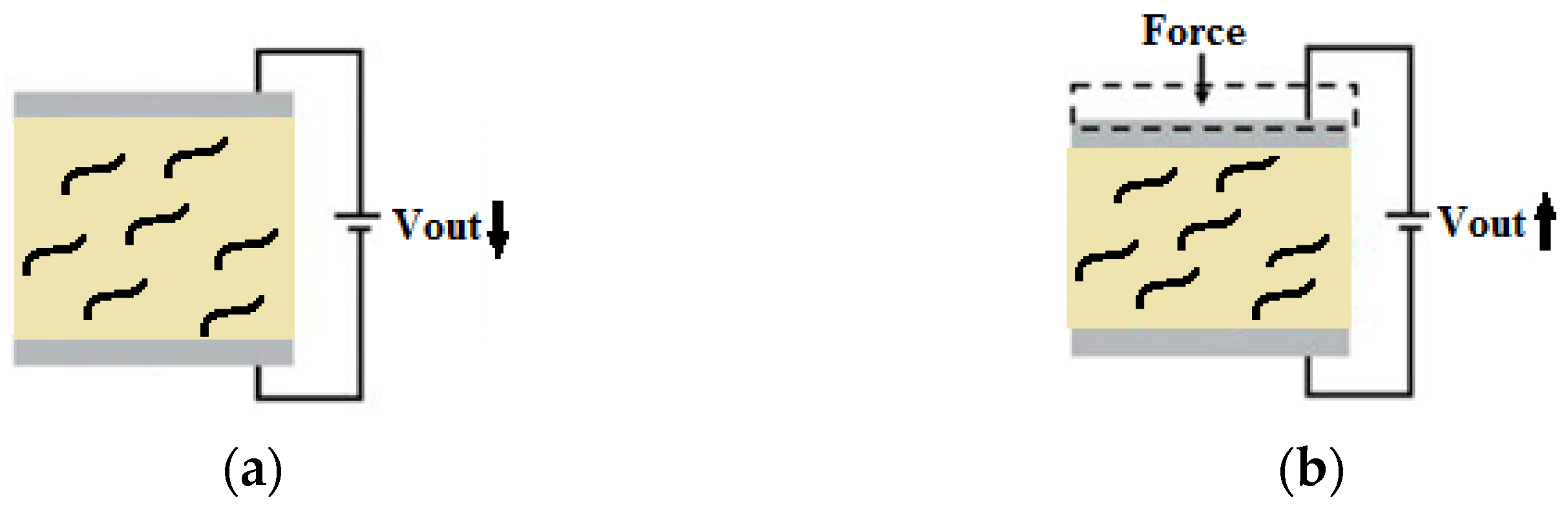
Figure 1a shows an overview of the material at the contact point of the two sensor sheets with voltage bias. The sensor consists of two conductor materials with carbon nanotube material in the middle.
Figure 1b shows a cross-section of the sensor under mechanical pressure, in which the distance between the conductors is shorter, i.e., the impedance of that sensor decreases. Sensors with a sensing area of 32 × 37.5 cm
2 can detect as many as 2288 sensing points with an accuracy distance of 0.5 cm. To read larger areas, it is necessary to combine multiple sensors. As such, we combined 10 sensors to be able to measure the area of a person lying flat.
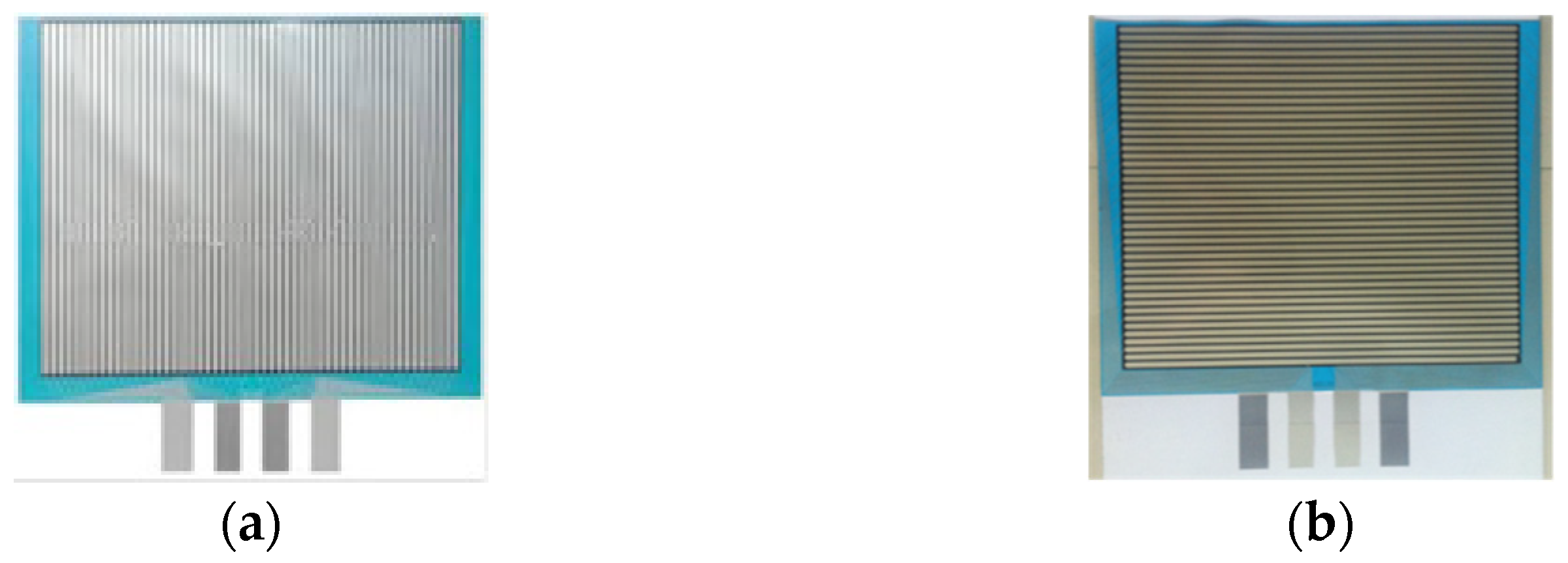
Figure 2 shows photographs of the sensor from the top layer (
Figure 2a) and the bottom (
Figure 2b). The output impedance range of every sensor is between 20 kΩ–20 MΩ, which correlates with a pressure range 0–20 kPa. We get this value by measuring the impedance when the sensor is under no pressure (0 kPa), i.e., its impedance is 20 MΩ. Then, we add pressure by 2 kPa increments until the impedance no longer changes, i.e., when the sensors are under 20 kPa of pressure.
3. Sensor Controller and Communication Design
This system consists of 10 sensors and a 10-sensor controllers. Each controller has one Atmega MCU, a multiplexer, and a demultiplexer. The column of each sensor is designated using a 1 to 64 demultiplexer. After the selection, the voltage value of the sensor is read and converted into a digital value [
16]. The column designation reads all 52 columns, and then the multiplexer value increases to select the next row until all 44 rows have been selected.
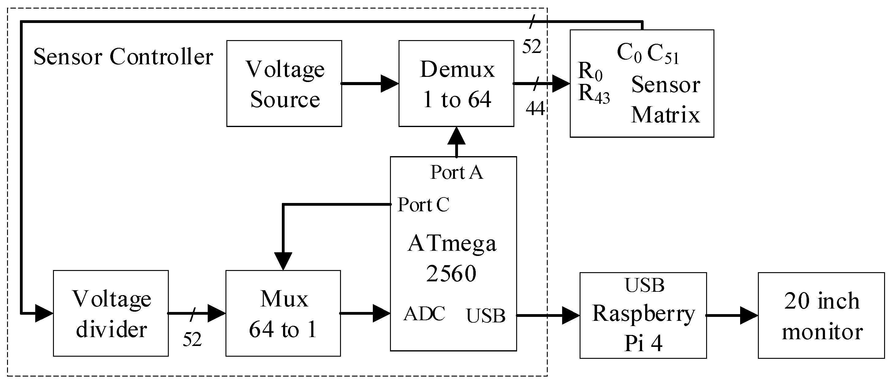
Figure 3 shows a system block diagram for all 52 columns of sensors arranged in 44 rows. Each cross-section is an individual sensor out of a series of sensors in rows or columns, so with 52 columns and 44 rows, we have 52 × 44 sensors, i.e., 2288 sensors.
Since the sensor is piezoresistive, the value read by the system must include resistance. The system (ATMEGA2560 by Atmel, San Jose, CA, USA) reads voltage, so the resistance value must be converted using a voltage divider mechanism with a lower resistor value of 10 kΩ. The voltage conversion into a digital value is performed by the onboard 10-bit analog-to-digital converter of the ATMEGA2560. The digital voltage value (which is the resistance of the piezoresistive sensor) is transferred to the host computer using a serial connection (RS-232) emulation via a USB connection. Ten sheets of sensors are utilized to map a person’s entire body, as described in
Figure 3. When the computer reads the data from each sensor sheet, the ATMEGA2560 sends an ID tag for each sensor embedded on the ATMEGA2560 system. Therefore, the pressure sensor matrix placement will be in the proper place on the pressure display on the monitor.
The host computer receives the data from the ATMEGA2560 when it starts sending data preceded by the sheet identification. The data streams sequentially from row, column one to column two, and so on. The sequence for the second row of sensors is repeated until all rows have been read. The method of data collection for the second to the tenth sheet is the same. After data acquisition, the sensor controllers wait for the computer to finish processing the data; then, the process is repeated.
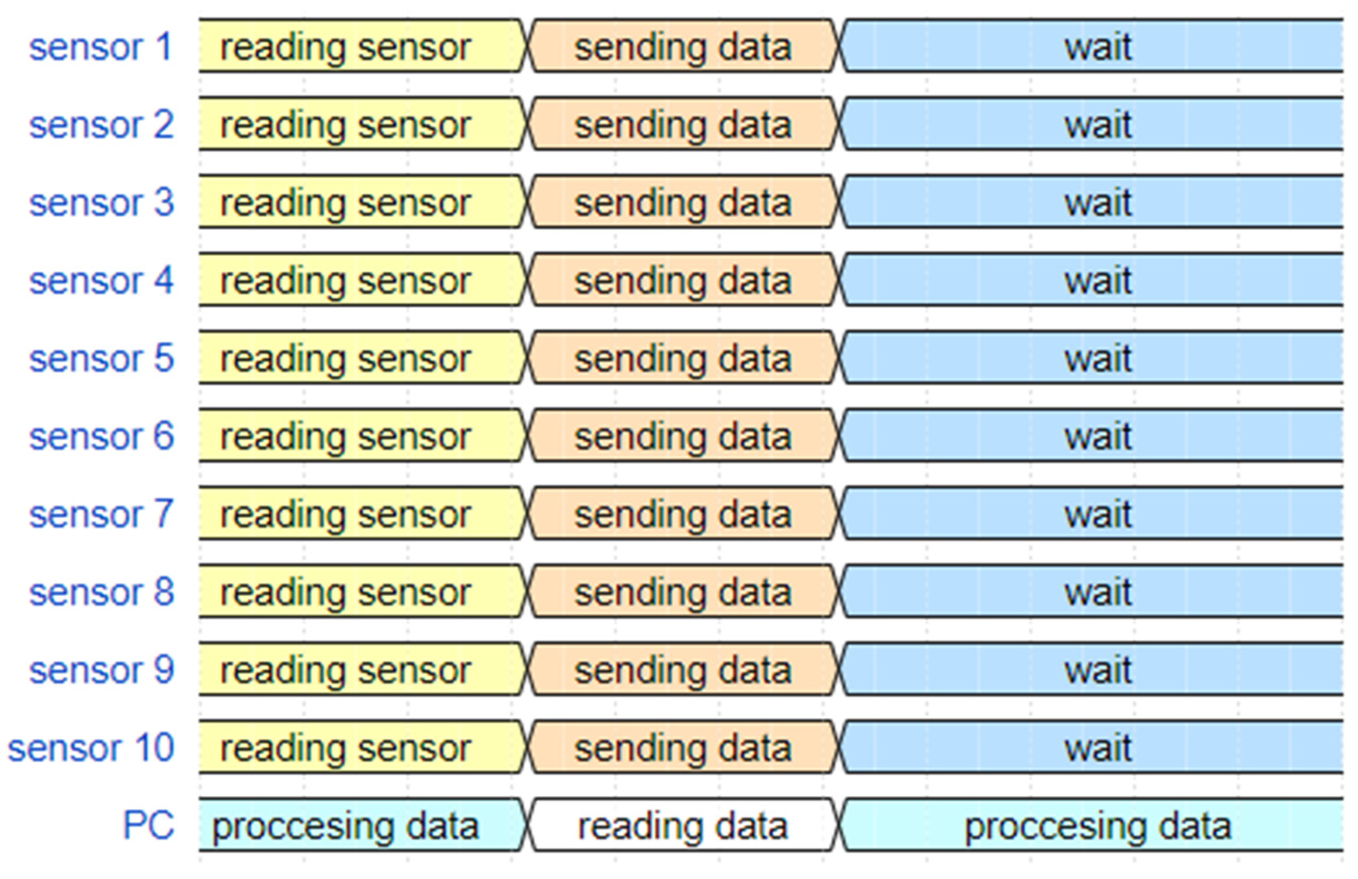
Figure 4 shows a timing diagram of all sensors, together with the host computer, during the data exchange. Every sensor controller reads data from the pressure matrix as described previously, and then sends that data immediately via a serial connection emulator. There are ten virtual connections, and the host computer receives data randomly and processes it according to the ID tag. After sending the data, the sensor controllers wait for the next cycle to start. All ten sensors can start sending data at any time, i.e., whenever the data is ready. When the first data set exchange has finished, the second sensor controller starts sending data, which is not always in order.
4. Calibration and Gain Adjustment
To avoid data drifting, we connected the MCUs to the same Vcc reference parallel and check the output after input voltage conversion at 1V, 2V, 3V and 4V. When reading the same voltage, the digital value was same, indicating that the ADC was synced.
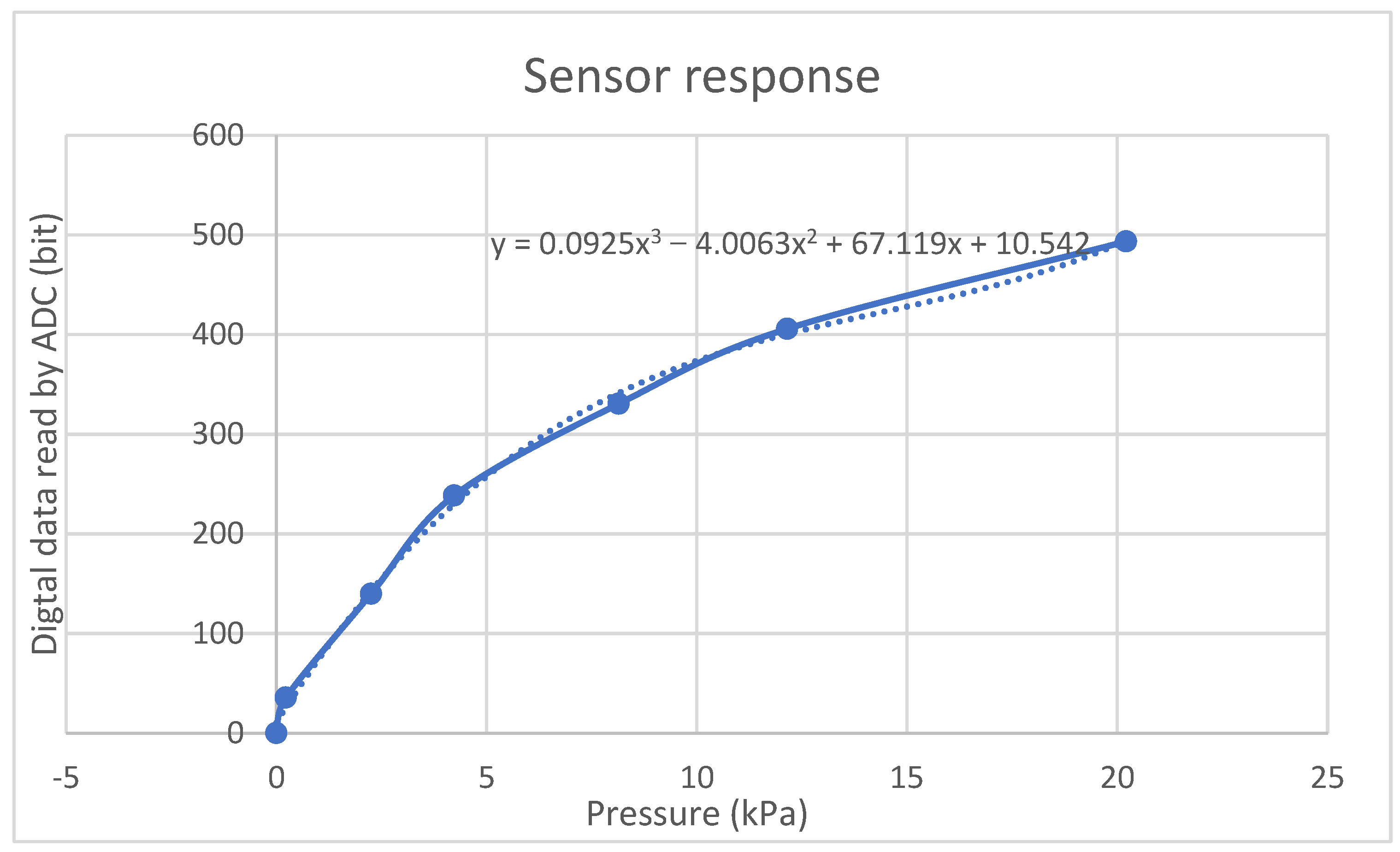
To determine the sensor output characteristics, we applied a pressure of 0.2 kPa, 2 kPa, 4 kPa, 8 kPa, 12 kPa, and 20 kPa to the sensors.
Figure 5 shows the output characteristic of the pressure sensor. From the output characteristics, we can then get the equation. When measuring the sensors one by one, each one has a slight difference in terms of its output because of a minor difference in sensor thickness; as such, the gain needs to be adjusted. Every point of the piezoresistive sensor varies within the sheet. Therefore, it is necessary to calibrate each sensor to obtain a consistent weight value. Sensors were calibrated using a 500 g weight. The gain and offset were then calculated using standard span and zero adjustments. The sensor output characteristic gradually decreased in value as it approached the maximum pressure.
This gain adjustment was performed by multiplying the resistance with a 500 g weight so that when the same load was applied to each sensor, the pressure value would be the same.
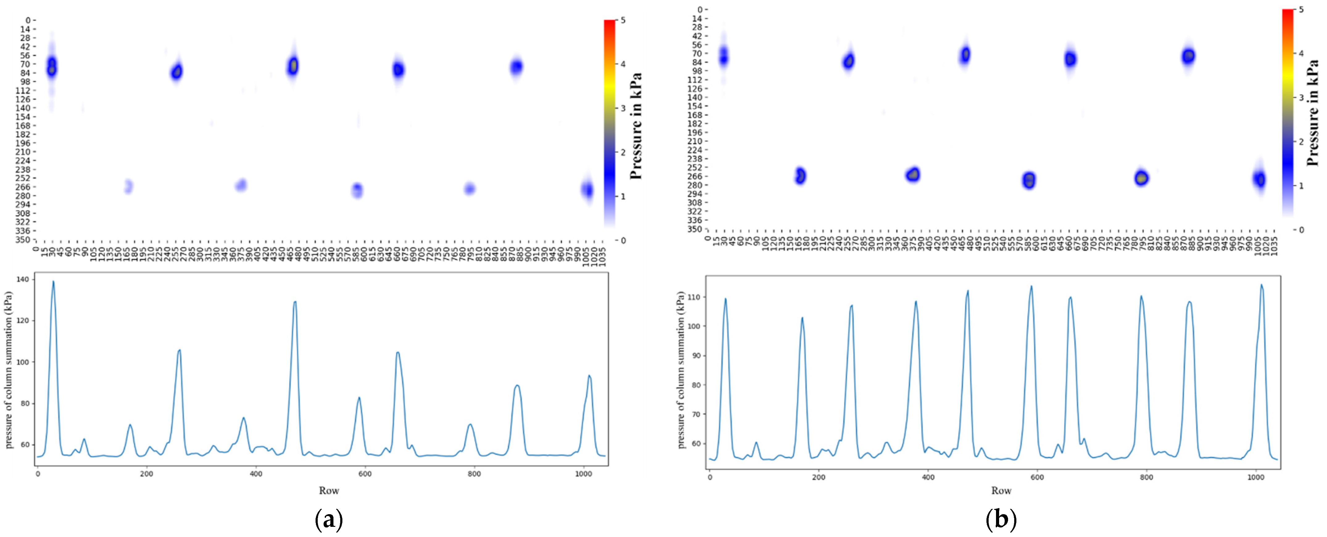
Figure 6a shows a poor quality of the 10-point heatmap before the calibration process.
Figure 6b shows the same points after calibration with the same heatmap display, and which demonstrates improved consistency. The numerical values of the data after calibration also show consistency, as displayed at the bottom of the picture.
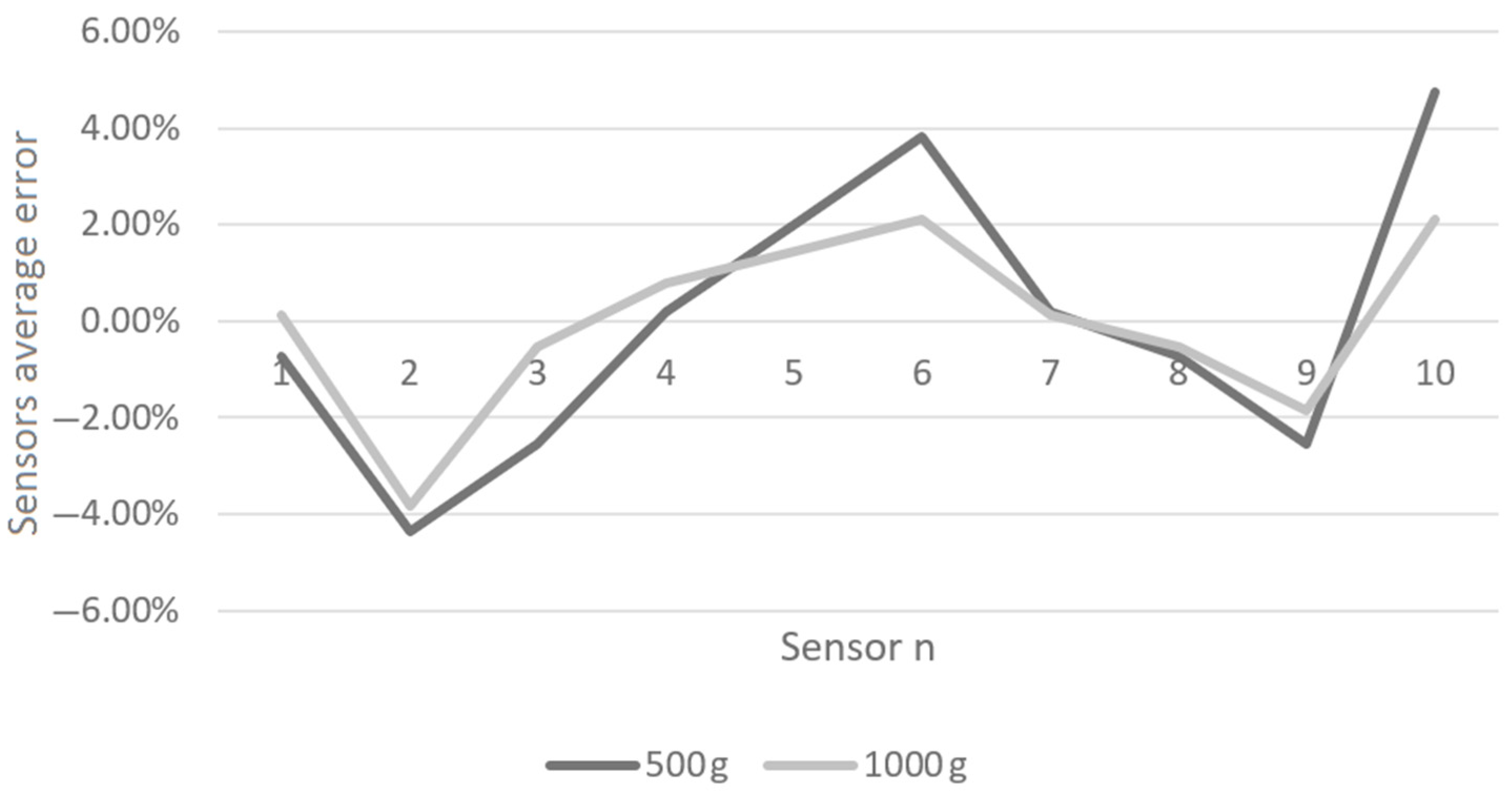
We undertook a trial test with a 1000 g load to show the effectiveness of the calibration process. Ten adjacent sensors were tested with the same load.
Figure 7 shows the outputs of the ten sensors measuring the 500 g and 1000 g weight. As shown, the maximum deviation was 4%, as indicated by Sensor 2. Other sensors showed a variation of less than 2%, as indicated by the light gray line. The dark gray line shows the deviation, i.e., about 4%, when the piezoresistive sensors measured a 500 g weight.
5. Combining and Processing Data
Ten-sensor sheets were tiled together into a combination of two sensors in width and five in height to cover the entire surface. The sensor sheet controller ID indicates the proper position of the sensor sheet relative to the human body. Since the position and the orientation of the sensor sheets are known beforehand, the host computer will arrange the final position of the sensor matrix according to the position of the sensor sheets.
Data acquisition from the ten-sensor sheets started from the patient’s right side from the top sheet (i.e., the position of the subject’s head) down to the feet. Similarly, acquisition of the left side started from the head and continued to the feet. Keep in mind that the sensors on the left-hand side had to be flipped because of the connector position; therefore, the left-hand side data had to be adjusted to get the proper pressure image by reading the rows in reverse order.
After data acquisition, the data were arranged into an 88 × 260 matrix. The numeric results of the sensors were converted into a color-coded heatmap using Matplotlib. The next step was to smooth the data to make it look better, and the last step was the convolution to further enhance the data. All the image processes used Keras image data preprocessing to reduce the need for computer processing power.
The heatmap upscaling process involves through several stages. The first is to threshold the data starting from 0.5 kPa, because when sensors are under no pressure, the result indicates 0–0.5 kPa. Inconsistencies could result from spurious noise from the sensor itself and some simple movement of the person laying on the sensor sheets. The second step was Gaussian filtering to reduce high-level noise by averaging neighboring data. The Gaussian filtering process is widely used to smooth data in image processing [
17]. We used a Gaussian filter because distribution was centered around the zero frequency with positive and negative frequencies at both sides. With Keras, the data was easier to investigate.
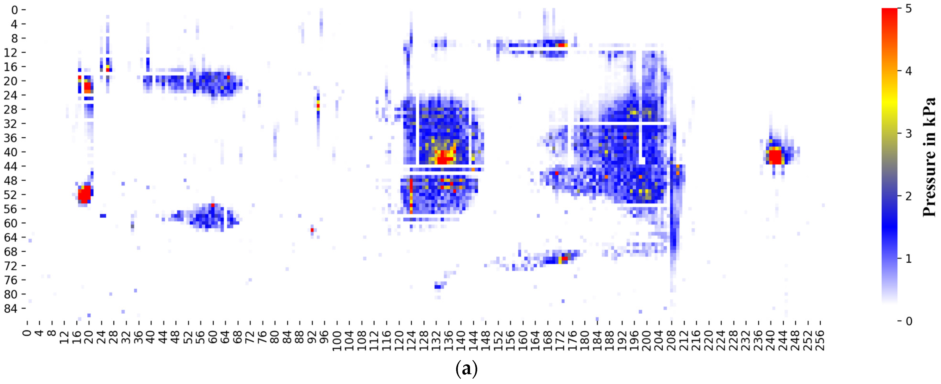
Figure 8a shows the raw image data before processing. In this image, several red areas had high-pressure values and were difficult to differentiate the adjacent values.
Figure 8b shows the image after upscaling and smoothing using Keras and Gaussian filters. This figure shows the smoothing effect markedly, as compared to the previous image.
6. Results and Discussion
The data obtained need to be analyzed to get the character of the data and what results can be concluded. Data from several people were compared to obtain their characteristics, besides data from points that received high pressure, namely the heels, tailbone, shoulders, and head, were compared.
6.1. Comparing Data with a Different Person
Several trial runs involve three subjects to ensure consistency and data reading on the system. The three subjects have weights of 48 kg, 76 kg, and 78 kg, respectively. After data processing, data mapping, and data smoothing, the host computer creates a map of the human body pressure map.
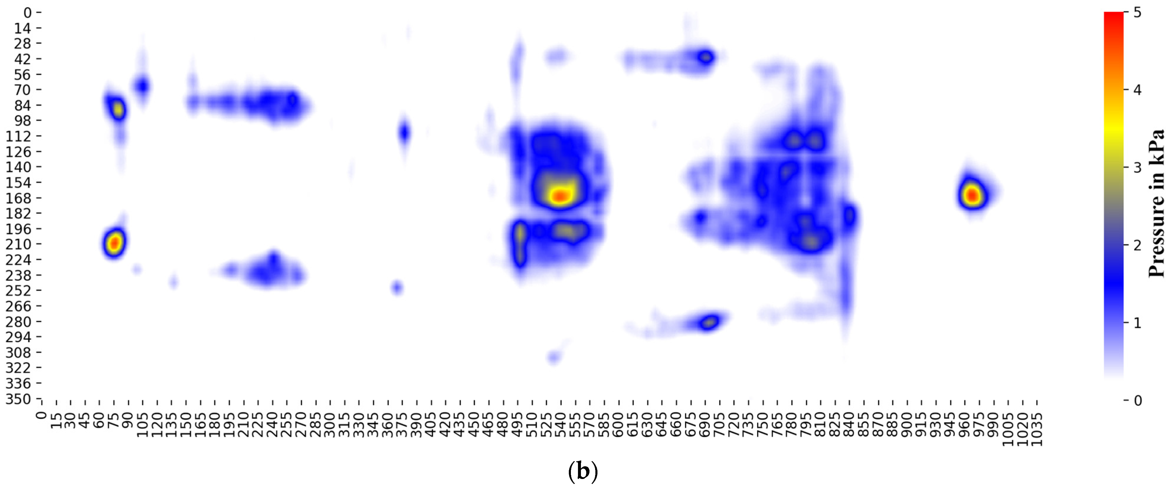
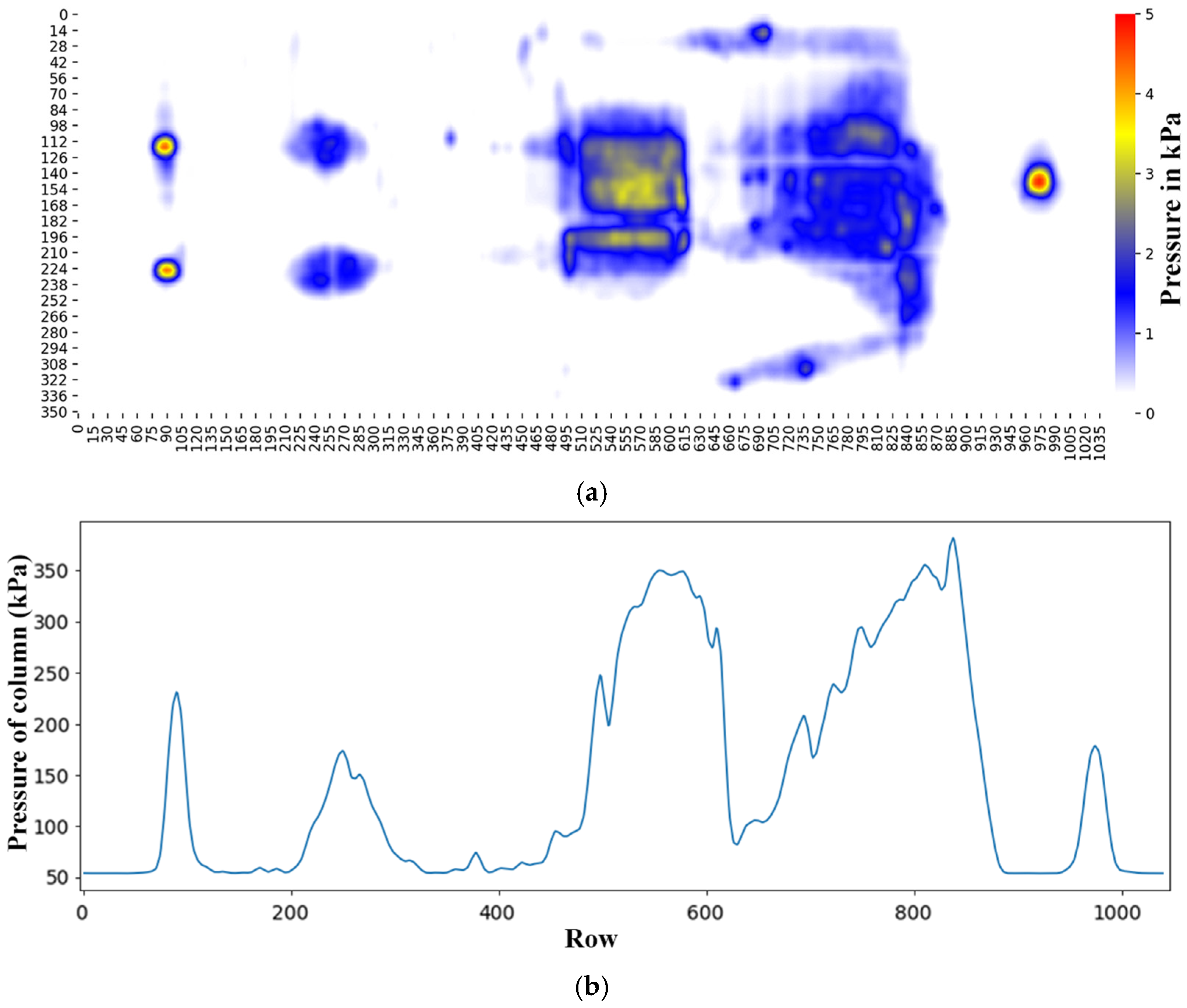
Figure 9 shows the pressure map of a 78 kg person lying on the sensors. The color map of red has the highest pressure, then the yellow color, and the lowest in the blue map.
Figure 9 shows the pressure mapping indicating that the tailbone, shoulders, and head have the highest pressure (red color). The bottom figure shows the sum of pressure for each column, which is the pressure profile of the person’s entire body from the right hand to the left-hand side of the body.
Heatmap presentation of the pressure will only provide the relative pressures among body parts but not the pressure values. There is a numerical evaluation of the pressure complementing the after conducting visual analysis. There are numerical values extracted from the heatmap for the body’s high-pressure region, such as the heel, tailbone, upper back, and head.
Table 1 shows the numerical values of the pressure of such body parts mentioned above.
Table 1 shows the weight increase of the two subjects (48 kg and 76 kg) result in increased pressure of the specific body parts mentioned above. The most significant pressure increase is in the upper back area, which is about 20%. Other body parts also show increased pressure but are not as significant as the upper back. This result is consistent with the two subjects with different measurement occasions. The increased pressure values on the heels, tailbone, and head are only about 8%. This data shows that the most significant pressure increase of a heavier person lying on their back is the upper back area, increasing the risk of decubitus as can be seen in
Figure 9.
Comparing two subjects with similar weights (76 kg and 78 kg) shows negligible pressure increase in the tailbone and upper back area. The difference in value is still within the error range of 3% for the tail bone and upper back area, while the pressure values at the head and heel are the same. These value differences at the tailbone and upper back area might be the slight weight increase of the subject.
Table 1 also shows that there are three subjects tested of different weights and the increased weight increases the pressure on the pressure matrix sensor. Higher weight does not have a linear relationship with the pressure at critical body parts. A weight increase of 50% only provides a 20% pressure increase in the upper back area. Lower increased pressure value could result from distributed weight by the heavier subject. A slight increase in subjects’ weight does not increase the pressure value at the heel and head area. Value in
Table 1 shows pressure summation from the entire coulomb (44 rows) because people who weigh more tend to be larger, which means the pressure is distributed over a larger area.
6.2. Analyzing Pressure from the Selected Pixel/Column
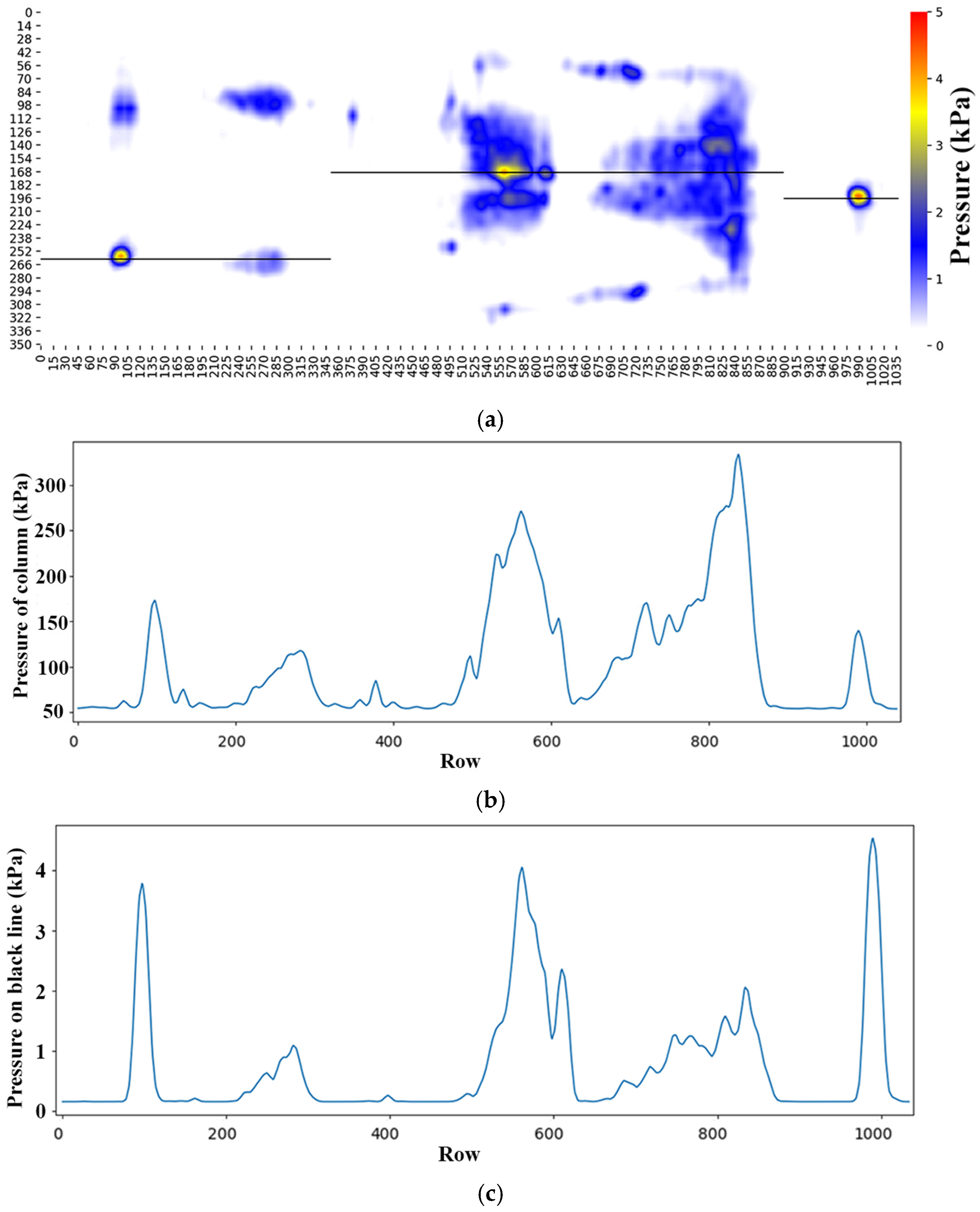
Figure 10 shows a pressure profile of a subject lying down on the top picture. Specific data from this figure are extracted, such as the left heel to the upper part of the left leg, as indicated by the straight black line in the figure. Similar data extraction is conducted from the tail bone to the subject’s head, as indicated by the black line. The bottom figure shows the data plotting from the left heel to the head along the black line described previously. This plot also indicates similar results as the heatmap but with numerical values. This plot clearly shows the peak of the pressure and which part has the highest value.
Figure 10c shows data as in
Figure 10b but for pressure value along the black line. The pressure profile is along the black line shown in the figure. In this figure, the pressure profile indicates that the peak pressure is at the said position mentioned previously. The heatmap diagram for the pressure presentation provides an immediate mark about the highest pressure of the profile for all the subjects. The data numerical data (plotted) also corroborate the finding using the heatmap diagram.
6.3. Warning during Prolonged Skin Exposure to Pressure
Decubitus occurs because there is pressure on one area of the body continuously. To prevent decubitus duration of skin pressing the surface need to be maintained. Duration maintained by monitoring area with pressure more than 2.5 kPa. We choose 2.5 kPa because after observing subject with weight 48 kg and 76 kg area that vulnerable to decubitus like heel, tailbone, back, and head have pressure more than 2.5 kPa. 2.5 kPa chosen because the average pressure of the area under pressure is 2.5 kPa. To find out whether the subject changes position or not, timer used and triggered when the measuring point passes the pressure of 2.5 kPa, and stopped when pressure dropped to below 2.4 kPa more than 10 s.
7. Conclusions
This work shows the pressure profile of a subject lying on a set of pressure matrix sensors. The data collection uses Raspberry Pi 4 Model B with 8 GB memory for data processing and display. Every sensor sheet uses an ATMEGA 2560 as its sensor controller. The pressure profile shows that the highest pressure is in the heels, tail bone, upper back, and head, indicating a high risk of decubitus in these areas. The increased weight of the subject does not increase the pressure linearly. Instead, the pressure near the heel and the head tend to be constant. To prevent decubitus, we need to check whether the pressure point is not moving for a specific time and warn the patient so that preventive measures can be taken. For the next stage, detection of decubitus can be done using artificial intelligence after getting enough data to conduct training.
Author Contributions
Conceptualization, H.P. and A.F.M.; methodology, H.P.; software, A.F.M.; validation, A.F.M., H.P. and L.A.; formal analysis, A.F.M., H.P. and L.A.; investigation, A.F.M., H.P. and L.A.; resources, H.P.; data curation, A.F.M., H.P. and L.A.; writing—original draft preparation, A.F.M.; writing—review and editing, H.P.; visualization, A.F.M.; supervision, H.P.; project administration, H.P. and L.A.; funding acquisition, H.P. All authors have read and agreed to the published version of the manuscript.
Funding
This research was funded by Ministry of Research, Technology and Higher Education under contract number 150L/WM01.5/N/2021.
Institutional Review Board Statement
Not applicable.
Informed Consent Statement
Not applicable.
Data Availability Statement
The data presented in this study are available on request from the corresponding author.
Conflicts of Interest
The authors declare no conflict of interest.
References
- Yin, Z.; Yin, M.J.; Liu, Z.; Zhang, Y.; Zhang, A.P.; Zheng, Q. Solution-Processed Bilayer Dielectrics for Flexible Low-Voltage Organic Field-Effect Transistors in Pressure-Sensing Applications. Adv. Sci. 2018, 5, 1701041. [Google Scholar] [CrossRef] [PubMed] [Green Version]
- Song, Y.; Chen, H.; Su, Z.; Chen, X.; Miao, L.; Zhang, J.; Cheng, X.; Zhang, H. Highly Compressible Integrated Supercapacitor–Piezoresistance-Sensor System with CNT–PDMS Sponge for Health Monitoring. Small 2017, 13, 1702091. [Google Scholar] [CrossRef] [PubMed]
- Yogeswaran, N.; Navaraj, W.T.; Gupta, S.; Liu, F.; Vinciguerra, V.; Lorenzelli, L.; Dahiya, R. Piezoelectric graphene field effect transistor pressure sensors for tactile sensing. In Applied Physics Letters; American Institute of Physics Inc.: College Park, MD, USA, 2018; Volume 113, p. 14102. [Google Scholar] [CrossRef]
- Jun, S.; Han, C.J.; Kim, Y.; Ju, B.K.; Kim, J.W. A pressure-induced bending sensitive capacitor based on an elastomer-free, extremely thin transparent conductor. J. Mater. Chem. A 2017, 5, 3221–3229. [Google Scholar] [CrossRef]
- Pickenbrock, H.; Ludwig, V.U.; Zapf, A. Support pressure distribution for positioning in neutral versus conventional positioning in the prevention of decubitus ulcers: A pilot study in healthy participants. BMC Nurs. 2017, 16, 60. [Google Scholar] [CrossRef] [PubMed]
- Rotaru, G.M.; Pille, D.; Lehmeier, F.K.; Stämpfli, R.; Scheel-Sailer, A.; Rossi, R.M.; Derler, S. Friction between human skin and medical textiles for decubitus prevention. In Tribology International; Elsevier: Amsterdam, The Netherlands, 2013; Volume 65, pp. 91–96. [Google Scholar] [CrossRef]
- Ellis, M. Pressure ulcer prevention in care home settings. Nurs. Older People 2017, 29, 29–37. [Google Scholar] [CrossRef] [PubMed]
- Horton, S.; Sullivan, R.; Flanigan, J.; Fleming, K.A.; Kuti, M.A.; Looi, L.M.; Pai, S.A.; Lawler, M. Delivering modern, high-quality, affordable pathology and laboratory medicine to low-income and middle-income countries: A call to action. Lancet 2018, 391, 1953–1964. [Google Scholar] [CrossRef]
- Turner, H.C.; Van Hao, N.; Yacoub, S.; Hoang, V.M.T.; Clifton, D.A.; Thwaites, G.E.; Dondorp, A.M.; Thwaites, C.L.; Chau, N.V.V. Achieving affordable critical care in low-income and middle-income countries. BMJ Glob. Health 2019, 4, e001675. [Google Scholar] [CrossRef] [PubMed] [Green Version]
- Daniel, H.; Bornstein, S.S.; Kane, G.C. Addressing Social Determinants to Improve Patient Care and Promote Health Equity: An American College of Physicians Position Paper. Ann. Intern. Med. 2018, 168, 577. [Google Scholar] [CrossRef] [PubMed] [Green Version]
- Pranjoto, H.; Sarwono, W.C.; Miyata, A.F.; Agustine, L. Raspberry Pi-based Decubitus Reducing Mattress with Air Pressure Monitoring System and Air Leaks Detector. In Proceedings of the 2021 4th International Conference of Computer and Informatics Engineering (IC2IE), Depok, Indonesia, 14–15 September 2021; pp. 418–423. [Google Scholar] [CrossRef]
- Miyata, A.F.; Agustine, L.; Sitepu, R.; Joewono, A.; Pranjoto, H. Graphical Pressure Mapping of a 2288 Sensing-Point Matrix Pressure Sensor Using Raspberry Pi. In Proceedings of the 2020 2nd International Conference on Broadband Communications, Wireless Sensors and Powering (BCWSP), Yogyakarta, Indonesia, 28–30 September 2020; pp. 26–30. [Google Scholar] [CrossRef]
- Huang, W.; Dai, K.; Zhai, Y.; Liu, H.; Zhan, P.; Gao, J.; Zheng, G.; Liu, C.; Shen, C. Flexible and Lightweight Pressure Sensor Based on Carbon Nanotube/Thermoplastic Polyurethane-Aligned Conductive Foam with Superior Compressibility and Stability. ACS Appl. Mater. Interfaces 2017, 9, 42266–42277. [Google Scholar] [CrossRef] [PubMed]
- Li, X.; Gao, F.; Wang, L.; Chen, S.; Deng, B.; Chen, L.; Lin, C.H.; Yang, W.; Wu, T. Giant piezoresistance in B-doped SiC nanobelts with a gauge factor of-1800. ACS Appl. Mater. Interfaces 2020, 12, 47848–47853. [Google Scholar] [CrossRef] [PubMed]
- Tran, A.; Zhang, X.; Zhu, B. Mechanical Structural Design of a Piezoresistive Pressure Sensor for Low-Pressure Measurement: A Computational Analysis by Increases in the Sensor Sensitivity. Sensors 2018, 18, 2023. [Google Scholar] [CrossRef] [Green Version]
- Li, Q.; Luo, S.; Wang, Q.-M. Piezoresistive thin film pressure sensor based on carbon nanotube-polyimide nanocomposites. Sens. Actuators A Phys. 2019, 295, 336–342. [Google Scholar] [CrossRef]
- Tronarp, F.; Garcia-Fernandez, A.F.; Sarkka, S. Iterative Filtering and Smoothing in Nonlinear and Non-Gaussian Systems Using Conditional Moments. IEEE Signal Process. Lett. 2018, 25, 408–412. [Google Scholar] [CrossRef] [Green Version]
| Publisher’s Note: MDPI stays neutral with regard to jurisdictional claims in published maps and institutional affiliations. |
© 2022 by the authors. Licensee MDPI, Basel, Switzerland. This article is an open access article distributed under the terms and conditions of the Creative Commons Attribution (CC BY) license (https://creativecommons.org/licenses/by/4.0/).


