Estimation of FAVAR Models for Incomplete Data with a Kalman Filter for Factors with Observable Components

Department of Mathematics, Technical University of Munich, 85748 Munich, Germany
*
Author to whom correspondence should be addressed.
Econometrics 2019, 7(3), 31; https://0-doi-org.brum.beds.ac.uk/10.3390/econometrics7030031
Submission received: 9 February 2019
/
Revised: 15 June 2019
/
Accepted: 28 June 2019
/
Published: 15 July 2019
Abstract
:This article extends the Factor-Augmented Vector Autoregression Model (FAVAR) to mixed-frequency and incomplete panel data. Within the scope of a fully parametric two-step approach, the alternating application of two expectation-maximization algorithms jointly estimates model parameters and missing data. In contrast to the existing literature, we do not require observable factor components to be part of the panel data. For this purpose, we modify the Kalman Filter for factors consisting of latent and observed components, which significantly improves the reconstruction of latent factors according to the performed simulation study. To identify model parameters uniquely, the loadings matrix is constrained. In our empirical application, the presented framework analyzes US data for measuring the effects of the monetary policy on the real economy and financial markets. Here, the consequences for the quarterly Gross Domestic Product (GDP) growth rates are of particular importance.
Keywords:
expectation-maximization algorithm; factor-augmented vector autoregression model; forecast error variance decomposition; impulse response function; incomplete data; Kalman FilterJEL Classification:
C33; E44; E521. Introduction
The role of money in the case of monetary policy and its impact on the real ecomony have been thoroughly discussed in the literature. For instance, see Levhari and Patinkin (1968), Grandmont and Younes (1972) as well as Carr and Darby (1981). In this regard, Mankiw (2010, 2014) distinguishes three hypotheses: First, classical dichotomy believes in the neutrality of money, that means, it does not affect the real economy, see for example, Ball and Romer (1990). In this theory, only prices and wages matter. A second group of economists claims that monetary policy may affect the real economy through falling interest rates and raising investments, see for example, Serletis and Koustas (1998). Finally, the current economic theory assumes the neutrality of money in the long run, but it admits the possibility that monetary policy may absorb economic fluctuations in the short run, see for example, Minsky (1993). Hence, monetary policy implications are crucial for central banks and it explains why there is abundant literature about measuring the effects of monetary policy.
Vector Autoregression Models (VARs) have become the standard approach for identifying and measuring the effects of monetary policy innovations on macroeconomic variables since Bernanke and Blinder (1992) and Sims (1992). A main advantage of this method is that it clearly discloses the effects of shocks. Unfortunately, VARs are restricted to a limited number of times series, which may result in a trade-off for empirical applications. On the one hand, a comprehensive model must take into account the full information spectrum used by central banks and external sources. On the other hand, VARs with too many variables cannot uniquely be estimated based on small data samples. Then, a pre-analysis is required to extract the most relevant, sparse data from the full information spectrum. However, if the resulting sparse panel data does not sufficiently reflect the original data, policy shocks are measured with errors and misleading results are obtained. A second drawback is that their Impulse Response Functions (IRFs) merely consider the few included variables covering a small subset of the universe central banks care about. Here, IRFs map how a variable of interest reacts to exogenous shocks over time. The choice of specific time series representing an economic concept like “real activity” is arbitrary to some degree and thus, denotes a third disadvantage of the VAR approach. Bernanke et al. (2005) introduced the Factor-Augmented Vector Autoregression Models (FAVARs) which combine the VAR approach with factor analysis. The main idea behind FAVARs is to extract the information inherent in large panel data by a few factors and some observable variables. Because of this, a FAVAR consists of two equations: The transition equation displays the joint dynamics of the observed and latent factors as a VAR process, while the measurement equation shows the relation between both factors and some additional panel data.
For estimating FAVARs several procedures can be pursued. For instance, Bernanke et al. (2005) suggested a non-parametric two-step approach using Principal Component Analysis (PCA) and Ordinary Least Squares Regression (OLS). Additionally, they derived a single-step Markov Chain Monte Carlo method. Bork (2009) as well as Bańbura and Modugno (2014) applied Expectation-Maximization Algorithms (EMs) instead. Sometimes, the estimation of FAVARs relies on complete panel data, whose updating frequency is either monthly (Bernanke et al. 2005; Bork 2009; Wu and Xia 2014) or quarterly (Ellis et al. 2014). In case of macroeconomic data, the Unemployment Rate and Consumer Price Index are monthly published, but the Gross Domestic Product (GDP) is quarterly reported. All three indices rank among the relevant guides for monetary policy, although they are not ready at the same frequency. Therefore, the question of how to best profit from such data arises. A simple solution takes the least frequently updated time horizon, for example, the quarterly one. However, this approach ignores all monthly information.
By contrast, we incorporate well-known results regarding temporal aggregation and missing observations to obtain balanced panel data (Stock and Watson 1999, 2002b; Mariano and Murasawa 2003, 2010; Bańbura et al. 2011, 2013). Thereby, we introduce for each observed time series an artificial, complete analog and define a proper relation between both. Depending on the relation type, we distinguish between stock, flow and change in flow variables. In the past, among others, Schumacher and Breitung (2008); Stock and Watson (2002b) and Bańbura and Modugno (2014) tackled data irregularities in the area of factor models, while Bańbura and Modugno (2014); Boivin et al. (2010); Bork (2015) and Marcellino and Sivec (2016) did the same for FAVARs.
In the presence of data incompleteness, Kalman filtering methods and EMs enable Maximum-Likelihood Estimation (MLE). With regard to this, the seminal work of Dempster et al. (1977) showed how to integrate missing data out of the likelihood function. Shumway and Stoffer (1982) deployed EMs for time series with missing observations. At the same time, Rubin and Thayer (1982) and Watson and Engle (1983) estimated factor models using EMs. Theoretical aspects of EMs, in particular, some convergence properties were discussed in Wu (1983). Finally, Bańbura and Modugno (2014) developed an EM for estimating dynamic approximate factor models with arbitrary patterns of missing data. Bańbura and Modugno (2014) as well as Bork (2015) admit time-dependent selection matrices to exclude missing data from their MLE. Their state-space representations already take into account which data type1 each variable belongs to and so, they have a single EM instead of two. However, they must adjust the whole state-space representation, as soon as for example, new time series are added or old ones are removed. By contrast, our two-step approach requires changes of single equations for balanced data instead of the overall model formulation which bears less risks and so, denotes another advantage of our procedure. The non-parametric method in Boivin et al. (2010) coincides with ours, if our second EM is replaced by the two-step principal component approach of Bernanke et al. (2005). In general, this second EM coincides with Bork (2009), Bork et al. (2010) and Bańbura and Modugno (2014). The first EM was introduced in Stock and Watson (1999, 2002b) and was reused in Schumacher and Breitung (2008).
In this paper, we extend the FAVAR of Bernanke et al. (2005) to ragged panel data and make the following three contributions to the existing literature: First, two EMs estimate the model parameters and reconstruct missing obersations in the form of an iterative scheme. The first EM controls the relation between the observed and artificial time series, when it constructs balanced data. Based on this, the second EM performs the actual MLE. Our second contribution is that the observable factors of the FAVAR are not needed to be a part of the panel data as in Bork (2009) and Marcellino and Sivec (2016). Therefore, the loadings matrix can be constrained without resorting the panel data. This is convenient for model selection since existing estimation methods require a special variable order in the panel data. Nevertheless, for comparison reasons of our empirical results we perform the same data pre-processing as Bork (2009) including the distinction between slow- and fast-moving variables as proposed in Bernanke et al. (2005). Finally, our last contribution is the adaption of the classical Kalman Filter (KF) for the observable factor components. In this regard, we derive KF equations for a refined state-space representation and show the superiority of our modified KF estimation in a simulation study.
In the empirical study, we investigate the effects of the United States (US) monetary policy on its real economy. Thereby, we use data similar to Bernanke et al. (2005). In addition, we have quarterly indices, for example, GDP, discontinued data, for example, Deutsche Mark-US Dollar Foreign Exchange (FX) and later starting variables, for example, Euro-US Dollar FX. The updating frequency is monthly. The time period ranges from January 1959 until October 2015 covering several crises. We evaluate the impact of the monetary policy decisions using Impulse Response Functions (IRFs) and Forecast Error Variance Decompositions (FEVDs). The confidence intervals of the IRFs arise from a non-parametric bootstrap method.
The remainder of this paper is structured as follows: In Section 2, we discuss the definition of FAVARs and derive an alternative estimation method for incomplete panel data. Thereby, we derive estimates for missing observations. In Section 3, we compare the estimation quality of the suggested estimation method with already existing ones. In Section 4, we measure the impact of the US monetary policy on the real economy based on mixed-frequency US panel data. In Section 5, we summarize our findings and outline directions for the future research. The appendices provide detailed algorithms, results of the Monte Carlo (MC) simulations, data descriptions and illustrations of the empirical study.
2. Mathematical Background
We start with the definition of FAVARs and show that parameter ambiguity may affect the covariance matrices of idiosyncratic shocks. At this stage, we include identification conditions from Bai et al. (2015). In a next step, we modify the KF from Bork (2009) to take into account that factors are partially observable. Incomplete time series are reconstructed using the EM of Stock and Watson (1999, 2002b).
2.1. Parameter Ambiguity and Identification Restrictions
Usually, VARs accomodate a limited number of time series.2 In this regard, FAVARs are more indulgent and support the modeling of high-dimensional data. Similar to Dynamic Factor Models (DFMs), FAVARs comprise a transition equation and a measurement equation. But there is an important difference between both. The transition equation of DFMs describes the dynamics of latent factors at time t, whereas the one of FAVARs maps the joint dynamics of latent factors and observable variables . This is why the joint factors are partially observable.
In the scope of monetary policy analysis with FAVARs, often covers measures controlled by central banks such as the US Effective Federal Funds Rate (FEDFUNDS). By contrast, VARs require to collect all data due to . Thus, VARs must balance covering of relevant information and data dimension. In FAVARs, important information, which is not yet part of , is condensed in the latent factors . With this in mind, the transition equation of a FAVAR is given by the following dynamics:
where is a conformable lag polynomial of finite order with and denoting a -dimensional matrix of autoregressive coefficients for . The error vector is supposed to be Gaussian identically and independently distributed (iid) with zero mean and covariance matrix . For simplicity reasons, let each univariate times series part of be standardized with zero mean and standard deviation of one. Furthermore, we assume the VAR process in (1) as covariance-stationary (Hamilton 1994, Proposition 10.1, p. 259).
Equation (1) is a VAR in the variables , if all terms of covering the impact of on are zero (Bernanke et al. 2005). Otherwise, Bernanke et al. (2005) call (1) the transition equation a FAVAR. Moreover, they note: First, the FAVAR in (1) nests a VAR supporting comparisons with general VAR results and the assessment of the marginal contribution of the factors . Second, if the true system is a FAVAR, ignoring the factors and sticking to the simple VAR in will cause biased estimation results and so, the interpretation of IRFs and FEVDs may be faulty.
Next, the hidden factors are obtained from the FAVAR measurement equation. For this purpose, the vector gathers all panel data at time t, where N is “large” (in particular, N may be greater than the sample length T) and holds. As for , let each times series in be standardized. Then, the measurement equation relates the panel data and the partially observed factors as follows:
where and denote loadings matrices of dimension and , respectively. The idiosyncratic error is Gaussian iid with zero mean and covariance matrix . Note, we attach a greater importance to cross-sectional instead of serial error correlation in this article. In this manner, we enter a direction different to the work of Bańbura and Modugno (2014).3 Because of (2), the vector drives the dynamics of . This is why Bernanke et al. (2005) regard all as “noisy measures of the underlying unobserved factors ”. In total, FAVARs are defined by (1) and (2).
The model (1) and (2) is econometrically unidentified, therefore, its parameters cannot be uniquely estimated. For any non-singular matrix R of dimension the measurement equation obeys:
with as the inverse of matrix R. The observability of imposes constraints on the shape of R and so, removes degrees of freedom (Bai et al. 2015). Consequently, the invertible matrix R consists of the following submatrices:
with as zero matrix (Bai et al. 2015, Proposition 2.1). Let be the covariance matrix of the transformed errors from (1), which is given as follows:
Let the invertible matrix be the Schur complement of the upper left block matrix of the matrix . To remove the remaining degrees of freedom inherent in the submatrices and , we consider the special version of the general matrix R defined as follows:
Then, we obtain for vector the identification restrictions IRb from Bai et al. (2015). Thus, the FAVAR in (1) and (2) also meets the following representation:
Note, by construction the equality in (5) is justified (Ramsauer 2017, p. 127). The previous transformation by matrix H decreased the degrees of freedom to . That is, for any rotation matrix with matrix defined by
the FAVAR in (4) and (5) is equivalently rewritten for vector . So, linear constraints on the loadings matrix ensure parameter uniqueness. In this regard, the iterative application of Givens Rotations (Golub and Van Loan 1996, p. 215, Section 5.1.8) enables us to eliminate all remaining degrees of freedom and preserve the shape of matrix G in (6). In total, this theoretically justifies the existence and uniqueness of the FAVAR state-space representation (4) and (5). For more details we refer to Ramsauer (2017). Eventually, for the FAVAR in (4) and (5) with , as lower triangular matrix and diagonal covariance matrix , Bai et al. (2015) provide the asymptotic distribution of the IRFs. As we consider cross-sectionally correlated errors, we pursue the classical approach for IRFs.
2.2. Estimation and Model Selection for Complete Panel Data
For complete panel data, a MLE of the FAVAR (4) and (5) with linear loadings constraints can be done similarly to Dempster et al. (1977), Rubin and Thayer (1982), Shumway and Stoffer (1982) and Bork (2009). Denoting , and , the log-likelihood function of the FAVAR (4) and (5) is . Latent factors are integrated out to obtain the expectation of conditioned on the observations X and Y (the expectation step of EM). An estimation of model parameters ![Econometrics 07 00031 i001]() with
with ![Econometrics 07 00031 i002]() is then obtained by maximizing the expected log-likelihood
under linear loadings constraints (the maximization step of EM). Here, denotes the natural logarithm and is the matrix trace. The conditional moments of the factor are computed using Kalman Filter and Kalman Smoother (KS). By iterating the expectation and maximization steps until convergence of the expected log-likelihood , the EM estimates the model parameters .
is then obtained by maximizing the expected log-likelihood
under linear loadings constraints (the maximization step of EM). Here, denotes the natural logarithm and is the matrix trace. The conditional moments of the factor are computed using Kalman Filter and Kalman Smoother (KS). By iterating the expectation and maximization steps until convergence of the expected log-likelihood , the EM estimates the model parameters .
 with
with  is then obtained by maximizing the expected log-likelihood
The estimation of the FAVAR (4) and (5) with loadings constraints requires knowledge of the factor dimension K and the lag order p. In empirical analyses, both must be specified. For this purpose, we choose the usual Akaike Information Criterion (AIC) and leave more advanced approaches for model selection for the future research. Let and be upper limits of the autoregressive order and factor dimension, respectively, to be tested. Moreover, let be the estimated model parameters for dimensions . Then, we take the pair satisfying:
2.3. Kalman Filter and Smoother
Usually, DFMs with factor dynamics of order are converted into large-dimensional DFMs of order . For FAVAR (4) and (5) and state vector , we receive
![Econometrics 07 00031 i003]()

Bork (2009) as well as Marcellino and Sivec (2016) considered FAVARs as DFMs and made two adjustments. First, they added the observable variables part of to the panel data . Second, they chose the shape of the loadings matrix in (10) such that in was identically mapped to in . In other words, they treated the overall factors as hidden and forced their last M entries to coincide with part of .
By contrast, we use an alternative state-space representation. Namely, we separate latent and observed factors from each other, before the stacking takes place. For vectors and , we reformulate the original FAVAR as follows:
where the shocks are iid Gaussian with zero mean and covariance matrix defined by:
A comparison of the transition Equations (11) and (14) shows that (14) explicitly acknowledges that the factors are partially observed. This enables a modification of the standard KF for observable factor components which, to the best of our knowledge, was not addressed in recent research. Second, we are able to linearly constrain the transition coefficients ![Econometrics 07 00031 i002]() instead of the loadings matrix .5 As usual for KF, we assume known model parameters in (13)–(15) and define the filtration: , for collecting all observations up to time . Then, covers the overall sample . For the hidden factor moments, we set: , and . Analogously, we shorten means and covariance matrices of and , respectively, conditioned on . Algorithm A1 summarizes the adapted KF with factor estimates obtained by PCA as starting values. Note, the KS is not influenced by the observed factor components as shown in Ramsauer (2017).
instead of the loadings matrix .5 As usual for KF, we assume known model parameters in (13)–(15) and define the filtration: , for collecting all observations up to time . Then, covers the overall sample . For the hidden factor moments, we set: , and . Analogously, we shorten means and covariance matrices of and , respectively, conditioned on . Algorithm A1 summarizes the adapted KF with factor estimates obtained by PCA as starting values. Note, the KS is not influenced by the observed factor components as shown in Ramsauer (2017).
instead of the loadings matrix .5 As usual for KF, we assume known model parameters in (13)–(15) and define the filtration: , for collecting all observations up to time . Then, covers the overall sample . For the hidden factor moments, we set: , and . Analogously, we shorten means and covariance matrices of and , respectively, conditioned on . Algorithm A1 summarizes the adapted KF with factor estimates obtained by PCA as starting values. Note, the KS is not influenced by the observed factor components as shown in Ramsauer (2017).2.4. EM-Algorithm for Incomplete Panel Data
Regarding incomplete data we pursue the method of Stock and Watson (1999, 2002b) which introduces for each observed time series an artificial, high-frequency analog and defines a proper relation between both. As in Section 2.2, let N and T denote the number of times series and the total sample length, respectively. The index covers each point in time when new information arrives and thus, captures the highest frequency. For the vector with collects all observations of signal i and the vector serves as its artificial, high-frequency counterpart. Then, we receive:
with . For any complete time series, it holds: and . If a time series is less often updated or there are missing elements, we have: . Furthermore, the shape of the matrix specifies the nature of the relation in (16). In the literature, see for example, Bańbura et al. (2013, ECB working paper), there is a common distinction between stock, flow and change in flow variables6. Sometimes, this classification is discussed as temporal aggregation. The structure of the matrix does not affect our subsequent considerations, this is why we proceed with the general version (16).
Let the matrices , and collect all factors, standardized observations and errors in (4), respectively. The panel data in (4) is supposed to consist of standardized time series, thus, we set: for each time series i with mean and variance . In Section 4, we replace both by their empirical estimates. Here, the vector consists of ones only. Using (4) and (16), we derive for :
where and denote the i-th row of and or the i-th column of E. Following Stock and Watson (1999, 2002b), is reconstructed by its conditional expectation given by
Algorithm A2 summarizes the estimation of FAVARs with incomplete data. Besides the initialization, it consists of an inner and outer EM. The initialization calls for three steps: First, we construct an initial guess for the high-frequency panel data using the given observations. If necessary, gaps are filled by random numbers, interpolation and so forth. At this stage, the time series are not required to obey (16), since this will be automatically achieved by (17). The second step applies the two-step principal component approach of Bernanke et al. (2005) to the standardized panel data . Finally, the third step updates the high-frequency panel data based on the estimated model parameters and observed time series.
The algorithm from Algorithm A2 also tackles the model selection problem. The optimal lag length and factor dimension may change during the estimation procedure. To avoid that changes in affect its termination, changes in the expected log-likelihood instead of the model parameters serve as termination criteria. In this context, we consider relative instead of absolute changes.
3. Monte Carlo Simulation
In the scope of a MC simulation study, we compare the estimation accuracy of our two-step estimation method using the modified KF from Section 2 and three alternative approaches. Besides a non-parametric ansatz based on PCA and OLS, we test two parametric estimation methods treating FAVARs as Approximate Dynamic Factor Models. For all procedures, an outer EM reconstructs complete panel data from observations and latest parameter estimates. Thus, we concentrate on the estimation quality of the modified KF but also address the issue of incomplete panel data.
The underlying data is simulated as follows: For with , let denote the uniform distribution on the interval , while is a diagonal matrix with elements . Furthermore, let and represent arbitrary orthonormal matrices for fixed dimensions . Then, the subsequent FAVARs parameters arise:
Hence, the parameters in (18) specify a general FAVAR instead of its rotated simplification. If all matrices do not satisfy the covariance-stationarity of the factor process , they are redrawn. To prevent us from matrices , whose eigenvalues are close to zero, their eigenvalues are taken from the range of , where the division by i reduces the impact of lagged factors. The restriction to matrices with positive eigenvalues and the division by i are made for simplicity only. Based on (1), we construct the factor sample , standardize all univariate time series in and adjust the matrices and accordingly. Next, we simulate the panel data based on (2) and matrices W and of full column rank. Eventually, we standardize all univariate time series in X and adapt the matrices W and correspondingly.
At this stage, we have complete panel data X. For as target ratio of gaps, we randomly delete elements from each times series serving as stock variable. For flow or change in flow variables, we aggegrate the given data accordingly (for more details see Ramsauer (2017)) such that we receive a regular pattern with observations at times with and . None of the four methods estimates hidden factors for points in time without any observation. Therefore, we reapply this procedure, if the resulting incomplete panel data comprises an empty row.
In the sequel, we focus on the hidden factors F, since the variables Y are observed in full. This is why, we determine for each of the four estimation methods the trace defined as follows:
The trace evaluates the quality of the estimated factors. Since its introduction by Stock and Watson (2002a), it became a common standard in the literature, see for example, Doz et al. (2012) and Bańbura and Modugno (2014). If the hidden factors are perfectly estimated, the trace takes value 1. Otherwise, it is smaller than 1.
For the four estimation methods, Table A1, Table A2, Table A3 and Table A4 report the average of the trace based on 500 MC samples. We focus on the hidden factors, since the variables are observed in full and therefore, do not call for estimation. In Table A1, we estimate the simulated FAVARs with the non-parametric method of Boivin and Giannoni (2008) and Boivin et al. (2010). In Table A2 and Table A3, the EM of Bork (2009) serves as inner EM for the estimation of the model parameters. In Table A2, data reconstruction part of the outer EM (17) relies on filtered instead of observed factors . By contrast, Table A3 directly utilizes observed factors . Finally, Table A4 illustrates the average for our new KF approach. Except for the approach in Table A2, the outer EM in all other estimation methods take the observed vectors into account.
All updates in Algorithm A2 stop, as soon as the absolute value of the relative change in the expected log-likelihood function is below . In particular, the termination criterion controls the data reconstruction (outer EM). Based on the reconstructed data, the criterion terminates the parameter estimation (inner EM). For instance, Bańbura and Modugno (2014, working paper, 2010), employ as termination criterion. In our case, decreasing the termination criterion from to did not significantly improve the estimation quality of our method, but it rather boosted its run time. For all estimation methods we initialize the first guess of the complete panel data in the same way. That is, for each univariate time series, we fill its gaps by the empirical mean of its observations. Finally, we do not address the selection of K and p here.
A comparison of Table A1, Table A2, Table A3 and Table A4 shows: First, irrespective of the estimation method, there are no obvious differences between the trace means of the three data types. Second, a higher percentage of data gaps, ceteris paribus, deteriorates the trace means. Third, longer samples, that is, larger T, improve the trace means. The same holds for panel data covering more variables, that is, larger N. Fourth, higher lag orders improve the trace means, which is rather surprising. So far, all findings are in place for all four estimation methods.
However, some differences exist: First, the estimation methods in Table A1, Table A2 and Table A3 require a work-around to take the observability of into account. For instance, the non-parametric approach repeatedly applies PCA and OLS for separating the impacts of and on from each other. In this regard, the dimensions of the vectors and matter. With a view to Table A1, Table A2 and Table A3, the pairs and have smaller trace means than the pair . By contrast, the estimation method with our modified KF in Table A4 offers for larger trace means than for .
The trace means in Table A4 are usually better than their counterparts in Table A1, Table A2 and Table A3. For clarity, Table A5, Table A6 and Table A7 display the corresponding ratios of trace means from Table A1, Table A2, Table A3 and Table A4, respectively. Thereby, ratios larger than one confirm that the estimation method based on our modified KF outperforms the respective alternative. Note that all ratios in Table A5, Table A6 and Table A7 are larger than one but for the previously mentioned pairs and they exceed one by far. This clearly highlights, why it makes sense to take into account that the variables represent observed factors.
4. Empirical Application
The US economy ranks among the biggest and most important in the world. Moreover, after many years of declining interest rates, in December 2015 the US Federal Reserve decided to raise the Effective Federal Funds Rate (FEDFUNDS) by 25 basis points (bps). So, it was the first large central bank to leave the path of an extremely relaxed monetary policy. Due to this and, of course, for comparisons with Bernanke et al. (2005), Bork (2009, 2015) and Bork et al. (2010), we deal with the impact of the US monetary policy on its real economy in the sequel. At the beginning, we describe the underlying panel data and observable factors. Then, we briefly summarize some technicalities. Eventually, we discuss the estimated Impulse Response Functions and Forecast Error Variance Decomposition.
The underlying panel data is an update of the one in Bernanke et al. (2005), except for 24 variables, which were not available anymore. This is why we have 96 of the original 120 time series over the period from January 1959 until October 2015. Besides the 96 monthly time series, we have 15 partially incomplete time series. Among other things, we are interested in how monetary policy decisions may affect quarterly indices. For this purpose, the quarterly growth rates of GDP, Governmental Total Expenditures, Real Exports of Goods and Services as well as Real Imports of Goods and Services belong to these 15 new time series.7
Monetary policy actions can significantly move Foreign Exchange (FX), especially, if unexpected by markets. As the European Union trades a lot with the US, our data comprises the USD-EUR FX starting in January 1999 and USD FX against the German Mark, French Franc and Italian Lire serving as an approximation for the USD-EUR FX before January 1999. By this means, our data is ragged. Finally, 4 of the 15 new time series offer information about the Federal Reserve Banks’ balance sheets, which have dramatically increased since the financial crisis in 2007/2008. In total, we have 111 macroeconomic indicators for diverse areas of the US economy from January 1959 until October 2015. For a detailed overview including sources, data preprocessing and the distinction between slow- and fast-moving ones based on Bernanke et al. (2005) see Appendix C.
The “Quantitative Easing” programs QE1–QE3 were the response of the Federal Reserve to the problems arising from the financial crisis, after stimulating the economy by lowering the Effective Federal Funds Rate reached its limits in December 2008. For instance, the Federal Reserve massively bought Treasuries and mortgage-backed securities. To obtain a comprehensive picture of the monetary policy actions, the observable factor consists of Currency in Circulation (CURRCIR), St. Louis Adjusted Monetary Base (AMBSL) and Effective Federal Funds Rate (FEDFUNDS). Our estimation method for FAVARs requires the time series to be complete. Therefore, holdings of Treasuries and mortgage-backed securities, which were only available for the years from 2002 until 2015, belong to the panel data.
In Section 3, we aimed at demonstrating the advantages of our updated KF compared to the standard approach. For comparisons of our empirical results to Bork (2009), we now perform the same data pre-processing as originally proposed by Bernanke et al. (2005). In particular, we also distinguish between slow- and fast-moving variables. As soon as the sorting of complete, slow-moving variables has been finished, we repeat this procedure for complete, fast-moving ones, before we add all ragged time series in arbitrary order. Our technical settings are: and . Thus, the termination criteria are not too strict and the run time of the algorithm in Algorithm A2 remains reasonable. An AIC-based model selection (Ramsauer 2017) yields: . In this way, we have larger factor dimensions K and M but a smaller lag order than Bork (2009). Because of this, Table 1 compares the first nine variables of our sorted panel data with their counterparts in Bork (2009). Thereby, we keep the long expressions of Bork (2009) in the second column and apply our abbreviations from Appendix C in the third column. At first glance, both subsets cover the same areas. That is, Bork (2009) has four time series of the group “Real Output and Income”, three time series belonging to “(Un)employment and Hours”, one time series from “Consumption” and one from “Price Indices”. Similarly, our subset consists of one, four, one and three, respectively, of those time series. The main deviation arises from the larger number of price indices, which we are working with, instead of production data. However, we should keep in mind that some differences possibly arise from that fact that some time has passed since the work of Bork (2009). Furthermore, the panel data does not completely match. Note, the different loadings constraints are irrelevant for this pre-analysis.
Next, we focus on the shock impact on the FAVAR variables. A properly chosen MA representation of the dynamics implies that each factor is driven by its own innovations and the ones of preceding factors. For details see Ramsauer (2017). Thus, we obtain the subsequent innovation weight:
causing an increase in FEDFUNDS of 25 bps at time , certeris paribus. As in Bernanke et al. (2005), Bork et al. (2010) and Bork (2015), we derive confidence intervals for the IRFs. In doing so, there are diverse methods to construct those. For example, Bernanke et al. (2005) and Boivin et al. (2010) used the bias-adjusted bootstrap approach of Kilian (1998). In this sense, Yamamoto (2012) also showed bootstrap routines with bias correction. Due to its unknown asymptotic properties, Benkwitz et al. (1999) rised doubts concerning the approach of Kilian (1998) and recommended the use of standard bootstrap techniques instead. For instance, Bork et al. (2010) applied the standard bootstrap method. Alternatively, Bai et al. (2015) derived closed-form expressions for the asymptotic distributions of IRFs. Since the idiosyncratic errors of their measurement equation are uncorrelated, we cannot use the findings of Bai et al. (2015) here. For simplicity reasons, we revert to a non-parametric bootstrap method without any bias correction.
Reestimation of latent factors and data incompleteness offer some flexibilty, this is why we briefly sketch our bootstrap method: We first estimate the FAVAR parameters with loadings constraints taken into account and so, receive error residuals. To gain reliable confidence intervals, we run 10,000 bootstrap simulations. For each path, we randomly draw with replacement from the recentered errors and keep the first p estimates and observations, respectively, of the vector to generate a new sample using standard non-parametric bootstrap. Next, we reestimate the coefficient matrices of the transition equation based on . Thereby, no model selection takes place, that is, a VAR is estimated. Then, we derive the IRFs of for . For the IRFs of , we fix the initially estimated loadings matrix. In this manner, we ignore uncertainty inherent in the bootstrapped panel data.
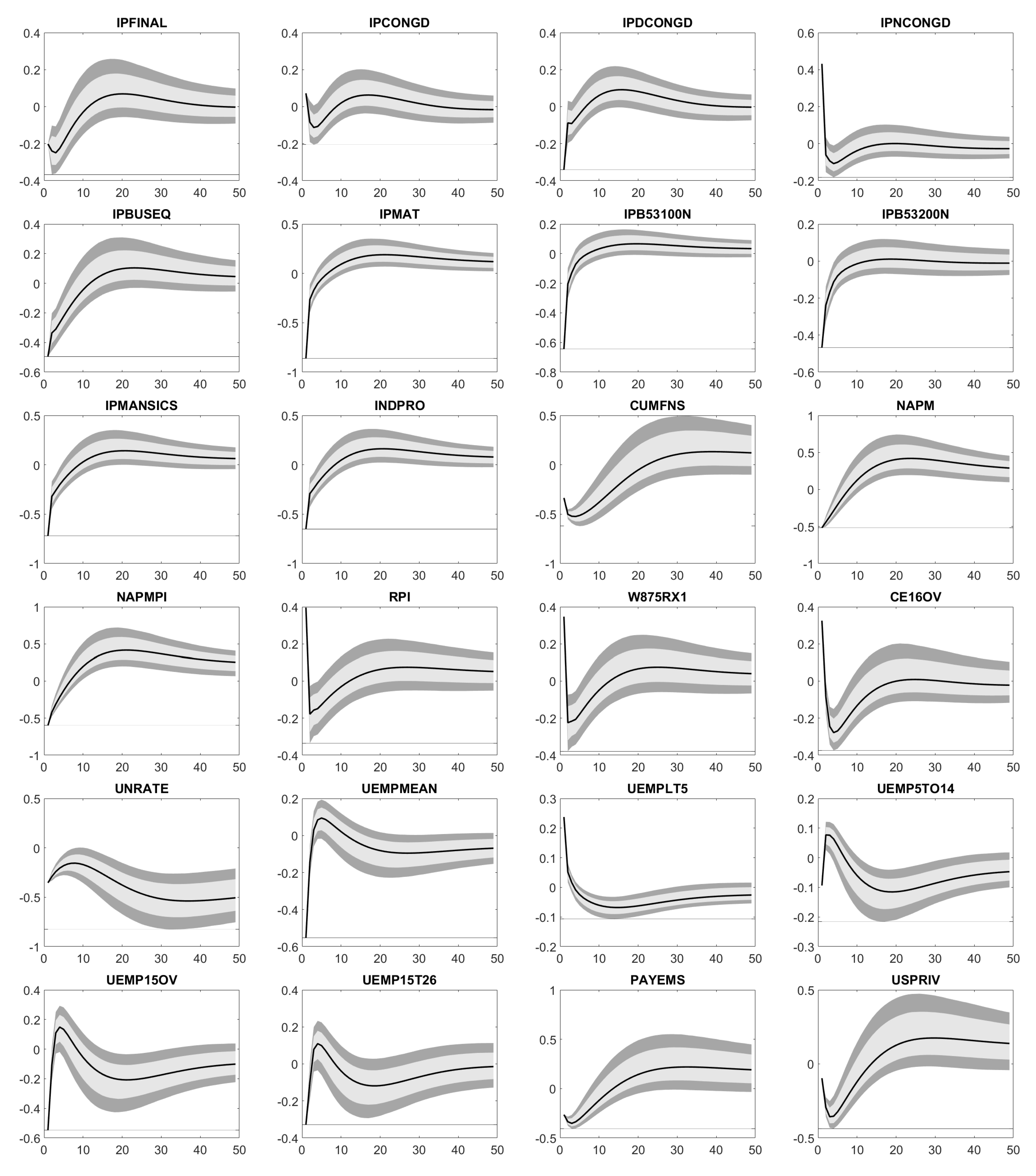
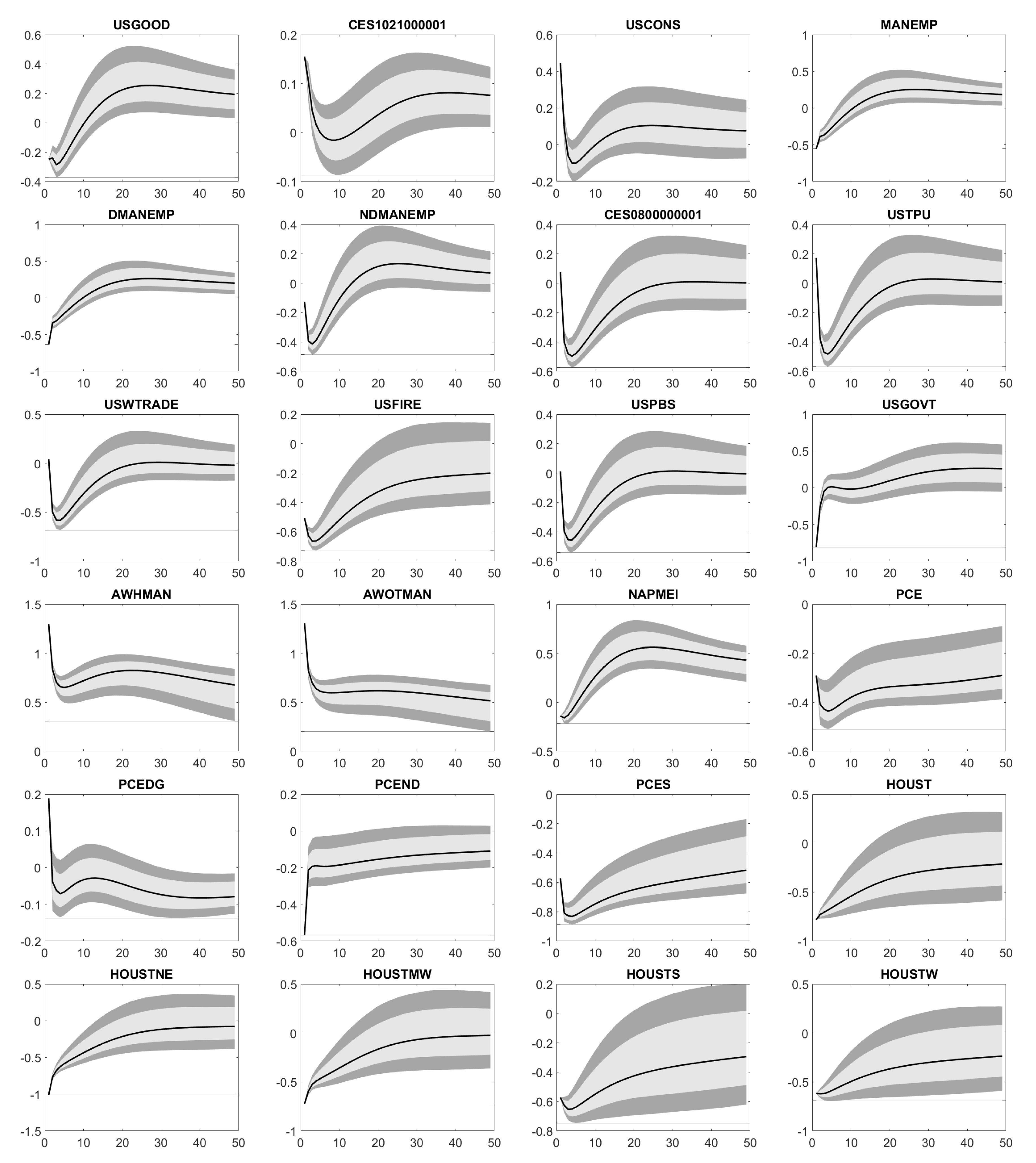
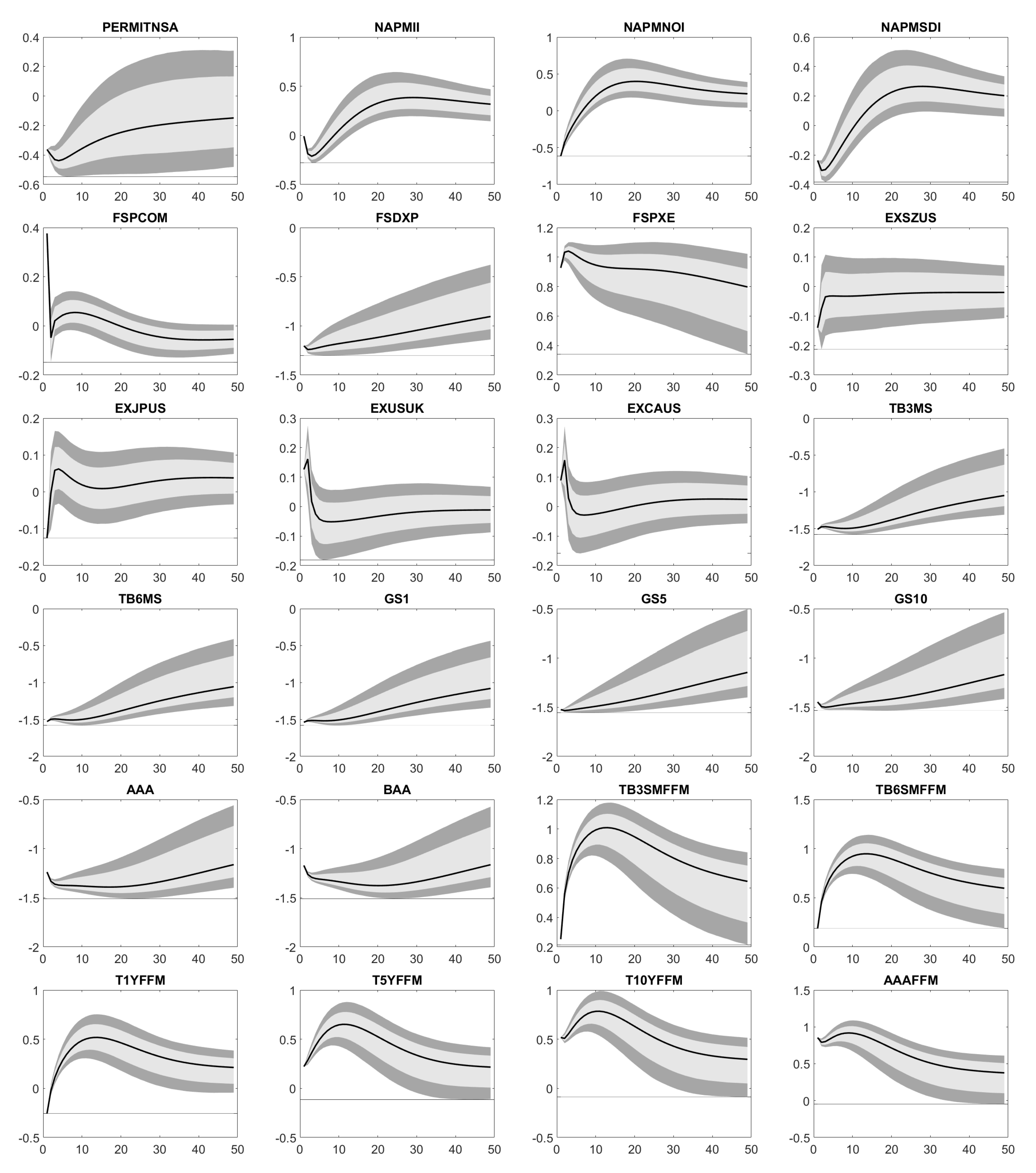
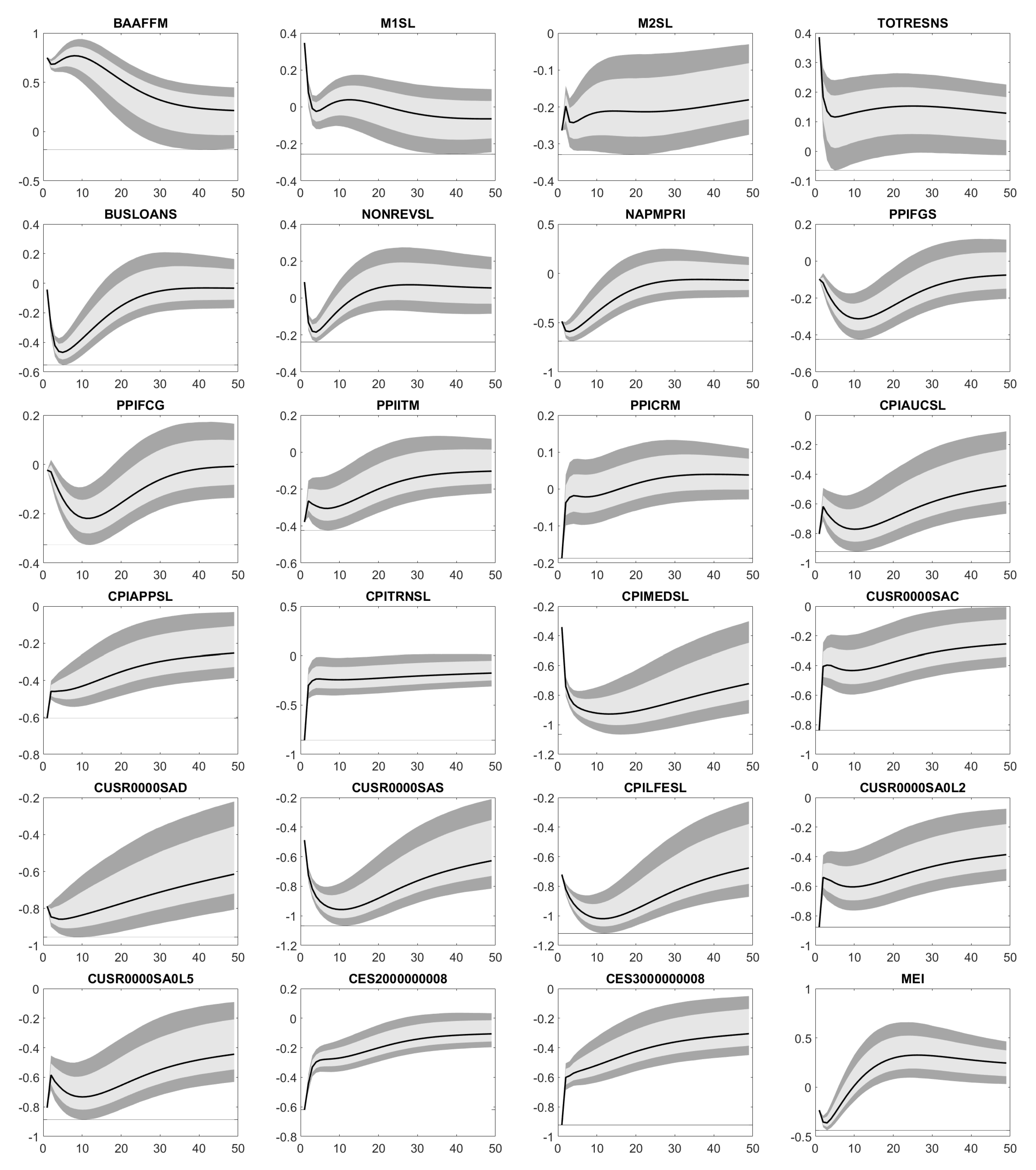
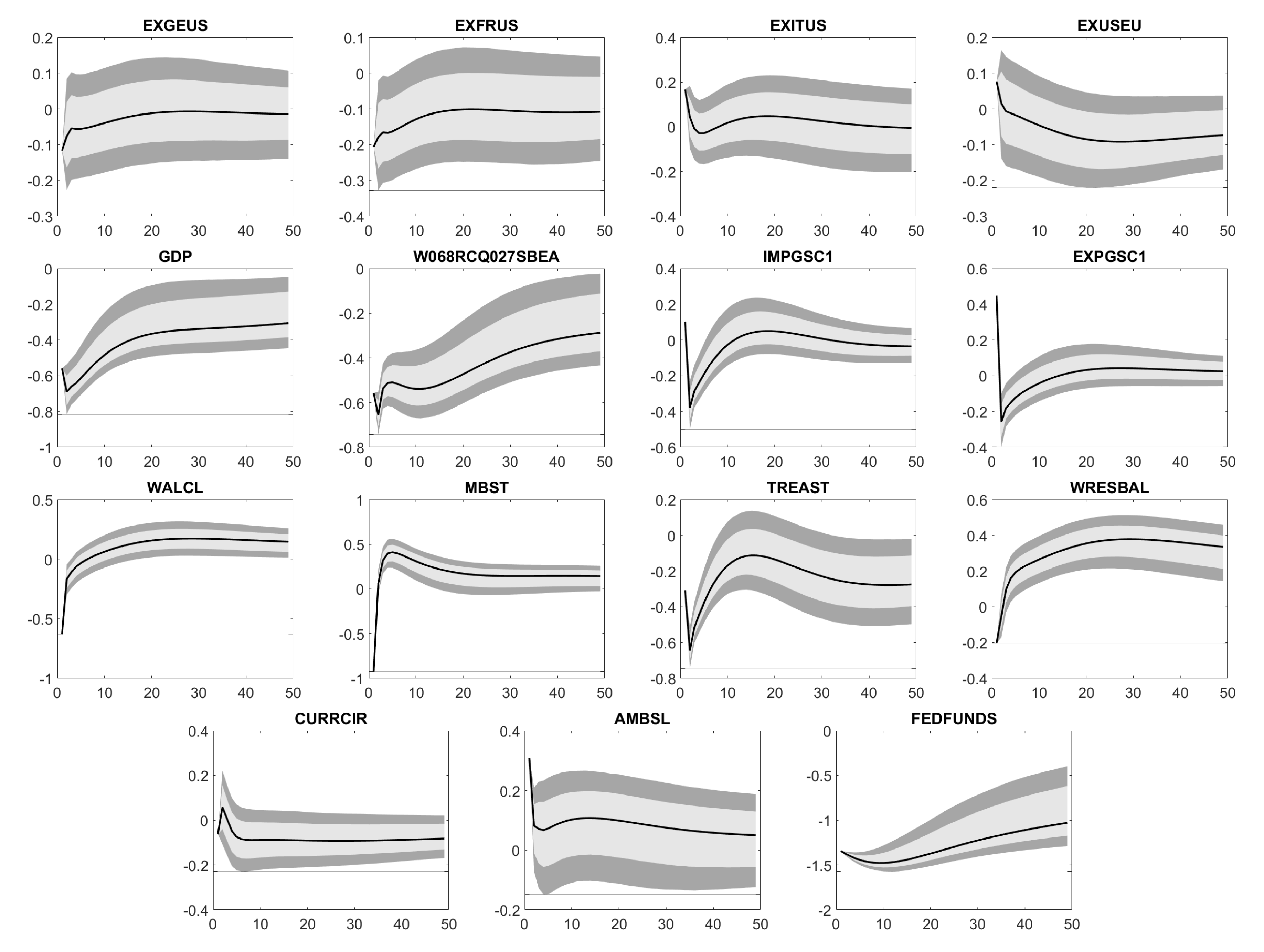
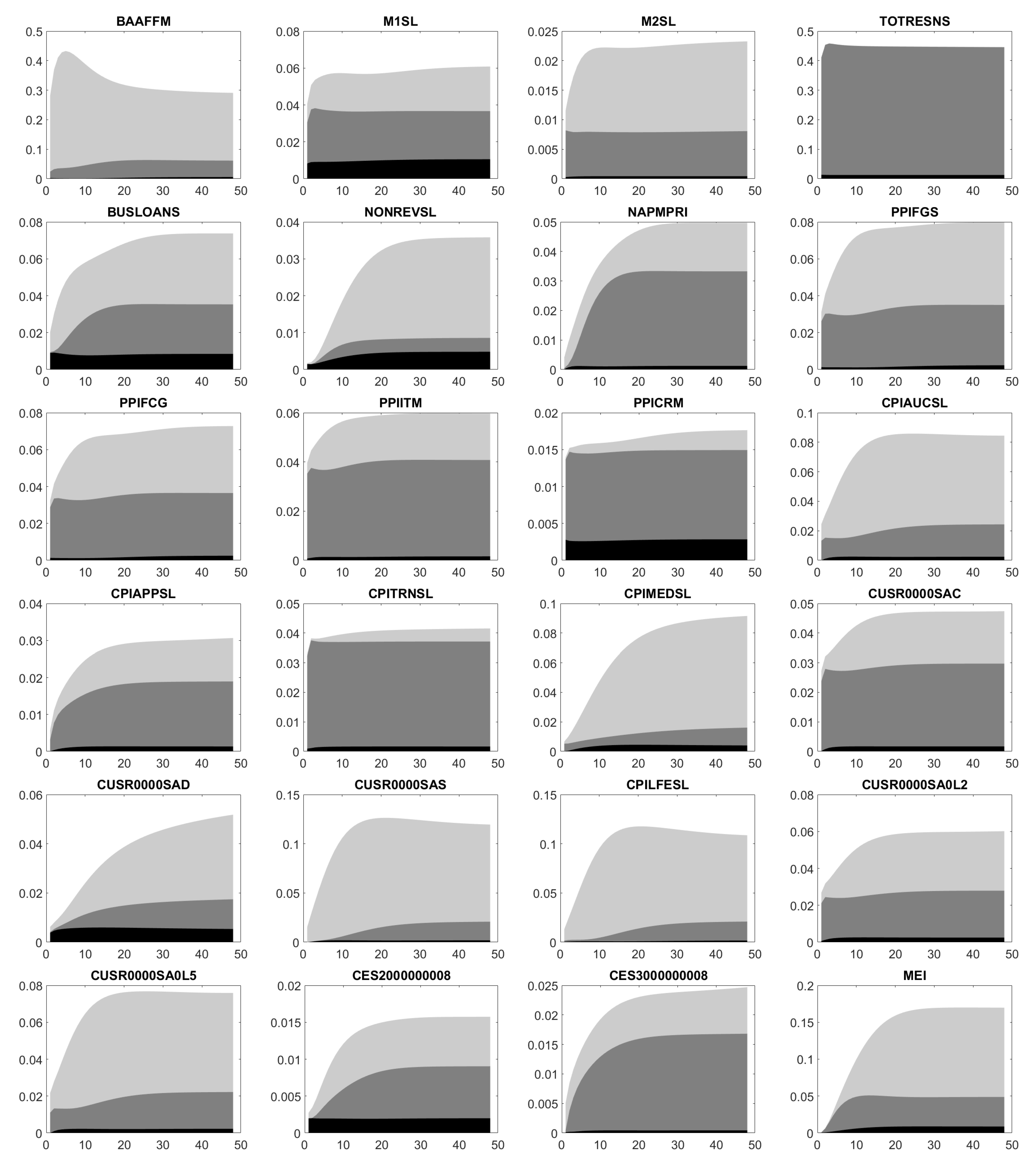
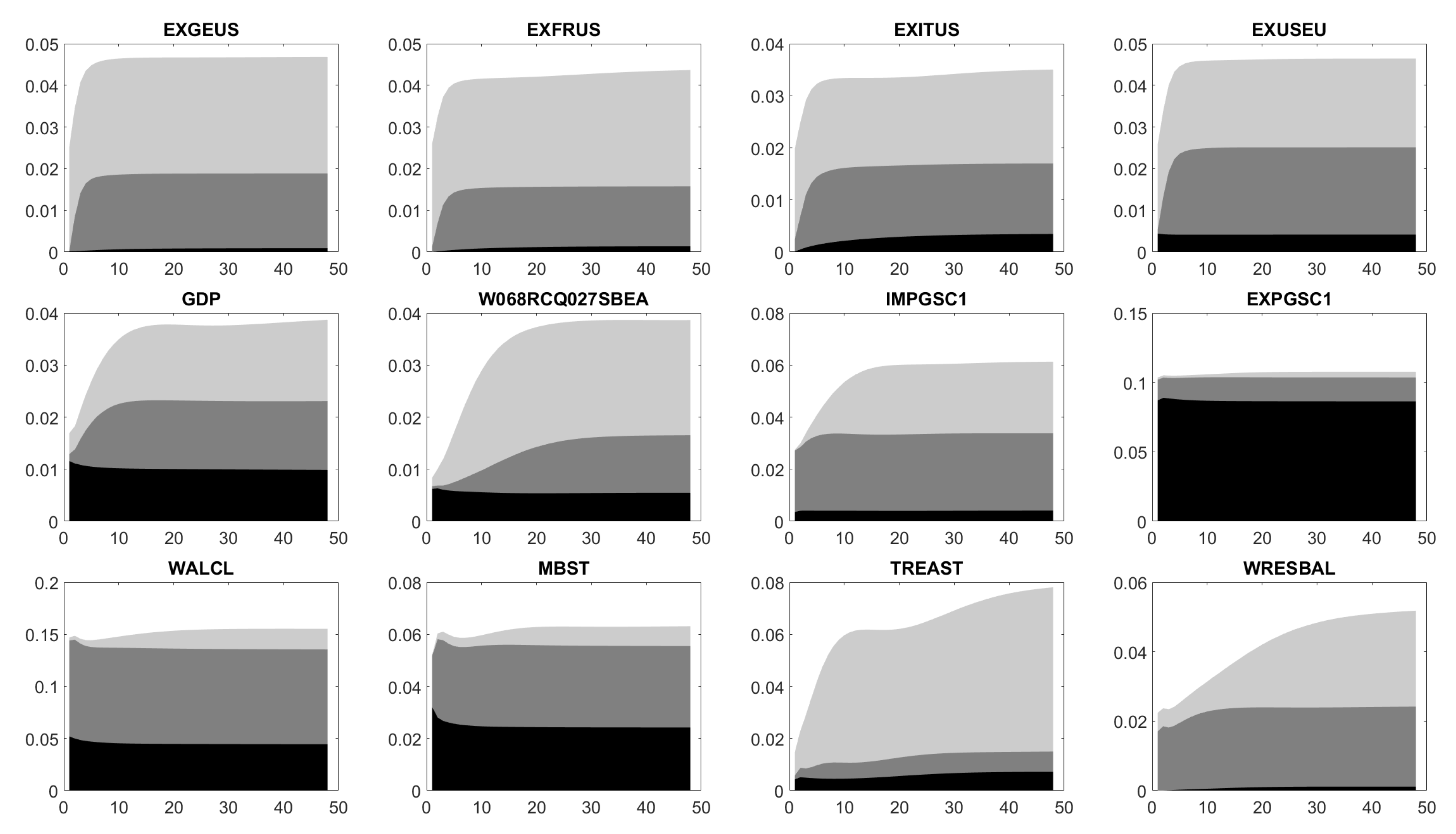
Similar to Bernanke et al. (2005), Bork et al. (2010) and Bork (2015), Figure A1 illustrates the impact of the shock on the standardized variables. Our confidence intervals cover confidence levels of 68% (light gray) and 90% (dark gray) for a time horizon of 48 months. To be more precise, Figure A1 displays for time series or factors :
![Econometrics 07 00031 i004]()

Based on Figure A1, Figure A2, Figure A3, Figure A4 and Figure A5 we conclude: An increase in FEDFUNDS weakens the industrial production (IPFINAL, IPCONGD, IPDCONGD, IPNCONGD, IPBUSEQ, IPMAT, IPB53100N, IPB53200N, IPMANSICS, INDPRO, NAPM, NAPMPI) in the short term without any long-term effects. At the same time, capacities (CUMFNS) are less utilized, personal income (RPI, W875RX1) decreases and unemployment (CE16OV, UNRATE, UEMPMEAN, UEMPLT5, UEMP5TO14, UEMP15OV, UEMP15T26) rises. Similarly, the number of employees across diverse business areas (PAYEMS, USPRIV, USGOOD, CES1021000001, USCONS, MANEMP, DMANEMP, NDMANEMP, CES0800000001, USTPU, USWTRADE, USFIRE, USPBS, USGOVT) and the average production time (AWHMAN, AWOTMAN) decline in the short run. Note, these declines do not necessarily recover. Higher unemployment rates together with lower incomes let the reduced personal expenditures (PCE, PCEDG, PCEND, PCES) appear reasonable.
Housing starts (HOUST, HOUSTNE, HOUSTMW, HOUSTS, HOUSTW, PERMITNSA) are supposed to increase over the next 48 months. Perhaps, this reflects that people are afraid of additional interest rate hikes and therefore, bring such projects forward. Since the Effective Federal Funds Rate applies to the whole US, regional aspects in the case of housing starts do not matter. In the short term, less new orders (NAPMNOI) increase manufacturing inventories (NAPMII), which also confirms a reduction in consumption. In the long run, higher interest rates require companies to offer higher dividends (FSDXP), but boost their costs, too. For example, the same amout of debt calls for higher interest rate payments. In total, the price-earnings ratio (FSPXE) naturally decreases.
Except for EXCAUS and EXITUS, the United States Dollar (USD) becomes stronger compared to foreign currencies (EXSZUS, EXJPUS, EXUSUK, EXGEUS, EXFRUS, EXUSEU). Note that EXITUS is the FX rate between Italian Lira, which the Euro succeeded and USD. Thus, it is not relevant anymore. Here, it is part of our panel data, as EXGEUS, EXFRUS and EXITUS serve as approximations for EXUSEU, before the Euro was introduced on 1 January 1999. A stronger USD may come from an increased demand for USD, when investors increase their exposure to US fixed income products. For instance, US Treasuries’ yields (TB3MS, TB6MS, GS1, GS5, GS10, TB3SMFFM, TB6SMFFM, T1YFFM, T5YFFM, T10YFFM) and corporate bond spreads (AAA, BAA, AAAFFM, BAAFFM) follow an increase in FEDFUNDS.
The drops in M1SL, TOTRESNS, BUSLOANS and NONREVSL let the available liquidity shrink, what the US Federal Reserve is exactly aiming at. In addition, prices and inflation (NAPMPRI, PPIFGS, PPIITM, PPICRM, CPIAUCSL, CPIAPPSL, CPITRNSL, CUSR0000SAC, CUSR0000SAD, CUSR0000SA0L2, CUSR0000SA0L5) climb in the long term such that the US economy eventually leaves its crisis mode and comes back to normal. This assumption is supported by the raising composite leading indicator MEI and GDP. Although there are no long-term effects on the export and import of goods and serices (EXPGSC1, IMPGSC1), both decrease. The reduced export might arise from the strong USD, which makes US products more expensive abroad. By contrast, the strong USD reduces the USD prices of foreign products. Hence, the drop in USD prices is not balanced by a bigger amount of imported products. Finally, assets and reserves of the Federal Reserve (WALCL, MBST, TREAST, WRESBAL, AMBSL) possibly change.
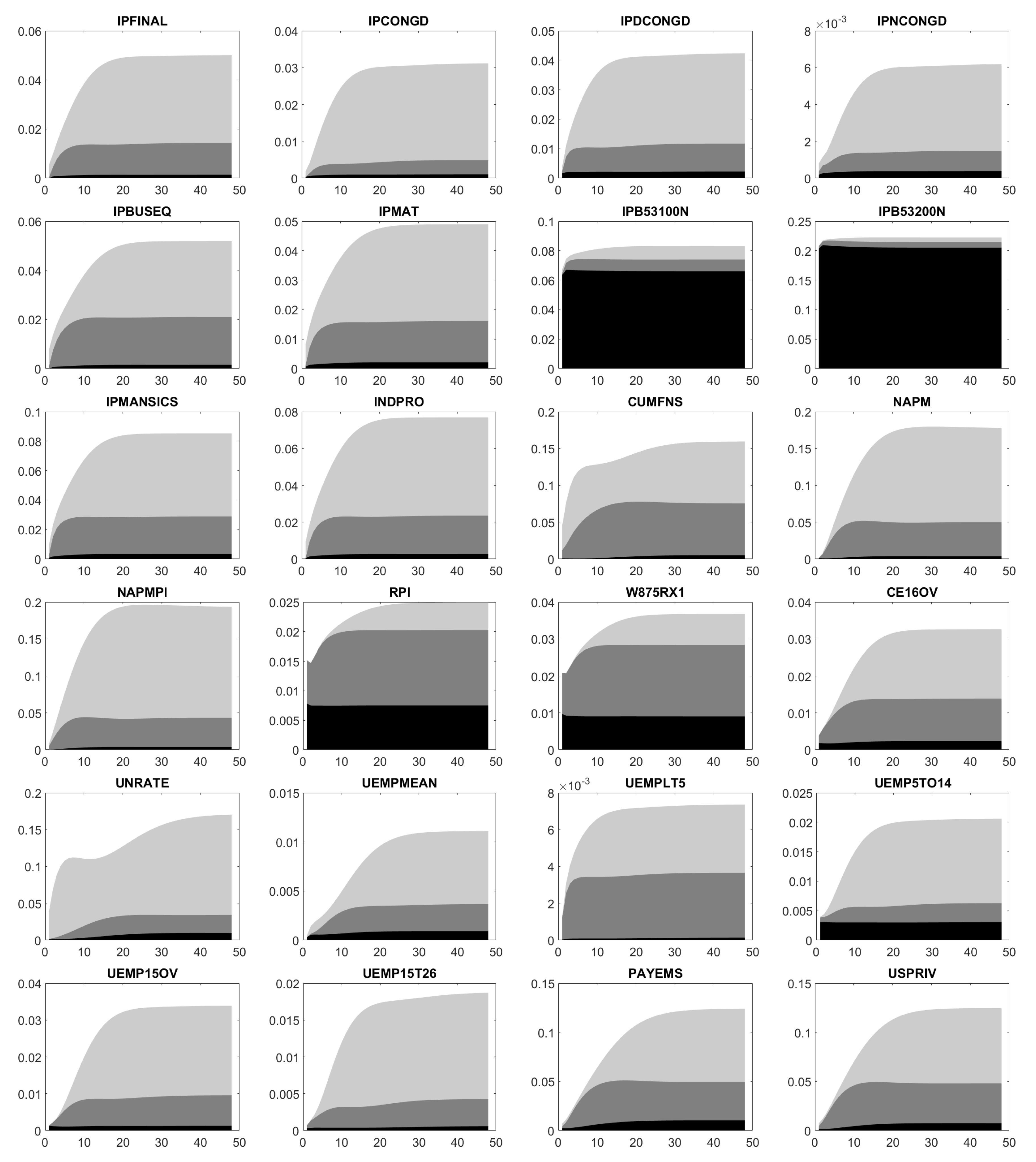
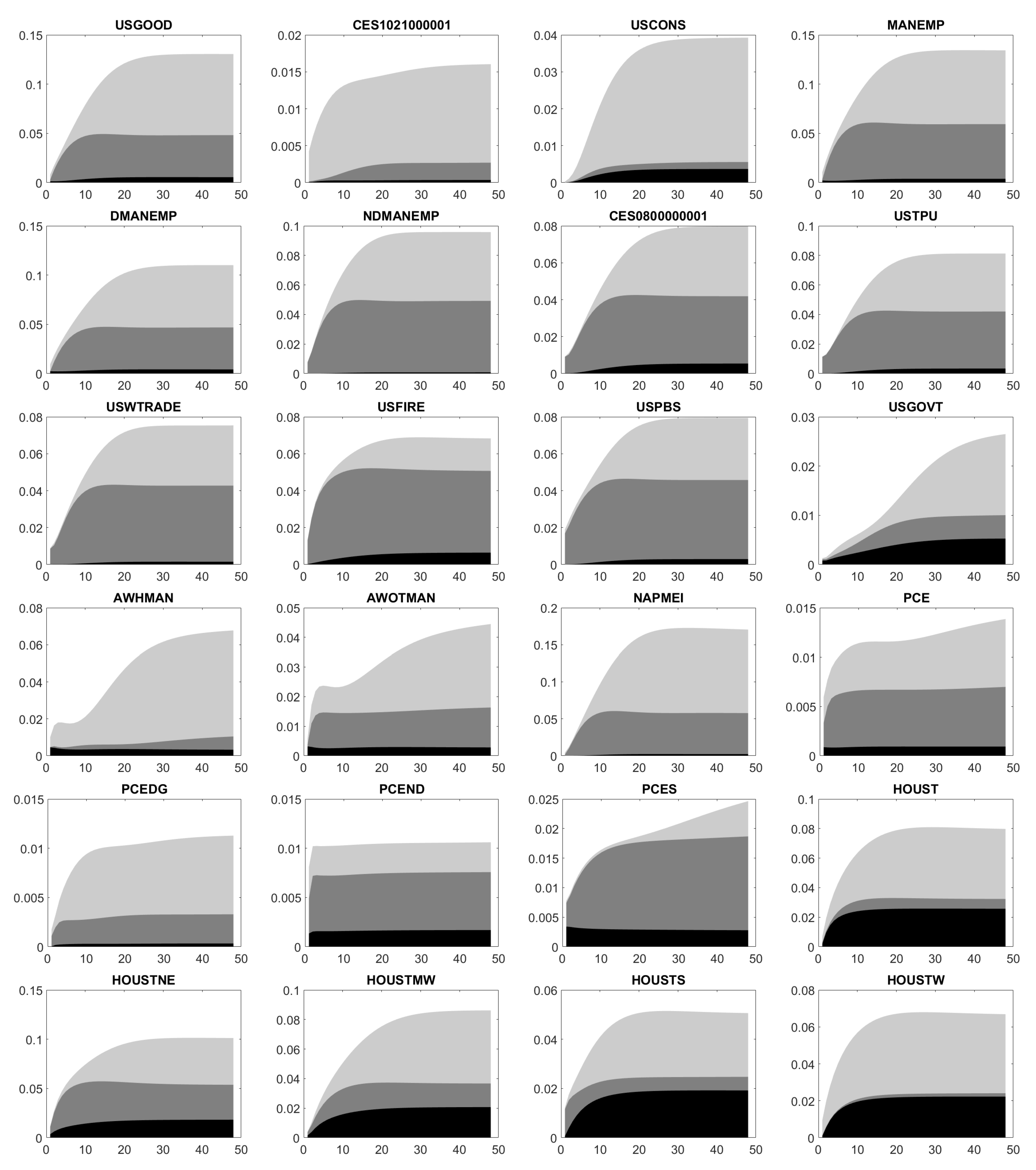
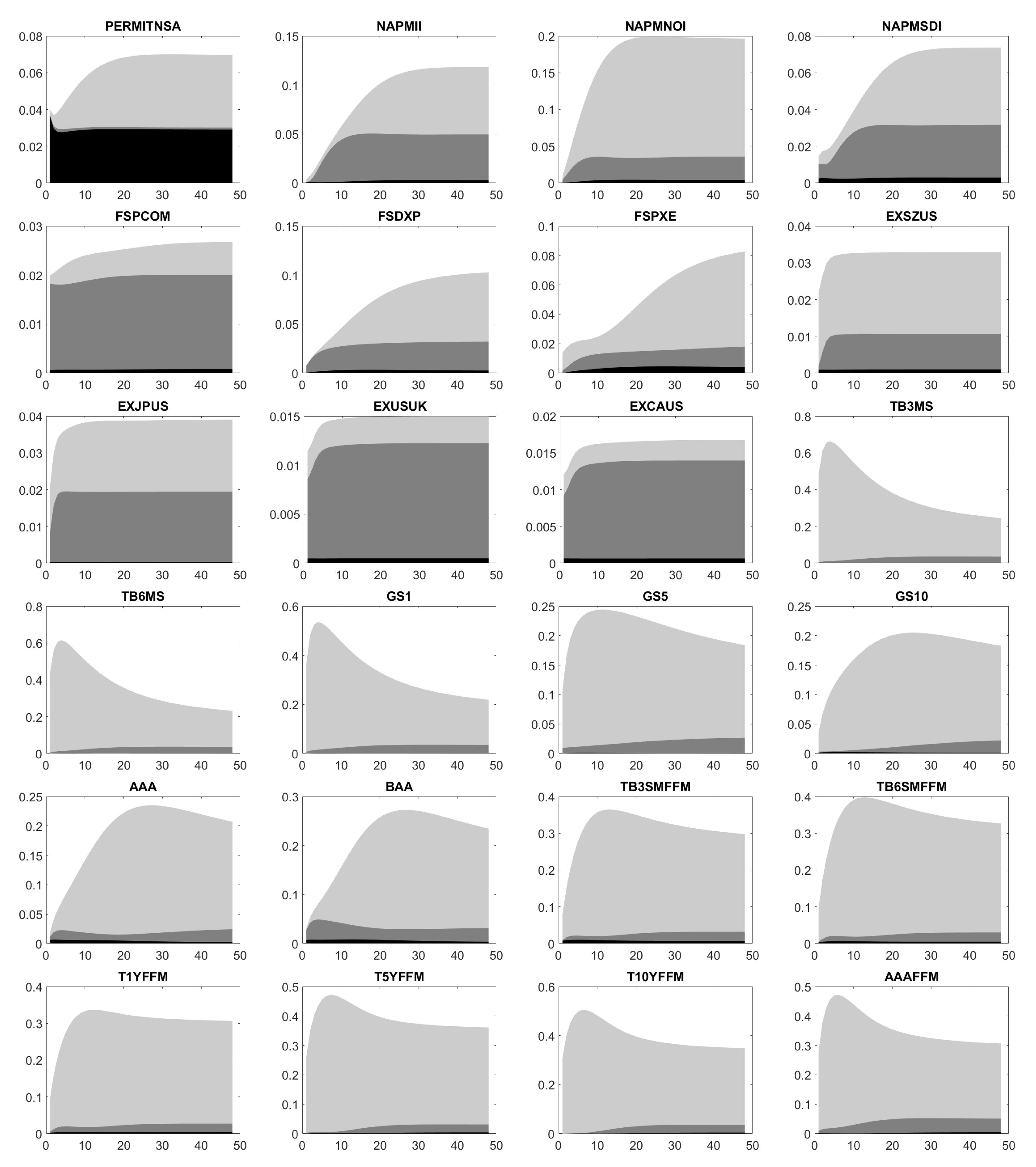
Figure A6, Figure A7, Figure A8, Figure A9 and Figure A10 illustrate the estimated FEVD. Here, each plot displays the innovations in CURRCIR, AMBSL and FEDFUNDS. Then, we conclude: First, total contribution as well as single ones in CURRCIR, AMBSL and FEDFUNDS considerably change over time and depend on the chosen variable. Second, CURRCIR innovations heavily affect the forecast error variance of IPB53100N, IPB53200N, RPI, W875RX1, HOUST, HOUSTS, HOUSTW, PERMITNSA, EXPGSC1 and MBST, which rank among the macroeconomic data. For AMBSL, we have a scattered picture. On the one hand, its shocks drive the forecast error variance of production data (IPFINAL, IPBUSEQ, IPMAT, INDPRO, CUMFNS, GDP, IMPGSC1), income (RPI, W875RX1), employment (PAYEMS, USGOOD, MANEMP, NDMANEMP, CES0800000001, USTPU, USWTRADE, USFIRE, USPBS), consumption (PCE, PCEND, PCES) and inflation (NAPMPRI, PPIFGS, PPIFCG, PPIITM, PPICRM, CPIAPPSL, CPITRNSL, CUSR0000SAC, CES3000000008). On the other hand, those also affect the forecast error variance of financial data (FSPCOM, EXJPUS, EXUSUK, EXCAUS, EXGEUS, EXFRUS, EXITUS, EXUSEU) and liquidity measures (M1SL, M2SL, TOTRESNS, BUSLOANS). Similarly, FEDFUNDS shocks move all areas, in particular, US Treasuries (TB3MS, TB6MS, GS1, GS5, GS10, TB3SMFFM, TB6SMFFM, T1YFFM, T5YFFM, T10YFFM) and corporate bond spreads (AAA, BAA, AAAFFM, BAAFFM). Besides the observed factors, the idiosyncratic error variance usually represents an important driver of the forecast error variance.
5. Conclusions and Final Remarks
This article considers the estimation of FAVARs, when the underlying panel data is incomplete. Thereby, incompleteness arises from the inclusion of mixed-frequency information and the absence of single values. Besides the panel data, a FAVAR comprises observable variables which, together with hidden factors, drive the joint factor dynamics. So far, the presented estimation method calls for full time series of the observable factors. Therefore, an extension to incomplete observed factors is a direction of the future research.
Within a maximum likelihood framework, a fully parametric two-step routine simultaneously estimates unknown model parameters and missing data. In a nutshell, two expectation-maximization algorithms are alternately applied until a pre-specified convergence criterion is reached. The first derives complete data from the observations and latest parameter estimates, whereas the second re-estimates the parameters, whenever the complete data changes. In the scope of a MC simulation study, the superior estimation quality of the suggested approach compared to already existing methods is confirmed.
The main contributions of this paper to the existing literature are as follows: First, we extend the FAVAR of Bernanke et al. (2005) to incomplete panel data. Marcellino and Sivec (2016) did the same, but their estimation method requires the observable factor components to be part of the panel data. By contrast, we modify the Kalman filter such that it takes into account that the factors are partially observed and so, can relax their restriction.
Second, the presented estimation method adds flexibility to the loadings matrix. As mentioned before, in Bork (2009) the observable factors are included in the panel data. In doing so, they occupy certain positions which calls for a specific shape of the loadings matrix, but allows Bork (2009) to apply estimation methods for dynamic approximate factor model for the estimation of the FAVAR of Bernanke et al. (2005). A main advantage of our new Kalman filter is the fact that we have to choose a few loadings constraints to ensure parameter uniqueness, but there is no need for a special structure of the loadings matrix.
Third, we explicitly separate the observable factors from latent ones. Because of this, we determine all results for the general case of an arbitrary autoregressive oder . That is, we do not use the argument that any VAR of order can be traced back to a VAR and do not treat this simplest case. Therefore, our results can be directly applied without any adjustments.
Fourth, the inclusion of mixed-frequency data enables us to investigate the impact of the monetary policy on quarterly indicators like GDP. For instance, our empirical study considers the US economy. Based on a sample, which covers 108 macroeconomic variables and a three-dimensional vector of observable factors over a period from January 1959 until October 2015, we come to the conclusion that GDP gains from an increase in the Effectice Federal Funds Rate by 0.25% in the long term.
In the recent literature, FAVARs were primarily used in the context of monetary policy. However, the extraction of relevant information from big data is already an overarching topic. Therefore, the application of FAVARs to areas beyond monetary policy (e.g., customer behavior/churn, macroeconomic forecasting, diagnosis of diseases) based on the proposed estimation method could be part of the future research. In addition, our approach may be extended to serially correlated errors such that the overall framework admits cross-sectionally and serially correlated error terms.
In the case of monetary policy, a comprehensive comparison of the presented approach with Multivariate State-space Time-varying Parameter VARs (MVSS-TVP-VARs), Dynamic Stochastic General Equilibrium Models (DSGEs), Bayesian VARs and their extensions as in Bekiros and Paccagnini (2014, 2015) could be performed. In this regard, some of them must be extended to ragged panel data in a first step. Furthermore, the seemingly unrelated time series equations for MVSS-TVP-VARs in Bekiros and Paccagnini (2015) rely on the univariate version of the standard Kalman Filter and consider the observable variables independently. Finally, the vector must be part of the panel data . Therefore, the most important direction of the future research could be the combination of the models in Bekiros and Paccagnini (2014, 2015) with our proposed Kalman Filter for the joint vector based on the panel data .
Author Contributions
M.L. and F.R. analyzed data and drafted a first estimation method. A.M. and F.R. further developed the model and associated estimation procedure. M.L. and F.R. performed the complete computational implementation. All three authors wrote the paper.
Funding
The PhD position of Franz Ramsauer at Technical University of Munich was third-party funded by Pioneer Investments, which is now part of Amundi Asset Management. Otherwise, this research received no external funding.
Acknowledgments
The authors want to thank the editor and the two anonymous reviewers for their very helpful suggestions, which essentially contributed to the improvement of our manuscript. The authors gratefully acknowledge Alec Chrystal for his help on monetary policy references. Franz Ramsauer gratefully acknowledges the support of Pioneer Investments, which is now part of Amundi Asset Management, during his doctoral phase.
Conflicts of Interest
The authors declare no conflict of interest. The sponsors had no role in the design of the study, in the collection, analyses, or interpretation of data, in the writing of the manuscript and in the decision to publish the results.
Abbreviations
The following abbreviations are used in this manuscript:
| AIC | Akaike Information Criterion |
| bp | basis point |
| DFM | Dynamic Factor Model |
| EM | Expectation-Maximization Algorithm |
| FAVAR | Factor-Augmented Vector Autoregression Model |
| FEVD | Forecast Error Variance Decomposition |
| FEDFUNDS | Effective Federal Funds Rate |
| FX | Foreign Exchange |
| GDP | Gross Domestic Product |
| iid | identically and independently distributed |
| IRF | Impulse Response Function |
| KF | Kalman Filter |
| KS | Kalman Smoother |
| MC | Monte Carlo |
| MLE | Maximum-Likelihood Estimation |
| NSA | Not Seasonally Adjusted |
| OLS | Ordinary Least Squares Regression |
| PCA | Principal Component Analysis |
| SA | Seasonally Adjusted |
| UK | United Kingdom |
| UNRATE | Unemployment Rate |
| URL | Uniform Resource Locator |
| US | United States |
| USD | United States Dollar |
| VAR | Vector Autoregression Model |
Appendix A. Algorithms
| Algorithm A1: Kalman Filter for FAVARs with complete panel data |
 |
| Algorithm A2: Estimation of FAVARs with constraints for incomplete panel data |
 |
Appendix B. Simulation Results

Table A1.
Means of trace based on hidden factors for random FAVARs using PCA and OLS.
| Stock | Stock/Flow (Average) | Stock/Change in Flow (Average) | |||||||||||
|---|---|---|---|---|---|---|---|---|---|---|---|---|---|
| ratio of missing data | ratio of missing data | ratio of missing data | |||||||||||
| N | T | 0% | 5% | 10% | 15% | 0% | 5% | 10% | 15% | 0% | 5% | 10% | 15% |
| 80 | 600 | 0.49 | 0.49 | 0.48 | 0.49 | 0.49 | 0.49 | 0.48 | 0.50 | 0.49 | 0.49 | 0.49 | 0.50 |
| 80 | 800 | 0.49 | 0.49 | 0.50 | 0.49 | 0.50 | 0.49 | 0.48 | 0.50 | 0.49 | 0.49 | 0.49 | 0.48 |
| 100 | 600 | 0.49 | 0.50 | 0.50 | 0.49 | 0.49 | 0.49 | 0.49 | 0.49 | 0.49 | 0.49 | 0.49 | 0.49 |
| 100 | 800 | 0.50 | 0.50 | 0.49 | 0.49 | 0.49 | 0.50 | 0.49 | 0.49 | 0.49 | 0.49 | 0.50 | 0.50 |
| 120 | 600 | 0.50 | 0.49 | 0.50 | 0.50 | 0.50 | 0.49 | 0.48 | 0.50 | 0.50 | 0.49 | 0.50 | 0.48 |
| 120 | 800 | 0.49 | 0.50 | 0.49 | 0.50 | 0.49 | 0.49 | 0.50 | 0.49 | 0.49 | 0.49 | 0.49 | 0.49 |
| 80 | 600 | 0.74 | 0.74 | 0.74 | 0.74 | 0.74 | 0.74 | 0.74 | 0.73 | 0.74 | 0.74 | 0.73 | 0.73 |
| 80 | 800 | 0.74 | 0.74 | 0.74 | 0.74 | 0.74 | 0.74 | 0.74 | 0.73 | 0.74 | 0.74 | 0.73 | 0.73 |
| 100 | 600 | 0.75 | 0.76 | 0.76 | 0.75 | 0.76 | 0.75 | 0.75 | 0.75 | 0.76 | 0.75 | 0.75 | 0.74 |
| 100 | 800 | 0.75 | 0.76 | 0.75 | 0.75 | 0.75 | 0.75 | 0.75 | 0.74 | 0.75 | 0.75 | 0.75 | 0.74 |
| 120 | 600 | 0.76 | 0.77 | 0.76 | 0.76 | 0.77 | 0.77 | 0.76 | 0.76 | 0.77 | 0.77 | 0.76 | 0.75 |
| 120 | 800 | 0.76 | 0.76 | 0.76 | 0.76 | 0.76 | 0.76 | 0.76 | 0.75 | 0.76 | 0.76 | 0.75 | 0.75 |
| 80 | 600 | 0.55 | 0.56 | 0.57 | 0.56 | 0.56 | 0.56 | 0.56 | 0.56 | 0.55 | 0.56 | 0.56 | 0.55 |
| 80 | 800 | 0.56 | 0.56 | 0.56 | 0.56 | 0.55 | 0.56 | 0.55 | 0.56 | 0.55 | 0.55 | 0.55 | 0.55 |
| 100 | 600 | 0.57 | 0.56 | 0.57 | 0.56 | 0.56 | 0.57 | 0.56 | 0.56 | 0.56 | 0.57 | 0.57 | 0.56 |
| 100 | 800 | 0.56 | 0.56 | 0.57 | 0.57 | 0.56 | 0.57 | 0.57 | 0.56 | 0.56 | 0.56 | 0.56 | 0.55 |
| 120 | 600 | 0.57 | 0.57 | 0.57 | 0.58 | 0.57 | 0.57 | 0.57 | 0.57 | 0.57 | 0.57 | 0.57 | 0.56 |
| 120 | 800 | 0.56 | 0.57 | 0.57 | 0.57 | 0.57 | 0.56 | 0.57 | 0.57 | 0.57 | 0.57 | 0.57 | 0.56 |
| 80 | 600 | 0.79 | 0.79 | 0.79 | 0.78 | 0.79 | 0.79 | 0.78 | 0.78 | 0.79 | 0.79 | 0.78 | 0.77 |
| 80 | 800 | 0.79 | 0.79 | 0.78 | 0.78 | 0.79 | 0.79 | 0.78 | 0.78 | 0.79 | 0.79 | 0.78 | 0.78 |
| 100 | 600 | 0.80 | 0.80 | 0.80 | 0.79 | 0.80 | 0.80 | 0.80 | 0.80 | 0.81 | 0.81 | 0.79 | 0.79 |
| 100 | 800 | 0.81 | 0.80 | 0.80 | 0.80 | 0.81 | 0.80 | 0.80 | 0.80 | 0.80 | 0.80 | 0.79 | 0.79 |
| 120 | 600 | 0.81 | 0.81 | 0.81 | 0.81 | 0.81 | 0.81 | 0.81 | 0.80 | 0.81 | 0.81 | 0.80 | 0.80 |
| 120 | 800 | 0.82 | 0.82 | 0.81 | 0.81 | 0.82 | 0.81 | 0.81 | 0.80 | 0.81 | 0.81 | 0.81 | 0.80 |
| 80 | 600 | 0.65 | 0.65 | 0.65 | 0.65 | 0.65 | 0.65 | 0.65 | 0.65 | 0.65 | 0.65 | 0.65 | 0.65 |
| 80 | 800 | 0.65 | 0.65 | 0.65 | 0.65 | 0.66 | 0.66 | 0.65 | 0.65 | 0.65 | 0.65 | 0.65 | 0.65 |
| 100 | 600 | 0.66 | 0.66 | 0.66 | 0.65 | 0.66 | 0.66 | 0.66 | 0.66 | 0.66 | 0.66 | 0.65 | 0.66 |
| 100 | 800 | 0.67 | 0.66 | 0.66 | 0.67 | 0.66 | 0.66 | 0.66 | 0.65 | 0.66 | 0.66 | 0.66 | 0.66 |
| 120 | 600 | 0.67 | 0.67 | 0.67 | 0.67 | 0.67 | 0.67 | 0.66 | 0.66 | 0.67 | 0.67 | 0.66 | 0.66 |
| 120 | 800 | 0.67 | 0.67 | 0.67 | 0.67 | 0.67 | 0.67 | 0.67 | 0.66 | 0.67 | 0.67 | 0.67 | 0.66 |
The displayed means are derived from 500 MC simulations for known dimensions K and p. For incomplete time series a stock variable is assumed; For incomplete data, and time series are stock and flow (average formulation) variables, respectively; For incomplete data, and time series serve as stock or change in flow (average formulaton) variables.
Table A2.
Means of trace based on hidden factors for random FAVARs using standard KF and KS, when complete panel data relies on estimated factors instead of observed variables.
Table A2.
Means of trace based on hidden factors for random FAVARs using standard KF and KS, when complete panel data relies on estimated factors instead of observed variables.
| Stock | Stock/Flow (Average) | Stock/Change in Flow (Average) | |||||||||||
|---|---|---|---|---|---|---|---|---|---|---|---|---|---|
| ratio of missing data | ratio of missing data | ratio of missing data | |||||||||||
| N | T | 0% | 5% | 10% | 15% | 0% | 5% | 10% | 15% | 0% | 5% | 10% | 15% |
| 80 | 600 | 0.46 | 0.46 | 0.45 | 0.46 | 0.46 | 0.46 | 0.45 | 0.44 | 0.46 | 0.47 | 0.45 | 0.43 |
| 80 | 800 | 0.47 | 0.46 | 0.47 | 0.46 | 0.47 | 0.47 | 0.45 | 0.45 | 0.47 | 0.46 | 0.43 | 0.43 |
| 100 | 600 | 0.46 | 0.47 | 0.48 | 0.46 | 0.47 | 0.47 | 0.44 | 0.40 | 0.47 | 0.47 | 0.41 | 0.40 |
| 100 | 800 | 0.48 | 0.48 | 0.46 | 0.47 | 0.46 | 0.47 | 0.44 | 0.41 | 0.46 | 0.47 | 0.43 | 0.40 |
| 120 | 600 | 0.48 | 0.47 | 0.48 | 0.47 | 0.48 | 0.47 | 0.42 | 0.42 | 0.48 | 0.46 | 0.42 | 0.40 |
| 120 | 800 | 0.47 | 0.48 | 0.47 | 0.48 | 0.47 | 0.47 | 0.45 | 0.40 | 0.47 | 0.46 | 0.42 | 0.42 |
| 80 | 600 | 0.68 | 0.67 | 0.67 | 0.66 | 0.68 | 0.67 | 0.65 | 0.63 | 0.68 | 0.67 | 0.64 | 0.56 |
| 80 | 800 | 0.68 | 0.67 | 0.67 | 0.66 | 0.68 | 0.67 | 0.66 | 0.63 | 0.68 | 0.67 | 0.64 | 0.57 |
| 100 | 600 | 0.70 | 0.69 | 0.69 | 0.67 | 0.70 | 0.69 | 0.67 | 0.63 | 0.70 | 0.69 | 0.66 | 0.56 |
| 100 | 800 | 0.69 | 0.69 | 0.68 | 0.68 | 0.70 | 0.69 | 0.68 | 0.63 | 0.70 | 0.69 | 0.66 | 0.57 |
| 120 | 600 | 0.71 | 0.70 | 0.70 | 0.69 | 0.71 | 0.71 | 0.69 | 0.63 | 0.71 | 0.70 | 0.66 | 0.56 |
| 120 | 800 | 0.71 | 0.70 | 0.70 | 0.70 | 0.71 | 0.70 | 0.69 | 0.65 | 0.71 | 0.70 | 0.66 | 0.57 |
| 80 | 600 | 0.38 | 0.37 | 0.37 | 0.35 | 0.38 | 0.37 | 0.35 | 0.31 | 0.38 | 0.37 | 0.33 | 0.29 |
| 80 | 800 | 0.38 | 0.38 | 0.36 | 0.35 | 0.38 | 0.36 | 0.34 | 0.31 | 0.37 | 0.36 | 0.32 | 0.29 |
| 100 | 600 | 0.41 | 0.39 | 0.38 | 0.37 | 0.41 | 0.39 | 0.36 | 0.31 | 0.40 | 0.38 | 0.33 | 0.30 |
| 100 | 800 | 0.40 | 0.39 | 0.38 | 0.37 | 0.40 | 0.39 | 0.36 | 0.31 | 0.40 | 0.38 | 0.33 | 0.30 |
| 120 | 600 | 0.42 | 0.41 | 0.40 | 0.39 | 0.42 | 0.41 | 0.36 | 0.31 | 0.42 | 0.40 | 0.33 | 0.28 |
| 120 | 800 | 0.41 | 0.41 | 0.40 | 0.39 | 0.42 | 0.40 | 0.37 | 0.31 | 0.42 | 0.40 | 0.34 | 0.29 |
| 80 | 600 | 0.75 | 0.74 | 0.74 | 0.73 | 0.75 | 0.74 | 0.73 | 0.69 | 0.75 | 0.74 | 0.73 | 0.65 |
| 80 | 800 | 0.75 | 0.74 | 0.73 | 0.73 | 0.75 | 0.75 | 0.73 | 0.69 | 0.75 | 0.74 | 0.72 | 0.66 |
| 100 | 600 | 0.77 | 0.76 | 0.76 | 0.74 | 0.76 | 0.76 | 0.74 | 0.70 | 0.77 | 0.76 | 0.72 | 0.65 |
| 100 | 800 | 0.77 | 0.76 | 0.75 | 0.75 | 0.77 | 0.76 | 0.75 | 0.71 | 0.76 | 0.76 | 0.73 | 0.67 |
| 120 | 600 | 0.78 | 0.78 | 0.76 | 0.76 | 0.78 | 0.77 | 0.74 | 0.70 | 0.78 | 0.77 | 0.73 | 0.65 |
| 120 | 800 | 0.78 | 0.78 | 0.77 | 0.76 | 0.78 | 0.77 | 0.75 | 0.71 | 0.78 | 0.77 | 0.74 | 0.66 |
| 80 | 600 | 0.54 | 0.52 | 0.52 | 0.51 | 0.55 | 0.54 | 0.50 | 0.47 | 0.54 | 0.52 | 0.50 | 0.45 |
| 80 | 800 | 0.54 | 0.52 | 0.53 | 0.52 | 0.55 | 0.54 | 0.49 | 0.48 | 0.55 | 0.52 | 0.50 | 0.47 |
| 100 | 600 | 0.56 | 0.55 | 0.53 | 0.52 | 0.56 | 0.54 | 0.51 | 0.47 | 0.56 | 0.54 | 0.48 | 0.45 |
| 100 | 800 | 0.57 | 0.55 | 0.55 | 0.54 | 0.55 | 0.55 | 0.52 | 0.46 | 0.55 | 0.54 | 0.50 | 0.45 |
| 120 | 600 | 0.57 | 0.57 | 0.56 | 0.55 | 0.57 | 0.57 | 0.50 | 0.45 | 0.58 | 0.55 | 0.49 | 0.42 |
| 120 | 800 | 0.57 | 0.57 | 0.55 | 0.55 | 0.57 | 0.57 | 0.52 | 0.46 | 0.57 | 0.56 | 0.49 | 0.43 |
The displayed means are derived from 500 MC simulations for known dimensions K and p. For incomplete time series a stock variable is assumed; For incomplete data, and time series are stock and flow (average formulation) variables, respectively; For incomplete data, and time series serve as stock or change in flow (average formulaton) variables.
Table A3.
Means of trace based on hidden factors for random FAVARs using standard KF and KS, when complete panel data takes observed variables into account.
Table A3.
Means of trace based on hidden factors for random FAVARs using standard KF and KS, when complete panel data takes observed variables into account.
| Stock | Stock/Flow (Average) | Stock/Change in Flow (Average) | |||||||||||
|---|---|---|---|---|---|---|---|---|---|---|---|---|---|
| ratio of missing data | ratio of missing data | ratio of missing data | |||||||||||
| N | T | 0% | 5% | 10% | 15% | 0% | 5% | 10% | 15% | 0% | 5% | 10% | 15% |
| 80 | 600 | 0.46 | 0.46 | 0.45 | 0.46 | 0.46 | 0.46 | 0.46 | 0.47 | 0.46 | 0.47 | 0.46 | 0.46 |
| 80 | 800 | 0.47 | 0.46 | 0.47 | 0.47 | 0.47 | 0.47 | 0.46 | 0.47 | 0.47 | 0.46 | 0.46 | 0.45 |
| 100 | 600 | 0.46 | 0.48 | 0.48 | 0.46 | 0.47 | 0.47 | 0.47 | 0.46 | 0.47 | 0.47 | 0.47 | 0.46 |
| 100 | 800 | 0.48 | 0.48 | 0.47 | 0.47 | 0.46 | 0.47 | 0.46 | 0.47 | 0.46 | 0.47 | 0.47 | 0.47 |
| 120 | 600 | 0.48 | 0.47 | 0.48 | 0.48 | 0.48 | 0.47 | 0.46 | 0.47 | 0.48 | 0.47 | 0.48 | 0.46 |
| 120 | 800 | 0.47 | 0.48 | 0.47 | 0.48 | 0.47 | 0.47 | 0.48 | 0.47 | 0.47 | 0.47 | 0.47 | 0.46 |
| 80 | 600 | 0.68 | 0.67 | 0.67 | 0.66 | 0.68 | 0.68 | 0.66 | 0.66 | 0.68 | 0.67 | 0.66 | 0.64 |
| 80 | 800 | 0.68 | 0.67 | 0.67 | 0.66 | 0.68 | 0.67 | 0.67 | 0.66 | 0.68 | 0.67 | 0.66 | 0.64 |
| 100 | 600 | 0.70 | 0.69 | 0.69 | 0.68 | 0.70 | 0.69 | 0.68 | 0.67 | 0.70 | 0.69 | 0.68 | 0.66 |
| 100 | 800 | 0.69 | 0.69 | 0.68 | 0.68 | 0.70 | 0.69 | 0.69 | 0.67 | 0.70 | 0.69 | 0.68 | 0.66 |
| 120 | 600 | 0.71 | 0.71 | 0.70 | 0.69 | 0.71 | 0.71 | 0.70 | 0.69 | 0.71 | 0.71 | 0.69 | 0.67 |
| 120 | 800 | 0.71 | 0.71 | 0.70 | 0.70 | 0.71 | 0.70 | 0.70 | 0.68 | 0.71 | 0.70 | 0.69 | 0.67 |
| 80 | 600 | 0.38 | 0.38 | 0.38 | 0.37 | 0.38 | 0.38 | 0.38 | 0.37 | 0.38 | 0.39 | 0.38 | 0.36 |
| 80 | 800 | 0.38 | 0.39 | 0.38 | 0.37 | 0.38 | 0.38 | 0.37 | 0.37 | 0.37 | 0.38 | 0.37 | 0.36 |
| 100 | 600 | 0.41 | 0.40 | 0.40 | 0.39 | 0.41 | 0.40 | 0.39 | 0.39 | 0.40 | 0.40 | 0.40 | 0.38 |
| 100 | 800 | 0.40 | 0.40 | 0.39 | 0.39 | 0.40 | 0.40 | 0.40 | 0.39 | 0.40 | 0.39 | 0.39 | 0.38 |
| 120 | 600 | 0.42 | 0.42 | 0.42 | 0.41 | 0.42 | 0.42 | 0.41 | 0.41 | 0.42 | 0.42 | 0.42 | 0.39 |
| 120 | 800 | 0.41 | 0.41 | 0.41 | 0.41 | 0.42 | 0.41 | 0.41 | 0.41 | 0.42 | 0.42 | 0.42 | 0.39 |
| 80 | 600 | 0.75 | 0.74 | 0.74 | 0.73 | 0.75 | 0.74 | 0.74 | 0.73 | 0.75 | 0.74 | 0.74 | 0.72 |
| 80 | 800 | 0.75 | 0.74 | 0.74 | 0.73 | 0.75 | 0.75 | 0.74 | 0.72 | 0.75 | 0.75 | 0.73 | 0.72 |
| 100 | 600 | 0.77 | 0.76 | 0.76 | 0.74 | 0.76 | 0.76 | 0.76 | 0.75 | 0.77 | 0.77 | 0.75 | 0.74 |
| 100 | 800 | 0.77 | 0.76 | 0.76 | 0.75 | 0.77 | 0.76 | 0.76 | 0.75 | 0.76 | 0.76 | 0.75 | 0.74 |
| 120 | 600 | 0.78 | 0.78 | 0.76 | 0.77 | 0.78 | 0.78 | 0.77 | 0.76 | 0.78 | 0.78 | 0.76 | 0.75 |
| 120 | 800 | 0.78 | 0.78 | 0.77 | 0.76 | 0.78 | 0.77 | 0.77 | 0.76 | 0.78 | 0.78 | 0.77 | 0.76 |
| 80 | 600 | 0.54 | 0.53 | 0.53 | 0.53 | 0.55 | 0.55 | 0.53 | 0.53 | 0.54 | 0.53 | 0.54 | 0.53 |
| 80 | 800 | 0.54 | 0.53 | 0.54 | 0.53 | 0.55 | 0.54 | 0.52 | 0.54 | 0.55 | 0.53 | 0.54 | 0.54 |
| 100 | 600 | 0.56 | 0.55 | 0.54 | 0.53 | 0.56 | 0.55 | 0.55 | 0.55 | 0.56 | 0.55 | 0.54 | 0.54 |
| 100 | 800 | 0.57 | 0.56 | 0.56 | 0.56 | 0.55 | 0.56 | 0.55 | 0.53 | 0.55 | 0.55 | 0.55 | 0.54 |
| 120 | 600 | 0.57 | 0.57 | 0.57 | 0.57 | 0.57 | 0.58 | 0.56 | 0.56 | 0.58 | 0.57 | 0.56 | 0.55 |
| 120 | 800 | 0.57 | 0.57 | 0.56 | 0.56 | 0.57 | 0.58 | 0.57 | 0.56 | 0.57 | 0.57 | 0.56 | 0.56 |
The displayed means are derived from 500 MC simulations for known dimensions K and p. For incomplete time series a stock variable is assumed; For incomplete data, and time series are stock and flow (average formulation) variables, respectively; For incomplete data, and time series serve as stock or change in flow (average formulaton) variables.
Table A4.
Means of trace based on hidden factors for random FAVARs using new KF and KS.
| Stock | Stock/Flow (Average) | Stock/Change in Flow (Average) | |||||||||||
|---|---|---|---|---|---|---|---|---|---|---|---|---|---|
| ratio of missing data | ratio of missing data | ratio of missing data | |||||||||||
| N | T | 0% | 5% | 10% | 15% | 0% | 5% | 10% | 15% | 0% | 5% | 10% | 15% |
| 80 | 600 | 0.92 | 0.91 | 0.91 | 0.91 | 0.92 | 0.91 | 0.90 | 0.90 | 0.92 | 0.91 | 0.90 | 0.89 |
| 80 | 800 | 0.92 | 0.91 | 0.91 | 0.91 | 0.92 | 0.91 | 0.91 | 0.90 | 0.92 | 0.91 | 0.90 | 0.89 |
| 100 | 600 | 0.93 | 0.93 | 0.92 | 0.92 | 0.93 | 0.92 | 0.92 | 0.91 | 0.93 | 0.92 | 0.91 | 0.91 |
| 100 | 800 | 0.93 | 0.93 | 0.92 | 0.92 | 0.93 | 0.92 | 0.92 | 0.91 | 0.93 | 0.92 | 0.91 | 0.91 |
| 120 | 600 | 0.94 | 0.94 | 0.93 | 0.93 | 0.94 | 0.94 | 0.93 | 0.92 | 0.94 | 0.94 | 0.92 | 0.92 |
| 120 | 800 | 0.94 | 0.94 | 0.93 | 0.93 | 0.94 | 0.94 | 0.93 | 0.92 | 0.94 | 0.94 | 0.92 | 0.92 |
| 80 | 600 | 0.83 | 0.81 | 0.81 | 0.79 | 0.83 | 0.82 | 0.81 | 0.79 | 0.83 | 0.82 | 0.80 | 0.77 |
| 80 | 800 | 0.82 | 0.82 | 0.80 | 0.80 | 0.83 | 0.82 | 0.81 | 0.80 | 0.83 | 0.82 | 0.80 | 0.77 |
| 100 | 600 | 0.84 | 0.84 | 0.83 | 0.82 | 0.85 | 0.84 | 0.82 | 0.82 | 0.85 | 0.84 | 0.82 | 0.80 |
| 100 | 800 | 0.85 | 0.84 | 0.83 | 0.82 | 0.85 | 0.84 | 0.84 | 0.82 | 0.85 | 0.84 | 0.83 | 0.80 |
| 120 | 600 | 0.86 | 0.85 | 0.85 | 0.84 | 0.87 | 0.86 | 0.84 | 0.83 | 0.87 | 0.86 | 0.84 | 0.81 |
| 120 | 800 | 0.87 | 0.86 | 0.85 | 0.84 | 0.87 | 0.85 | 0.85 | 0.83 | 0.87 | 0.86 | 0.84 | 0.81 |
| 80 | 600 | 0.76 | 0.76 | 0.75 | 0.73 | 0.77 | 0.75 | 0.73 | 0.72 | 0.77 | 0.76 | 0.73 | 0.68 |
| 80 | 800 | 0.78 | 0.75 | 0.75 | 0.73 | 0.77 | 0.76 | 0.74 | 0.73 | 0.77 | 0.75 | 0.73 | 0.69 |
| 100 | 600 | 0.79 | 0.77 | 0.77 | 0.75 | 0.79 | 0.78 | 0.76 | 0.75 | 0.78 | 0.78 | 0.76 | 0.71 |
| 100 | 800 | 0.79 | 0.78 | 0.78 | 0.75 | 0.79 | 0.78 | 0.78 | 0.74 | 0.80 | 0.78 | 0.76 | 0.71 |
| 120 | 600 | 0.81 | 0.80 | 0.77 | 0.78 | 0.80 | 0.79 | 0.78 | 0.77 | 0.80 | 0.79 | 0.77 | 0.72 |
| 120 | 800 | 0.81 | 0.80 | 0.79 | 0.77 | 0.81 | 0.80 | 0.79 | 0.77 | 0.81 | 0.80 | 0.78 | 0.73 |
| 80 | 600 | 0.85 | 0.84 | 0.83 | 0.82 | 0.85 | 0.84 | 0.83 | 0.82 | 0.85 | 0.84 | 0.83 | 0.80 |
| 80 | 800 | 0.85 | 0.84 | 0.83 | 0.82 | 0.85 | 0.84 | 0.83 | 0.82 | 0.85 | 0.84 | 0.83 | 0.81 |
| 100 | 600 | 0.86 | 0.86 | 0.85 | 0.84 | 0.86 | 0.85 | 0.85 | 0.84 | 0.87 | 0.86 | 0.85 | 0.83 |
| 100 | 800 | 0.87 | 0.86 | 0.86 | 0.85 | 0.87 | 0.86 | 0.85 | 0.85 | 0.87 | 0.86 | 0.85 | 0.83 |
| 120 | 600 | 0.88 | 0.87 | 0.87 | 0.86 | 0.87 | 0.87 | 0.87 | 0.85 | 0.88 | 0.87 | 0.86 | 0.85 |
| 120 | 800 | 0.88 | 0.88 | 0.87 | 0.86 | 0.88 | 0.87 | 0.87 | 0.86 | 0.88 | 0.88 | 0.86 | 0.85 |
| 80 | 600 | 0.79 | 0.79 | 0.77 | 0.76 | 0.79 | 0.78 | 0.77 | 0.76 | 0.79 | 0.78 | 0.77 | 0.75 |
| 80 | 800 | 0.80 | 0.79 | 0.78 | 0.77 | 0.80 | 0.79 | 0.79 | 0.77 | 0.80 | 0.79 | 0.77 | 0.76 |
| 100 | 600 | 0.81 | 0.81 | 0.80 | 0.78 | 0.81 | 0.80 | 0.79 | 0.78 | 0.81 | 0.80 | 0.79 | 0.77 |
| 100 | 800 | 0.82 | 0.81 | 0.81 | 0.79 | 0.82 | 0.81 | 0.80 | 0.79 | 0.82 | 0.82 | 0.80 | 0.78 |
| 120 | 600 | 0.83 | 0.82 | 0.81 | 0.81 | 0.83 | 0.82 | 0.81 | 0.80 | 0.83 | 0.82 | 0.81 | 0.79 |
| 120 | 800 | 0.84 | 0.83 | 0.82 | 0.81 | 0.84 | 0.83 | 0.82 | 0.81 | 0.84 | 0.83 | 0.82 | 0.79 |
The displayed means are derived from 500 MC simulations for known dimensions K and p. For incomplete time series a stock variable is assumed; For incomplete data, and time series are stock and flow (average formulation) variables, respectively; For incomplete data, and time series serve as stock or change in flow (average formulaton) variables.
Table A5.
Trace ratios based on hidden factors for random FAVARs using modified KF and KS versus PCA and OLS. The displayed means are derived from 500 MC simulations for known dimensions K and p.
Table A5.
Trace ratios based on hidden factors for random FAVARs using modified KF and KS versus PCA and OLS. The displayed means are derived from 500 MC simulations for known dimensions K and p.
| Stock | Stock/Flow (Average) | Stock/Change in Flow (Average) | |||||||||||
|---|---|---|---|---|---|---|---|---|---|---|---|---|---|
| ratio of missing data | ratio of missing data | ratio of missing data | |||||||||||
| N | T | 0% | 5% | 10% | 15% | 0% | 5% | 10% | 15% | 0% | 5% | 10% | 15% |
| 80 | 600 | 1.88 | 1.86 | 1.88 | 1.85 | 1.88 | 1.86 | 1.87 | 1.81 | 1.88 | 1.84 | 1.82 | 1.80 |
| 80 | 800 | 1.86 | 1.86 | 1.84 | 1.84 | 1.83 | 1.84 | 1.87 | 1.81 | 1.85 | 1.85 | 1.85 | 1.85 |
| 100 | 600 | 1.91 | 1.87 | 1.85 | 1.90 | 1.88 | 1.89 | 1.86 | 1.87 | 1.88 | 1.88 | 1.85 | 1.86 |
| 100 | 800 | 1.86 | 1.85 | 1.90 | 1.86 | 1.91 | 1.86 | 1.89 | 1.85 | 1.91 | 1.87 | 1.84 | 1.83 |
| 120 | 600 | 1.89 | 1.92 | 1.87 | 1.87 | 1.90 | 1.91 | 1.92 | 1.85 | 1.90 | 1.91 | 1.85 | 1.90 |
| 120 | 800 | 1.91 | 1.89 | 1.89 | 1.87 | 1.91 | 1.89 | 1.85 | 1.87 | 1.91 | 1.89 | 1.87 | 1.87 |
| 80 | 600 | 1.12 | 1.10 | 1.10 | 1.07 | 1.12 | 1.10 | 1.10 | 1.08 | 1.12 | 1.10 | 1.09 | 1.06 |
| 80 | 800 | 1.12 | 1.11 | 1.09 | 1.08 | 1.12 | 1.11 | 1.10 | 1.09 | 1.12 | 1.11 | 1.09 | 1.07 |
| 100 | 600 | 1.12 | 1.11 | 1.10 | 1.09 | 1.12 | 1.11 | 1.10 | 1.09 | 1.12 | 1.11 | 1.10 | 1.07 |
| 100 | 800 | 1.13 | 1.11 | 1.11 | 1.10 | 1.13 | 1.12 | 1.11 | 1.10 | 1.13 | 1.12 | 1.11 | 1.08 |
| 120 | 600 | 1.13 | 1.11 | 1.11 | 1.10 | 1.13 | 1.12 | 1.11 | 1.10 | 1.13 | 1.12 | 1.11 | 1.08 |
| 120 | 800 | 1.14 | 1.12 | 1.12 | 1.11 | 1.14 | 1.13 | 1.11 | 1.11 | 1.14 | 1.13 | 1.11 | 1.08 |
| 80 | 600 | 1.38 | 1.35 | 1.31 | 1.31 | 1.37 | 1.34 | 1.31 | 1.29 | 1.39 | 1.34 | 1.31 | 1.23 |
| 80 | 800 | 1.39 | 1.35 | 1.34 | 1.31 | 1.39 | 1.36 | 1.34 | 1.31 | 1.39 | 1.36 | 1.32 | 1.25 |
| 100 | 600 | 1.39 | 1.37 | 1.35 | 1.32 | 1.40 | 1.37 | 1.35 | 1.33 | 1.39 | 1.37 | 1.33 | 1.26 |
| 100 | 800 | 1.41 | 1.38 | 1.36 | 1.33 | 1.41 | 1.38 | 1.37 | 1.32 | 1.41 | 1.38 | 1.35 | 1.29 |
| 120 | 600 | 1.43 | 1.39 | 1.36 | 1.35 | 1.41 | 1.39 | 1.37 | 1.34 | 1.41 | 1.39 | 1.34 | 1.29 |
| 120 | 800 | 1.44 | 1.40 | 1.38 | 1.35 | 1.42 | 1.41 | 1.39 | 1.35 | 1.43 | 1.41 | 1.36 | 1.29 |
| 80 | 600 | 1.07 | 1.07 | 1.05 | 1.04 | 1.07 | 1.07 | 1.06 | 1.05 | 1.07 | 1.07 | 1.05 | 1.04 |
| 80 | 800 | 1.07 | 1.07 | 1.06 | 1.06 | 1.07 | 1.07 | 1.06 | 1.06 | 1.07 | 1.06 | 1.06 | 1.04 |
| 100 | 600 | 1.08 | 1.07 | 1.06 | 1.06 | 1.08 | 1.07 | 1.06 | 1.05 | 1.07 | 1.07 | 1.07 | 1.05 |
| 100 | 800 | 1.07 | 1.07 | 1.07 | 1.06 | 1.08 | 1.07 | 1.07 | 1.06 | 1.08 | 1.07 | 1.07 | 1.05 |
| 120 | 600 | 1.08 | 1.07 | 1.08 | 1.07 | 1.08 | 1.07 | 1.07 | 1.06 | 1.08 | 1.07 | 1.07 | 1.06 |
| 120 | 800 | 1.08 | 1.08 | 1.07 | 1.07 | 1.08 | 1.08 | 1.08 | 1.06 | 1.09 | 1.08 | 1.07 | 1.06 |
| 80 | 600 | 1.22 | 1.22 | 1.19 | 1.17 | 1.21 | 1.20 | 1.19 | 1.17 | 1.22 | 1.21 | 1.18 | 1.15 |
| 80 | 800 | 1.22 | 1.22 | 1.20 | 1.18 | 1.22 | 1.21 | 1.22 | 1.18 | 1.22 | 1.22 | 1.18 | 1.16 |
| 100 | 600 | 1.23 | 1.22 | 1.22 | 1.20 | 1.23 | 1.22 | 1.21 | 1.19 | 1.23 | 1.22 | 1.22 | 1.17 |
| 100 | 800 | 1.23 | 1.23 | 1.21 | 1.18 | 1.24 | 1.22 | 1.22 | 1.21 | 1.25 | 1.24 | 1.21 | 1.18 |
| 120 | 600 | 1.24 | 1.22 | 1.22 | 1.21 | 1.24 | 1.22 | 1.23 | 1.21 | 1.24 | 1.23 | 1.22 | 1.20 |
| 120 | 800 | 1.25 | 1.23 | 1.23 | 1.22 | 1.26 | 1.23 | 1.22 | 1.23 | 1.25 | 1.24 | 1.23 | 1.20 |
For incomplete time series a stock variable is assumed; For incomplete data, and time series are stock and flow (average formulation) variables, respectively; For incomplete data, and time series serve as stock or change in flow (average formulaton) variables.
Table A6.
Trace ratios based on hidden factors for random FAVARs using modified KF and KS versus standard KF and KS, when complete panel data relies on estimated factors instead of observed variables. The displayed means are derived from 500 MC simulations for known dimensions K and p.
Table A6.
Trace ratios based on hidden factors for random FAVARs using modified KF and KS versus standard KF and KS, when complete panel data relies on estimated factors instead of observed variables. The displayed means are derived from 500 MC simulations for known dimensions K and p.
| Stock | Stock/Flow (Average) | Stock/Change in Flow (Average) | |||||||||||
|---|---|---|---|---|---|---|---|---|---|---|---|---|---|
| ratio of missing data | ratio of missing data | ratio of missing data | |||||||||||
| N | T | 0% | 5% | 10% | 15% | 0% | 5% | 10% | 15% | 0% | 5% | 10% | 15% |
| 80 | 600 | 1.99 | 1.97 | 2.01 | 1.98 | 1.99 | 1.97 | 2.01 | 2.03 | 1.99 | 1.95 | 2.01 | 2.06 |
| 80 | 800 | 1.97 | 1.98 | 1.95 | 1.96 | 1.93 | 1.95 | 2.00 | 2.01 | 1.96 | 1.97 | 2.07 | 2.09 |
| 100 | 600 | 2.00 | 1.96 | 1.94 | 2.00 | 1.97 | 1.99 | 2.08 | 2.25 | 1.97 | 1.99 | 2.21 | 2.27 |
| 100 | 800 | 1.95 | 1.93 | 2.00 | 1.96 | 2.01 | 1.95 | 2.09 | 2.20 | 2.00 | 1.98 | 2.11 | 2.25 |
| 120 | 600 | 1.96 | 2.00 | 1.95 | 1.96 | 1.97 | 2.00 | 2.24 | 2.21 | 1.97 | 2.04 | 2.18 | 2.28 |
| 120 | 800 | 1.99 | 1.97 | 1.98 | 1.95 | 1.98 | 1.97 | 2.08 | 2.31 | 1.98 | 2.02 | 2.18 | 2.19 |
| 80 | 600 | 1.22 | 1.22 | 1.22 | 1.20 | 1.22 | 1.21 | 1.23 | 1.26 | 1.22 | 1.22 | 1.24 | 1.39 |
| 80 | 800 | 1.22 | 1.22 | 1.20 | 1.20 | 1.22 | 1.22 | 1.23 | 1.27 | 1.22 | 1.23 | 1.25 | 1.37 |
| 100 | 600 | 1.20 | 1.21 | 1.20 | 1.21 | 1.22 | 1.21 | 1.23 | 1.30 | 1.22 | 1.22 | 1.25 | 1.43 |
| 100 | 800 | 1.22 | 1.22 | 1.22 | 1.21 | 1.23 | 1.22 | 1.23 | 1.29 | 1.23 | 1.22 | 1.27 | 1.40 |
| 120 | 600 | 1.22 | 1.21 | 1.21 | 1.20 | 1.22 | 1.22 | 1.23 | 1.31 | 1.22 | 1.22 | 1.28 | 1.44 |
| 120 | 800 | 1.23 | 1.22 | 1.21 | 1.21 | 1.23 | 1.22 | 1.23 | 1.29 | 1.23 | 1.23 | 1.26 | 1.43 |
| 80 | 600 | 2.02 | 2.04 | 2.04 | 2.10 | 1.99 | 2.03 | 2.12 | 2.33 | 2.02 | 2.05 | 2.22 | 2.33 |
| 80 | 800 | 2.03 | 2.00 | 2.07 | 2.10 | 2.03 | 2.09 | 2.17 | 2.39 | 2.06 | 2.07 | 2.28 | 2.36 |
| 100 | 600 | 1.95 | 1.97 | 2.01 | 2.01 | 1.95 | 1.98 | 2.15 | 2.39 | 1.93 | 2.03 | 2.28 | 2.37 |
| 100 | 800 | 1.96 | 1.99 | 2.04 | 2.05 | 1.98 | 1.99 | 2.17 | 2.36 | 1.96 | 2.06 | 2.28 | 2.39 |
| 120 | 600 | 1.94 | 1.94 | 1.92 | 1.97 | 1.91 | 1.94 | 2.16 | 2.48 | 1.90 | 1.98 | 2.30 | 2.59 |
| 120 | 800 | 1.95 | 1.98 | 1.99 | 1.99 | 1.93 | 1.99 | 2.16 | 2.50 | 1.92 | 2.00 | 2.27 | 2.53 |
| 80 | 600 | 1.12 | 1.13 | 1.12 | 1.12 | 1.13 | 1.14 | 1.14 | 1.19 | 1.12 | 1.13 | 1.14 | 1.23 |
| 80 | 800 | 1.13 | 1.13 | 1.13 | 1.13 | 1.12 | 1.13 | 1.14 | 1.19 | 1.13 | 1.13 | 1.15 | 1.21 |
| 100 | 600 | 1.13 | 1.13 | 1.12 | 1.13 | 1.13 | 1.13 | 1.15 | 1.20 | 1.12 | 1.13 | 1.18 | 1.27 |
| 100 | 800 | 1.12 | 1.13 | 1.14 | 1.14 | 1.13 | 1.13 | 1.14 | 1.20 | 1.14 | 1.14 | 1.16 | 1.25 |
| 120 | 600 | 1.13 | 1.13 | 1.14 | 1.13 | 1.12 | 1.13 | 1.16 | 1.21 | 1.13 | 1.13 | 1.18 | 1.30 |
| 120 | 800 | 1.12 | 1.13 | 1.13 | 1.13 | 1.12 | 1.13 | 1.16 | 1.20 | 1.14 | 1.14 | 1.17 | 1.29 |
| 80 | 600 | 1.47 | 1.50 | 1.48 | 1.48 | 1.45 | 1.45 | 1.54 | 1.62 | 1.46 | 1.51 | 1.54 | 1.66 |
| 80 | 800 | 1.47 | 1.52 | 1.48 | 1.49 | 1.47 | 1.48 | 1.59 | 1.61 | 1.46 | 1.52 | 1.54 | 1.62 |
| 100 | 600 | 1.45 | 1.47 | 1.50 | 1.52 | 1.45 | 1.48 | 1.56 | 1.68 | 1.46 | 1.50 | 1.65 | 1.72 |
| 100 | 800 | 1.44 | 1.48 | 1.47 | 1.45 | 1.48 | 1.48 | 1.55 | 1.70 | 1.49 | 1.51 | 1.61 | 1.73 |
| 120 | 600 | 1.44 | 1.44 | 1.46 | 1.47 | 1.45 | 1.44 | 1.61 | 1.80 | 1.44 | 1.49 | 1.65 | 1.86 |
| 120 | 800 | 1.46 | 1.46 | 1.49 | 1.47 | 1.47 | 1.45 | 1.57 | 1.78 | 1.46 | 1.49 | 1.67 | 1.84 |
For incomplete time series a stock variable is assumed; For incomplete data, and time series are stock and flow (average formulation) variables, respectively; For incomplete data, and time series serve as stock or change in flow (average formulaton) variables.
Table A7.
Trace ratios based on hidden factors for random FAVARs using modified KF and KS versus standard KF and KS, when complete panel data takes observed variables into account. The displayed means are derived from 500 MC simulations for known dimensions K and p.
Table A7.
Trace ratios based on hidden factors for random FAVARs using modified KF and KS versus standard KF and KS, when complete panel data takes observed variables into account. The displayed means are derived from 500 MC simulations for known dimensions K and p.
| Stock | Stock/Flow (Average) | Stock/Change in Flow (Average) | |||||||||||
|---|---|---|---|---|---|---|---|---|---|---|---|---|---|
| ratio of missing data | ratio of missing data | ratio of missing data | |||||||||||
| N | T | 0% | 5% | 10% | 15% | 0% | 5% | 10% | 15% | 0% | 5% | 10% | 15% |
| 80 | 600 | 1.99 | 1.96 | 2.00 | 1.96 | 1.99 | 1.97 | 1.98 | 1.92 | 1.99 | 1.96 | 1.94 | 1.93 |
| 80 | 800 | 1.97 | 1.97 | 1.94 | 1.94 | 1.93 | 1.95 | 1.99 | 1.92 | 1.96 | 1.96 | 1.98 | 1.98 |
| 100 | 600 | 2.00 | 1.95 | 1.93 | 1.98 | 1.97 | 1.98 | 1.96 | 1.98 | 1.97 | 1.97 | 1.95 | 1.98 |
| 100 | 800 | 1.95 | 1.93 | 1.99 | 1.94 | 2.01 | 1.95 | 1.98 | 1.95 | 2.00 | 1.97 | 1.94 | 1.94 |
| 120 | 600 | 1.96 | 1.99 | 1.95 | 1.95 | 1.97 | 1.99 | 2.00 | 1.95 | 1.97 | 1.99 | 1.93 | 2.01 |
| 120 | 800 | 1.99 | 1.97 | 1.97 | 1.94 | 1.98 | 1.97 | 1.93 | 1.97 | 1.98 | 1.97 | 1.96 | 1.98 |
| 80 | 600 | 1.22 | 1.21 | 1.21 | 1.20 | 1.22 | 1.21 | 1.22 | 1.21 | 1.22 | 1.21 | 1.20 | 1.21 |
| 80 | 800 | 1.22 | 1.22 | 1.20 | 1.20 | 1.22 | 1.22 | 1.22 | 1.21 | 1.22 | 1.22 | 1.21 | 1.22 |
| 100 | 600 | 1.20 | 1.21 | 1.20 | 1.21 | 1.22 | 1.21 | 1.21 | 1.21 | 1.22 | 1.21 | 1.20 | 1.21 |
| 100 | 800 | 1.22 | 1.22 | 1.22 | 1.21 | 1.23 | 1.22 | 1.22 | 1.21 | 1.23 | 1.22 | 1.22 | 1.21 |
| 120 | 600 | 1.22 | 1.21 | 1.21 | 1.20 | 1.22 | 1.21 | 1.21 | 1.21 | 1.22 | 1.21 | 1.22 | 1.21 |
| 120 | 800 | 1.23 | 1.21 | 1.22 | 1.21 | 1.23 | 1.22 | 1.21 | 1.22 | 1.23 | 1.22 | 1.21 | 1.20 |
| 80 | 600 | 2.02 | 1.99 | 1.94 | 1.99 | 1.99 | 1.97 | 1.95 | 1.95 | 2.02 | 1.96 | 1.94 | 1.89 |
| 80 | 800 | 2.03 | 1.95 | 2.00 | 1.99 | 2.03 | 2.02 | 2.00 | 1.98 | 2.06 | 1.99 | 2.01 | 1.94 |
| 100 | 600 | 1.95 | 1.92 | 1.93 | 1.89 | 1.95 | 1.93 | 1.94 | 1.92 | 1.93 | 1.94 | 1.90 | 1.84 |
| 100 | 800 | 1.96 | 1.95 | 1.96 | 1.95 | 1.98 | 1.94 | 1.96 | 1.90 | 1.96 | 1.98 | 1.95 | 1.89 |
| 120 | 600 | 1.94 | 1.90 | 1.85 | 1.88 | 1.91 | 1.88 | 1.88 | 1.85 | 1.90 | 1.89 | 1.85 | 1.86 |
| 120 | 800 | 1.95 | 1.94 | 1.92 | 1.89 | 1.93 | 1.93 | 1.92 | 1.87 | 1.92 | 1.92 | 1.87 | 1.89 |
| 80 | 600 | 1.12 | 1.13 | 1.12 | 1.12 | 1.13 | 1.13 | 1.12 | 1.13 | 1.12 | 1.13 | 1.12 | 1.12 |
| 80 | 800 | 1.13 | 1.13 | 1.13 | 1.13 | 1.12 | 1.12 | 1.12 | 1.13 | 1.13 | 1.12 | 1.12 | 1.12 |
| 100 | 600 | 1.13 | 1.13 | 1.12 | 1.13 | 1.13 | 1.12 | 1.12 | 1.12 | 1.12 | 1.12 | 1.14 | 1.12 |
| 100 | 800 | 1.12 | 1.13 | 1.13 | 1.13 | 1.13 | 1.13 | 1.12 | 1.13 | 1.14 | 1.13 | 1.13 | 1.12 |
| 120 | 600 | 1.13 | 1.12 | 1.14 | 1.13 | 1.12 | 1.12 | 1.13 | 1.12 | 1.13 | 1.12 | 1.13 | 1.13 |
| 120 | 800 | 1.12 | 1.13 | 1.12 | 1.13 | 1.12 | 1.13 | 1.13 | 1.13 | 1.14 | 1.13 | 1.12 | 1.13 |
| 80 | 600 | 1.47 | 1.48 | 1.45 | 1.44 | 1.45 | 1.43 | 1.45 | 1.43 | 1.46 | 1.47 | 1.43 | 1.42 |
| 80 | 800 | 1.47 | 1.51 | 1.45 | 1.45 | 1.47 | 1.46 | 1.50 | 1.43 | 1.46 | 1.50 | 1.42 | 1.42 |
| 100 | 600 | 1.45 | 1.46 | 1.47 | 1.47 | 1.45 | 1.46 | 1.45 | 1.43 | 1.46 | 1.46 | 1.47 | 1.42 |
| 100 | 800 | 1.44 | 1.46 | 1.45 | 1.42 | 1.48 | 1.46 | 1.45 | 1.47 | 1.49 | 1.48 | 1.45 | 1.43 |
| 120 | 600 | 1.44 | 1.43 | 1.43 | 1.43 | 1.45 | 1.41 | 1.45 | 1.44 | 1.44 | 1.44 | 1.43 | 1.44 |
| 120 | 800 | 1.46 | 1.45 | 1.47 | 1.44 | 1.47 | 1.44 | 1.43 | 1.44 | 1.46 | 1.46 | 1.45 | 1.43 |
For incomplete time series a stock variable is assumed; For incomplete data, and time series are stock and flow (average formulation) variables, respectively; For incomplete data, and time series serve as stock or change in flow (average formulaton) variables.
Appendix C. Underlying Data
Except for a few time series, which were not available anymore and some new, in particular, incomplete ones, this data is an updated version of the one in Bernanke et al. (2005). In this context, not available refers to times series, which we could not find anymore, instead of discontinued ones.
For clarity reasons, we distinguish between the following categories: real output and income; employment and hours; consumption; housing starts and sales; real inventories, orders and unfilled orders; stock prices; foreign exchange rates; interest rates; money and credit quantity aggregates; price indices; average hourly earnings; miscellaneous; mixed-frequency time series; observed variables .
The total sample ranges from January 1959 to October 2015 and is monthly updated. However, it also comprises quarterly time series marked by “q” in the column Freq. as well as shorter time series as indicated in the column Time span. For example, see time series MBST with its first observation in December 2002.
With footnote 6 in mind, we have for the assumed data types in column Type: stock (1), sum formulation of flow variable (2), average version of flow variable (3), sum formulation of change in flow variable (4) and average version of change in flow variable (5). Note, for complete time series the data type does not matter, since all yield an identity matrix for the matrix .
Regarding data transformations in the scope of the preprocessing phase the column Trans. distinguishes between: no transformation (1), first difference (2), second difference (3), logarithm (4) and first difference of logarithm (5). This classification is in accordance with Bernanke et al. (2005).
Besides the series number, the first K variables of the sorted data provide their position number in brackets (Bork 2009). An asterix * next to an abbreviation marks the respective variable as slow-moving (Bernanke et al. 2005). Thereby, slow-moving variables are not supposed “to respond contemporaneously to unanticipated changes in monetary policy”, however, they allow fast-moving variables “to respond contemporaneously to policy shocks”. As most of our data comes from the research database of the Federal Reserve Bank of St. Louis, the Uniform Resource Locator (URL) “http://research.stlouisfed.org/fred2/series” is abbreviated by “fred”.
The column Series description provides information on how publication delays are taken into account and highlights seasonality adjustments: Seasonally Adjusted (SA) and Not Seasonally Adjusted (NSA).
| Real output and income | ||||||
| No. | Series ID | Time Span | Freq. | Type | Trans. | Series Description |
| 1. | IPFINAL* | 1959:01–2015:10 | m | 1 | 5 | Industrial Production: Final Products (Market Group), Index 2012=100, SA, delay of 0 months, fred/IPFINAL (https://fred.stlouisfed.org/series/IPFINAL) |
| IPCONGD* | 1959:01–2015:10 | m | 1 | 5 | Industrial Production: Consumer Goods, Index 2012=100, SA, delay of 0 months, fred/IPCONGD (https://fred.stlouisfed.org/series/IPCONGD) | |
| 3. | IPDCONGD* | 1959:01–2015:10 | m | 1 | 5 | Industrial Production: Durable Consumer Goods, Index 2012=100, SA, delay of 0 months, fred/IPDCONGD (https://fred.stlouisfed.org/series/IPDCONGD) |
| 4. | IPNCONGD* | 1959:01–2015:10 | m | 1 | 5 | Industrial Production: Nondurable Consumer Goods, Index 2012=100, SA, delay of 0 months, fred/IPNCONGD (https://fred.stlouisfed.org/series/IPNCONGD) |
| 5. | IPBUSEQ* | 1959:01–2015:10 | m | 1 | 5 | Industrial Production: Business Equipment, Index 2012=100, SA, delay of 0 months, fred/IPBUSEQ (https://fred.stlouisfed.org/series/IPBUSEQ) |
| 6. | IPMAT* | 1959:01–2015:10 | m | 1 | 5 | Industrial Production: Materials, Index 2012=100, SA, delay of 0 months, fred/IPMAT (https://fred.stlouisfed.org/series/IPMAT) |
| 7. | IPB53100N* | 1959:01–2015:10 | m | 1 | 5 | Industrial Production: Durable goods materials, Index 2012=100, NSA, delay of 0 months, fred/IPB53100N (https://fred.stlouisfed.org/series/IPB53100N) |
| 8. | IPB53200N* | 1959:01–2015:10 | m | 1 | 5 | Industrial Production: Nondurable Goods Materials, Index 2012=100, NSA, delay of 0 months, fred/IPB53200N (https://fred.stlouisfed.org/series/IPB53200N) |
| 9. | IPMANSICS* | 1959:01-2015:10 | m | 1 | 5 | Industrial Production: Manufacturing (SIC), Index 2012=100, SA, delay of 0 months, fred/IPMANSICS (https://fred.stlouisfed.org/series/IPMANSICS) |
| 10. | INDPRO* | 1959:01–2015:10 | m | 1 | 5 | Industrial Production Index, Index 2012=100, SA, delay of 0 months, fred/INDPRO (https://fred.stlouisfed.org/series/INDPRO) |
| 11. | CUMFNS* | 1959:01–2015:10 | m | 1 | 1 | Capacity Utilization: Manufacturing (SIC), Percent of Capacity, SA, delay of 0 months, fred/CUMFNS (https://fred.stlouisfed.org/series/CUMFNS) |
| 12. | NAPM* | 1959:01–2015:10 | m | 1 | 1 | ISM Manufacturing: PMI Composite Index, Index, SA, delay of 0 months, fred/NAPM (https://fred.stlouisfed.org/series/NAPM) |
| 13. | NAPMPI* | 1959:01–2015:10 | m | 1 | 1 | ISM Manufacturing: Production Index, Index, SA, delay of 0 months, fred/NAPMPI (https://fred.stlouisfed.org/series/NAPMPI) |
| 14. | RPI* | 1959:01–2015:10 | m | 1 | 5 | Real Personal Income, billions of chained 2009 USD, SA Annual Rate, delay of 0 months, fred/RPI (https://fred.stlouisfed.org/series/RPI) |
| 15. | W875RX1* | 1959:01–2015:10 | m | 1 | 5 | Real Personal Income Excluding Current Transfer Receipts, billions of chained 2009 USD, SA annual rate, delay of 0 months, fred/W875RX1 (https://fred.stlouisfed.org/series/W875RX1) |
| Employment and hours | ||||||
| No. | Series ID | Time Span | Freq. | Type | Trans. | Series Description |
| 16. | CE16OV* | 1959:01–2015:10 | m | 1 | 5 | Civilian Employment, thousands of persons, SA, delay of 0 months, fred/CE16OV (https://fred.stlouisfed.org/series/CE16OV) |
| UNRATE* | 1959:01–2015:10 | m | 1 | 1 | Civilian Unemployment Rate, percent, SA, delay of 0 months, fred/UNRATE (https://fred.stlouisfed.org/series/UNRATE) | |
| 18. | UEMPMEAN* | 1959:01–2015:10 | m | 1 | 5 | Average (Mean) Duration of Unemployment, Weeks, SA, delay of 0 months, fred/UEMPMEAN (https://fred.stlouisfed.org/series/UEMPMEAN) |
| 19. | UEMPLT5* | 1959:01–2015:10 | m | 1 | 5 | Number of Civilians Unemployed for Less Than 5 Weeks, thousands of persons, SA, delay of 0 months, fred/UEMPLT5 (https://fred.stlouisfed.org/series/UEMPLT5) |
| 20. | UEMP5TO14* | 1959:01–2015:10 | m | 1 | 5 | Number of Civilians Unemployed for 5 to 14 Weeks, thousands of persons, SA, delay of 0 months, fred/UEMP5TO14 (https://fred.stlouisfed.org/series/UEMP5TO14) |
| 21. | UEMP15OV* | 1959:01–2015:10 | m | 1 | 5 | Number of Civilians Unemployed for 15 Weeks and Over, thousands of persons, SA, delay of 0 months, fred/UEMP15OV (https://fred.stlouisfed.org/series/UEMP15OV) |
| 22. | UEMP15T26* | 1959:01–2015:10 | m | 1 | 5 | Number of Civilians Unemployed for 15 to 26 Weeks, thousands of persons, SA, delay of 0 months, fred/UEMP15T26 (https://fred.stlouisfed.org/series/UEMP15T26) |
| PAYEMS* | 1959:01–2015:10 | m | 1 | 5 | All Employees: Total Nonfarm Payrolls, thousands of persons, SA, delay of 0 months, fred/PAYEMS (https://fred.stlouisfed.org/series/PAYEMS) | |
| 24. | USPRIV* | 1959:01–2015:10 | m | 1 | 5 | All Employees: Total Private Industries, thousands of persons, SA, delay of 0 months, fred/USPRIV (https://fred.stlouisfed.org/series/USPRIV) |
| 25. | USGOOD* | 1959:01–2015:10 | m | 1 | 5 | All Employees: Goods-Producing Industries, Thousands of Persons, SA, delay of 0 months, fred/USGOOD (https://fred.stlouisfed.org/series/USGOOD) |
| 26. | CES1021000001* | 1959:01–2015:10 | m | 1 | 5 | All Employees: Mining and Logging: Mining, thousands of persons, SA, delay of 0 months, fred/CES1021000001 (https://fred.stlouisfed.org/series/CES1021000001) |
| 27. | USCONS* | 1959:01–2015:10 | m | 1 | 5 | All Employees: Construction, thousands of persons, SA, delay of 0 months, fred/USCONS (https://fred.stlouisfed.org/series/USCONS) |
| 28. | MANEMP* | 1959:01–2015:10 | m | 1 | 5 | All Employees: Manufacturing, thousands of persons, SA, delay of 0 months, fred/MANEMP (https://fred.stlouisfed.org/series/MANEMP) |
| 29. | DMANEMP* | 1959:01–2015:10 | m | 1 | 5 | All Employees: Durable Goods, thousands of persons, SA, delay of 0 months, fred/DMANEMP (https://fred.stlouisfed.org/series/DMANEMP) |
| 30. | NDMANEMP* | 1959:01–2015:10 | m | 1 | 5 | All Employees: Nondurable Goods, thousands of persons, SA, delay of 0 months, fred/NDMANEMP (https://fred.stlouisfed.org/series/NDMANEMP) |
| 31. | CES0800000001* | 1959:01–2015:10 | m | 1 | 5 | All Employees: Private Service-Providing, thousands of persons, SA, delay of 0 months, fred/CES0800000001 (https://fred.stlouisfed.org/series/CES0800000001) |
| 32. | USTPU* | 1959:01–2015:10 | m | 1 | 5 | All Employees: Trade, Transportation and Utilities, thousands of persons, SA, delay of 0 months, fred/USTPU (https://fred.stlouisfed.org/series/USTPU) |
| 33. | USWTRADE* | 1959:01–2015:10 | m | 1 | 5 | All Employees: Wholesale Trade, thousands of persons, SA, delay of 0 months, fred/USWTRADE (https://fred.stlouisfed.org/series/USWTRADE) |
| USFIRE* | 1959:01–2015:10 | m | 1 | 5 | All Employees: Financial Activities, thousands of persons, SA, delay of 0 months, fred/USFIRE (https://fred.stlouisfed.org/series/USFIRE) | |
| 35. | USPBS* | 1959:01–2015:10 | m | 1 | 5 | All Employees: Professional and Business Services, thousands of persons, SA, delay of 0 months, fred/USPBS (https://fred.stlouisfed.org/series/USPBS) |
| 36. | USGOVT* | 1959:01–2015:10 | m | 1 | 5 | All Employees: Government, thousands of persons, SA, delay of 0 months, fred/USGOVT (https://fred.stlouisfed.org/series/USGOVT) |
| 37. | AWHMAN* | 1959:01–2015:10 | m | 1 | 1 | Average Weekly Hours of Production and Nonsupervisory Employees: Manufacturing, Hours, SA, delay of 0 months, fred/AWHMAN (https://fred.stlouisfed.org/series/AWHMAN) |
| AWOTMAN* | 1959:01–2015:10 | m | 1 | 1 | Average Weekly Overtime Hours of Production and Nonsupervisory Employees: Manufacturing, Hours, SA, delay of 0 months, fred/AWOTMAN (https://fred.stlouisfed.org/series/AWOTMAN) | |
| 39. | NAPMEI* | 1959:01–2015:10 | m | 1 | 1 | ISM Manufacturing: Employment Index, Index, SA, delay of 0 months, fred/NAPMEI (https://fred.stlouisfed.org/series/NAPMEI) |
| Consumption | ||||||
| No. | Series ID | Time Span | Freq. | Type | Trans. | Series Description |
| PCE* | 1959:01–2015:10 | m | 1 | 5 | Personal Consumption Expenditures, billions of USD, SA annual rate, delay of 0 months, fred/PCE (https://fred.stlouisfed.org/series/PCE) | |
| 41. | PCEDG* | 1959:01–2015:10 | m | 1 | 5 | Personal Consumption Expenditures: Durable Goods, billions of USD, SA annual rate, delay of 0 months, fred/PCEDG (https://fred.stlouisfed.org/series/PCEDG) |
| 42. | PCEND* | 1959:01–2015:10 | m | 1 | 5 | Personal Consumption Expenditures: Nondurable Goods, billions of USD, SA annual rate, delay of 0 months, fred/PCEND (https://fred.stlouisfed.org/series/PCEND) |
| 43. | PCES* | 1959:01–2015:10 | m | 1 | 5 | Personal Consumption Expenditures: Services, billions of USD, SA annual rate, delay of 0 months, fred/PCES (https://fred.stlouisfed.org/series/PCES) |
| Housing starts and sales | ||||||
| No. | Series ID | Time Span | Freq. | Type | Trans. | Series Description |
| 44. | HOUST | 1959:01–2015:10 | m | 1 | 4 | Housing Starts: Total: New Privately Owned Housing Units Started, thousands of units, SA annual rate, delay of 0 months, fred/HOUST (https://fred.stlouisfed.org/series/HOUST) |
| 45. | HOUSTNE | 1959:01–2015:10 | m | 1 | 4 | Housing Starts in Northeast Census Region, thousands of units, SA annual rate, delay of 0 months, fred/HOUSTNE (https://fred.stlouisfed.org/series/HOUSTNE) |
| 46. | HOUSTMW | 1959:01–2015:10 | m | 1 | 4 | Housing Starts in Midwest Census Region, thousands of units, SA annual Rate, delay of 0 months, fred/HOUSTMW (https://fred.stlouisfed.org/series/HOUSTMW) |
| 47. | HOUSTS | 1959:01–2015:10 | m | 1 | 4 | Housing Starts in South Census Region, thousands of units, SA annual rate, delay of 0 months, fred/HOUSTS (https://fred.stlouisfed.org/series/HOUSTS) |
| 48. | HOUSTW | 1959:01–2015:10 | m | 1 | 4 | Housing Starts in West Census Region, thousands of units, SA annual rate, delay of 0 months, fred/HOUSTW (https://fred.stlouisfed.org/series/HOUSTW) |
| 49. | PERMITNSA | 1959:01–2015:10 | m | 1 | 4 | New Private Housing Units Authorized by Building Permits, thousands of units, NSA, delay of 0 months, fred/PERMITNSA (https://fred.stlouisfed.org/series/PERMITNSA) |
| Real inventories, orders, and unfilled orders | ||||||
| No. | Series ID | Time Span | Freq. | Type | Trans. | Series Description |
| 50. | NAPMII | 1959:01–2015:10 | m | 1 | 1 | ISM Manufacturing: Inventories Index, Index, NSA, delay of 0 months, fred/NAPMII (https://fred.stlouisfed.org/series/NAPMII) |
| 51. | NAPMNOI | 1959:01–2015:10 | m | 1 | 1 | ISM Manufacturing: New Orders Index, Index, SA, delay of 0 months, fred/NAPMNOI (https://fred.stlouisfed.org/series/NAPMNOI) |
| 52. | NAPMSDI | 1959:01–2015:10 | m | 1 | 1 | ISM Manufacturing: Supplier Deliveries Index, Index, SA, delay of 0 months, fred/NAPMSDI (https://fred.stlouisfed.org/series/NAPMSDI) |
| Stock prices | ||||||
| No. | Series ID | Time Span | Freq. | Type | Trans. | Series Description |
| 53. | FSPCOM | 1959:01–2015:10 | m | 1 | 5 | S&P’s Common Stock Price Index: Composite, delay of 0 months, http://www.econ.yale.edu/~shiller/data/ie_data.xls |
| 54. | FSDXP | 1959:01–2015:10 | m | 1 | 1 | S&P’s Composite Common Stock: Dividend Yield, delay of 0 months, http://www.econ.yale.edu/~shiller/data/ ie_data.xls |
| 55. | FSPXE | 1959:01–2015:10 | m | 1 | 1 | S&P’s Composite Common Stock: Price-Earnings Ratio, delay of 0 months, http://www.econ.yale.edu/∼shiller/data/ie_data.xls |
| Foreign exchange rates | ||||||
| No. | Series ID | Time Span | Freq. | Type | Trans. | Series Description |
| 56. | EXSZUS | 1959:01–2015:10 | m | 1 | 5 | Switzerland / US Foreign Exchange Rate, Swiss Francs to One USD, NSA, delay of 0 months, fred/EXSZUS (https://fred.stlouisfed.org/series/EXSZUS) |
| 57. | EXJPUS | 1959:01–2015:10 | m | 1 | 5 | Japan / US Foreign Exchange Rate, Japanese Yen to One USD, NSA, delay of 0 months, fred/EXJPUS (https://fred.stlouisfed.org/series/EXJPUS) |
| 58. | EXUSUK | 1959:01–2015:10 | m | 1 | 5 | US / UK Foreign Exchange Rate, USDs to One British Pound, NSA, delay of 0 months, fred/EXUSUK (https://fred.stlouisfed.org/series/EXUSUK) |
| 59. | EXCAUS | 1959:01–2015:10 | m | 1 | 5 | Canada / US Foreign Exchange Rate, Canadian Dollars to One USD, NSA, delay of 0 months, fred/EXCAUS (https://fred.stlouisfed.org/series/EXCAUS) |
| Interest rates | ||||||
| No. | Series ID | Time Span | Freq. | Type | Trans. | Series Description |
| 60. | TB3MS | 1959:01–2015:10 | m | 1 | 1 | 3-Month Treasury Bill: Secondary Market Rate, percent, NSA, delay of 0 months, fred/TB3MS (https://fred.stlouisfed.org/series/TB3MS) |
| 61. | TB6MS | 1959:01–2015:10 | m | 1 | 1 | 6-Month Treasury Bill: Secondary Market Rate, percent, NSA, delay of 0 months, fred/TB6MS (https://fred.stlouisfed.org/series/TB6MS) |
| 62. | GS1 | 1959:01–2015:10 | m | 1 | 1 | 1-Year Treasury Constant Maturity Rate, percent, NSA, delay of 0 months, fred/GS1 (https://fred.stlouisfed.org/series/GS1) |
| 63. | GS5 | 1959:01–2015:10 | m | 1 | 1 | 5-Year Treasury Constant Maturity Rate, percent, NSA, delay of 0 months, fred/GS5 (https://fred.stlouisfed.org/series/GS5) |
| 64. | GS10 | 1959:01–2015:10 | m | 1 | 1 | 10-Year Treasury Constant Maturity Rate, percent, NSA, delay of 0 months, fred/GS10 (https://fred.stlouisfed.org/series/GS10) |
| 65. | AAA | 1959:01–2015:10 | m | 1 | 1 | Moody’s Seasoned Aaa Corporate Bond Yield, percent, NSA, delay of 0 months, fred/AAA (https://fred.stlouisfed.org/series/AAA) |
| 66. | BAA | 1959:01–2015:10 | m | 1 | 1 | Moody’s Seasoned Baa Corporate Bond Yield, percent, NSA, delay of 0 months, fred/BAA (https://fred.stlouisfed.org/series/BAA) |
| 67. | TB3SMFFM | 1959:01–2015:10 | m | 1 | 1 | 3-Month Treasury Bill Minus Federal Funds Rate, percent, NSA, delay of 0 months, fred/TB3SMFFM (https://fred.stlouisfed.org/series/TB3SMFFM) |
| 68. | TB6SMFFM | 1959:01–2015:10 | m | 1 | 1 | 6-Month Treasury Bill Minus Federal Funds Rate, percent, NSA, delay of 0 months, fred/TB6SMFFM (https://fred.stlouisfed.org/series/TB6SMFFM) |
| 69. | T1YFFM | 1959:01–2015:10 | m | 1 | 1 | 1-Year Treasury Constant Maturity Minus Federal Funds Rate, percent, NSA, delay of 0 months, fred/T1YFFM (https://fred.stlouisfed.org/series/T1YFFM) |
| 70. | T5YFFM | 1959:01–2015:10 | m | 1 | 1 | 5-Year Treasury Constant Maturity Minus Federal Funds Rate, percent, NSA, delay of 0 months, fred/T5YFFM (https://fred.stlouisfed.org/series/T5YFFM) |
| 71. | T10YFFM | 1959:01–2015:10 | m | 1 | 1 | 10-Year Treasury Constant Maturity Minus Federal Funds Rate, percent, NSA, delay of 0 months, fred/T10YFFM (https://fred.stlouisfed.org/series/T10YFFM) |
| 72. | AAAFFM | 1959:01–2015:10 | m | 1 | 1 | Moody’s Seasoned Aaa Corporate Bond Minus Federal Funds Rate, percent, NSA, delay of 0 months, fred/AAAFFM (https://fred.stlouisfed.org/series/AAAFFM) |
| 73. | BAAFFM | 1959:01–2015:10 | m | 1 | 1 | Moody’s Seasoned Baa Corporate Bond Minus Federal Funds Rate, percent, NSA, delay of 0 months, fred/BAAFFM (https://fred.stlouisfed.org/series/BAAFFM) |
| Money and credit quantity aggregates | ||||||
| No. | Series ID | Time Span | Freq. | Type | Trans. | Series Description |
| 74. | M1SL | 1959:01–2015:10 | m | 1 | 5 | M1 Money Stock, billions of USD, SA, delay of 0 months, fred/M1SL (https://fred.stlouisfed.org/series/M1SL) |
| 75. | M2SL | 1959:01–2015:10 | m | 1 | 5 | M2 Money Stock, billions of USD, SA, delay of 0 months, fred/M2SL (https://fred.stlouisfed.org/series/M2SL) |
| 76. | TOTRESNS | 1959:01–2015:10 | m | 1 | 5 | Total Reserves of Depository Institutions, billions of USD, NSA, delay of 0 months, fred/TOTRESNS (https://fred.stlouisfed.org/series/TOTRESNS) |
| 77. | BUSLOANS | 1959:01–2015:10 | m | 1 | 5 | Commercial and Industrial Loans, All Commercial Banks, billions of USD, SA, delay of 0 months, fred/BUSLOANS (https://fred.stlouisfed.org/series/BUSLOANS) |
| 78. | NONREVSL | 1959:01–2015:10 | m | 1 | 5 | Total Nonrevolving Credit Owned and Securitized, Outstanding, billions of USD, SA, delay of 0 months, fred/NONREVSL (https://fred.stlouisfed.org/series/NONREVSL) |
| Price indices | ||||||
| No. | Series ID | Time Span | Freq. | Type | Trans. | Series Description |
| 79. | NAPMPRI | 1959:01–2015:10 | m | 1 | 1 | ISM Manufacturing: Prices Index, Index, NSA, delay of 0 months, fred/NAPMPRI (https://fred.stlouisfed.org/series/NAPMPRI) |
| 80. | PPIFGS* | 1959:01–2015:10 | m | 1 | 5 | Producer Price Index by Commodity for Finished Goods, Index 1982=100, SA, delay of 0 months, fred/PPIFGS (https://fred.stlouisfed.org/series/PPIFGS) |
| PPIFCG* | 1959:01–2015:10 | m | 1 | 5 | Producer Price Index by Commodity for Finished Consumer Goods, Index 1982=100, SA, delay of 0 months, fred/PPIFCG (https://fred.stlouisfed.org/series/PPIFCG) | |
| 82. | PPIITM* | 1959:01–2015:10 | m | 1 | 5 | Producer Price Index by Commodity Intermediate Materials: Supplies and Components, Index 1982=100, SA, delay of 0 months, fred/PPIITM (https://fred.stlouisfed.org/series/PPIITM) |
| PPICRM* | 1959:01–2015:10 | m | 1 | 5 | Producer Price Index by Commodity for Crude Materials for Further Processing, Index 1982=100, SA, delay of 0 months, fred/PPICRM (https://fred.stlouisfed.org/series/PPICRM) | |
| 84. | CPIAUCSL* | 1959:01–2015:10 | m | 1 | 5 | Consumer Price Index for All Urban Consumers: All Items, Index 1982–1984=100, SA, delay of 0 months, fred/CPIAUCSL (https://fred.stlouisfed.org/series/CPIAUCSL) |
| 85. | CPIAPPSL* | 1959:01–2015:10 | m | 1 | 5 | Consumer Price Index for All Urban Consumers: Apparel, Index 1982–1984=100, SA, delay of 0 months, fred/CPIAPPSL (https://fred.stlouisfed.org/series/CPIAPPSL) |
| 86. | CPITRNSL* | 1959:01–2015:10 | m | 1 | 5 | Consumer Price Index for All Urban Consumers: Transportation, Index 1982–1984=100, SA, delay of 0 months, fred/CPITRNSL (https://fred.stlouisfed.org/series/CPITRNSL) |
| 87. | CPIMEDSL* | 1959:01–2015:10 | m | 1 | 5 | Consumer Price Index for All Urban Consumers: Medical Care, Index 1982–1984=100, SA, delay of 0 months, fred/CPIMEDSL (https://fred.stlouisfed.org/series/CPIMEDSL) |
| 88. | CUSR0000SAC* | 1959:01–2015:10 | m | 1 | 5 | Consumer Price Index for All Urban Consumers: Commodities, Index 1982–1984=100, SA, delay of 0 months, fred/CUSR0000SAC (https://fred.stlouisfed.org/series/CUSR0000SAC) |
| 89. | CUSR0000SAD* | 1959:01–2015:10 | m | 1 | 5 | Consumer Price Index for All Urban Consumers: Durables, Index 1982–1984=100, SA, delay of 0 months, fred/CUSR0000SAD (https://fred.stlouisfed.org/series/CUSR0000SAD) |
| 90. | CUSR0000SAS* | 1959:01–2015:10 | m | 1 | 5 | Consumer Price Index for All Urban Consumers: Services, Index 1982–1984=100, SA, delay of 0 months, fred/CUSR0000SAS (https://fred.stlouisfed.org/series/CUSR0000SAS) |
| CPILFESL* | 1959:01–2015:10 | m | 1 | 5 | Consumer Price Index for All Urban Consumers: All Items Less Food and Energy, Index 1982–1984=100, SA, delay of 0 months, fred/CPILFESL (https://fred.stlouisfed.org/series/CPILFESL) | |
| 92. | CUSR0000SA0L2* | 1959:01–2015:10 | m | 1 | 5 | Consumer Price Index for All Urban Consumers: All items less shelter, Index 1982–1984=100, SA, delay of 0 months, fred/CUSR0000SA0L2 (https://fred.stlouisfed.org/series/CUSR0000SA0L2) |
| 93. | CUSR0000SA0L5* | 1959:01–2015:10 | m | 1 | 5 | Consumer Price Index for All Urban Consumers: All items less medical care, Index 1982–1984=100, SA, delay of 0 months, fred/CUSR0000SA0L5 (https://fred.stlouisfed.org/series/CUSR0000SA0L5) |
| Average hourly earnings | ||||||
| No. | Series ID | Time Span | Freq. | Type | Trans. | Series Description |
| 94. | CES2000000008* | 1959:01–2015:10 | m | 1 | 5 | Average Hourly Earnings of Production and Nonsupervisory Employees: Construction, USD per Hour, SA, delay of 0 months, fred/CES2000000008 (https://fred.stlouisfed.org/series/CES2000000008) |
| 95. | CES3000000008* | 1959:01–2015:10 | m | 1 | 5 | Average Hourly Earnings of Production and Nonsupervisory Employees: Manufacturing, USD per Hour, SA, delay of 0 months, fred/CES3000000008 (https://fred.stlouisfed.org/series/CES3000000008) |
| Miscellaneous | ||||||
| No. | Series ID | Time Span | Freq. | Type | Trans. | Series Description |
| 96. | MEI | 1959:01–2015:10 | m | 1 | 1 | Composite Leading Indicators, Amplitude Adjusted, delay of 0 months, http://stats.oecd.org/Index.aspx? DataSetCode=MEI_CLI |
| Mixed-frequency time series | ||||||
| No. | Series ID | Time Span | Freq. | Type | Trans. | Series Description |
| 97. | EXGEUS | 1971:01–2001:12 | m | 1 | 5 | Germany / US Foreign Exchange Rate, German Deutsche Marks to One USD, NSA, delay of 0 months, fred/EXGEUS (https://fred.stlouisfed.org/series/EXGEUS) |
| 98. | EXFRUS | 1971:01–2001:12 | m | 1 | 5 | France / US Foreign Exchange Rate, French Francs to One USD, NSA, delay of 0 months, fred/EXFRUS (https://fred.stlouisfed.org/series/EXFRUS) |
| 99. | EXITUS | 1971:01–2001:12 | m | 1 | 5 | Italy / US Foreign Exchange Rate, Italian Lire to One USD, NSA, delay of 0 months, fred/EXITUS (https://fred.stlouisfed.org/series/EXITUS) |
| 100. | EXUSEU | 1999:01–2015:10 | m | 1 | 5 | US / Euro Foreign Exchange Rate, USDs to One Euro, NSA, delay of 0 months, fred/EXUSEU (https://fred.stlouisfed.org/series/EXUSEU) |
| 101. | GDP | 1959:01–2015:10 | q | 2 | 5 | Gross Domestic Product, billions of USD, SA annual rate, delay of 0 months, fred/GDP (https://fred.stlouisfed.org/series/GDP) |
| 102. | W068RCQ027SBEA | 1960:01–2015:10 | q | 2 | 5 | Government Total Expenditures, billions of USD, SA annual rate, delay of 0 months, fred/W068RCQ027SBEA (https://fred.stlouisfed.org/series/W068RCQ027SBEA) |
| 103. | IMPGSC1 | 1959:01–2015:10 | q | 2 | 5 | Real Imports of Goods and Services, billions of Chained 2009 USD, SA annual rate, delay of 0 months, fred/IMPGSC1 (https://fred.stlouisfed.org/series/IMPGSC1) |
| 104. | EXPGSC1 | 1959:01–2015:10 | q | 2 | 5 | Real Exports of Goods and Services, billions of Chained 2009 USD, SA annual rate, delay of 0 months, fred/EXPGSC1 (https://fred.stlouisfed.org/series/EXPGSC1) |
| 105. | WALCL | 2002:12–2015:10 | m | 1 | 5 | All Federal Reserve Banks - Total Assets, Eliminations from Consolidation, millions of USD, NSA, delay of 0 months, fred/WALCL (https://fred.stlouisfed.org/series/WALCL) |
| 106. | MBST | 2002:12–2015:10 | m | 1 | 5 | Mortgage-backed securities held by the Federal Reserve: All Maturities, millions of USD, NSA, delay of 0 months, fred/MBST (https://fred.stlouisfed.org/series/MBST) |
| 107. | TREAST | 2002:12–2015:10 | m | 1 | 5 | US Treasury securities held by the Federal Reserve: All Maturities, millions of USD, NSA, delay of 0 months, fred/TREAST (https://fred.stlouisfed.org/series/TREAST) |
| 108. | WRESBAL | 1984:01–2015:10 | m | 1 | 5 | Reserve Balances with Federal Reserve Banks, billions of USD, NSA, delay of 0 months, fred/WRESBAL (https://fred.stlouisfed.org/series/WRESBAL) |
| Observed variables | ||||||
| No. | Series ID | Time Span | Freq. | Type | Trans. | Series Description |
| 109. | CURRCIR | 1959:01–2015:10 | m | 1 | 5 | Currency in Circulation, billions of USD, NSA, delay of 0 months, fred/CURRCIR (https://fred.stlouisfed.org/series/CURRCIR) |
| 110. | AMBSL | 1959:01–2015:10 | m | 1 | 5 | St. Louis Adjusted Monetary Base, billions of USD, SA, delay of 0 months, fred/AMBSL (https://fred.stlouisfed.org/series/AMBSL) |
| 111. | FEDFUNDS | 1959:01–2015:10 | m | 1 | 1 | Effective Federal Funds Rate, percent, NSA, delay of 0 months, fred/FEDFUNDS (https://fred.stlouisfed.org/series/FEDFUNDS) |
Appendix D. Impulse Response Functions
Figure A1.
IRFs (black lines) of standardized time series in Appendix C arising from an increase in FEDFUNDS by 0.25%. Light gray areas show the 68%-confidence intervals (i.e., 1- interval), dark gray areas display the 90%-confidence intervals. All intervals are based on 10,000 non-parametric bootstrap simulations of the transition equation, where the estimated loadings matrix is kept fixed.

Figure A2.
IRFs (black lines) of standardized time series in Appendix C arising from an increase in FEDFUNDS by 0.25%. Light gray areas show the 68%-confidence intervals (i.e., 1- interval), dark gray areas display the 90%-confidence intervals. All intervals are based on 10,000 non-parametric bootstrap simulations of the transition equation, where the estimated loadings matrix is kept fixed.

Figure A3.
IRFs (black lines) of standardized time series in Appendix C arising from an increase in FEDFUNDS by 0.25%. Light gray areas show the 68%-confidence intervals (i.e., 1- interval), dark gray areas display the 90%-confidence intervals. All intervals are based on 10,000 non-parametric bootstrap simulations of the transition equation, where the estimated loadings matrix is kept fixed.

Figure A4.
IRFs (black lines) of standardized time series in Appendix C arising from an increase in FEDFUNDS by 0.25%. Light gray areas show the 68%-confidence intervals (i.e., 1- interval), dark gray areas display the 90%-confidence intervals. All intervals are based on 10,000 non-parametric bootstrap simulations of the transition equation, where the estimated loadings matrix is kept fixed.

Figure A5.
IRFs (black lines) of standardized time series in Appendix C arising from an increase in FEDFUNDS by 0.25%. Light gray areas show the 68%-confidence intervals (i.e., 1- interval), dark gray areas display the 90%-confidence intervals. All intervals are based on 10,000 non-parametric bootstrap simulations of the transition equation, where the estimated loadings matrix is kept fixed.

Appendix E. Forecast Error Variance Decomposition
Figure A6.
Contributions of CURRCIR (black area), AMBSL (dark gray area) and FEDFUNDS (light gray area) to the forecast error variance of the standardized variables in Appendix C over the next 48 months.
Figure A6.
Contributions of CURRCIR (black area), AMBSL (dark gray area) and FEDFUNDS (light gray area) to the forecast error variance of the standardized variables in Appendix C over the next 48 months.

Figure A7.
Contributions of CURRCIR (black area), AMBSL (dark gray area) and FEDFUNDS (light gray area) to the forecast error variance of the standardized variables in Appendix C over the next 48 months.
Figure A7.
Contributions of CURRCIR (black area), AMBSL (dark gray area) and FEDFUNDS (light gray area) to the forecast error variance of the standardized variables in Appendix C over the next 48 months.

Figure A8.
Contributions of CURRCIR (black area), AMBSL (dark gray area) and FEDFUNDS (light gray area) to the forecast error variance of the standardized variables in Appendix C over the next 48 months.
Figure A8.
Contributions of CURRCIR (black area), AMBSL (dark gray area) and FEDFUNDS (light gray area) to the forecast error variance of the standardized variables in Appendix C over the next 48 months.

Figure A9.
Contributions of CURRCIR (black area), AMBSL (dark gray area) and FEDFUNDS (light gray area) to the forecast error variance of the standardized variables in Appendix C over the next 48 months.
Figure A9.
Contributions of CURRCIR (black area), AMBSL (dark gray area) and FEDFUNDS (light gray area) to the forecast error variance of the standardized variables in Appendix C over the next 48 months.

Figure A10.
Contributions of CURRCIR (black area), AMBSL (dark gray area) and FEDFUNDS (light gray area) to the forecast error variance of the standardized variables in Appendix C over the next 48 months.
Figure A10.
Contributions of CURRCIR (black area), AMBSL (dark gray area) and FEDFUNDS (light gray area) to the forecast error variance of the standardized variables in Appendix C over the next 48 months.

References
- Bai, Jushan, Kunpeng Li, and Lina Lu. 2015. Estimation and inference of FAVAR models. Journal of Business & Economic Statistics 34: 620–41. [Google Scholar]
- Bai, Jushan, and Serena Ng. 2002. Determining the number of factors in approximate factor models. Econometrica 70: 191–221. [Google Scholar] [CrossRef]
- Bai, Jushan, and Serena Ng. 2008. Large dimensional factor analysis. Foundations and Trends® in Econometrics 3: 89–163. [Google Scholar] [CrossRef]
- Ball, Laurence, and David Romer. 1990. Real rigidities and the non-neutrality of money. Review of Economic Studies 57: 183–203. [Google Scholar] [CrossRef]
- Bańbura, Marta, Domenico Giannone, Michele Modugno, and Lucrezia Reichlin. 2013. Now-casting and the real-time data flow. In Handbook of Economic Forecasting. Edited by G. Elliott and A. Timmermann. Amsterdam: Elsevier, vol. 2, pp. 195–237. [Google Scholar]
- Bańbura, Marta, Domenico Giannone, and Lucrezia Reichlin. 2010. Large bayesian vector auto regressions. Journal of Applied Econometrics 25: 71–92. [Google Scholar] [CrossRef]
- Bańbura, Marta, Domenico Giannone, and Lucrezia Reichlin. 2011. Nowcasting. In The Oxford Handbook on Economic Forecasting. Part II. Data Issues. Edited by M. Clements and D. Hendry. Oxford: Oxford University Press, pp. 193–224. [Google Scholar]
- Bańbura, Marta, and Michele Modugno. 2014. Maximum likelihood estimation of factor models on datasets with arbitrary pattern of missing data. Journal of Applied Econometrics 29: 133–60. [Google Scholar] [CrossRef]
- Bekiros, Stelios, and Alessia Paccagnini. 2014. Bayesian forecasting with small and medium scale factor-augmented vector autoregressive DSGE models. Computational Statistics and Data Analysis 71: 298–323. [Google Scholar] [CrossRef] [Green Version]
- Bekiros, Stelios, and Alessia Paccagnini. 2015. Macroprudential policy and forecasting using hybrid DSGE models with financial frictions and state space Markov-switching TVP-VARS. Macroeconomic Dynamics 19: 1565–92. [Google Scholar] [CrossRef]
- Benkwitz, Alexander, Helmut Lütkepohl, and Jürgen Wolters. 1999. Comparison of bootstrap confidence intervals for impulse responses of German monetary systems. In Interdisciplinary Research Project 373: Quantification and Simulation of Economic Processes. Discussion Paper No. 1999/29. Berlin: Humboldt University of Berlin. [Google Scholar] [CrossRef]
- Bernanke, Ben, and Alan Blinder. 1992. The federal funds rate and the channels of monetary transmission. The American Economic Review 82: 901–21. [Google Scholar]
- Bernanke, Ben, Jean Boivin, and Piotr Eliasz. 2005. Measuring the effects of monetary policy: A factor-augmented vector autoregressive (FAVAR) approach. The Quarterly Journal of Economics 120: 387–422. [Google Scholar]
- Boivin, Jean, and Marc Giannoni. 2008. Global Forces and Monetary Policy Effectiveness. Working Paper No. 13736. Cambridge: National Bureau of Economic Research. [Google Scholar]
- Boivin, Jean, Marc Giannoni, and Dalibor Stevanovic. 2010. Monetary Transmission in a Small Open Economy: More Data, Fewer Puzzles. Working Paper. New York: Columbia University. [Google Scholar]
- Bork, Lasse. 2009. Estimating US Monetary Policy Shocks Using a Factor-Augmented Vector Autoregression: An EM Algorithm Approach. Available online: http://ssrn.com/abstract=1358876 (accessed on 14 July 2019).[Green Version]
- Bork, Lasse. 2015. A Large-Dimensional Factor Analysis of the Federal Reserve’s Large-Scale Asset Purchases. Working Paper. Aalborg: Aalborg University, Available online: https://papers.ssrn.com/sol3/papers.cfm?abstract_id=2618378 (accessed on 14 July 2019).
- Bork, Lasse, Hans Dewachter, and Romain Houssa. 2010. Identification of Macroeconomic Factors in Large Panels. Working Paper No. 2010/10. Namur: Center for Research in the Economics of Development. [Google Scholar]
- Carr, Jack, and Michael Darby. 1981. The role of money supply shocks in the short-run demand for money. Journal of Monetary Economics 8: 183–99. [Google Scholar] [CrossRef]
- Dempster, Arthur, Nan Laird, and Donald Rubin. 1977. Maximum likelihood from incomplete data via the EM algorithm. Journal of the Royal Statistical Society. Series B (Methodological) 39: 1–38. [Google Scholar] [CrossRef]
- Doz, Catherine, Domenico Giannone, and Lucrezia Reichlin. 2012. A quasi-maximum likelihood approach for large, approximate dynamic factor models. The Review of Economics and Statistics 94: 1014–24. [Google Scholar] [CrossRef]
- Ellis, Colin, Haroon Mumtaz, and Pawel Zabczyk. 2014. What lies beneath? A time-varying FAVAR model for the UK transmission mechanism. The Economic Journal 124: 668–99. [Google Scholar] [CrossRef]
- Golub, Gene, and Charles Van Loan. 1996. Matrix Computations. Baltimore: Johns Hopkins University Press. [Google Scholar]
- Grandmont, Jean-Michel, and Yves Younes. 1972. On the role of money and the existence of a monetary equilibrium. The Review of Economic Sudies 39: 355–72. [Google Scholar] [CrossRef]
- Hallin, Marc, and Roman Liška. 2007. Determining the number of factors in the general dynamic factor model. Journal of the American Statistical Association 102: 603–17. [Google Scholar] [CrossRef]
- Hamilton, James Douglas. 1994. Time Series Analysis. Princeton: Princeton University Press. [Google Scholar]
- Kilian, Lutz. 1998. Small-sample confidence intervals for impulse response functions. Review of Economics and Statistics 80: 218–30. [Google Scholar] [CrossRef]
- Levhari, David, and Don Patinkin. 1968. The role of money in a simple growth model. The American Economic Review 58: 713–53. [Google Scholar]
- Mankiw, N. Gregory. 2010. Macroeconomics. New York: Worth Publishers. [Google Scholar]
- Mankiw, N. Gregory. 2014. Principles of Economics. Boston: Cengage Learning. [Google Scholar]
- Marcellino, Massimiliano, and Vasja Sivec. 2016. Monetary, fiscal and oil shocks: Evidence based on mixed frequency structural FAVARs. Journal of Econometrics 193: 335–48. [Google Scholar] [CrossRef]
- Mariano, Roberto, and Yasutomo Murasawa. 2003. A new coincident index of business cycles based on monthly and quarterly series. Journal of Applied Econometrics 18: 427–43. [Google Scholar] [CrossRef]
- Mariano, Roberto, and Yasutomo Murasawa. 2010. A coincident index, common factors, and monthly real GDP. Oxford Bulletin of Economics and Statistics 72: 27–46. [Google Scholar] [CrossRef]
- Minsky, Hyman. 1993. On the non-neutrality of money. Federal Reserve Bank of New York Quarterly Review 18: 77–82. [Google Scholar]
- Ramsauer, Franz. 2017. Estimation of Factor Models with Incomplete Data and Their Applications. Ph.D. dissertation, Technical University of Munich, Munich, Germany. Available online: https://mediatum.ub.tum.de/680900?sortfield0=-year-accepted&sortfield1=&show_id=1349701 (accessed on 14 July 2019).
- Rubin, Donald, and Dorothy Thayer. 1982. EM algorithms for ML factor analysis. Psychometrika 47: 69–76. [Google Scholar] [CrossRef]
- Schumacher, Christian, and Jörg Breitung. 2008. Real-time forecasting of German GDP based on a large factor model with monthly and quarterly data. International Journal of Forecasting 24: 386–98. [Google Scholar] [CrossRef]
- Serletis, Apostolos, and Zisimos Koustas. 1998. International evidence on the neutrality of money. Journal of Money, Credit and Banking 30: 1–25. [Google Scholar] [CrossRef]
- Shumway, Robert, and David Stoffer. 1982. An approach to time series smoothing and forecasting using the EM algorithm. Journal of Time Series Analysis 3: 253–64. [Google Scholar] [CrossRef]
- Sims, Christopher. 1992. Interpreting the macroeconomic time series facts: The effects of monetary policy. European Economic Review 36: 975–1000. [Google Scholar] [CrossRef]
- Stock, James, and Mark Watson. 1999. Diffusion Indices. Working Paper No. 6702, rev. ed. Cambridge: National Bureau of Economic Research. [Google Scholar]
- Stock, James, and Mark Watson. 2002a. Forecasting using principal components from a large number of predictors. Journal of the American Statistical Association 97: 1167–79. [Google Scholar] [CrossRef]
- Stock, James, and Mark Watson. 2002b. Macroeconomic forecasting using diffusion indexes. Journal of Business & Economic Statistics 20: 147–62. [Google Scholar]
- Watson, Mark, and Robert Engle. 1983. Alternative algorithms for the estimation of dynamic factor, mimic and varying coefficient regression models. Journal of Econometrics 23: 385–400. [Google Scholar] [CrossRef] [Green Version]
- Wu, C. F. Jeff. 1983. On the convergence properties of the EM algorithm. The Annals of Statistics 11: 95–103. [Google Scholar] [CrossRef]
- Wu, Jing Cynthia, and Fan Dora Xia. 2014. Measuring the Macroeconomic Impact of Monetary Policy at the Zero Lower Bound. Technical Report. Cambridge: National Bureau of Economic Research. [Google Scholar]
- Yamamoto, Yohei. 2012. Bootstrap Inference for Impulse Response Functions in Factor-Augmented Vector Autoregressions. Hi-Stat Discussion Paper. Kunitachi: Hitotsubashi University. [Google Scholar]
| 1. | Distinction between stock, flow or change in flow variables. |
| 2. | Of course, there are exceptions from this statement such as Bańbura et al. (2010). |
| 3. | In the scope of a MC simulation study in Section 3, we show scenarios, where our estimation approach is superior. |
| 4. | Alternatively, the information criteria of Bai and Ng (2002, 2008) or Hallin and Liška (2007) enable model selection. |
| 5. | |
| 6. | For signal , let the integers count the high-frequency periods between two successive observations. Then, captures when the j-th observation is made. For stock variables, the observations match with their artificial counterparts, that is, we have: . For flow variables, the observations either represent the sum or the average of the artificial elements of the respective low-frequency period. Hence, the sum version obeys: . The average formulation satisfies: . For change in flow variables, the change in two consecutive observations is traced back to a linear combination of the changes in the artificial time series. As before, a sum and average version exist. For the latter it holds: . By contrast, the sum version requires the equality for all to derive a similar result. To verify this requirement we assume and obtain: . Since the last term is the signal itself, the observed change does not consist of a pure combination of high-frequency changes. By similar reasoning the same holds for any . |
| 7. | We regard the four quarterly growth rates as sum versions of flow variables, while all other time series serve as stock variables. For the 107 monthly time series there is no distinction between stock, flow and change in flow variables. Although some time series start at a later point in time, for example, the USD-EUR FX, or are discontinued, for example, the German Mark-USD FX, there are no intermediately missing observations. |
Table 1.
Comparison of panel data sorted by performed pre-analysis.
| No. | Bork (2009) | Our Data (Ticker) |
|---|---|---|
| 1 | Industrial production: manufacturing (1992 = 100, SA) | PAYEMS |
| 2 | Unemploy. by duration: average (mean) duration in weeks (SA) | CPILFESL |
| 3 | Purchasing managers’ index (SA) | PPIFCG |
| 4 | Avg. weekly hrs. of prod. wkrs.: mfg., overtime hrs. (SA) | UNRATE |
| 5 | CPI-u: commodities (82–84 = 100, SA) | USFIRE |
| 6 | Employment: ratio; help-wanted ads: no. unemployed clf | IPCONGD |
| 7 | Capacity util rate: manufac., total (% of capacity, SA) (frb) | AWOTMAN |
| 8 | Pers cons exp (chained)—tot. dur. (bil 96$, SAAR) | PCE |
| 9 | Industrial production: total index (1992 = 100, SA) | PPICRM |
© 2019 by the authors. Licensee MDPI, Basel, Switzerland. This article is an open access article distributed under the terms and conditions of the Creative Commons Attribution (CC BY) license (http://creativecommons.org/licenses/by/4.0/).
Share and Cite
MDPI and ACS Style
Ramsauer, F.; Min, A.; Lingauer, M. Estimation of FAVAR Models for Incomplete Data with a Kalman Filter for Factors with Observable Components. Econometrics 2019, 7, 31. https://0-doi-org.brum.beds.ac.uk/10.3390/econometrics7030031
AMA Style
Ramsauer F, Min A, Lingauer M. Estimation of FAVAR Models for Incomplete Data with a Kalman Filter for Factors with Observable Components. Econometrics. 2019; 7(3):31. https://0-doi-org.brum.beds.ac.uk/10.3390/econometrics7030031
Chicago/Turabian StyleRamsauer, Franz, Aleksey Min, and Michael Lingauer. 2019. "Estimation of FAVAR Models for Incomplete Data with a Kalman Filter for Factors with Observable Components" Econometrics 7, no. 3: 31. https://0-doi-org.brum.beds.ac.uk/10.3390/econometrics7030031
Note that from the first issue of 2016, this journal uses article numbers instead of page numbers. See further details here.