
The Solar Radiation Climate of Greece


1
Emeritus Researcher, Atmospheric Research Team, Institute of Environmental Research and Sustainable Development, National Observatory of Athens, GR-11810 Athens, Greece
2
Research Associate, Laboratory of Soft Energies and Environmental Protection, Department of Mechanical Engineering, University of West Attica, GR-12241 Athens, Greece
Climate 2021, 9(12), 183; https://0-doi-org.brum.beds.ac.uk/10.3390/cli9120183
Submission received: 11 November 2021
/
Revised: 4 December 2021
/
Accepted: 11 December 2021
/
Published: 15 December 2021
(This article belongs to the Special Issue Climate Change and Solar Variability)
Abstract
:The solar radiation climate of Greece is investigated by using typical meteorological years (TMYs) at 43 locations in Greece based on a period of 10 years (2007–2016). These TMYs include hourly values of global, Hg, and diffuse, Hd, horizontal irradiances from which the direct, Hb, horizontal irradiance is estimated. Use of the diffuse fraction, kd, and the definition of the direct-beam fraction, kb, is made. Solar maps of annual mean Hg, Hd, kd, and kb are prepared over Greece under clear and all skies, which show interesting but explainable patterns. Additionally, the intra-annual and seasonal variabilities of these parameters are presented and regression equations are provided. It is found that Hb has a negative linear relationship with kd; the same applies to Hg with respect to kd or with respect to the latitude of the site. It is shown that kd (kb) can reflect the scattering (absorption) effects of the atmosphere on solar radiation, and, therefore, this parameter can be used as a scattering (absorption) index. An analysis shows that the influence of solar variability (sunspot cycle) on the Hg levels over Athens in the period 1953–2018 was less dominant than the anthropogenic (air-pollution) footprint that caused the global dimming effect.
1. Introduction
Solar radiation is the primary source for life on Earth as it controls various fields (atmospheric environment, e.g., [1]; terrestrial ecosystems, e.g., [2]; terrestrial climate, e.g., [3]). Solar radiation is the most abundant renewable energy source; its exploitation started intensively twenty years ago mainly for photovoltaic (PV) installations [4,5]. Fluctuations in the solar radiation intensity are due to changes in the atmospheric constituents [6], variations in the amount and texture of clouds [7], as well as the Sun–Earth geometry variability (Milankovitch theory [8]). Therefore, clouds and atmospheric aerosols are two factors that play a significant role in determining the solar radiation climate at a site on the scale of decades. These two factors vary over space and time, causing an analogous statistical variability in solar radiation, e.g., [9].
The solar radiation climate at a location provides the levels and trends of the global, diffuse, and direct components over a long period of time (usually equal to or longer than 10 years). Some works have been published in the international literature regarding the solar radiation climate at various locations on Earth; indicative studies are for Barcelona, Spain [10], for Alaska, USA [11], for Central Europe [12], for California, USA [13], for Malawi [9], for Sweden [14], for Thailand [15], for Africa [16], and for Athens, Greece [5]. In Greece no such study has been conducted for the whole country, as there in no organised solar radiation network; the only complete solar platform at the moment is the Actinometric Station of the National Observatory of Athens, established in 1952. Therefore, the present work provides an analysis of the solar radiation climate of Greece for the first time. Τhe diffuse fraction, kd, i.e., the ratio of the diffuse horizontal to the global horizontal irradiance, Hd/Hg, is used. The direct-beam fraction, kb, is analogously defined as the ratio of the direct horizontal irradiance to the global horizontal one, Hb/Hg, and is also used in the present work.
The explanation of using the above four parameters (Hg, Hd, kd, kb) in characterising the solar radiation climate of Greece is the following. The global radiation expresses the overall solar intensity that arrives at the surface of the Earth and corresponds to the total extinction (absorption and scattering) of the solar rays; the diffuse component refers to the scattering of the solar rays in the atmosphere. The diffuse fraction shows the participation of the scattering process to the total extinction of solar radiation during its passage through the atmosphere; therefore, it can be used as a scattering index. In the same way, the direct-beam fraction mostly reflects the participation of the absorption process to the total extinction of the solar light, and it can become synonymous to an absorption index. The latter is a hypothesis, which is shown to be valid in the analysis of the present work. Moreover, the overall attenuation of solar radiation in the Earth’s atmosphere is quantified by the so-called atmospheric turbidity factors, such as the Linke, e.g., [17], the Unsworth–Monteith [18], the Schüepp, e.g., [19] or the Ångström coefficients, e.g., [20].
The structure of the paper is as follows. Section 2 details the sites selected, the corresponding data, and the parameters used for analysis. Section 3 presents annual maps as well as the intra-annual and seasonal variation of the parameters under study. Section 4 provides a discussion about the practicability of the results, while Section 5 deploys the main achievements of the study.
2. Materials and Methods
The analysis of this work is based on data included in typical meteorological years (TMYs). A TMY is a set of meteorological and solar radiation parameters with hourly values usually; these values cover a whole year for a given location [21]. Moreover, a TMY consists of a set of (typical meteorological) months selected from individual years integrated into a complete year [21]. In this way, a TMY reflects all of the specific climatic information of the location for the period it has been generated from. The advantage of using a TMY rather than other methods (e.g., averages of the parameters’ values involved) is that it contains original values and not manipulated ones (e.g., averaged).
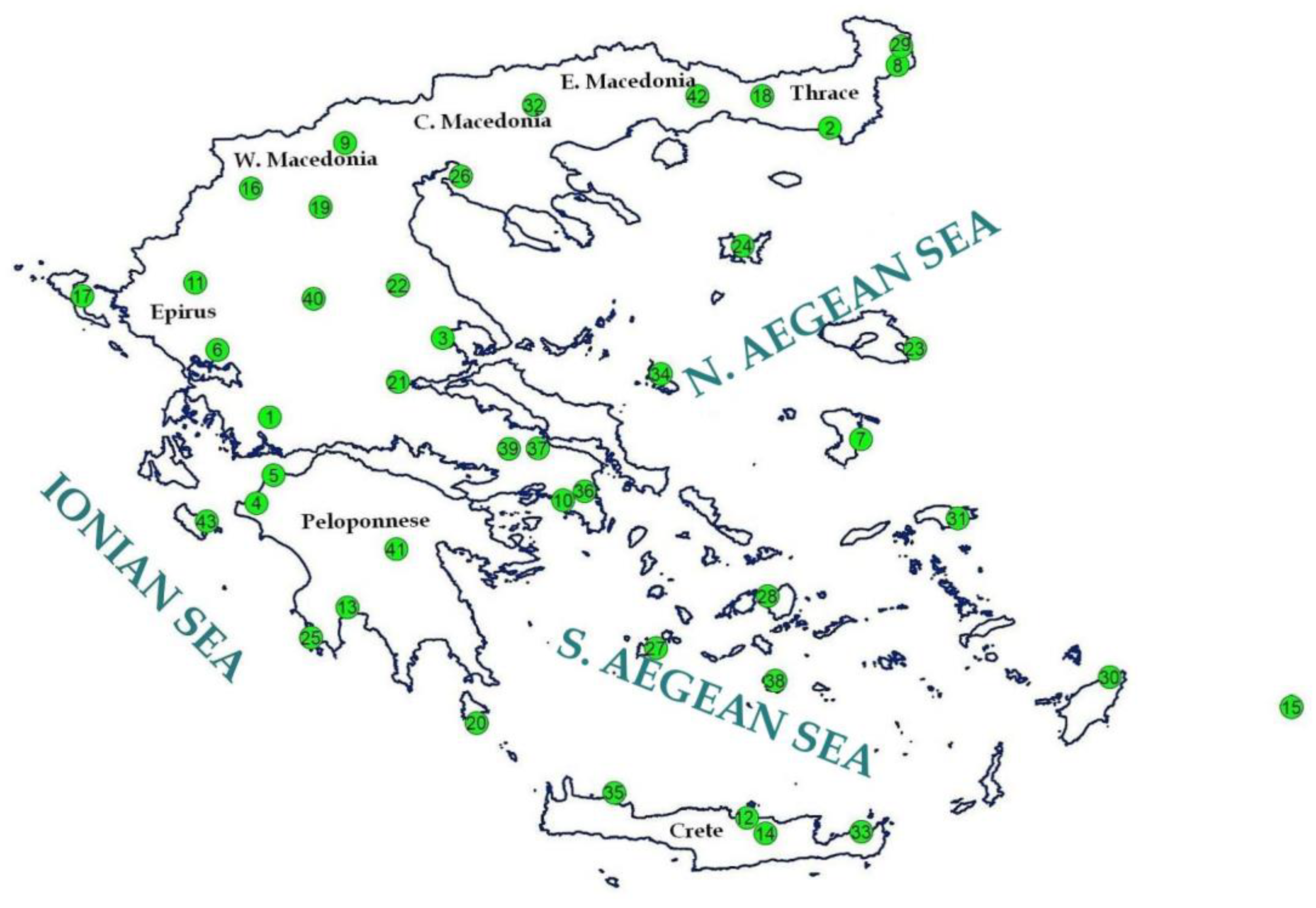
Kambezidis et al. [21] generated TMYs for 33 sites in Greece. The present study adopts these 33 sites, but 10 additional locations have been added in order to cover more efficiently the area of Greece. Table 1 shows all 43 sites (names and geographical coordinates), while Figure 1 depicts them on the map of Greece. For compatibility purposes the TMYs generated for the 33 sites in [21] have not been used here; TMYs for the 43 sites were downloaded from the PV-Geographical Information System (PV-GIS) tool instead [22], using the latest 2007–2016 Surface Solar Radiation Data Set—Heliostat (SARAH) database [23,24]. Nevertheless, it must be noted here that the TMYs thus derived would be more representative if they would have been generated from a reference period longer than 10 years (as is the period 2007–2016) in view of a changing climate worldwide. This is why the World Meteorological Organisation (WMO) recommends that a 30-year period should be used, if possible, for climatic analyses. However, it is believed that the results of this study will not be differentiated much if a period other than the one adopted would be chosen. This is supported by the fact that the qualitative characteristics of the solar radiation climate of Greece would be retained; the absolute values would only be altered.
The PV-GIS database for each of the 43 sites consists, among others, of columns referring to the year, month, day, hour UTC (universal time coordinated), global horizontal irradiance, Hg (in Wm−2), and diffuse horizontal irradiance, Hd (in Wm−2). The UTC hours were converted to LST (local standard time) = UTC + 2 h. Hourly values of kd were calculated from hourly values of the ratio Hd/Hg. Hourly values of Hb (in Wm−2) were estimated from the expression Hb = Hg − Hd. Hourly values of kb were obtained from hourly values of the ratio Hb/Hg.
Kambezidis et al. [27] derived a mathematical methodology for determining the upper and lower kd limits that classify the sky into clear, intermediate and overcast. The methodology was applied to 14 sites around the world. The main result of that work was that universal upper, kdu, and lower, kdl, limits may be used, i.e., 0.78 and 0.26, respectively. Therefore, values of kd in the ranges 0 < kd ≤ kdl = 0.26 and 0 < kd ≤ 1 were considered in the present study as they correspond to clear- and all-sky conditions, respectively. Seasonal mean and monthly mean Hg, Hd, kd, and kb values were estimated.
3. Results
3.1. Annual Mean Values
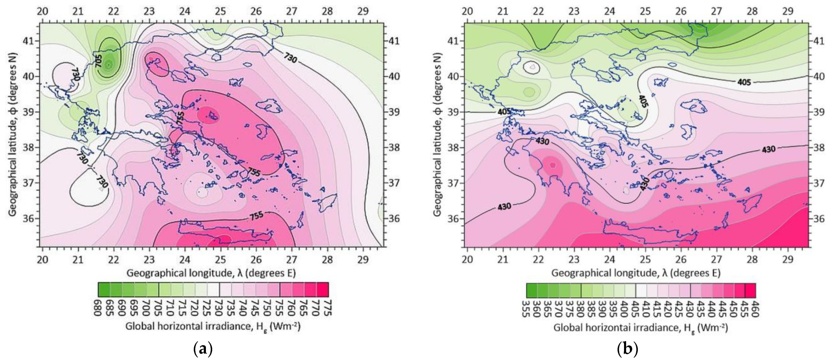
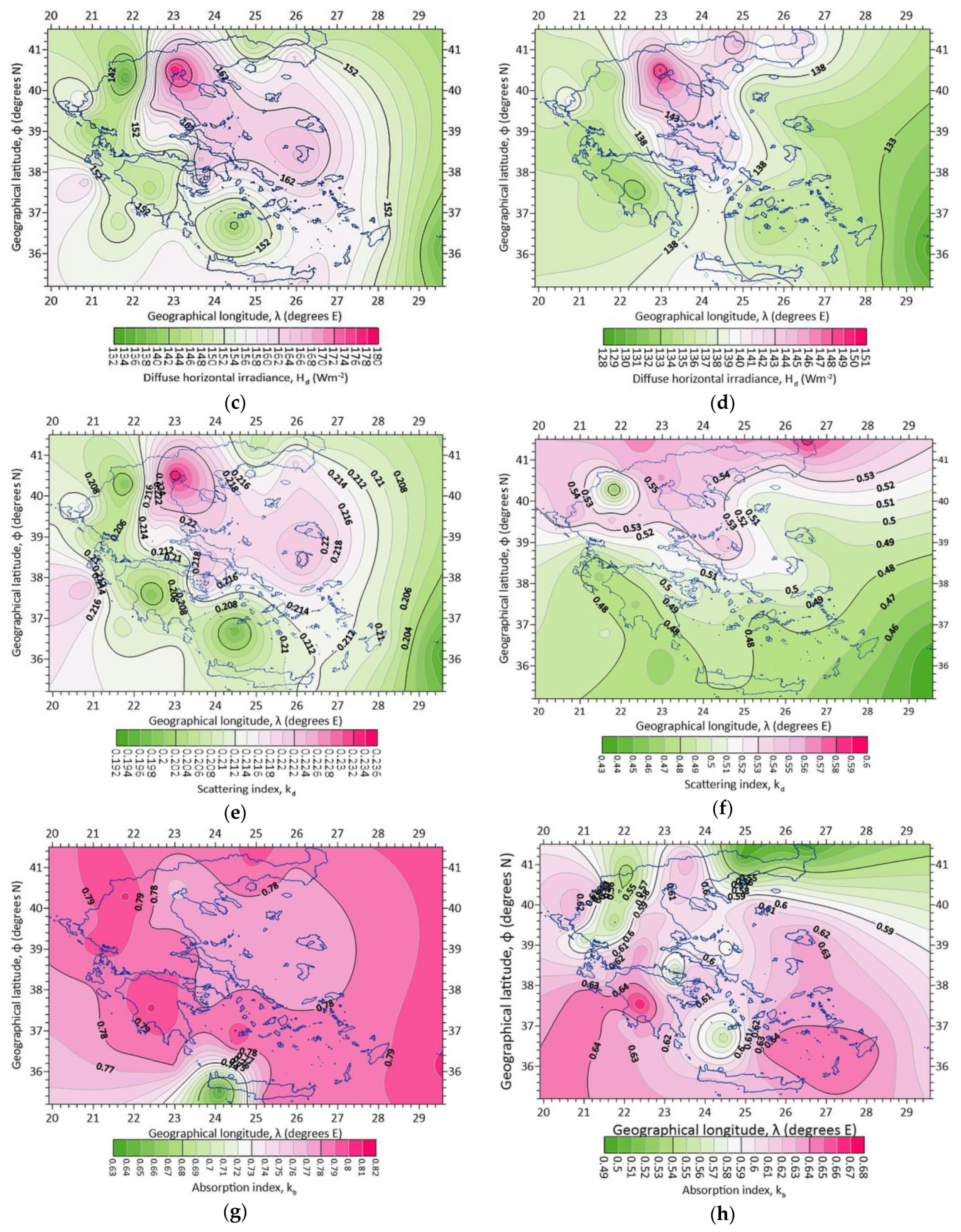
Figure 2 shows the distribution of Hg, Hd, kd, and kb for clear- (Figure 2a,c,e,g) and all- (Figure 2b,d,f,h) sky conditions over Greece. Interesting features appear and are commented upon below.
Under clear skies (Figure 2a), higher Hg values (i.e., ≈755 Wm−2) occur in northern Greece (Thessaloniki area), over most of the Aegean and all over Crete. On the contrary, lower Hg values (i.e., ≈705–730 Wm−2) exist over northwestern Greece (Epirus and most parts of western Macedonia). These observations lead to the conclusion that the total extinction of solar radiation by atmospheric constituents (both natural and additive aerosols such as desert dust, forest fires, and volcanic emissions) is at a minimum over the Aegean region and Crete. This is, of course, a coarse conclusion as one has to take into account the topography and the climatology of each of the 43 sites in the estimation of the solar radiation reaching the ground. Nevertheless, though the altitude of a site plays dominant role in the attenuation level of solar radiation, no clear conclusion seems to be extracted from Figure 3 as regards the 43 sites. Moreover, it is seen that there is great variation in the Hg levels (i.e., ≈662–702 Wm−2) even near the ground level. This may be attributed to both the latitudinal differences among these sites with z < 25 m and to the variable atmospheric turbidity levels over Greece, as depicted in Figures 12 and 13 of [17]. On the other hand, similar Hg levels appear at higher altitudes in comparison to those close to the ground. Figure 3 depicts the influence of both the topography (altitude, terrain) and climatology (geographical latitude) of the sites on solar radiation. In relation to the attenuation of the solar radiation due to the scattering mechanism, Figure 2c shows that this mechanism is stronger over the Aegean Sea (i.e., ≈162 Wm−2) and weaker over the Ionian Sea and western Greece (Epirus, Peloponnese, i.e., ≈140 Wm−2). In Figure 2e the distribution of kd over Greece is shown; it is seen that the kd pattern resembles that of Hd and it is, therefore, dominated by it. This means that the clear-sky scattering mechanism is dominant over the absorption one over the Aegean and Thessaloniki area, a conclusion that may be interpreted as the near absence of absorbing substances over these regions. Indeed, the winds in the eastern part of Greece dominate in the NE–SW direction and are generally stronger than those in the western part, thus providing a cleansing effect over the Aegean [28,29,30]. From the distribution of the absorption index over Greece shown in Figure 2g, it is found that kb dominates over kd under clear skies.
Kambezidis and Psiloglou [17] studied the atmospheric turbidity over Greece by using the Linke turbidity factor, TL, and the Unsworth–Monteith turbidity coefficient, TUM. They prepared maps of annual mean TL (their Figure 12) and TUM (their Figure 13) values for clear- and all-sky conditions, analogous to Figure 2a,b of the present work. Their distinction of clear skies was made by using the modified clearness index, k’t [31], in the range 0.65 < k’t ≤ 1, instead of kd as in the present work. Another difference is the use of the 33 TMYs derived in [21], while the present study used the PV-GIS TMYs. Therefore, a difference may be found in comparing the Hg-clear-sky map with the TL-clear-sky (TUM-clear-sky) map. Indeed, TL and TUM show higher values over the southern Ionian Sea and northern Aegean Sea, while Hg presents higher values over the Aegean and Crete regions. On the contrary, there is a better agreement between the Hd-clear-sky map (Figure 2c) with the TL and TUM ones. Higher (lower) values of Hd (TL, TUM) are found over the northern Aegean Sea, and lower (higher) values are found over most of the remaining territory of Greece. This agreement is reasonable, as the Hd solar component clearly addresses the turbidity issue (likewise the TL and TUM factors) in terms of scattering.
Under all-sky conditions, the Hg pattern (Figure 2b) seems to be much simpler than that for clear skies; the Greek territory is now split into two halves, one in the north and another in the south, with a dividing line at the geographical latitude of about 39° N. This is quite logical, as northern Greece has more cloudiness during the year than the southern part; similar results have been obtained in ([32], Figure 5a) and in ([33], Figure 1i). Cloudiness also dominates the kd pattern, as expected (Figure 2f, present work), and largely resembles that of Hg. The Hd pattern is similar to that for clear skies; in the case of cloudiness, the maximum over the Aegean is constrained to the northern part of the country (Figure 2d). As far as the absorption index is concerned (Figure 2h), this shows an exactly opposite pattern to that of kd in Figure 2f. It is notable to observe that the dividing line between these two distinct patterns is again the geographical latitude of 39° N.
In terms of the TL and TUM values from [17], the Hg pattern is now compatible with that for the two turbidity factors, because in the case of all skies there is no preference in the kd (k’t in [17]) values used. Therefore, the main outcome of this section is the right choice of the atmospheric index; kd (or k’d, similar to k’t) refers to the scattering mechanism and kb to the absorption effect, while the clearness index, kt (or k’t), refers to the total (absorption and scattering) extinction of the solar rays.
3.2. Monthly Mean Values
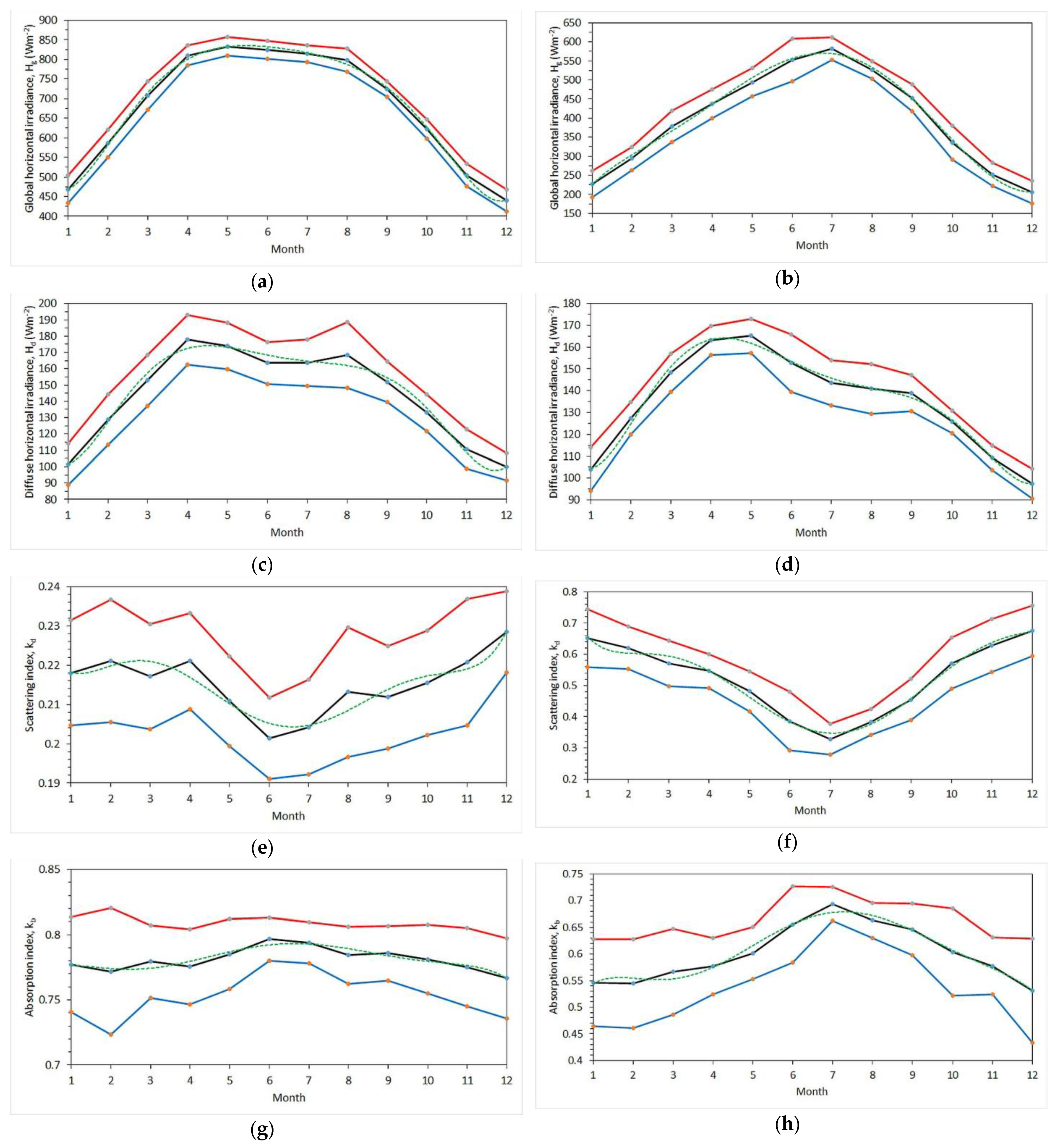
Figure 4 shows the intra-annual distribution of Hg, Hd, kd, and kb for clear- (Figure 4a,c,e,g) and all- (Figure 4b,d,f,h) sky conditions over Greece.
Under clear skies, Hg presents a rather broad maximum during the months of May–July. Since the monthly Hg values are averages over all sites, the graph in Figure 4a shows the mean situation over Greece. The broad maximum in the mentioned months may, therefore, be attributed to the (northeasterly) Etesian winds (etesian = annual) that blow every year over the Aegean from May through all summer. It seems that this natural phenomenon is dominant as a cleansing weather system in the eastern part of Greece. Indeed, Figure 2a verifies this (i.e., the high annual Hg values, ≈850 Wm−2) over the Aegean. In the case of Hd (Figure 4c), this parameter presents two main maxima, one in April (178 Wm−2) and another in August (168 Wm−2). The two maxima in the figure are in complete agreement with the higher atmospheric turbidity over Greece in these two months (see Figure 10—lower right for TL and Figure 11—lower right for TUM, both in [17]). As far as kd is concerned, Figure 4e shows that this parameter experiences lower values during summer (≈0.21), meaning a minimum contribution of the scattering particles to the total extinction of the solar rays in the Earth’s atmosphere. Indeed, a minimum scattering effect on solar radiation in the summer has been confirmed by other researchers, too. Adamopoulos et al. [34] have estimated a minimum Ångström exponent, α, in the VIS spectrum over Athens equal to 0.69, a value that implies coarser (and more scattering) particles than in the other three seasons. Additionally, Dumka et al. [35] reported a mean value of 0.55 for the scattering Ångström exponent, SAE, over the central Indian Himalayas in the same season. SAE values lower than 1 characterise large scattering particles [36]. As far as kb is concerned for Greece, rather constant values dominate all over the year with a slight maximum in summer (June, July, Figure 4g, ≈0.79). This confirms the kb pattern in Figure 2g.
Under all-sky conditions, Hg (Figure 4b) presents the expected variation of solar radiation with higher values in the summer (here in July, 582 Wm−2). The diffuse solar radiation, though, obtains higher values in springtime (April, May, Figure 4d, ≈165 Wm−2) due to the commencement of desert-dust arrival from northern Africa over Greece, mixed with scattered clouds present in this season; in addition, higher Hd levels are found in late summer (September, ≈139 Wm−2) because of the presence of desert-dust episodes that are more frequent in spring and extended summer [37]. The intra-annual variation of kd (Figure 4f) shows a clear minimum in the summer (June, July, ≈0.38) because of much lower cloudiness in the sky of Greece in comparison with that in the other three seasons. On the contrary, the kb index shows an exactly opposite behavior (July, Figure 4h, ≈0.69) to kd, in agreement with the abovementioned behaviour of these two indices.
Figure 4 shows the monthly mean values (black lines) together with the ±95% confidence interval (red and blue lines). The green dotted lines are graphical representation of the regression equations in Table 2 that fit the mean curves best. It is worth observing that all regression lines lie within the ±95% confidence band. R2 is very close to 1 in almost all cases, except for the clear-sky cases of the kd and kb indices. This at-first-glance awkward result occurs because of the great variation of the scattering and absorption mechanisms on clear-sky days. In such situations atmospheric turbulence varies remarkably over space and time (see the complicated patterns in the month–hour Linke- and Unsworth–Monteith turbidity parameter graphs in Figures 6 and 7, respectively, both in [17]). This variability is due to the absence of rain, which is catalytic in the wash-out and removal mechanisms of atmospheric aerosols in the atmosphere.
3.3. Seasonal Mean Values
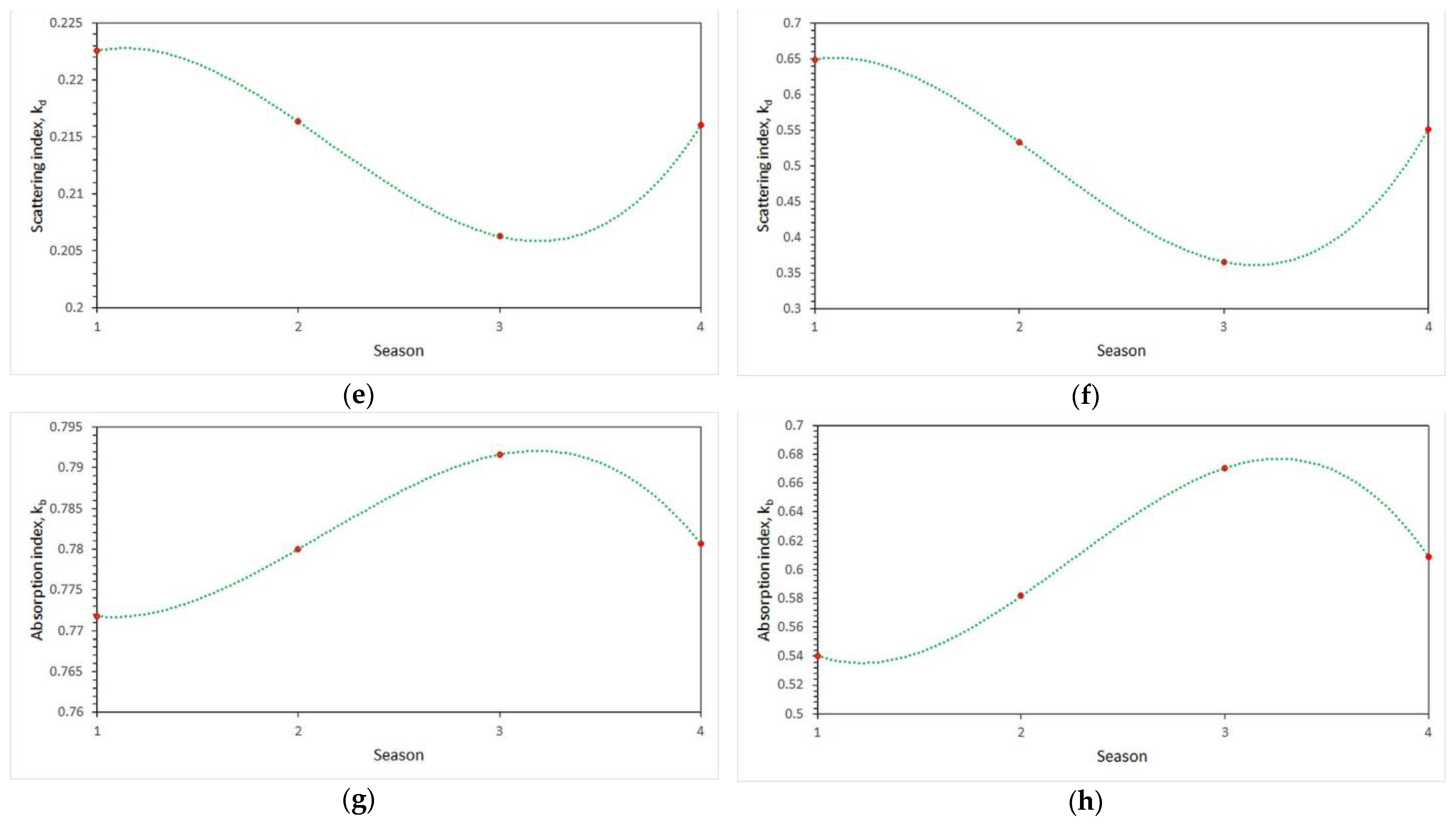
Figure 5 shows the seasonal variation of Hg, Hd, kd, and kb for clear- (Figure 5a,c,e,g) and all- (Figure 5b,d,f,h) sky conditions over Greece.
Under clear skies, the average summer value of Hg ≈813 Wm−2 (Figure 5a) is slightly higher and the average summer value of Hd ≈165 Wm−2 (Figure 5c), slightly less than that of spring (≈784 Wm−2 and ≈168 Wm−2, respectively). On the contrary, the summer kd value is the lowest among all seasons (≈0.37), a finding that implies least scattering of the solar light over Greece in summertime; this gives way to high kb values in this season (≈0.79), as expected from the opposite behaviour of these two parameters.
Under all-sky conditions, the average summer Hg level is the highest among all seasons (≈554 Wm−2), as expected, while the Hd one (≈146 Wm−2) is less than that for spring (≈159 Wm−2); the latter implies a greater contribution from the scattering mechanism in the atmosphere during spring than in the summer. Indeed, this conclusion is in agreement with the higher Hd (≈159 Wm−2) and kd (≈0.53) values in the spring months (April, May, Figure 5d,f) than in the summer months (≈146 Wm−2 and ≈0.37, respectively). The absorption index shows maximum values in summer (≈0.67, Figure 5h).
For both cases of clear and all skies, third-order regression equations have been derived that best fit the seasonal mean values of Hg, Hd, kd, and kb. Their expressions are given in Table 3.
3.4. Direct Solar Radiation
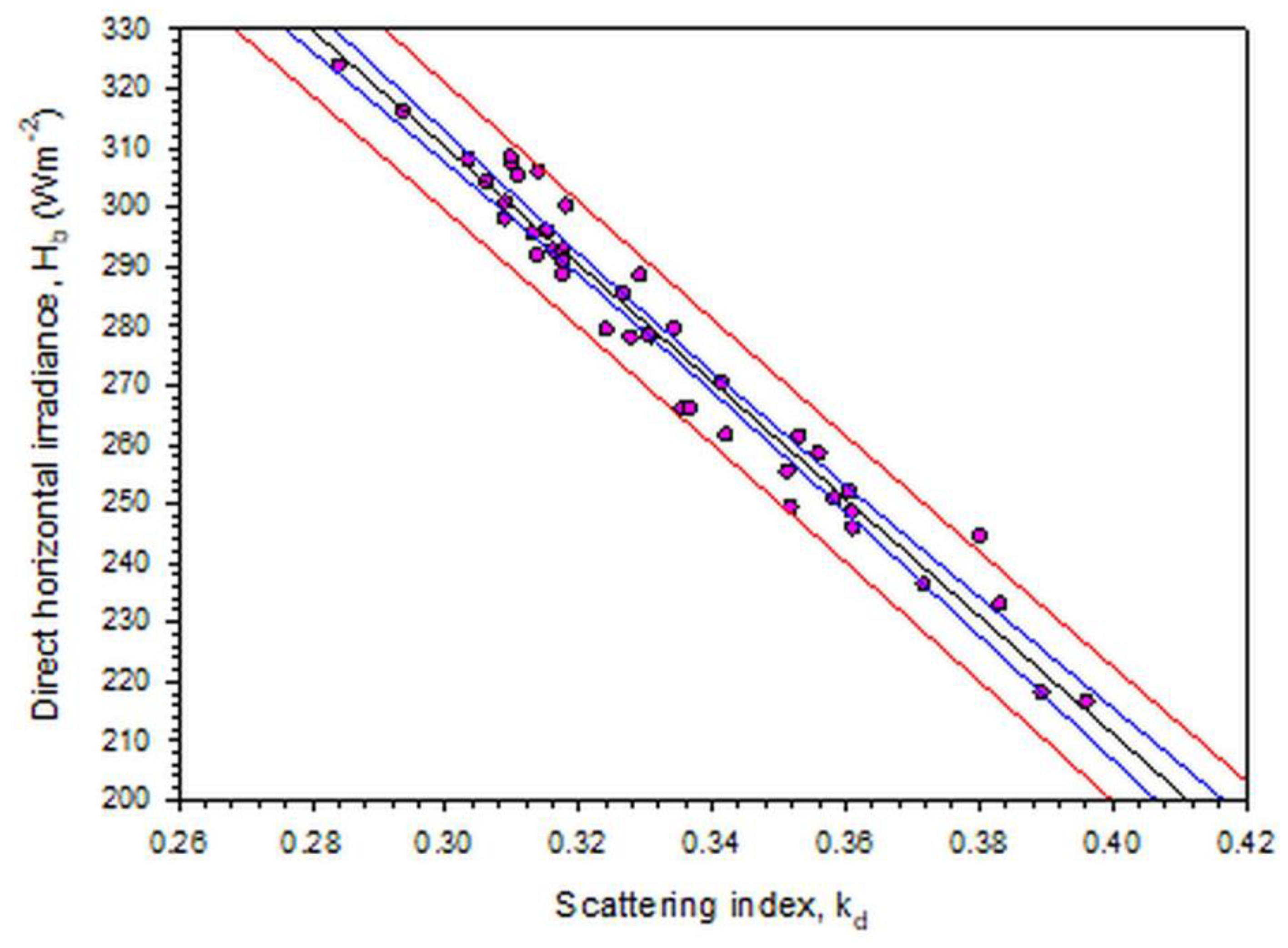
In order to find any relationship between any of the three solar radiation components with kd, graphs of their annual mean values were prepared. Scatter-plot graphs of Hg–kd, Hd–kd for both clear and all skies, and for Hb–kd under clear-sky conditions did not show any specific pattern; therefore, they are not presented here. The only meaningful pattern was for the scatter plot of Hb–kd under all-sky conditions, which is presented in Figure 6. It is interesting to observe that all sites are included in the prediction band, while very few lie within the confidence interval.
The confidence interval shows the likely range of the Hb–kd data pairs to be associated with the fitted regression line; in the 95% case it is anticipated that the regression line passes through each band (i.e., the Hb–kd value ± 1σ), and this happens for up to 95% of the data population. On the contrary, the prediction interval is related to the regression line that passes through the individual ranges of new (future) data pairs; in the 95% case this should occur for up to 95% of new (future) values. The definition of the two intervals can be applied and interpreted in the case of Figure 6 as follows. The regression line loosely represents the Hb–kd function, but it is anticipated that this regression equation will be significant (be more confident) in representing new (future) data pairs. The word “future” has the meaning of a changing global climate.
Another interesting feature from Figure 6 is the negative linear dependence of Hb on kd. If one assumes Hg to be constant in the ratio Hd/Hg, then an increase in Hd (i.e., increase in kd) results in a decrease in Hb because of the linear relationships Hg = Hd + Hb or kd = 1 − Hb/Hg (if both sides of the former equation are divided by Hg, the ratio Hd/Hg is replaced with kd, and the equation is solved for kd).
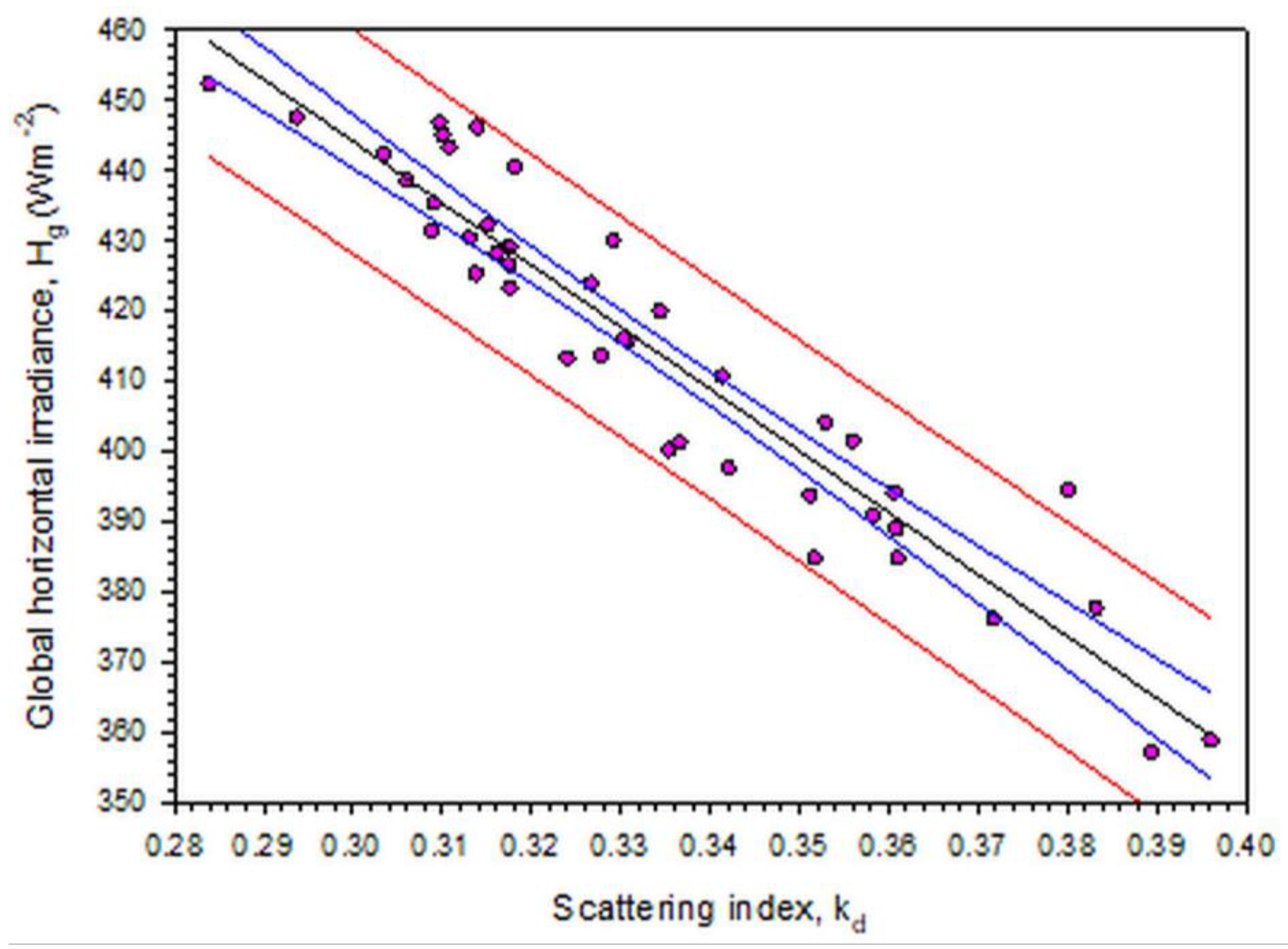
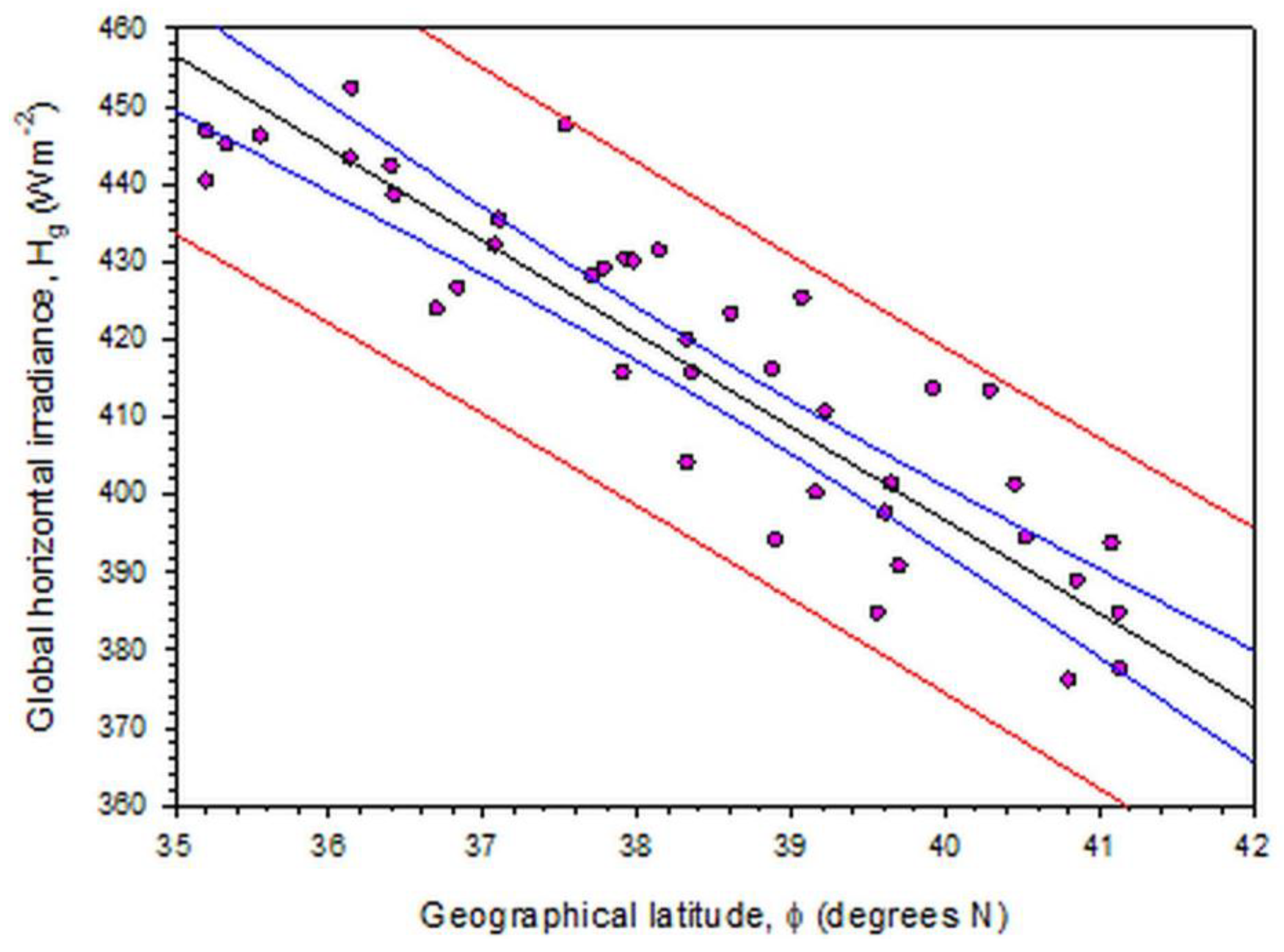
3.5. Dependence of Hg on kd or on φ
Upon investigating the dependence of Hg on kd or on φ, Figure 7 and Figure 8 were derived. Figure 7 shows a plot of the annual mean Hg values versus the annual mean kd ones, while Figure 8 presents a scatter plot of the annual mean Hg values versus φ for all 43 sites. Both scatter plots are fitted by linear regression lines from which the annual global horizontal irradiance can be estimated for a known value of kd or φ. The confidence and prediction intervals are shown and have the same meaning with those in Figure 6.
3.6. Extinction of Solar Radiation over Greece
In the previous sections the scattering process over Greece was examined in terms of the diffuse fraction (or scattering index), kd. In the same way, the absorption of solar radiation can be expressed by the direct-beam fraction (or absorption index), kb = Hb/Hg, as mentioned in Section 2. By replacing kd and kb with Hd/Hg and Hb/Hg, respectively, in the basic equation Hg = Hd + Hb, it is found that kd + kb = 1. This equation says that the scattering and absorption effects (if reflections in the atmosphere are omitted) are summed up to 1 (i.e., to the total extinction of solar rays). Figure 9 shows the annual mean values of kd, and kb over the 43 sites in Greece under clear (Figure 9a) and all (Figure 9b) skies. It is clearly seen that the absorption mechanism is always stronger over Greece than the scattering one, i.e., kb ≈ 4 kd, and kb ≈ 2 kd, under clear- and all-sky conditions, respectively.
It is quite interesting to observe that both extinction indices are constant all over Greece under clear-sky conditions. This implies a uniformity of the scattering and absorbing particles over the country. In clear weather, the extinction of solar light is due to the atmospheric constituents (omitting reflections from the ground). The extinction comes from atmospheric particles that scatter (nitrogen, oxygen, desert dust) and/or absorb (carbon dioxide, water vapour, ozone) solar light. The two attenuating mechanisms of solar radiation over Greece are depicted in Figure 9a. The dominance of absorption over scattering under clear skies indicated in Figure 2g is also confirmed in Figure 9.
Under all-sky conditions, the scatterers/absorbers seem to increase/decrease their effect with geographical latitude. This occurs because the extra particles in the atmosphere are now the clouds that scatter solar light. Therefore, as φ increases from 35° N to 42° N the probability of cloudiness (both cloud cover and clouds type) becomes higher. These causes increase the scattering of solar radiation and, thus, a decrease in absorption occurs because of the basic equation kd + kb = 1; this equation is verified if the values of kd and kb for any 32° < φ < 42° are added along the best-fit lines in Figure 9a or Figure 9b. Figure 9b depicts the two attenuating mechanisms of solar radiation over Greece for all-sky conditions.
Bai and Zong [38], in an effort to develop a solar radiation model for the location of Qianyanzhou in China to estimate Hg as a sum of absorbing and scattering losses of Hg in the atmosphere, observed that: (i) the absorbing losses (expressed by kb in the present study) were higher in spring under clear- and all-sky conditions; (ii) the scattering losses (expressed by kd in their publication and in the present work) were higher in spring and winter under clear skies (in agreement with Figure 5e of the present study) and higher in spring and summer under all skies (not compared well with Figure 5f in the present study; this disagreement may be due to variations in cloudiness during the year between Greece and China); (iii) the extinction of Hg was dominated by absorption losses in all seasons (in agreement with Figure 9 of the present study). The reason that the results in the mentioned study are not in full agreement with those of the present work is due to the different meteorological patterns occurring year-round over Greece and China. Nevertheless, the fact that some of these results were found to agree between each other provides a basic background for the similar behaviour of the scattering and absorption mechanisms worldwide.
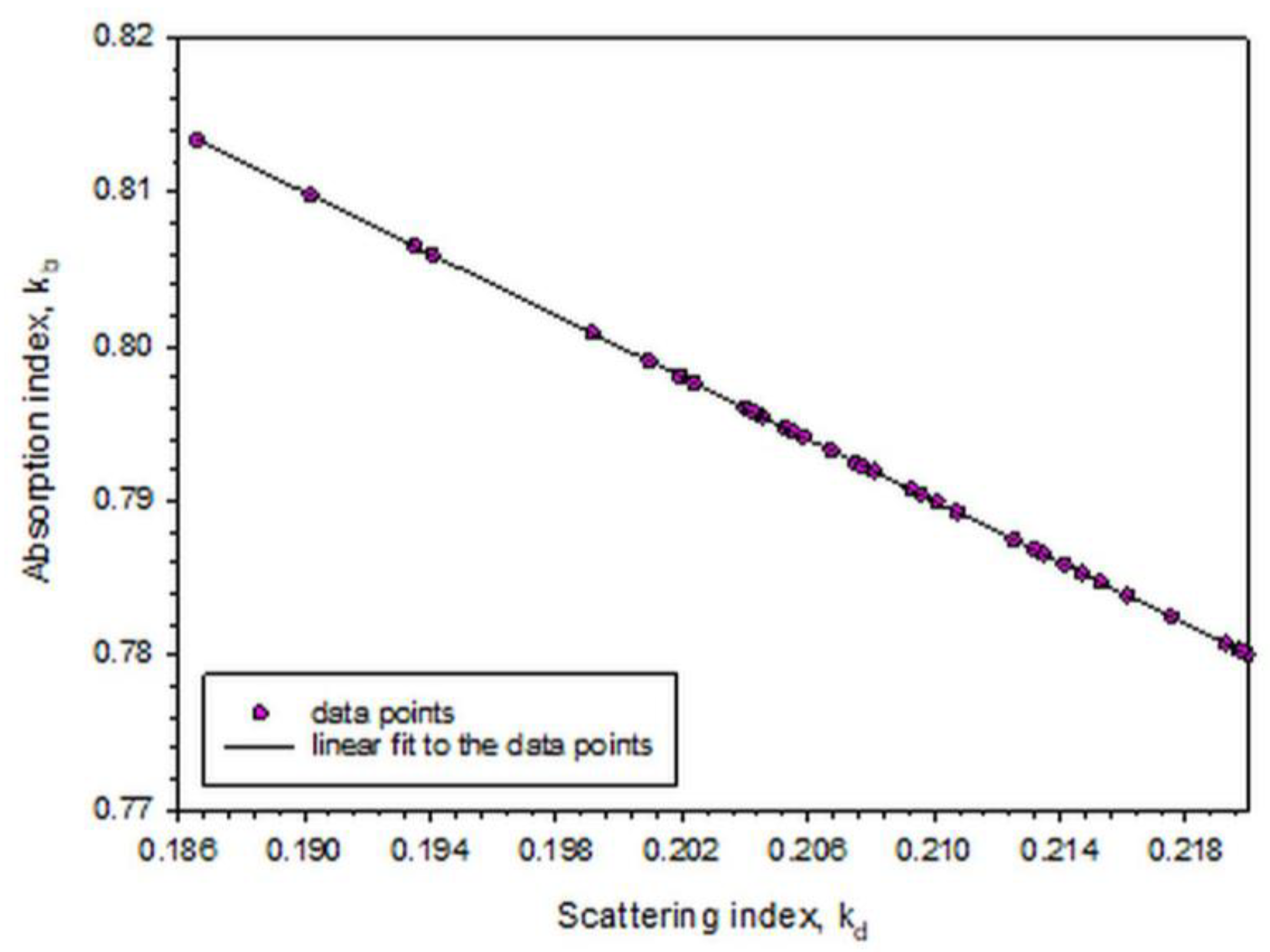
Figure 10 shows the linear relationship between kb and kd under all-sky conditions. It is observed that the equation of the fitted line verifies the basic equation kb + kd = 1.
3.7. Solar Variability and Solar Radiation over Athens
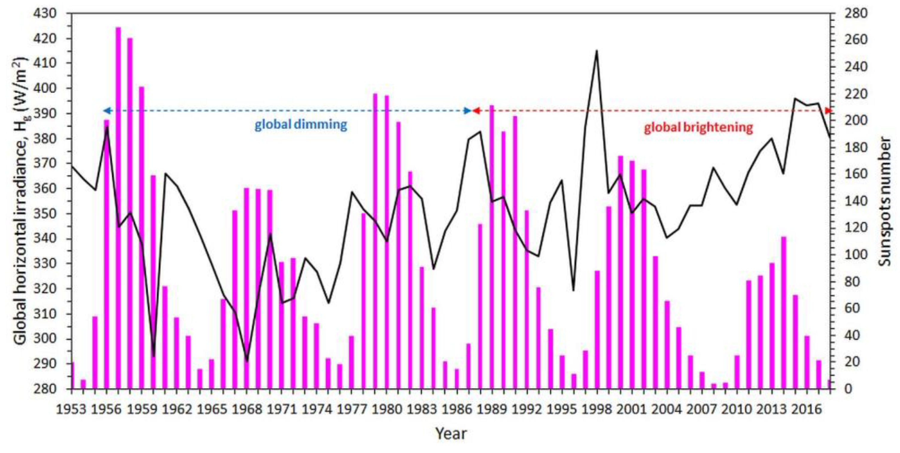
The National Observatory of Athens operates a unique and complete solar platform (the Actinometric Station of the National Observatory of Athens, ASNOA; 37.97° N, 22.72° E, 107 m asl). Figure 11 shows the variation of the annual mean Hg values from the ASNOA records in the period 1953–2018. The yearly sunspot numbers have also been added in the graph for comparison with solar radiation. The periods of the global dimming and global brightening effects over the Athens area [5,39,40,41] are also indicated. Interesting pieces of information can be extracted from the graph: (i) the solar radiation recorded at ASNOA does not follow exactly the solar activity (sunspots cycle); (ii) the peaks of solar activity (highest sunspot numbers) do not necessarily coincide with the peaks in solar radiation; (iii) solar radiation has been recently increasing, though the solar activity after 2007 (solar cycle 24) is very low (quiet Sun); (iv) the absence of co-variance between the two data series shows that solar activity has a less significant effect on solar radiation reaching the surface of the Earth in comparison with the effect exerted by atmospheric aerosols. Indeed, the global dimming effect has been attributed to an increase in anthropogenic (air pollution) aerosols mainly over big cities and large industrial estates [42,43,44].
4. Discussion
The present work studied the solar radiation climate of Greece. That was done through adopting typical meteorological years for 43 sites in Greece. The use of TMYs in various applications is attracting more and more attention by scientists/users because each TMY contains robust information for the climate at a location; see, e.g., [21,45,46,47]. The use of TMYs is also attracting attention in solar radiation applications; see, e.g., [48,49,50,51].
The present work was the first for Greece in studying the solar radiation climate of the country and among few in the international literature. The knowledge of the solar climate of a region or a country is precious as it dictates the solar availability, i.e., the solar radiation levels expected, and, to a certain extent, it elucidates the climate of the area, because solar radiation is one of the most important parameters comprising local climate. The analysis in the present study was focused on the three solar radiation components based on the TMYs of 43 sites in Greece. Use of the diffuse fraction, kd, (or else cloudiness index [52]), and the absorption index, kb, was made. As far as the latter index is concerned, this was the first time that it was introduced in the literature to the author’s best knowledge.
The diffuse fraction (the scattering index) shows the weight of the diffusively scattered solar radiation by atmospheric molecules (in clear-sky conditions) and by atmospheric aerosols and clouds combined (under all-sky conditions) over the received global solar radiation on the surface of the Earth; in other words, kd reflects the attenuation of solar radiation by scattering in the atmosphere. The direct-beam fraction (the absorption index) shows the weight of the attenuated (absorbed) direct solar radiation by atmospheric molecules (under clear skies) or attenuated (absorbed and scattered) by atmospheric aerosols and clouds (under all skies) to the received global solar irradiance on the surface of the Earth. The present study speculated that kb represents more the absorption of solar radiation than the scattering effect. The assumption proved to be true from solar radiation measurements, as demonstrated in Figure 9 and Figure 10.
From the above, it is concluded that the kd and kb indices (and especially the kb one introduced in the present work) can from now on be used in studies describing the atmospheric scattering and absorption mechanisms, respectively. This conclusion becomes robust because of the evaluation of the basic equation kb + kd = 1.
5. Conclusions
In view of the above, the following conclusions can be summarised.
- Under clear skies, higher annual Hg values occur in northern Greece (Thessaloniki area), over most of the Aegean and all over Crete. On the contrary, lower annual Hg values exist over northwestern Greece (Epirus and most parts of western Macedonia). The annual kd pattern resembles that of Hd. High values of kb dominate almost all over Greece.
- Under all-sky conditions, the annual Hg pattern is split into two halves, one in the north and another in the south with a dividing line at the latitude of about 39° N. The distribution of the annual Hd levels is similar to that for clear skies. The annual kd pattern resembles much that of Hg, while that for kb is quite the opposite.
- Under clear skies, the intra-annual Hg levels present a rather broad maximum during the months of May–July. In the case of Hd, this parameter presents two main maxima, one in April and another in August. As far as kd is concerned, this parameter experiences lower values during the summer. The absorption index shows a rather flat behaviour throughout the year.
- Under all-sky conditions, the monthly mean Hg values are higher in the summer (here in July). The diffuse solar radiation, though, obtains higher values in springtime (April, May). The intra-annual variation of kd shows a clear minimum in the summer (June, July), whereas kb obtains maximum values in the summer.
- Under clear skies, the average summer value of Hg is slightly higher and the average summer value of Hd slightly lower than that of spring. The average summer value of kd is the lowest among all seasons, while that for kb is the highest. The same conclusions apply in the case of all skies.
- Under all skies, Hg decreases with increasing kd; the same behaviour exists for increasing φ.
- The kd and kb indices reflect the scattering and absorption mechanisms of solar radiation in the atmosphere. The expression kd + kb = 1 was validated.
- kd increases and kb decreases with increasing φ under all-sky conditions.
Funding
This research received no external funding.
Institutional Review Board Statement
Not applicable.
Data Availability Statement
The solar radiation data for the 43 sites in Greece were downloaded from the freeware PV-GIS platform at https://ec.europa.eu/jrc/en/pvgis, and the sunspot numbers from the site of the Royal Observatory of Belgium at https://wwwbis.sidc.be/silso/infosnytot (both websites accessed on 10 October 2021). The ASNOA solar radiation data are available upon request, but they were used on a self-evident permission to the author as ex. member and now Emeritus Researcher in the Institution.
Acknowledgments
The author thanks the personnel of the PV–GIS platform for providing the necessary solar horizontal irradiances over Greece. He also acknowledges N. Kappos for maintaining the solar radiation equipment on the ASNOA platform, and F. Pierros for quality checking and archiving the solar radiation data.
Conflicts of Interest
The authors declare no conflict of interest.
References
- Giesen, R.H.; van den Broeke, M.R.; Oerlemans, J.; Andreassen, L.M. Surface energy balance in the ablation zone of Midtdalsbreen, a glacier in Southern Norway: Interannual variability and the effect of clouds. J. Geophys. Res. 2008, 113, D21111. [Google Scholar] [CrossRef]
- Asaf, D.; Rotenberg, E.; Tatarinov, F.; Dicken, U.; Montzka, S.A.; Yakir, D. Ecosystem photosynthesis inferred from measurements of carbonyl sulphide flux. Nat. Geosci. 2013, 6, 186–190. [Google Scholar] [CrossRef]
- Bojinski, S.; Verstraete, M.; Peterson, T.C.; Richter, C.; Simmons, A.; Zemp, M. The concept of essential climate variables in support of climate research, applications, and policy. Bull. Am. Meteorol. Soc. 2014, 95, 1431–1443. [Google Scholar] [CrossRef]
- Kambezidis, H.D. The solar resource. In Comprehensive Renewable Energy; Elsevier: Amsterdam, The Netherlands, 2012; Volume 3. [Google Scholar] [CrossRef]
- Kambezidis, H.D. The solar radiation climate of athens: Variations and tendencies in the period 1992–2017, the Brightening Era. Sol. Energy 2018, 173, 328–347. [Google Scholar] [CrossRef]
- Forster, P.M. Inference of climate sensitivity from analysis of earth’s energy budget. Annu. Rev. Earth Planet. Sci. 2016, 44, 85–106. [Google Scholar] [CrossRef]
- Haywood, J.; Boucher, O. Estimates of the direct and indirect radiative forcing due to tropospheric aerosols: A review. Rev. Geophys. 2000, 38, 513–543. [Google Scholar] [CrossRef]
- Puetz, S.J.; Prokoph, A.; Borchardt, G. Evaluating alternatives to the milankovitch theory. J. Stat. Plan. Inference 2016, 170, 158–165. [Google Scholar] [CrossRef] [Green Version]
- Madhlopa, A. Solar radiation climate in malawi. Sol. Energy 2006, 80, 1055–1057. [Google Scholar] [CrossRef]
- Jiménez, J.I. Solar radiation statistic in Barcelona, Spain. Sol. Energy 1981, 27, 271–282. [Google Scholar] [CrossRef]
- Dissing, D.; Wendler, G. Solar radiation climatology of Alaska. Theor. Appl. Climatol. 1998, 61, 161–175. [Google Scholar] [CrossRef]
- Petrenz, N.; Sommer, M.; Berger, F.H. Long-time global radiation for Central Europe derived from ISCCP Dx data. Atmos. Chem. Phys. 2007, 7, 5021–5032. [Google Scholar] [CrossRef] [Green Version]
- Nottrott, A.; Kleissl, J. Validation of the NSRDB-SUNY global horizontal irradiance in California. Sol. Energy 2010, 84, 1816–1827. [Google Scholar] [CrossRef]
- Persson, T. Solar radiation climate in Sweden. Phys. Chem. Earth 1999, 24, 275–279. [Google Scholar] [CrossRef]
- Exell, R.H.B. The solar radiation climate of Thailand. Sol. Energy 1976, 18, 349–354. [Google Scholar] [CrossRef]
- Diabaté, L.; Blanc, P.; Wald, L. Solar radiation climate in Africa. Sol. Energy 2004, 76, 733–744. [Google Scholar] [CrossRef] [Green Version]
- Kambezidis, H.D.; Psiloglou, B.E. Climatology of the Linke and Unsworth-Monteith turbidity parameters for Greece: Introduction to the notion of a typical atmospheric turbidity year. Appl. Sci. 2020, 10, 4043. [Google Scholar] [CrossRef]
- Unsworth, M.H.; Monteith, J.L. Aerosol and solar radiation in Britain. Q. J. R. Meteorol. Soc. 1972, 98, 778–797. [Google Scholar] [CrossRef]
- Kambezidis, H.D.; Adamopoulos, A.D.; Zevgolis, D. Determination of Ångström and Schüepp’s parameters from ground-based spectral measurements of beam irradiance in the ultraviolet and visible spectrum in Athens, Greece. Pure Appl. Geophys. 2001, 158, 821–838. [Google Scholar] [CrossRef]
- Janjai, S.; Kumharn, W.; Laksanaboonsong, J. Determination of angstrom’s turbidity coefficient over Thailand. Renew. Energy 2003, 28, 1685–1700. [Google Scholar] [CrossRef]
- Kambezidis, H.D.; Psiloglou, B.E.; Kaskaoutis, D.G.; Karagiannis, D.; Petrinoli, K.; Gavriil, A.; Kavadias, K. Generation of typical meteorological years for 33 locations in Greece: Adaptation to the needs of various applications. Theor. Appl. Climatol. 2020, 141, 1313–1330. [Google Scholar] [CrossRef]
- Huld, T.; Müller, R.; Gambardella, A. A new solar radiation database for estimating PV performance in Europe and Africa. Sol. Energy 2012, 86, 1803–1815. [Google Scholar] [CrossRef]
- Urraca, R.; Gracia-Amillo, A.M.; Koubli, E.; Huld, T.; Trentmann, J.; Riihelä, A.; Lindfors, A.V.; Palmer, D.; Gottschalg, R.; Antonanzas-Torres, F. Extensive validation of CM SAF surface radiation products over Europe. Remote Sens. Environ. 2017, 199, 171–186. [Google Scholar] [CrossRef] [PubMed] [Green Version]
- Urraca, R.; Huld, T.; Gracia-Amillo, A.; Martinez-de-Pison, F.J.; Kaspar, F.; Sanz-Garcia, A. Evaluation of global horizontal irradiance estimates from ERA5 and COSMO-REA6 reanalyses using ground and satellite-based data. Sol. Energy 2018, 164, 339–354. [Google Scholar] [CrossRef]
- ELOT. Information and Documentation: Conversion of Greek Characters into Latin Characters. Standard 743; Multiple. Distributed through American National Standards Institute: Washington, DC, USA, 2001; ICS 01.140.10. [Google Scholar]
- ISO. Information and Documentation: Conversion of Greek Characters into Latin Characters. Standard 843; Multiple. Distributed through American National Standards Institute: Washington, DC, USA, 1997; ICS 01.140.10. [Google Scholar]
- Kambezidis, H.D.; Kampezidou, S.I.; Kampezidou, D. Mathematical determination of the upper and lower limits of the diffuse fraction at any site. Appl. Sci. 2021, 11, 8654. [Google Scholar] [CrossRef]
- Sahsamanoglou, H.S.; Bloutsos, A.A. Cleansing of the atmosphere in the Athens area by means of rainfall and wind. Energy Build. 1982, 4, 125–128. [Google Scholar] [CrossRef]
- Adamopoulos, A.D.; Kambezidis, H.D.; Zevgolis, D. Total atmospheric transmittance in the UV and VIS spectra in Athens, Greece. Pure Appl. Geophys. 2005, 162, 409–431. [Google Scholar] [CrossRef]
- Giavis, G.M.; Kambezidis, H.D.; Lykoudis, S.P. Frequency distribution of particulate MATTER (PM10) in urban environments. Int. J. Environ. Pollut. 2009, 36, 99–109. [Google Scholar] [CrossRef]
- Perez, R.; Ineichen, P.; Seals, R.; Zelenka, A. Making full use of the clearness index for parameterizing hourly insolation conditions. Sol. Energy 1990, 45, 111–114. [Google Scholar] [CrossRef] [Green Version]
- Katopodis, T.; Markantonis, I.; Politi, N.; Vlachogiannis, D.; Sfetsos, A. High-resolution solar climate atlas for Greece under climate change using the weather research and forecasting (WRF) model. Atmosphere 2020, 11, 761. [Google Scholar] [CrossRef]
- Ioannidis, E.; Lolis, C.J.; Papadimas, C.D.; Hatzianastassiou, N.; Bartzokas, A. On the intra-annual variation of cloudiness over the Mediterranean region. Atmos. Res. 2018, 208, 246–256. [Google Scholar] [CrossRef]
- Adamopoulos, A.D.; Kambezidis, H.D.; Kaskaoutis, D.G.; Giavis, G. A study of aerosol particle sizes in the atmosphere of Athens, Greece, retrieved from solar spectral measurements. Atmos. Res. 2007, 86, 194–206. [Google Scholar] [CrossRef]
- Dumka, U.C.; Kaskaoutis, D.G.; Sagar, R.; Chen, J.; Singh, N.; Tiwari, S. First results from light scattering enhancement factor over central Indian Himalayas during GVAX campaign. Sci. Total Environ. 2017, 605–606, 124–138. [Google Scholar] [CrossRef] [PubMed]
- Schmeisser, L.; Andrews, E.; Ogren, J.A.; Sheridan, P.; Jefferson, A.; Sharma, S.; Kim, J.E.; Sherman, J.P.; Sorribas, M.; Kalapov, I.; et al. Classifying aerosol type using in situ surface spectral aerosol optical properties. Atmos. Chem. Phys. 2017, 17, 12097–12120. [Google Scholar] [CrossRef] [Green Version]
- Gkikas, A.; Hatzianastassiou, N.; Mihalopoulos, N.; Katsoulis, V.; Kazadzis, S.; Pey, J.; Querol, X.; Torres, O. The regime of intense desert dust episodes in the Mediterranean based on contemporary satellite observations and ground measurements. Atmos. Chem. Phys. 2013, 13, 12135–12154. [Google Scholar] [CrossRef] [Green Version]
- Bai, J.; Zong, X. Global solar radiation transfer and its loss in the atmosphere. Appl. Sci. 2021, 11, 2651. [Google Scholar] [CrossRef]
- Kambezidis, H.D.; Kaskaoutis, D.G.; Kharol, S.K.; Moorthy, K.K.; Satheesh, S.K.; Kalapureddy, M.C.R.; Badarinath, K.V.S.; Sharma, A.R.; Wild, M. Multi-decadal variation of the net downward shortwave radiation over South Asia: The solar dimming effect. Atmos. Environ. 2012, 50, 360–372. [Google Scholar] [CrossRef]
- Nastos, P.T.; Kambezidis, H.D.; Demetriou, D. Solar dimming/brightening within the Mediterranean. In Proceedings of the 13th International Conference on Environmental Science and Technology, Athens, Greece, 5–7 September 2013; Global NEST: Athens, Greece, 2013. ISBN 978-960-7475-51-0. [Google Scholar]
- Kambezidis, H.D.; Kaskaoutis, D.G.; Kalliampakos, G.K.; Rashki, A.; Wild, M. The solar dimming/brightening effect over the Mediterranean basin in the period 1979–2012. J. Atmos. Sol.-Terr. Phys. 2016, 150–151, 31–46. [Google Scholar] [CrossRef]
- Gilgen, H.; Wild, M.; Ohmura, A. Means and trends of shortwave irradiance at the surface estimated from global energy balance archive data. J. Clim. 1998, 11, 2042–2061. [Google Scholar] [CrossRef]
- Gilgen, H.; Roesch, A.; Wild, M.; Ohmura, A. Decadal changes in shortwave irradiance at the surface in the period from 1960 to 2000 estimated from global energy balance archive data. J. Geophys. Res. Atmos. 2009, 114. [Google Scholar] [CrossRef] [Green Version]
- Wild, M. Global dimming and brightening: A review. J. Geophys. Res. Atmos. 2009, 114. [Google Scholar] [CrossRef] [Green Version]
- Chan, A.L.S. Generation of typical meteorological years using genetic algorithm for different energy systems. Renew. Energy 2016, 90, 1–13. [Google Scholar] [CrossRef]
- Farah, S.; Saman, W.; Boland, J. Development of robust meteorological year weather data. Renew. Energy 2018, 118, 343–350. [Google Scholar] [CrossRef]
- Janjai, S.; Deeyai, P. Comparison of methods for generating typical meteorological year using meteorological data from a tropical environment. Appl. Energy 2009, 86, 528–537. [Google Scholar] [CrossRef]
- Bre, F.; e Silva Machado, R.M.; Lawrie, L.K.; Crawley, D.B.; Lamberts, R. Assessment of solar radiation data quality in typical meteorological years and its influence on the building performance simulation. Energy Build. 2021, 250, 111251. [Google Scholar] [CrossRef]
- Mosalam Shaltout, M.A.; Tadros, M.T.Y. Typical solar radiation year for egypt. Renew. Energy 1994, 4, 387–393. [Google Scholar] [CrossRef]
- Chang, K.; Zhang, Q. Improvement of the hourly global solar model and solar radiation for air-conditioning design in China. Renew. Energy 2019, 138, 1232–1238. [Google Scholar] [CrossRef]
- Huang, K.T. Identifying a suitable hourly solar diffuse fraction model to generate the typical meteorological year for building energy simulation application. Renew. Energy 2020, 157, 1102–1115. [Google Scholar] [CrossRef]
- Soneye, O.O. Evaluation of clearness index and cloudiness index using measured global solar radiation data: A case study for a tropical climatic region of Nigeria. Atmosfera 2021, 34, 25–39. [Google Scholar] [CrossRef]
Figure 1.
Distribution of the 43 sites across Greece. The numbers refer to those in column 1, Table 1. N. = North; S. = South; C. = Central; W. = West; E. = East.
Figure 1.
Distribution of the 43 sites across Greece. The numbers refer to those in column 1, Table 1. N. = North; S. = South; C. = Central; W. = West; E. = East.

Figure 2.
Mean annual (a) Hg, (c) Hd, (e) kd, and (g) kb values for clear-, and annual mean (b) Hg, (d) Hd, (f) kd, and (h) kb values for all-sky conditions over Greece.
Figure 2.
Mean annual (a) Hg, (c) Hd, (e) kd, and (g) kb values for clear-, and annual mean (b) Hg, (d) Hd, (f) kd, and (h) kb values for all-sky conditions over Greece.


Figure 3.
Variation of the annual mean Hg values at the 43 sites under clear-sky conditions as a function of their altitude, z (in m asl; asl = above sea level). It is interesting to observe the great variation in the Hg values (between ≈662 and ≈702 Wm−2) at sites with altitude even lower than 25 m asl (to the left of the vertical black dashed line).

Figure 4.
Monthly mean (a) Hg, (c) Hd, (e) kd, and (g) kb values under clear-, and monthly mean (b) Hg, (d) Hd, (f) kd, and (h) kb values under all-sky conditions over Greece. The values are averages over all 43 sites. The black lines are the means, and the red and blue curves are the mean + 1σ and mean − 1σ, respectively (σ = standard deviation), while the green dotted lines represent the best-fit curves to the mean values. The months are in sequence of January (1) to December (12).

Figure 5.
Seasonal mean (a) Hg, (c) Hd, (e) kd, and (g) kb values under clear skies, and (b) Hg, (d) Hd, (f) kd, and (h) kb values under all skies over Greece. The values are averages over all 43 sites. The green dotted lines represent the best-fit curves to the seasonal mean values. The seasons are in the sequence of winter (1) to autumn (4); winter = December, January, February; spring = March, April, May; summer = June, July, August; autumn = September, October, November.


Figure 6.
Scatter plot of the annual mean values of Hb for the 43 sites as function of their kd under all-sky conditions. The black line is a linear fit to the data points expressed by the equation Hb = −988.799·kd + 606.766 with R2 = 0.963. The blue band represents the ±95% confidence interval, and the red one the ±95% prediction interval.

Figure 7.
Scatter plot of the annual mean values of Hg for the 43 sites as function of their diffuse fraction, kd, under all-sky conditions. The black solid line is a linear fit to the data points expressed by the equation Hg = −880.811·kd + 708.462 with R2 = 0.904. The blue band represents the ±95% confidence interval, and the red one the ±95% prediction interval.

Figure 8.
Scatter plot of the annual mean values of Hg for the 43 sites as function of their geographical latitude, φ, under all-sky conditions. The black solid line is a linear fit to the data points expressed by the equation Hg = −11.968·φ + 875.431 with R2 = 0.809. The blue band represents the ±95% confidence interval, and the red one the ±95% prediction interval.

Figure 9.
Scatter plots of the annual mean values of the extinction coefficient for the 43 sites as function of their geographical latitude, φ, under (a) clear-, and (b) all-sky conditions. The horizontal blue and red dashed lines represent the average values of kd and kb, respectively. The blue and red solid lines are linear fits to the kd and kb data, respectively, expressed by the equations kd = 0.0116 φ − 0.1132 with R2 = 0.6532 and kb = −0.0116 φ + 1.1132 with R2 = 0.6532.

Figure 10.
Scatter plot of the annual mean values of kb (absorption) versus the annual mean values of kd (scattering) for the 43 sites under all-sky conditions. The black solid line is the linear fit to the data points expressed by the equation kb = −kd + 1 with R2 = 1.
Figure 10.
Scatter plot of the annual mean values of kb (absorption) versus the annual mean values of kd (scattering) for the 43 sites under all-sky conditions. The black solid line is the linear fit to the data points expressed by the equation kb = −kd + 1 with R2 = 1.

Figure 11.
Diachronic variation of the annual mean Hg values (black solid line) and the sunspot number (vertical pink bars) over Athens in the period 1953–2018. The global dimming and brightening effects are indicated by blue and red double-headed arrows, respectively. The solar radiation values come from the ASNOA records, and the sunspot numbers from the Solar Influences Data Analysis Centre, Royal Observatory of Belgium.


Table 1.
The 43 sites involved in the study. The names of the locations are given in alphabetical order. The geographical longitude, λ, and the geographical latitude, φ, are in degrees; E = East (of Greenwich meridian), N = North (hemisphere). The transliteration of the Greek names of the sites into Latin ones follows the ELOT 743 standard [25], which is an adaption of the ISO 843 one [26].
| Site # | Site Name/Region/Altitude above Sea Level (m) | λ (° E) | φ (° N) |
|---|---|---|---|
| 1 | Agrinio/Western Greece/25 | 21.383 | 38.617 |
| 2 | Alexandroupoli/Eastern Macedonia and Thrace/3.5 | 25.933 | 40.850 |
| 3 | Anchialos/Thessaly/15.3 | 22.800 | 39.067 |
| 4 | Andravida/Western Greece/15.1 | 21.283 | 37.917 |
| 5 | Araxos/Western Greece/11.7 | 21.417 | 38.133 |
| 6 | Arta/Epirus/96 | 20.988 | 39.158 |
| 7 | Chios/Northern Aegean/4 | 26.150 | 38.350 |
| 8 | Didymoteicho/Eastern Macedonia and Thrace/27 | 26.496 | 41.348 |
| 9 | Edessa/Western Macedonia/321 | 22.044 | 40.802 |
| 10 | Elliniko/Attica/15 | 23.750 | 37.900 |
| 11 | Ioannina/Epirus/484 | 20.817 | 39.700 |
| 12 | Irakleio/Crete/39.3 (also written as Heraklion) | 25.183 | 35.333 |
| 13 | Kalamata/Peloponnese/11.1 | 22.000 | 37.067 |
| 14 | Kastelli/Crete/335 | 25.333 | 35.120 |
| 15 | Kastelorizo/Southern Aegean/134 | 29.576 | 36.142 |
| 16 | Kastoria/Western Macedonia/660.9 | 21.283 | 40.450 |
| 17 | Kerkyra/Ionian Islands/4 (also known as Corfu) | 19.917 | 39.617 |
| 18 | Komotini/Eastern Macedonia and Thrace/44 | 25.407 | 41.122 |
| 19 | Kozani/Western Macedonia/625 | 21.783 | 40.283 |
| 20 | Kythira/Attica/166.8 | 23.017 | 36.133 |
| 21 | Lamia/Sterea Ellada/17.4 | 22.400 | 38.850 |
| 22 | Larisa/Thessaly/73.6 | 22.450 | 39.650 |
| 23 | Lesvos/Northern Aegean/4.8 | 26.600 | 39.067 |
| 24 | Limnos/Northern Aegean/4.6 | 25.233 | 39.917 |
| 25 | Methoni/Peloponnese/52.4 | 21.700 | 36.833 |
| 26 | Mikra/Central Macedonia/4.8 | 22.967 | 40.517 |
| 27 | Milos/Southern Aegean/5 | 24.475 | 36.697 |
| 28 | Naxos/Southern Aegean/9.8 | 25.533 | 37.100 |
| 29 | Orestiada/Eastern Macedonia and Thrace/41 | 26.531 | 41.501 |
| 30 | Rodos/Southern Aegean/11.5 (also written as Rhodes) | 28.117 | 36.400 |
| 31 | Samos/Northern Aegean/7.3 | 26.917 | 37.700 |
| 32 | Serres/Central Macedonia/34.5 | 23.567 | 41.083 |
| 33 | Siteia/Crete/115.6 | 26.100 | 35.120 |
| 34 | Skyros/Sterea Ellada/17.9 | 24.550 | 38.900 |
| 35 | Souda/Crete/140 | 21.117 | 35.550 |
| 36 | Spata/Attica/67 | 23.917 | 37.967 |
| 37 | Tanagra/Sterea Ellada/139 | 23.550 | 38.317 |
| 38 | Thira/Southern Aegean/36.5 | 25.433 | 36.417 |
| 39 | Thiva/Sterea Ellada/189 | 23.320 | 38.322 |
| 40 | Trikala/Thessaly/114 | 21.768 | 39.556 |
| 41 | Tripoli/Peloponnese/652 | 22.400 | 37.533 |
| 42 | Xanthi/Eastern Macedonia and Thrace/83 | 24.886 | 41.130 |
| 43 | Zakynthos/Ionian Islands/7.9 (also known as Zante) | 20.900 | 37.783 |
Table 2.
Estimation of the monthly mean values of Hg, Hd, kd, and kb, which are averages over all 43 sites; t is month (1 for January, …, 12 for December). R2 is the coefficient of determination. Regression polynomials of the 6th order were chosen as giving the highest possible R2 values.
Table 2.
Estimation of the monthly mean values of Hg, Hd, kd, and kb, which are averages over all 43 sites; t is month (1 for January, …, 12 for December). R2 is the coefficient of determination. Regression polynomials of the 6th order were chosen as giving the highest possible R2 values.
| Parameter | Regression Equation |
|---|---|
| Hg, clear skies | Hg = 0.020·t6 − 0.760·t5 + 11.342·t4 − 82.338·t3 + 282.550·t2 − 304.810·t + 562.620 R2 = 0.998 |
| Hg, all skies | Hg = −0.005·t6 + 0.226·t5 − 3.927·t4 + 29.859·t3 − 107.730·t2 + 244.860·t + 61.800 R2 = 0.996 |
| Hd, clear skies | Hd = 0.007·t6 − 0.262·t5 + 3.870·t4 − 27.435·t3 + 91.751·t2 − 107.980·t + 141.700 R2 = 0.984 |
| Hd, all skies | Hd = 0.005·t6 − 0.203·t5 + 3.148·t4 − 23.284·t3 + 80.597·t2 − 99.505·t + 143.740 R2 = 0.993 |
| kd, clear skies | kd = 0.000003·t6 − 0.0001·t5 + 0.0014·t4 − 0.0093·t3 + 0.0286·t2 − 0.0371·t + 0.2347 R2 = 0.874 |
| kd, all skies | kd = 0.00002·t6 − 0.0008·t5 + 0.0128·t4 − 0.0970·t3 + 0.3487·t2 − 0.5883·t + 0.9802 R2 = 0.987 |
| kb, clear skies | kb = −0.000002·t6 + 0.00008·t5 − 0.0011·t4 + 0.0070·t3 − 0.0195·t2 + 0.0213·t + 0.7688 R2 = 0.875 |
| kb, all skies | kb = −0.00001·t6 + 0.0004·t5 − 0.0062·t4 + 0.0453·t3 − 0.1559·t2 + 0.2419·t + 0.4185 R2 = 0.972 |
Table 3.
Estimation of the seasonal mean values of Hg, Hd, and kd, which are averages over all 43 sites; t is season (1 for winter, …, 4 for autumn). R2 is the coefficient of determination. Regression polynomials of the 3rd order were chosen as giving the highest possible R2 values.
Table 3.
Estimation of the seasonal mean values of Hg, Hd, and kd, which are averages over all 43 sites; t is season (1 for winter, …, 4 for autumn). R2 is the coefficient of determination. Regression polynomials of the 3rd order were chosen as giving the highest possible R2 values.
| Parameter | Regression Equation |
|---|---|
| Hg, clear skies | Hg = 5.556∙t3 − 161.920∙t2 + 732.780∙t − 78.504, R2 = 1 |
| Hg, all skies | Hg = −41.229∙t3 + 208.770∙t2 − 143.150∙t + 217.880, R2 = 1 |
| Hd, clear skies | Hd = 5.069∙t3 − 60.891∙t2 + 205.260∙t − 39.339, R2 = 1 |
| Hd, all skies | Hd = 9.010∙t3 − 85.160∙t2 + 241.590∙t − 55.834, R2 = 1 |
| kd, clear skies | kd = 0.004∙t3 − 0.026∙t2 + 0.043∙t + 0.201, R2 = 1 |
| kd, all skies | kd = 0.067∙t3 − 0.430∙t2 + 0.701∙t + 0.310, R2 = 1 |
| kb, clear skies | kb = −0.004∙t3 + 0.028∙t2 − 0.045∙t + 0.793, R2 = 1 |
| kb, all skies | kb = −0.033∙t3 + 0.222∙t2 − 0.393∙t + 0.745, R2 = 1 |
Publisher’s Note: MDPI stays neutral with regard to jurisdictional claims in published maps and institutional affiliations. |
© 2021 by the author. Licensee MDPI, Basel, Switzerland. This article is an open access article distributed under the terms and conditions of the Creative Commons Attribution (CC BY) license (https://creativecommons.org/licenses/by/4.0/).
Share and Cite
MDPI and ACS Style
Kambezidis, H.D. The Solar Radiation Climate of Greece. Climate 2021, 9, 183. https://0-doi-org.brum.beds.ac.uk/10.3390/cli9120183
AMA Style
Kambezidis HD. The Solar Radiation Climate of Greece. Climate. 2021; 9(12):183. https://0-doi-org.brum.beds.ac.uk/10.3390/cli9120183
Chicago/Turabian StyleKambezidis, Harry D. 2021. "The Solar Radiation Climate of Greece" Climate 9, no. 12: 183. https://0-doi-org.brum.beds.ac.uk/10.3390/cli9120183
Note that from the first issue of 2016, this journal uses article numbers instead of page numbers. See further details here.