1. Introduction
Mass balance changes of tropical glaciers have produced a retreat of the respective glaciated areas over the last 40 years [
1,
2,
3,
4]. This glacier retreat results from alterations of physical processes between the atmosphere and the glaciers that are strongly affected by anticipated changes in various climatic factors. Modifications of glacier dynamics are indicators of the global warming trend in tropical regions and generate synergic impacts on the water system as a whole [
3].
The case of the Cordillera Blanca (CB) is crucial, as CB is the largest mountain range with tropical glaciers on Earth. Glacier waters from the CB contribute to the total annual discharge in the basin of the Santa River in Peru. Some studies indicate that between 16 and 20% [
5] or even up to 30–45% [
6] of the discharge in each glaciated catchment of the Cordillera Blanca comes from meltwater. As a matter of fact, this meltwater is an essential water reserve for many downstream users along the Santa River feeding, in particular, the large Chavimochic agricultural irrigation project near the coastal city of Trujillo, which is considered one of highest-revenue producers in the whole country of Peru. Thus, it is of no surprise that adverse changes in the CB glaciers may have harsh consequences for the economic well-being of Peru, all of which stirs ongoing interest in appropriate glacier studies in the CB.
Furthermore, the importance of Andean tropical glaciers resides in the continuous water provision during the hydrological year and in the regulation of the water discharge in each season. Thus, the tropical glaciers act as a water storage system that supplies water during the whole year. This storage is vital, especially in the dry season, when precipitation reduces drastically. Therefore, changes in seasonal patterns of glacier discharge can impact water availability, namely in the dry season, and the occurrence of flooding in the rainy season [
3,
7,
8]. Moreover, changes in the glacier dynamics pose severe risks to downward communities, due to destabilization of the rocks and glacier surfaces. Avalanches from slides of ice, snowpack, and rock can cause disasters such as the one that occurred in Chamoli, Indian Himalaya [
9].
Consequently, the accelerated loss of mass of tropical glaciers has created a need to determine the climatic variables that drive these changes. Some studies carried out on the Andean Tropics explain to what extent climate variables, such as temperature, precipitation, humidity, and solar radiation, influence the physical dynamics behind mass balance [
10,
11,
12,
13,
14,
15,
16,
17,
18,
19,
20,
21]. Similar studies have focused on determining the effects of climate phenomena, such as ENSO, on tropical glaciers [
13,
22,
23] or those of climate change on mountain hydrology [
24,
25].
The generalized retreat of glaciers across the Andes suggests a common pattern of causality [
26]. However, research studies have led to different conclusions about which climatic variables are the dominant driving factors of the energetic fluxes in tropical glaciers. For the studied cases and regions, the different influencing factors that explain the glacier response to climate variations seem to depend on the specific locations within the tropics [
11]. In addition, differences in the driving factors of the energy balance, specifically of the ablation and the accumulation zones, were found [
14].
Research on energy balance fluxes on Andean tropical glaciers is relatively recent. The most studied glaciers regarding their energy dynamics are Antisana in Ecuador [
10,
27]; Zongo [
18,
19,
20,
21,
28], Charquini [
29], and Chacaltaya [
12] in Bolivia; and Shallap [
14,
22] and Artesonraju in Peru [
15,
30].
For most studies, there is the common conclusion that the net radiation, namely, its contribution from net shortwave radiation, is the primary source of energy for melting in the ablation zone, and here, the albedo as the major influencing parameter [
3,
10,
11,
14,
22]. There are differences, though, concerning which parameters affect the albedo the most. In most northern tropic glaciers, the so-called inner tropic glaciers, the temperature plays a more decisive role in the glacier dynamics. The former regulates the liquid and solid phases of precipitation and, consequently, the snowfall areas. However, these statements are valid only in white glaciers, while debris-covered glaciers show different energy flux dynamics [
3].
This influence is not so explicit in the glaciers located in the outer tropic with a more subtropical climate, such as the Zongo glacier in Bolivia. As a matter of fact, the annual melting is directly related to the distribution of the precipitation. Solid precipitation extends over the whole glacier, reducing melting on the glacier surface [
11,
19], and temperature is poorly correlated with seasonal mass balances [
3]. However, it cannot completely be ruled out either, that the temperature is not a determining variable in outer tropics glaciers, as it appears to be the case for the Shallap glacier in Peru. Here, energy simulations suggest that the threshold temperature can also have an important influence on albedo, by controlling the solid–liquid phase of precipitation [
14].
For southern tropical glaciers, some studies state that the effects of temperature change on the mass balances are produced via a changing humidity pattern [
20]. The latter is a climatic factor that influences sublimation.
Sublimation constitutes a further relevant physical process in certain subtropical and tropical environments, e.g., Kilimanjaro’s glaciers, where sublimation dominates ablation [
31]. However, other studies contradict this conclusion about the essentiality of sublimation as a driver of the energy budget on Andean tropical glaciers, for instance, Zongo glacier, where the role of sublimation is not as important as that of the longwave fluxes [
19]. Moreover, other study results for tropical glaciers, namely Shallap, indicate that the latent flux and sensible heat offset each other [
14,
22].
Liquid precipitation rarely occurs on the Zongo glacier with an altitude range of 5000–6000 m.a.s.l. Therefore, for such high-altitude glaciers, it is the amount of snowfall and not the temperature that determines the snowline [
11]. This was also observed by Francou [
12], who attributes seasonal variations in the Chacaltaya Glacier in Bolivia to precipitation and humidity changes. However, the author found a correlation between reanalyzed temperatures on interannual timescales and the mass balance of Chacaltaya, which he explained by the interrelation of temperature with humidity [
12].
Despite the different and, sometimes, contradictory results from the aforementioned studies, regarding seasonal climate drivers, especially in the glaciers of the outer tropics, retreat and mass losses are common problems affecting all tropical glaciers. Increments in annual temperature along the Andes show, evidently, a direct negative correlation with mass balances [
3]. Nevertheless, because of the diverse results from the various glacier studies, one must put forward the idea that temperature increases due to global climate change may induce different mechanisms that can act directly or indirectly with local climatic factors that, in turn, eventually impact mass balances.
Based on the above statements and the manifold of conclusions of the numerous glacier studies, it is clear that further investigation is required to examine the spatial and temporal dynamics of energy fluxes and the role of other climatic variables in tropical glaciers. Thus, this theme constitutes an ample study field, as the state of research shows that many aspects are not yet clear, such as the impact of patterns of seasonal climate drivers on the behavior of glaciers located in the inner and outer tropics [
3,
11]. The present research attempts to contribute to a better understanding of the physics of tropical glaciers and the effects of global climate change on their development through modeling recent mass balance changes in the Artesonraju glacier using a novel distributed energy balance model (DEBAM). The latter class of glacier models, although—because of a need for more variant climate/energy data—more complex and intricate to use than the more commonly employed simple temperature index models, appears to better mimic mass balances in glaciers, because of a better representation of the numerous physical phenomena controlling a glacier’s accumulation and ablation processes.
3. Results and Discussion
The accuracy of the DEBAM model in predicting the glacier’s changes is quantified with the Nash Sutcliffe coefficient (
E) (Equation (11)) and the
RMSE of the simulated versus observed discharge. Moreover, field readings of stakes and pits were compared with the cumulated mass loss/gain simulations at the corresponding locations. Annual mass balances and the ELA positions are also compared to local estimations included in WGMS (2015) [
35].
In
Section 3.1,
Section 3.2 and
Section 3.3, we first present the physically most palatable modeling results in terms of the glacier’s meltwater discharge as well as its mass-balance changes over the simulation period 2004–2007, and in
Section 3.4 further details on the model optimization including a parameter sensitivity/uncertainty study. The latter is further elaborated on in
Section 4.
3.1. Simulated Discharge
Although the discharge is the final outcome of the whole chain of model driving parameters (energy, meteorology, hydrology), it will be discussed first, as it is the ultimate measured parameter on which all other parameters of the model as described in the following sub-sections are calibrated.
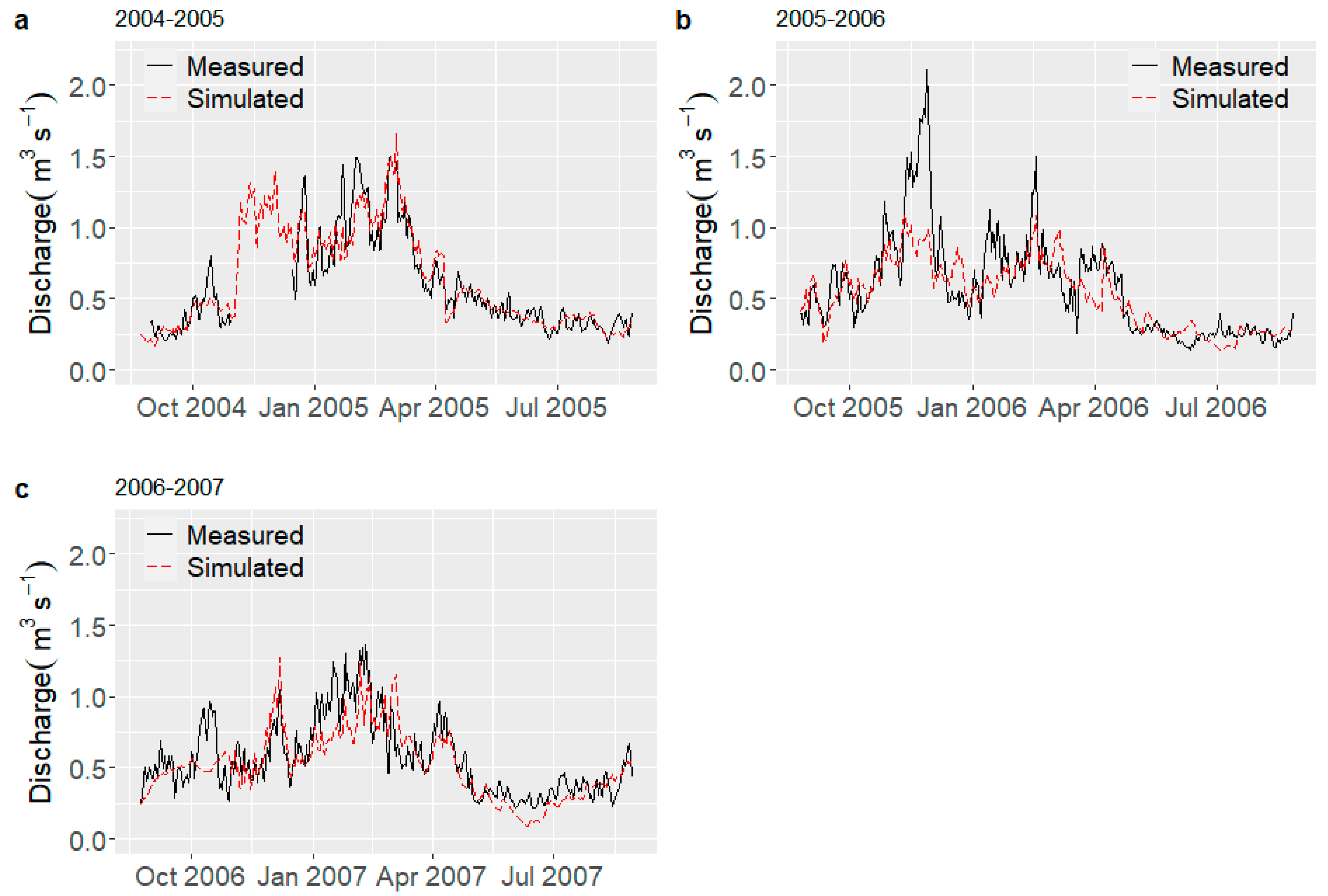
Figure 3 shows the performance of the calibrated model for the three hydrological years in terms of the Nash Sutcliffe coefficient (
E) and the
RMSE for the fitted discharge. Based on these values, the adjustment goodness is marked in the last column of
Table 3 using the general quality classification for
E of Cabrera (2009) [
42]. The lowest
E and maximum
RMSE are obtained in the year 2005–2006, but the adjustment quality is still considered as good.
The observed and simulated discharge hydrographs for the various years analyzed (2004–2007) are illustrated in
Figure 3. One may note from the different panels that the model cannot represent well the most prominent discharge peaks, especially, in the month December 2005–2006 and, to a lesser extent, some peaks of October and April of 2004–2005 and 2006–2007. For the hydrological years 2004–2005, 2006–2007, and the months of ASOND of the year 2007, the major discrepancy occurs in October. Significant bias in the estimation of some minima occurs mainly in the months of January and February 2005–2006, 2006–2007, and 2004–2005. These differences may be a consequence of disregarding the rapid fluctuations of albedo that could be produced by quick changes in precipitation [
43,
44]. However, the characteristic trends of the season are captured by the seasonal albedos, i.e., despite the use of seasonal albedos in the simulation, the performance of the model to simulate the discharge appears to be good enough. In fact, albedo parameterizations of the present DEBAM model [
45] require an hourly resolution of the input data, but not all climate variables for the CB are available with that resolution. Albedo simulations may be particularly important in the rainy season when the reflection of shortwave radiation varies more strongly over the days.
Nonetheless, the use of seasonal albedos for each surface appears to be warranted for calculating the typical average discharge in an acceptable way and, consequently, the amount of water produced by the glacier. Moreover, the simulation does not estimate subsurface energy transfer and subsurface flows, due to a lack of data in that regard. For instance, the subglacial flow of melting through channels could be enhanced in the core of the wet season, when there is more water in the snow [
46]. This uncertainty of the amount of subglacial flows could be at the origin of the observed underestimations of peak discharges in
Figure 3.
3.2. Stake and Pits Measurements, Mass Balance Profiles, Annual Mass Balance, and ELAs
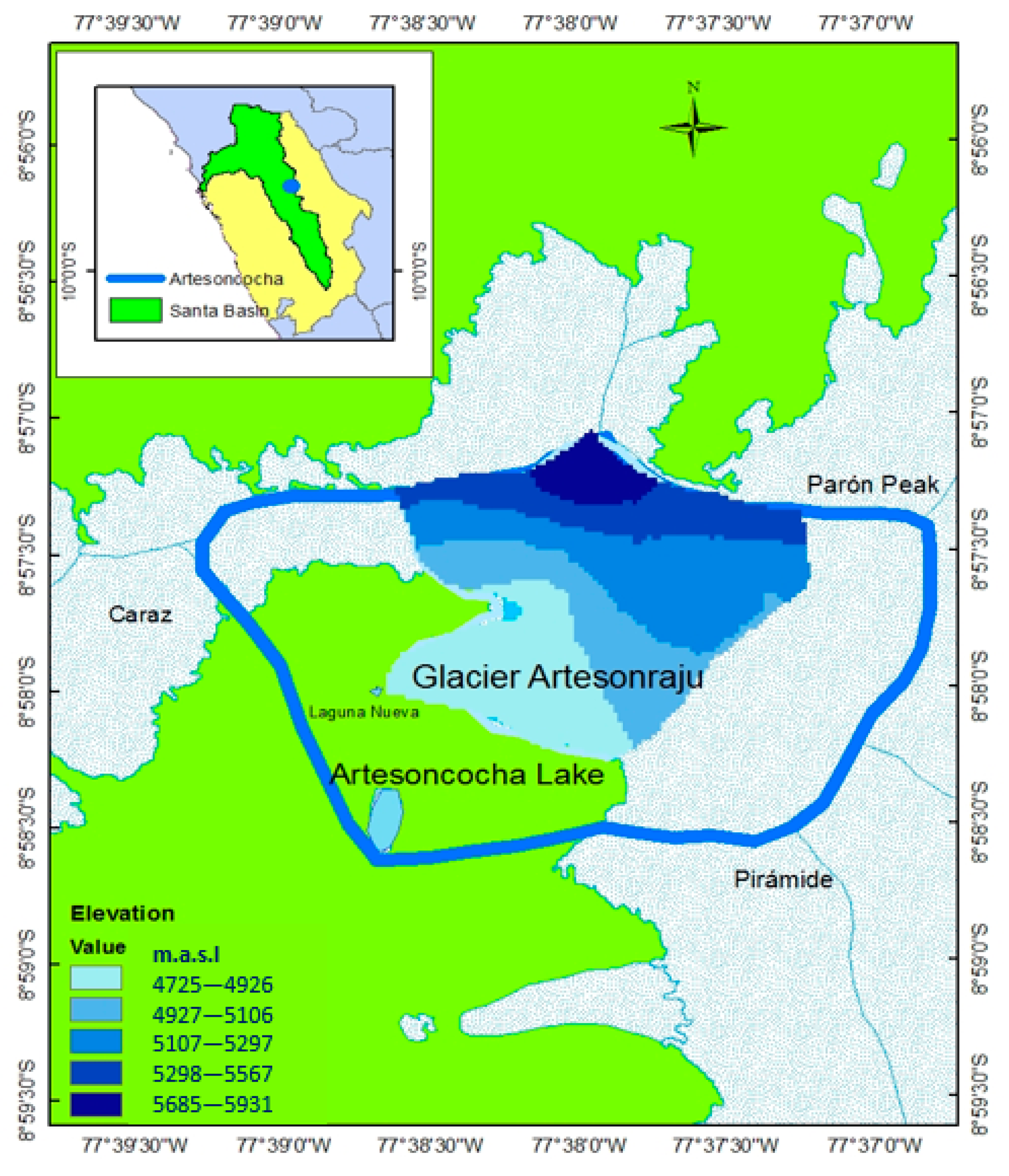
The mass balance is calculated only for the Artesonraju glacier, excluding some snow-covered areas of the Piramide, Paron, and Caraz peaks. These excluding areas also contribute to the discharge but do not feed specifically the Artesonraju glacier. The calculation area for the mass balance is 3.5 km
2, with a DTM of 30 m resolution. This area corresponds approximately to the one used by the UGRH in its calculations [
35]. The simulated annual mass balances are compared with the ones measured UGRH.
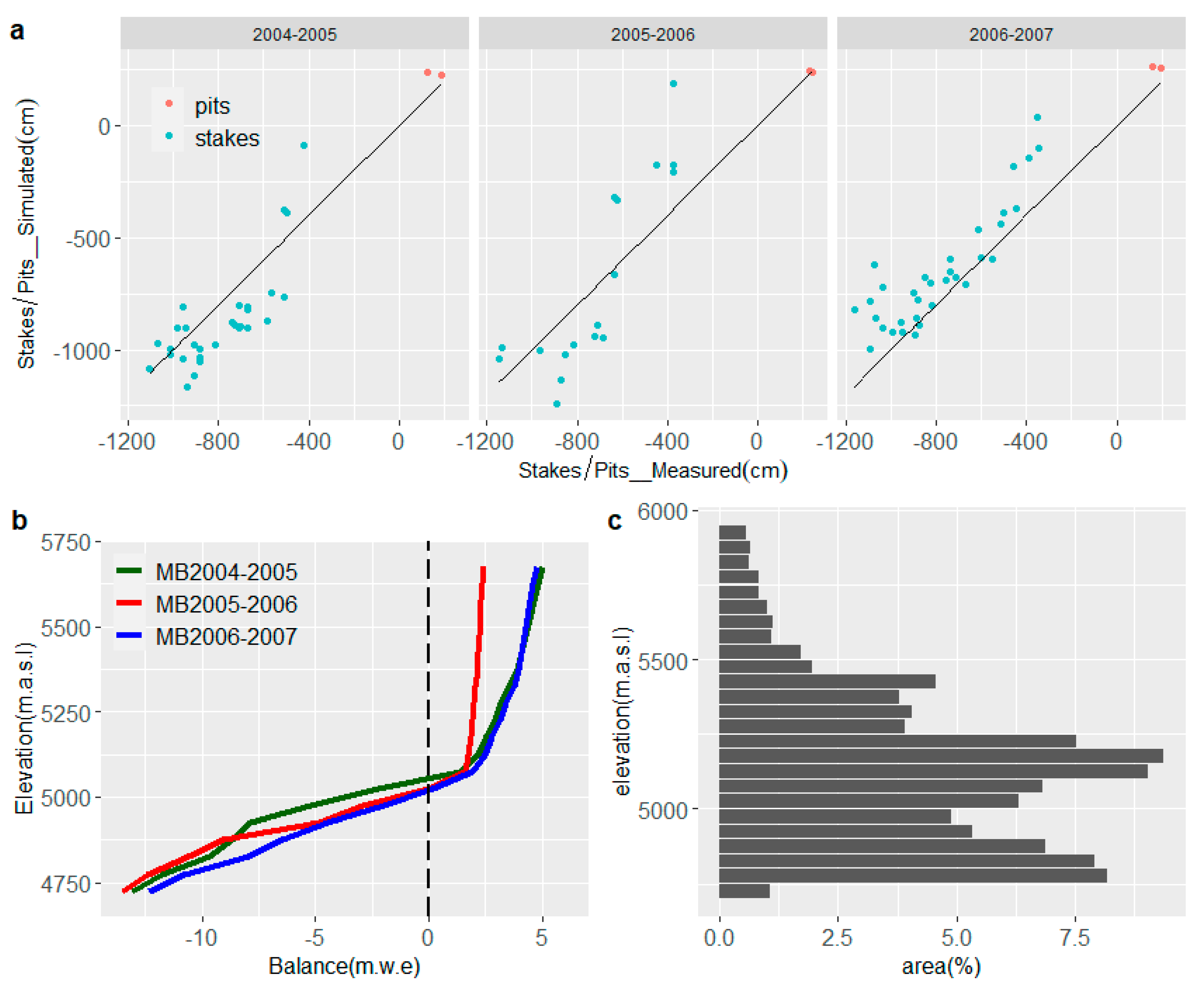
Figure 4a shows the cumulative mass at stakes/pits locations retrieved from the current simulation and
Figure 4b the mass balance profiles for each of the three hydrological years. The estimated
E and
RMSE for year 2004–2005 are 0.71 and 1.59 m, respectively; 0.58 and 2.36 m for 2005–2006; and 0.69 and 1.9 m for year 2006–2007. For all three years, the model performance in simulating the cumulated mass balance is good. The error is quite similar for the three years.
One may also notice from the different panels of
Figure 4 that for year 2004–2005, the energy balance model overestimates the amount of mass loss in the area of ablation. The contrary occurs in year 2006–2007, whereas in year 2005–2006, overestimations and underestimations of mass measurements occur alike. These outliers are most likely caused by the use of seasonal albedos in the model that cannot capture all changes that happen to the snowline position during the day. Moreover, the simulated mass in the accumulation area is very close to the measurements in the pits.
The ELA numbers listed in
Table 4 indicate a good agreement between the UGRH reported and simulated ELAs, with minimal differences between the two of only up to 35 m. This agreement is essential because the ELA separates the accumulation zone where snow and firn prevail from the ablation zone, majorly formed by ice. The 2004–2007 yearly displacement of the simulated ELA reveal the same pattern as the one of the yearly snow line identified by Rabatel et al. (2012) [
47] in Artesonraju (see
Table 4). Meanwhile, the UGRH- ELA estimations show opposite displacement for the years 2004–2005 and 2005–2006.
The simulated mass balance profiles (see
Figure 4b) unveil vertical mass balance gradients of ~4 m.w.e /100 m in the ablation area, but which decrease to ~0.5 m.w.e /100 m in the accumulation area. The estimations of the accumulation area ratio (AAR), defined as the ratio of the area of the accumulation zone to the glacier area, are also presented in
Table 4 and indicate variations ranging between 59% and 65% of the total glacier area. In fact, changes in the glacier zone areas have a significant impact on the estimations of the mass balances. However, glaciers with high slopes are less sensitive to AAR changes, as is the case for the Artesonraju glacier.
The simulated, mostly negative annual balances agree rather well with those estimated by UGRH (see
Table 4). Some minor differences occur in the year 2005–2006 when the simulated losses are lower than those estimated by UGRH. According to our model results, the largest yearly mass losses occur in year 2004–2005, whereas the UGRH-estimated losses are the largest in 2005–2006. However, these higher simulated losses for the first model year 2004–2005 are congruent to findings in the Zongo glacier, where the second-largest specific mass balances losses (after 1998–1997) were also measured in year 2004–2005 (−1.69 m.w.e.) [
48]. Moreover, the location of the snow lines [
47] shows steady increments of accumulated snow between 2004–2007. This trend indicates an increase in the accumulation area and, therefore, improvements in the glacier’s mass balance conditions towards the subsequent year 2007, all of which is in agreement with the current DEBAM simulations.
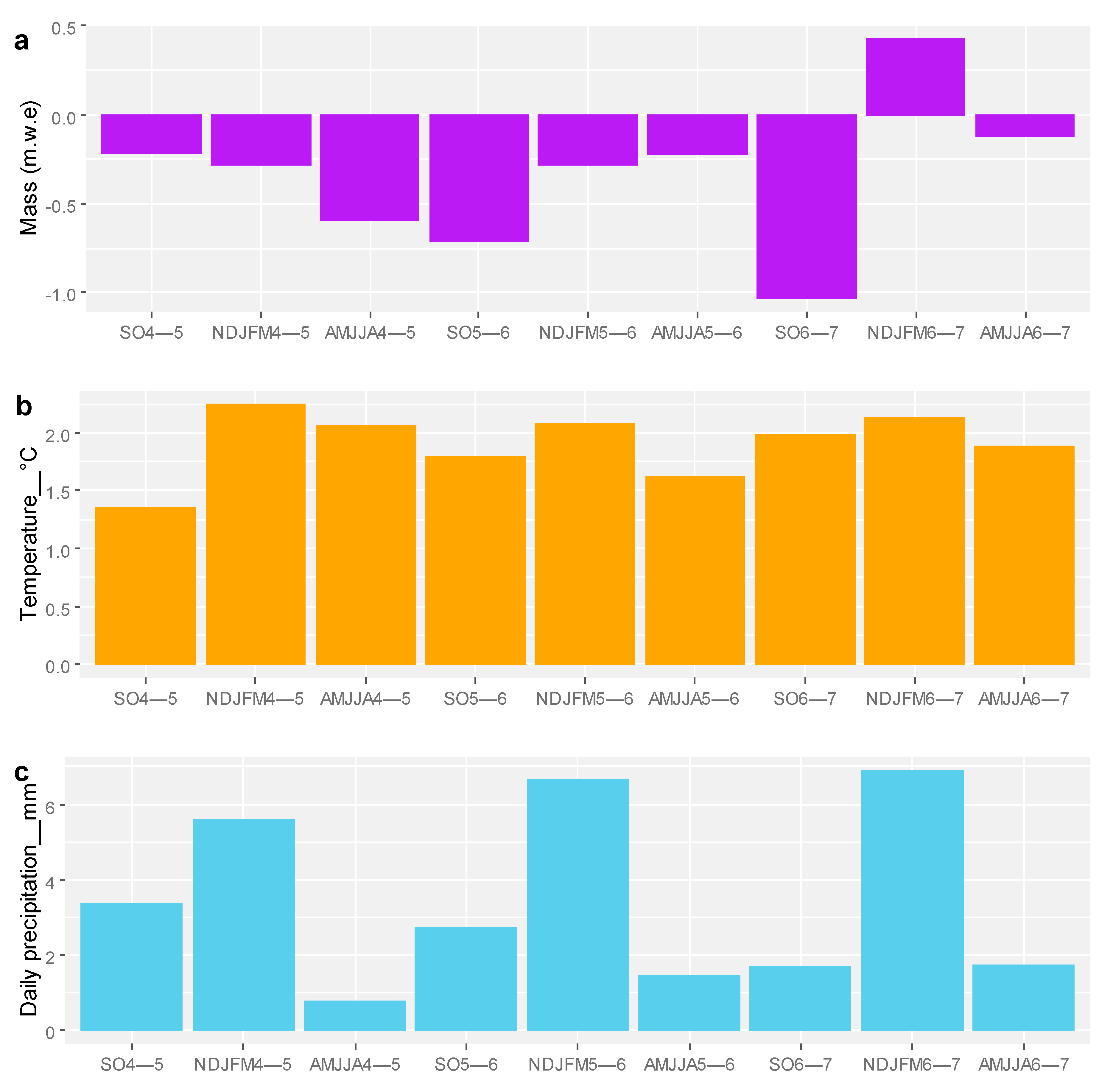
3.3. Seasonal Variations of Mass Balances and Association with Temperature and Precipitation
Figure 5 presents in a more detailed manner the seasonal variations of the simulated mean daily glacier mass balance, together with the mean daily temperatures and the mean daily precipitation. Generally, the steady mass losses obtained for all seasons in the year 2004–2005 and the beginning of the year 2005–2006 correlate clearly with seasonal increments of temperature and declines in precipitation for the periods NDJFM4-5, AMJJA4-5, and SO5-6, though this correlation is somewhat less stringent for the remaining seasonal periods between the years 2005 and 2007.
As the climate of the CB is strongly affected by ENSO tele-connection effects, the above findings can also be interpreted in terms of cyclic ENSO phenomena. Thus, a weak ENSO (El Niño) caused slight temperature increments and precipitation reductions in the CB in 2004–2005 [
49]. For example,
Figure 5 identifies the highest daily mass losses for season SO6-7, during which the precipitation was also significantly reduced. Indeed, one can observe that this season SO6-7 had the lowest precipitation from the beginning of the rainy seasons of all SO –periods in the 2004–2007 time span. Moreover, in this SO6-7 period, filled data of shortwave radiation incoming and longwave radiation was used. Ensuing small bias in this interpolated data produced increments in the calibrated threshold temperature
T0 (see
Section 3.4.2 later), which could lead to an overestimation of the mass balance loss in this SO6-7 period. Lagged cross-correlation analysis of ENSO- (El Niño SST) signals of Pacific Region 3.4 with climate time series in the CB by the authors [
34] show a lag of one to four months between ENSO anomalies and their effects on the glacier areas of CB. Therefore, the El Niño of 2004–2005 probably extended its teleconnection until SO5-6 in the glacier, with lower precipitation and slightly higher temperature in that period.
In contrast, during the year 2005–2006, a Niña event occurred during October to April in Niño 3.4 Region [
49], which can have a lagged effect in the glacier with a delay of up to 7 months. This Niña caused slight and steady increments of the precipitation that allowed the glacier to reduce losses in the first 9 months of year 2005–2006. Again, between August and January of the year 2006–2007, a weak Niño occurred in the Nino 3.4 region, which may have had a slight effect on the season AMJJA6-7. All these findings support the general idea that mass balances in the CB glaciers are significantly affected by El Niño/La Niña events [
3,
13,
22,
23,
50], wherefore, in particular, the here observed and simulated seasonal mass balance of the Artesonraju glacier may be explained in part by intermittent occurrences of such ENSO phenomena.
The above results indicate that in the simulated 2004–2008 time period, the glacier is far from reaching equilibrium. During most of the seasons in that time span, the glacier experienced losses of mass, though with alternating negative and positive trends, triggered by ENSO phenomena. As the changes in the Artesonraju glacier’s simulated mass balance also have indirect effects on the observed and simulated discharge at the outlet of its catchment (Artesoncocha lake), further analyses of the possible cross-correlation of the measured discharge with various climatic factors resulted in a correlation coefficient of r = 0.35 of the former with temperature at the climate station of Artesonraju glacier, of r = 0.43 at climate station Artesoncocha, and of r = 0.24 with Rh (relative humidity), of r = 0.26 with Lwinc, and of r = 0.28 with precipitation. Although these correlation coefficients may not appear too significant, they are basically consistent with the findings above regarding the effects of different seasonal climate variables (temperature and precipitation) on the glacier’s mass balance.
3.4. Model Calibration, Optimization and Sensitivity Analysis
The optimization of the DEBAM model was made by fine-tuning pairs of different input parameters (see
Table 2). Initial model simulations indicated that the assumed albedo value
of the different glacier surface types (snow, ice, firn), the threshold temperature rain/snow
T0, had a very strong impact on the model results for mass balance and discharge—and for the latter, also directly the storage constants
k for the three surface types of the routing reservoir model—as quantified by the ensuing
E and
RMSE-values (see
Table 3). For better manageability and illustrative purposes, these three most sensitive parameters of the model were mostly tested in pairwise combinations, and the corresponding results are presented and discussed in the subsequent paragraphs.
3.4.1. Albedo
Different combinations of albedos for each of the glacial surfaces were tested, but by respecting the physical ranges of their possible values. The model sensitivity to the seasonal albedo selection was also investigated under different threshold temperature T0 conditions.
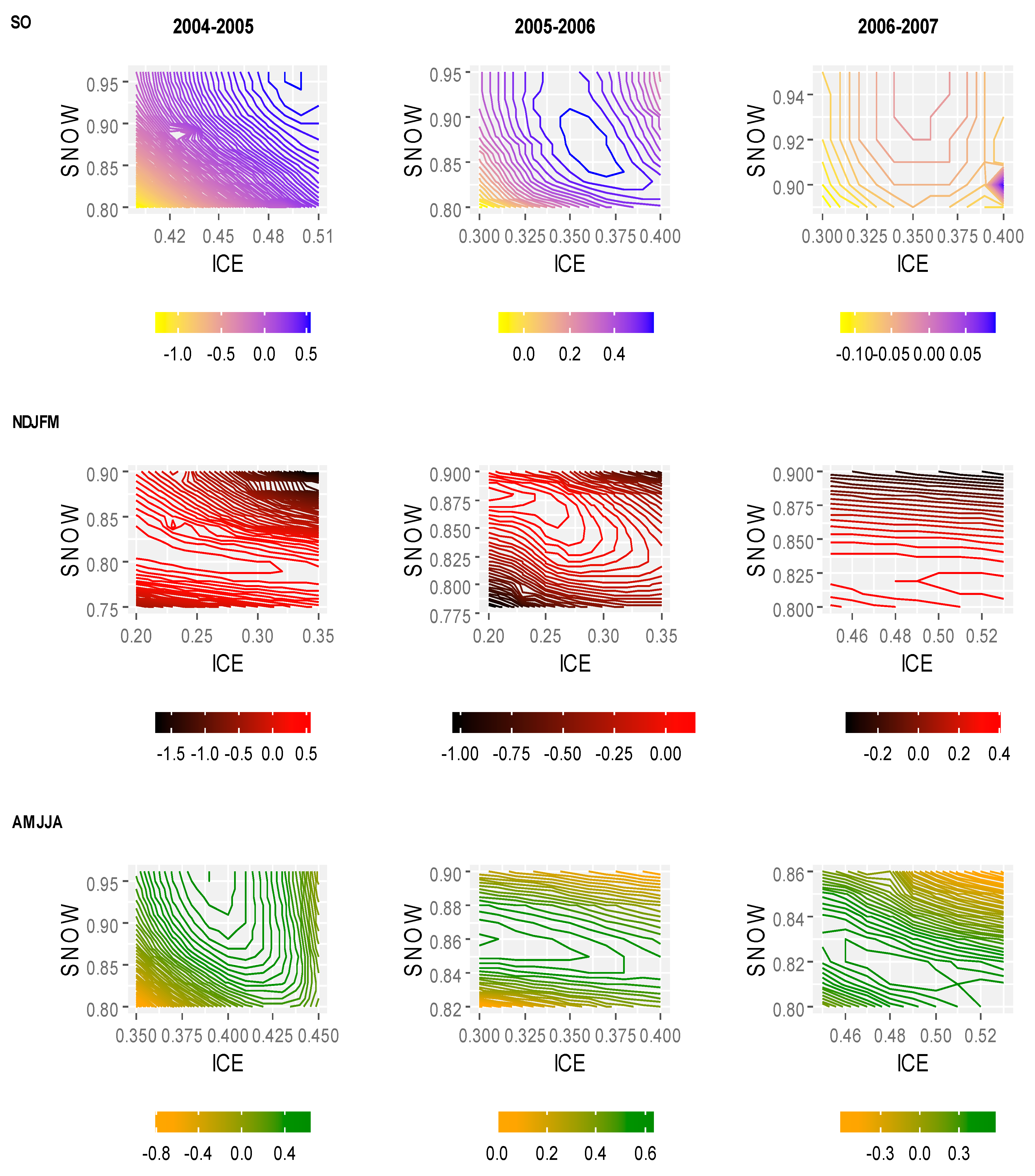
Figure 6 shows the response surfaces of the Nash Sutcliffe parameter
E of the simulated discharge for different combinations of snow and ice albedos for each season of the three-year simulation period. Generally, one can notice for all three years similar tendencies of the
E response surfaces for the same season.
More specifically, for the SO seasonal period, high calibrated values of the snow albedo are observed, varying from 0.90–0.95, whereas that of ice ranges between 0.35–0.5. This seasonal high albedo can be explained by the beginning of the wet season in which fresh snow is typical and clean ice prevails in the ablation zone.
For the subsequent wet season period NDJFM, the snow albedo decreased to a range of 0.80–0.88. The same holds for the ice albedo, which declined to 0.25–0.3 for years 2004–2006, but increased again to 0.45–0.5 for 2006–2007. In this wet season, more significant fluctuations of precipitation and a slightly higher temperature usually occur, so that the glacier melting is higher. The ensuing meltwater reduces the snow albedo directly and indirectly increases the grain size of the ice/snow surface which, in turn, reduces albedo [
43]. The above albedo fluctuations are consistent with typical values from fresh snow and wet snow [
37].
Lastly, for the AMJJA dry season period, the snow albedo ranges between 0.82 and 0.95. During that timespan of low precipitation, the water content is reduced, maintaining the snow accumulated in the previous season. Therefore, the snow albedo tends to increase compared with the previous season, which is also concordant with what was observed by Juen [
15]. In fact, in the present case, two of the simulated seasons between 2005 and 2007 are characterized by (lower) albedos of old dry snow.
3.4.2. Threshold Temperature Rain/Snow T0
The threshold temperature rain/snow (
T0) determines the surface or size of the areas of snow, ice, firn, and debris which, in turn, by their different physical features, influence the overall energy budget of the glacier. Generally,
T0 is variable and depends on geographical and seasonal atmospheric conditions. The latter influence the state of precipitation through different mechanisms. For example, the thickness of the air layer that falling water droplets (leading to precipitation) must go through, the soil heat, the cooling influence on humidity, and the salt content of the particles affecting freezing point are some factors that influence the type of precipitation eventually reaching the soil [
51,
52,
53]. A study with over 1000 climate stations in the United States of America showed that rain never occurs beneath a temperature of 0.8 °C and that snow is never observed, when the temperature exceeds 6.18 °C [
54]. Observational data in the northern hemisphere indicate that the warmest threshold temperatures occur in certain mountain regions above 4000 m.a.s.l., e.g., Rocky Mountain 3.8 °C and Tibetan Plateau 4.5 °C [
55]. Another study, specifically in the Cordillera Blanca of interest here, estimated a rain/snow threshold temperature range of 1.1–2.5 °C in the Shallap glacier [
14].
Based on these studies, it is of no surprise that
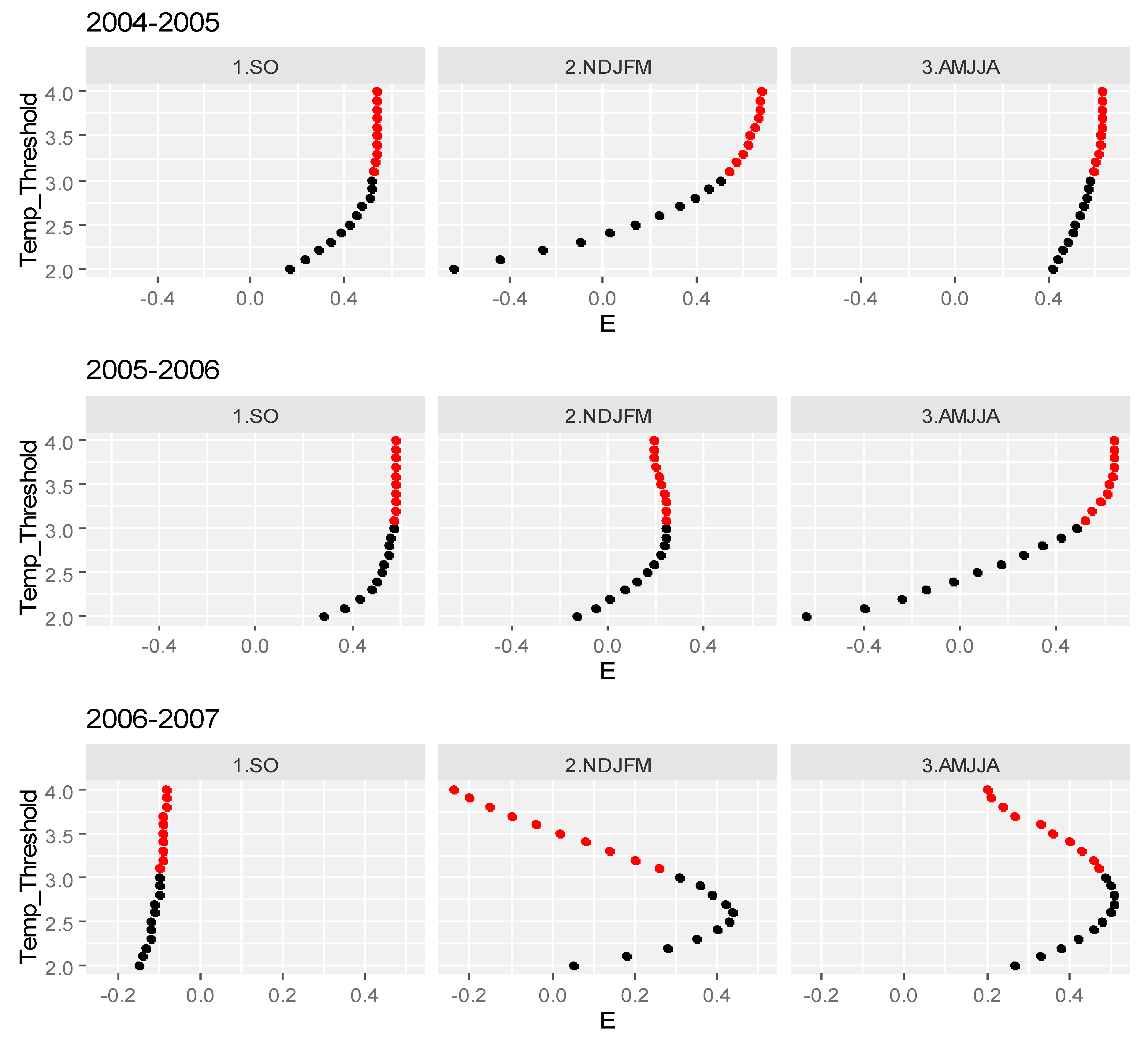
T0 turns out also to be a very sensitive parameter in the present model simulations, as illustrated by
Figure 7, which shows the seasonal
T0 sensitivity for the three hydrological years in terms of its effect on
E.
Figure 7 reveals that the best seasonal rain/snow threshold temperature
T0 ranges between 2.6 °C and 3.8 °C, which are higher values than those found above in glacier Shallap [
14]. These disagreements may be due to uncertainties in the spatial variation of other climate variables, such as precipitation, wind, relative humidity, vapor pressure, and daily snowfall variability. Moreover, any deviation of the assumed initial conditions from the real limits of the different surface types can be compensated by increasing the threshold temperatures.
Eventually, ENSO anomalies can also produce changes in
T0. For the CB study region, an ongoing El Niño event usually leads to strong dryness—as is the case, for instance, for the one occurring during NDJFM and AMJJA in year 2004–2005, when higher seasonal daily mean temperatures and lower daily precipitation occurred (
Figure 5). In fact, snowfall events at a lower relative humidity are more likely to fall as snow at higher
T0, i.e., 4.5 °C (40–50%), 3.7 °C (50–60%), 2.8 °C (60–70%), 2.2 °C (70–80%), 1.4 °C (80–90%), 0.7 °C (90–100%) [
55]. As for the glacier Artesonraju, the seasonality relative humidity shows reductions, especially in the dry season, to 62–75%, compared to 74–80% in the wet season, all of which is in tendency with the present results (
Figure 7). In general, as the relative humidity in the Artesonraju glacier turns out to be slightly lower than that in the southern glaciers of the CB [
34], the higher
T0 modeled here are understandable. Notwithstanding,
T0 could be overestimated in the model calibration, compensating for any uncertainty or inaccuracy in the input data, as mentioned above, i.e., bias in the delimitation of the different surface areas, but also uncertain precipitation losses and gradients.
3.4.3. Discharge Storage Constants
The optimal discharge storage constants
k of the reservoir routing model (Equations (9) and (10)) obtained as part of the sensitivity study for the three glacier surfaces and the different seasons are listed in
Table 5. Similarly to the two previously discussed sensitivity parameters, the spread of the storage constants across the three years simulated is relatively low for the same season. However, differences arise for the individual seasons. Thus, for the first season, SO, values of
kfirn of 700–800 h, for the second (rainy) period, NDJFM, of 500–800 h, and for the third (dry) season, AMJJA, of 1100 h are obtained. The storage constants of firn are consistent with the cycle of firn formation in the hydrological year, i.e., maximum values at its end in the dry season (AMJJA), when a larger residence time prevails, owing to more snow accumulation (and conversion to firn) from the previous season. The lower
kfirn—values obtained for season NDJFM can be explained by the fact that more melting water penetrates into the firn’s interstices. In the first (2004) SO season, on the other hand, the melting is still low, and the firn formed in the preceding season still prevails, which leads to a slightly larger
kfirn-value.
For ksnow, the seasonal ranges are 390 h, 390–900 h, and 150–200 h for seasons SO, NDJFM and AMJJA, respectively; i.e., the ksnow-values for the two rainy periods SO and NDJFM are much larger than that of the dry season AMJJA. This is due to the fact that there is more snow during the two rainy seasons and which is maintained for a longer time period. Indeed, for tropical glaciers, the total snow accumulation of a year occurs in these two rainy seasons.
Finally, for kice, values ranging between 30 and 50 h for NDJFM (wet season) and of 250–300 h for AMJJA (dry season) are encountered. This is congruent with large melting and ensuing discharge in the wet season, resulting, consequently, in a lower residence time for ice, but lower melting and discharge in the dry season, i.e., a higher residence. However, for the season SO of 2006–2007, an extremely high value of kice = 500 h is found that may not be realistic and is most likely due to some gaps in the input data during that period which, though filled in, as discussed earlier, may lead to some modelling errors.
Table 5 shows further that the highest storage constants are obtained in the dry season (AMJJA), mainly for firn and ice surfaces. This is logical, as during that season, the glacier receives less energy input (southern winter) and, thus, less melting takes place, ergo, less discharge at the glacier’s outlet. Interestingly, the situation is somewhat opposite for
know, where, for the dry season, the
k values are the lowest. Indeed, as the solid precipitation is also reduced in that dry season, the sporadic snowfalls can melt faster, leading to a shorter snow storage time.
In conclusion of this section, it can be stated with some confidence that the optimally calibrated discharge storage constants represent the seasonality of accumulation and ablation of snow, ice, and firn, typical of the outer tropical glaciers, satisfactorily.
3.5. Contribution of Seasonal Energy Fluxes on the Melting Energy Balance
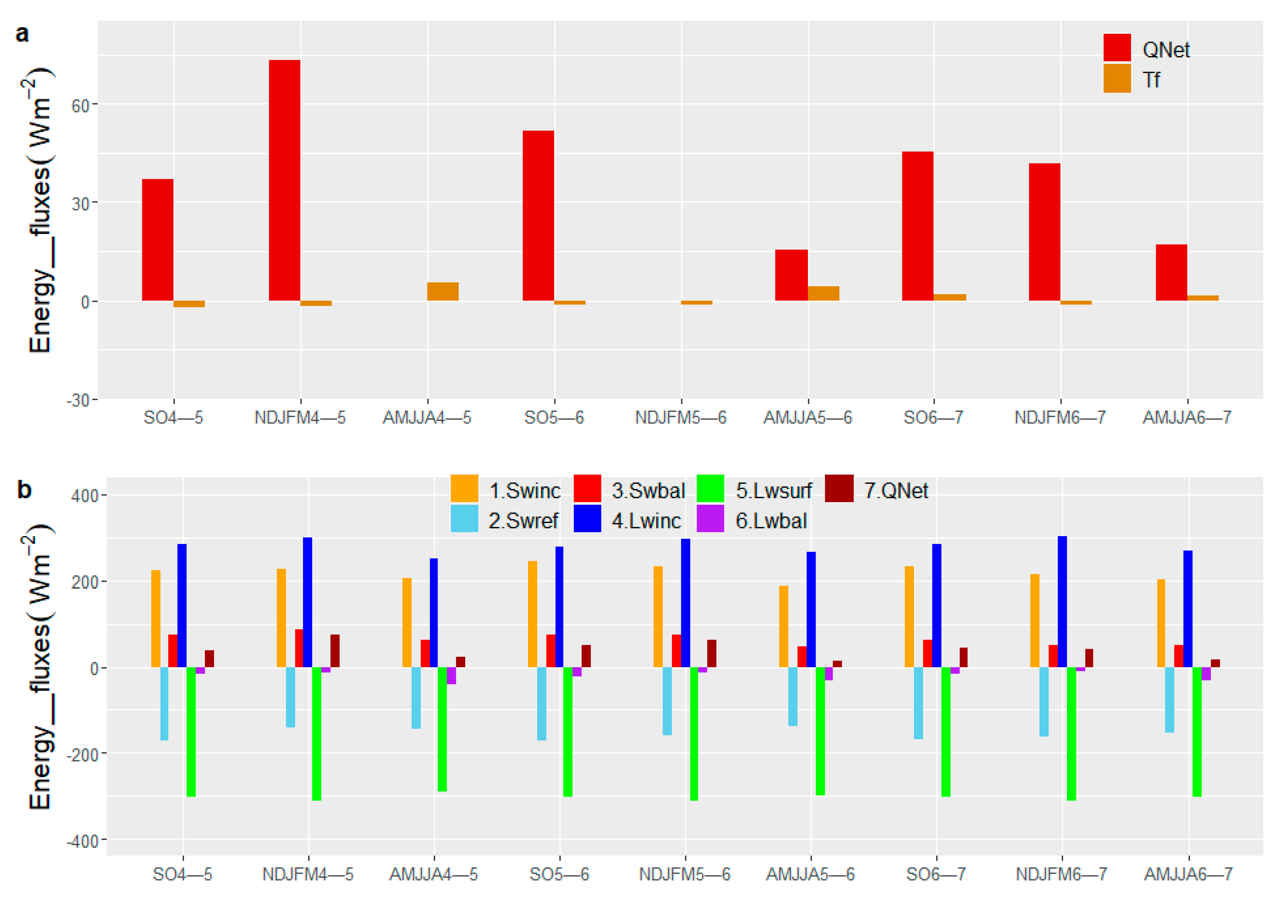
The mean seasonal contributions of the different radiation energy flux terms to the overall energy balance of the glacier (Equation (1) and following) for the whole 2004–2007 simulation period are presented in
Figure 8a, which indicates that the net radiation (
QNet), which eventually drives the total mass losses on the glacier’s surface, ranges between 15 and 73 Wm
−2, depending on the season. In particular,
QNet decreases in all dry seasons of the simulated years. This seasonal variation of
QNet is consistent with the typical seasonal cycle of ablation of the outer tropic glaciers.
Figure 8b shows in more detail that lower shortwave balance (
Swbal) and longwave balance (
Lwbal) in the dry and cold seasons leads to a large decline of
QNet, which, obviously, reduces glacial melting.
The net shortwave radiation balance (
Swbal) has the most significant weight within the net radiation term (Equation (2)). Although there is more precipitation in the wet seasons (
Figure 5), the calibrated albedos of the snow surfaces have similar seasonal values in the core wet season and the dry season (see
Section 3.4.1). In the wet seasons, not only does more snow precipitation fall, but the latter also has a larger water content. This occurs during a time period of maximum net radiation and slightly increased temperatures (
Figure 5). All this could reduce the snow albedo values for the wet season a bit. Nevertheless, the mean shortwave radiation reflected (
Swref) (Equation (3)) of the whole glacier is comparatively larger in the two wet seasons than in the dry season. This can be explained by the fact that, during the dry season, the overall snow surfaces of the glacier shrink, reducing its average total reflection (lower
Swref).
Swbal is generally higher in the rainy (51–86 Wm−2) than in the dry (43–63 Wm−2) season. Moreover, Swinc decreases slightly after the rainy seasons during the simulation years 2004–2007. This reduction in the subsequent dry seasons is to be expected, as with then lower precipitation and less cloudiness, diffuse incoming radiation diminishes.
As for the net longwave radiation (
Lwbal), one can notice from
Figure 8b that it is also reduced for the dry seasons. For the latter, the diagrams show, furthermore, that
Lwbal makes up about 63%, 73%, and 66% of the
Swbal energy received in years 2004–2005, 2005–2006, and 2006–2007, respectively. This overall dry-season reduction of
Lwinc, necessarily, causes an even more significant drop of
Lwbal during that time period, when there are more clear sky days.
It should be noted, finally, that these findings regarding the seasonal variations of longwave radiation balance in the Artesonraju agree well with those obtained for the Zongo glacier [
19]. Further comparisons with other studies will be made in the subsequent section.
The seasonal mean of
Tf (comprised of the sensitive heat
QHS as well as the latent heat
QHL, see Equations (4) and (5)) increases a little in the dry seasons of 2004–2005 and 2005–2006, compared to the wet seasons (
Figure 8a). These seasonal increases (mainly of
QHS) may be the result of temperature rises in the named seasons due to the then-occurring El Niño phenomenon.
3.6. Comparison of Simulated Energy Balances with Those of Other Studies in Tropical Glaciers
Averaging the seasonal flux terms of
Figure 8b over the year, the corresponding values, as listed in
Table 6, are obtained. Our estimations of the energy fluxes
Swinc,
Lwinc and
Lwsurf are quite similar to other studies carried out in the Andean tropical glaciers. Energy fluxes in the glaciers of Zongo, Antisana, Shallap, and Artesoranju for different years [
3,
10,
11,
12,
16,
17,
21,
22,
56] show that the annual averages of
Swinc range between 206 and 239 Wm
−2,
Lwinc between 258 and 310 Wm
−2, and
Lwsurf between −277 and −311 Wm
−2. Our annual averages for these variables are within the mentioned ranges.
On the other hand, the mean annual reflected shortwave radiation (
Swref) range of 151–162 Wm
−2 tends to be a little above the average range estimated in the mentioned studies of tropical glaciers (−86–137 Wm
−2). Nonetheless, this discrepancy may be partly understood by considering that (a)
Table 6 shows annual averages of shortwave reflected in the whole area which, keeping in mind that the AAR is between 59 to 65% (
Table 4), the albedo in the accumulation area, which is predominantly high, raises the average, whereas some of the other studies presented site values; (b) different local climatic conditions could occur in the tropical glaciers, for instance, in the CB the influence of charged air masses that ascend from the eastwards located Amazon basin may also be felt in the Artesonraju glacier (indeed, there is a low correlation of the precipitation within some subbasins in the CB); (c) the use of seasonal albedos may influence the results obtained for
Swref, since daily fluctuations are not captured; (d) the uncertainty in the assumed precipitation gradients is high, as there are no gauge stations in high elevations of the glacier. Notwithstanding, the simulated
Swref values at the climate station are similar to the measurements there. The turbulent fluxes (
Tf) found here (
Table 6) are between the ranges found for other tropical glaciers, in which
QHS is between −2 and 21 Wm
−2 and
QHL between −27 and −4 Wm
−2. Generally, the turbulent fluxes
Tf are comparatively less than the net radiation
QNet, which is due to the fact that, over the whole year (but not for separate seasons), the mean daily sensible (
QHS) and latent heat (
QHL) fluxes counterbalance themselves pretty much, here, with their sum (=turbulent fluxes,
Tf) hovering between +1 and 0 Wm
−2.
3.7. Vertical Profiles of Seasonal Energy Balance Flux Terms across the Glacier’s Elevation
In the present sub-section, vertical variations (profiles) of the various simulated seasonal energy balance flux terms in the across the glacier elevation range are presented. To that avail, maps of the simulated mean seasonal distributed energy fluxes, with a horizontal resolution of 30 m × 30 m, are divided into elevation bands, each of which covering a range of 50–60 m of elevation, resulting in a total of 24 bands across the whole glacier altitude range. A mean energy flux is then calculated from the aggregated grid point values in one elevation band. Vertical profiles of the different seasonal energy flux terms obtained in this manner are shown in
Figure 9,
Figure 10 and
Figure 11.
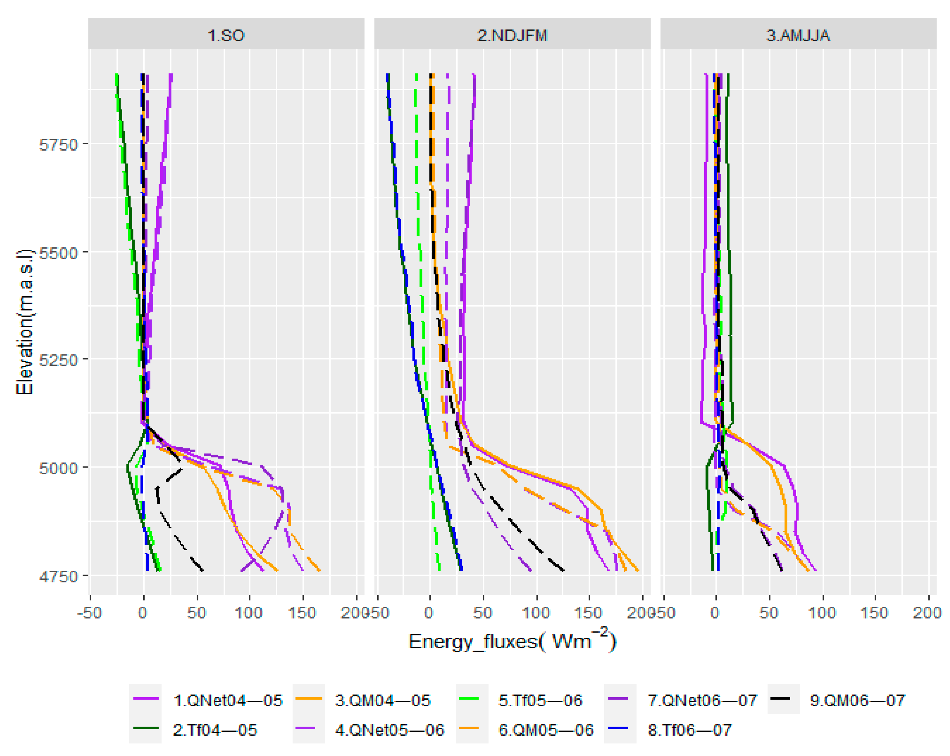
The vertical profiles of
QNet (Equation (2))
Tf (Equations (4) and (5)) and the ultimate energy remaining for melting
QM (Equation (1)) are illustrated for each season of the 2004–2007 simulation period in
Figure 9. The three panels depict the results for the three seasons of the hydrological year, but for each year individually, allowing to better follow the seasonal time evolution of the energy flux terms across the analysis period.
One can notice from
Figure 9 that
QNet is much more prominent in magnitude and more variable (ranging between −1 and 177 Wm
−2) in the lower-lying ablation zone than in the higher-lying accumulation zone (ranging between −15 and 43 Wm
−2). This pattern is congruent with the typical minimization of mass losses in the accumulation zone and maximum mass losses in the ablation zone. Moreover, low
QNet radiation occurs in the accumulation zone occasionally at the beginning of the rainy season (SO) and predominantly in the dry season (AMJJA).
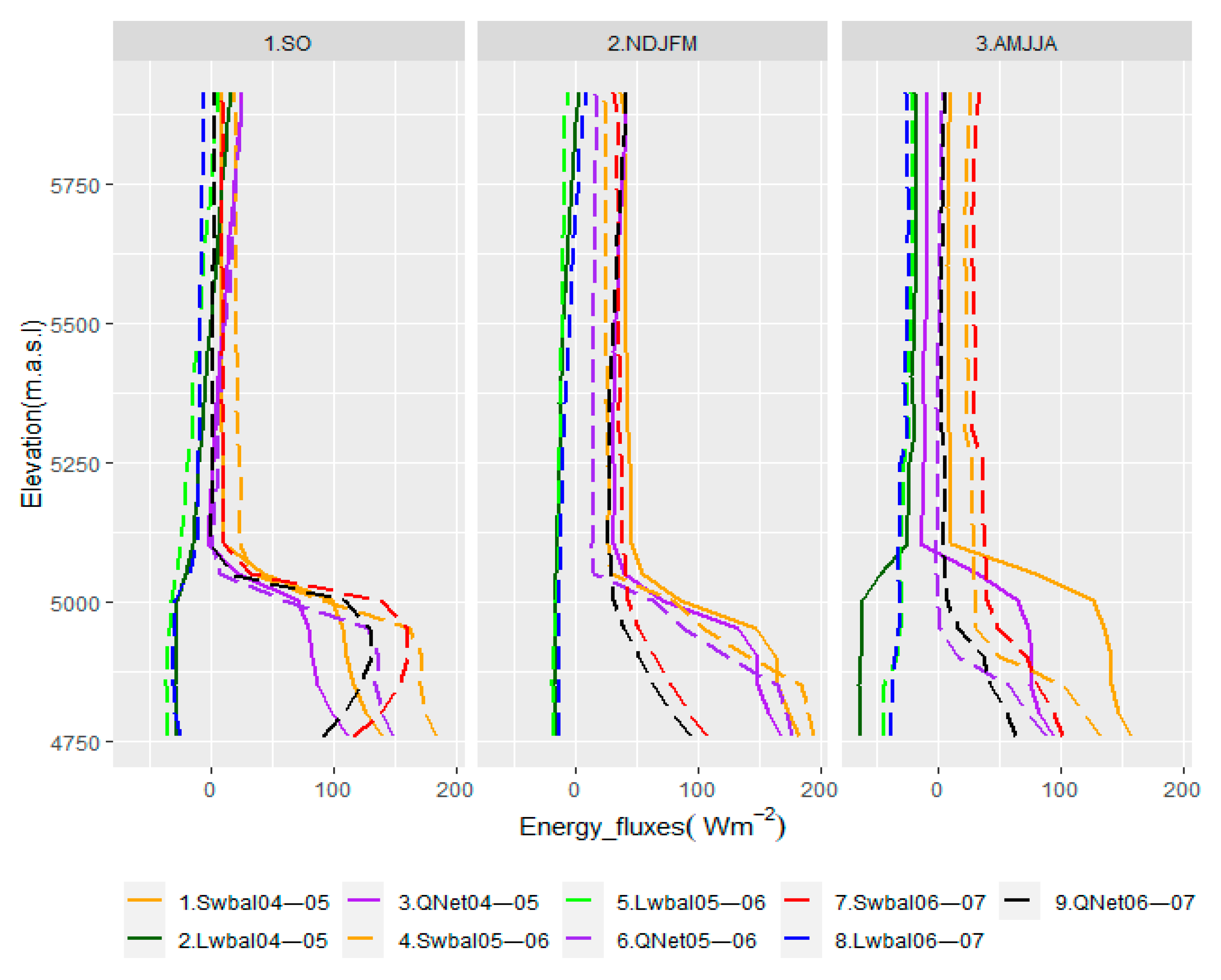
The peculiar vertical and seasonal variations of
QNet across the glacier’s elevation are a direct consequence of the underlying definition of
QNet as the sum of the shortwave (
Swbal) and longwave (
Lwbal) radiation balance (Equation (2)). The vertical profiles of these two radiation fluxes are depicted in
Figure 10. From this figure one can notice that high values of
Swbal (between 30 and 194 Wm
−2) occur in the ablation zone. In contrast, in the accumulation zone, these values are low (between 7 and 79 Wm
−2) due to the increased albedo here (Equation (3)), which is characteristic of this zone (snow). On the other hand,
Lwbal values differ less between accumulation (between −46 and 17 Wm
−2) and ablation (between −66 and −12 Wm
−2) areas, and this holds for all season. As these
Lwbal values are predominantly negative across the whole glacier, particularly in the ablation area, where surface temperatures of 0 °C prevail, it becomes clear that the longwave radiation balance is not responsible for any glacier melting. This means, last but not least, that
QNet in the ablation area is controlled by the shortwave radiation balance (
Swbal).
The magnitude of the
Tf flux terms in the two zones is less variable than that of the
QNet. However, these fluxes tend to be higher (ranging between −16 and 30 Wm
−2) in the ablation zone than in the accumulation zone (ranging between −40 and 15 Wm
−2). In the latter,
Tf is predominantly negative for both rainy seasons (SO, NDJFM), but also shows more significant variations (ranging between −40 and 15 Wm
−2) and which are reduced again in the dry season (AMJJA) (between −2 and 15 Wm
−2). This reduction suggests the strong influence of wind on
Tf, rather than relative humidity and temperature. Wind increases in the wet season, whereas relative humidity and temperature decrease in the dry season [
34]. Furthermore, as
Tf is not high in the ablation zone (between −16 and 30 Wm
−2), compared to the
QNet radiation term (between −1 and 177 Wm
−2), the former flux term does not drive the melting in this zone.
However, the situation is different for the accumulation zone, where the
Tf profiles suggest that they may act as a significant sink of energy, especially in the beginning and the core of the wet season (see panels SO and NDJFM of
Figure 9 discussed above); i.e.,
Tf offsets the effects of
QNet in that zone. This energy sink represents the glacier mechanism to minimize the melting in the accumulation zone in the wet season (SO, NDJFM), in spite of higher radiative energy input during that period. Indeed, in the dry season (AMJJA),
QNet is reduced due to lower back-emission of longwave atmospheric radiation (
Lwinc) and slightly less incoming short wave solar radiation (
Swinc).
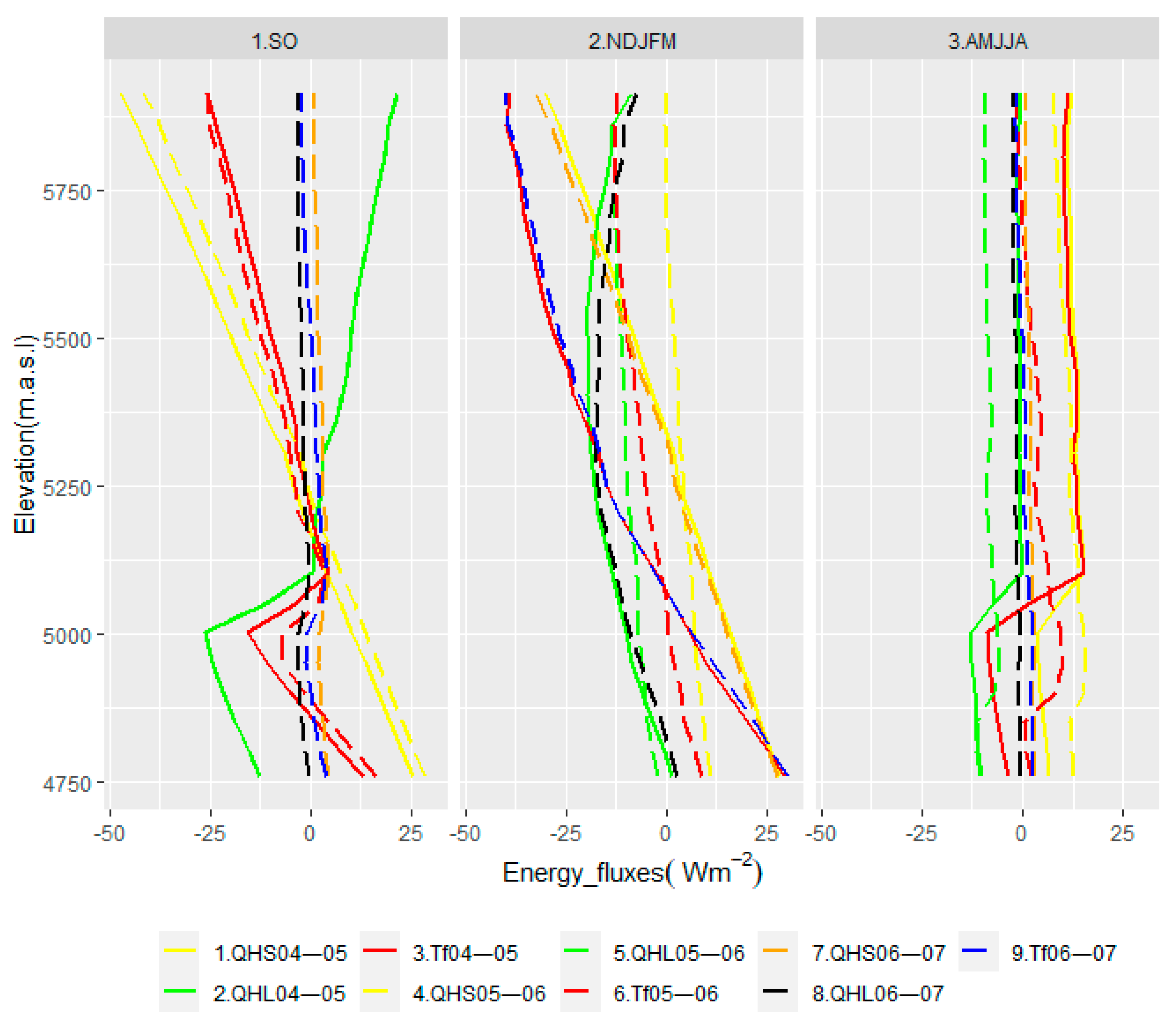
A more detailed picture of how the turbulent flux
Tf is divided across the glacier’s elevation into its two components,
QHS (sensible heat) and
QHL (latent heat), is presented in
Figure 11 The sensible heat
QHS varies between 2 and 29 Wm
−2 in the ablation zone and between −47 and 15 Wm
−2 in the accumulation zone; i.e., it is mainly negative there, particularly during the wet season. On the other hand,
QHL is positive in SO, resulting in a loss of energy that enables deposition processes, but negative in NDJFM, generating energy for sublimation which requires eight times more energy than melting. Due to this, melting in the accumulation zone is prevented, although higher
QNet is available in these two wet seasons. Additionally, as already mentioned for
Figure 9,
Tf is lower in the dry season which, by virtue of
Figure 11, can now be explained by the fact that the two heat flux terms
QHS and
QHL counteract each other more or less over the elevation range of the glacier. Nevertheless, slightly higher values of
Tf are obtained in the dry season of the two El Nino years 2004–2005 and 2005–2006, due to small increments of
QHS.
In conclusion, the vertical profiles of the various energy balance equations terms presented in this sub-section allow to clearly distinguish the ablation (ice-covered) and accumulation (snow-covered) zones across the elevation of the glacier and their development over the various seasons of the analyzed 2004–2007 time period.
3.8. DEBAM Glacier Simulation Uncertainties and Their Possible Sources
The current DEBAM glacier simulations, in conjunction with the limited quantity and quality of the input and calibration data, are naturally fraught with some uncertainty and/or errors. One particular source of the latter may be the scarcity of mass-balance- and radiation measurements in the accumulation zone of the glacier. In the high mountains of the Cordillera Blanca, these glacier zones are usually steep and abrupt, making access for measurements difficult, let alone dangerous [
33]. As the net and the instrumentation of the measurements are also costly, the latter generally cover just some parts of the glaciers [
3]. Therefore, initial conditions for use in the numerical model, especially those describing accumulations, are still difficult to estimate over the whole area.
Another source of uncertainty is the spatial variation of the various climatic variables, such as precipitation, wind speed, and relative humidity. Precipitation was assumed with losses ranging between 20 and 30%. The wind speed in the DEBAM is assumed as constant across the whole glacier modeling area, which has direct consequences on the proper estimation of the turbulent fluxes (latent and sensible heat), so that these are, necessarily, fraught with certain inaccuracies. The latter will then propagate into the estimation of the net energy flux available for melting. Thus, exploring different parameterizations to account for the spatial wind variability may be an essential task for a better understanding of the role of sublimation, condensation, deposition, melting, and other variables, all of which depend strongly on the wind speed. Moreover, the direct interference of strong wind blowing leads to a reduction of the net snow accumulation at high altitudes, although it may produce accumulation in topographic depressions (so-called snowdrift) [
3], both of which are out of the scope of the present model simulations.
The sporadic gaps in the measured energy flux time series filled with various statistical interpolation methods [
34] are also sources of uncertainty. The possible errors generated in this way could affect the performance of the DEBAM model, as is reflected by the (relatively low) Nash Sutcliffe coefficients of the present simulations for the partly filled-in data of season SO of year 2006–2007.
Unknown daily variations of the albedo are another source of uncertainty. Indeed, variations of albedo are expected particularly in the wet season, due to the fact that strongly fluctuating precipitation amounts and moisture contents affect the permanence of the snow cover on the glacier’s surface. As a matter of fact, snow albedo falls exponentially after a few snowfall days [
43,
57]. However, such albedo changes are not considered in the current model.
The unknown amounts of energy transfers in the subsurface and the subglacial flows (see Equation (1)) are another source of uncertainty in the understanding of Artesonraju glacier dynamics and could contribute to an underestimation of discharge, especially in the wet season, when more water from melted snow flows downhill towards the outlet of Artesoncocha lake.
Finally, rock avalanches that produce significant changes of debris mass in high, abrupt mountains may affect the thermal environment on or near the glacier and so influence the dynamics of the latter. Such mass movements caused by massive slope failures (favored by rising temperatures, and so exacerbated by climate change) have been observed in high mountain glaciated areas of the alpine region [
58].
4. Conclusions
By means of a novel distributed energy balance model (DEBAM), the present glacier modelling study sought to deepen the understanding of the various physical processes with their leading parameters that govern mass balance in tropical glaciers—here, the Artesonraju glacier in the CB, Peru. Thus, the results of the present modeling exercise contribute to the yet existing and occasionally contradictory conclusions of many other previous studies in this field, regarding the dominant drivers of the seasonal dynamics of tropical glaciers, in general.
Based on the scarcely available empirical input data, a time period of only three years (2004–2007) was modelled. In spite of this rather short calibration period, good-to-satisfactory results are obtained, with the Nash Sutcliffe coefficient
E ranging between 0.60 and 0.87 for measured discharge at the Artesoncocha lake outlet (after fine-tuning the storage constants in the reservoir routing model in a seasonal manner) and of 0.58–0.71 for glacier stakes’ mass balance measurements. Moreover, annual mass balance estimations were compared with previous official calculations by UGRH [
35]. The simulated annual mass balances show mass losses between −1.42 and −0.87 m.w.e., which turns out to be concordant with the official estimations. The annual and seasonal balances strongly depend on climatic variations associated with El Niño and La Niña phenomena, which occurred during the time period simulated.
A more detailed analysis of the various components of the energy balance equations indicates that the net radiation (sum of short- and longwave radiation balances) governs the energy balance and the melting processes, confirming results of some current studies [
3,
10,
11,
14,
18,
19,
22]. More specifically, it is the reflected shortwave radiation which is the dominant component here. As the latter is governed by the albedo of the different glacier type surfaces (snow, ice, firn), further sensitivity studies with regard to that parameter were carried out. Although the daily short-term variations of albedo could not be simulated, the use of seasonal albedos for three different seasons (less rainy, rainy, dry) allowed to satisfactorily perform the modelling tasks. As a conclusion here, the seasonal albedos appear to reasonably account for the temporary characteristics of the surface conditions over the season under question.
On the other hand, longwave radiation still plays a role in determining seasonal glacier conditions, for instance, by reducing the radiation at the surface in the dry season when there are more clear sky days. This result is confirms statements of Sicart [
19].
Vertical profiles of various seasonal energy balance flux terms across the glacier’s elevation reveal particularly interesting details on the factors controlling the temporal dynamics in the glacier’s accumulation and ablation zones. For example, the temporal analysis of the turbulent fluxes (sum of latent and sensible heat) reveals that their lowest values occur predominantly in the dry season. However, the turbulent fluxes are not mainly responsible for the glacial processes in the ablation zone, as they are comparatively lower than the net radiation.
In the wet season(s), in contrast, and for the accumulation zone, the turbulent fluxes could offset the net radiation there. This means that the turbulent fluxes then act as an energy sink, helping to maintain the glacier accumulation, despite an increase in net radiation in this (slightly warmer) period. Increments/decrements in wind speed in the wet/dry season are the most important cause of the major/minor transfers of turbulent fluxes.
In spite of these palatable results, it should be noted that the current DEBAM simulations do not consider the subsurface energy fluxes and flows, which could affect the estimations of turbulent fluxes and so increase the subsurface flows, especially in the wet season.
The role of the snow/rain threshold temperature
T0 is investigated in a further sensitivity study and turns out to be a decisive parameter in the glacial modelling of (not only inner tropic glaciers, such as Shallap [
14]). In fact, the outer tropic glacier Artesonraju studied here extends over the elevation band at which
T0 occurs, with the latter determining so the snow area and, eventually (over the albedo), the magnitude of the reflected radiation. Thus,
T0 controls the portion of accumulation and ablations areas. This is relevant because the physical surface characteristics regulate, in turn, the response to specific radiation fluxes, such as shortwave radiation reflected, longwave radiation emitted, and the turbulent fluxes. Other investigations of
T0 in mountain regions show, furthermore, that it depends on other meteorological variables, such as humidity, pressure, and wind [
55], so that all of these could then indirectly influence the spatial average of the various energy fluxes. In conclusion, the threshold temperature shows some variability that depends on geographical conditions or climate (ENSO) events, as is also found here during the 2004–2007 simulation period. More investigations in that regard are suggested to better determine the physical behavior/effects of threshold temperature in outer tropical glaciers.


