Evaluation of Anti-Icing Performance for an NACA0012 Airfoil with an Asymmetric Heating Surface

Abstract

Heating devices on airfoil surfaces are widely used as an anti-icing technology. This study investigated the aerodynamic performance with a static heating surface based on the modified extended Messinger model. The predicted ice shape was validated through a comparison with the experimental results for HAARP-II. A reasonable agreement was found for both the icing area and the ice mass on the suction surface. Then, the prediction method was adopted for an NACA0012 airfoil at an attack angle of ${4.0}^{\circ }$ under a glaze ice condition. An asymmetric heating area was imposed on the suction and pressure surfaces considering a temperature of $10{}^{\circ }$C near the leading edge. As a result of heating, the round ice formation when was no longer observed, and the formed ice volume decreased. However, bump-shaped pieces of ice were formed downstream of the heater owing to runback water; these bump-shaped pieces of ice formed on the suction surface significantly increased the flow drag and reduced the lift. The results indicated that extending the heating area on the suction surface can improve the aerodynamic performance. Consequently, the overall aerodynamic performance is deteriorated by adding static heating compared to the case without heating.

1. Introduction

Icing phenomena are a significant problem in aircraft. A layer of ice can increase the surface roughness of airfoils. This affects the airfoil shape, resulting in severe aerodynamic performance deterioration, e.g., through a decrease in the stall angle or an increase in drag. For a jet engine, the layer of ice may reduce the flow passage, and separated ice pieces may damage the engine. Ice can also affect measurement instruments, thereby influencing safe flight operation. Accordingly, icing has been reported to be the cause of many accidents [1]. To overcome this, the Federal Aviation Administration (FAA) has established certain regulations to avoid icing [2]. Nevertheless, deterioration in the thrust of jet engines due to icing has been confirmed within and beyond the range of the established regulated conditions [3]. Therefore, it is important to predict and prevent the icing phenomenon from an engineering viewpoint.

In general, aircraft icing is responsible for the impingement of super-cooled water droplets or ice particles in the atmosphere. In terms of super-cooled water droplets, rime and glaze icings have been extensively investigated. Rime icing consists of opaque ice with a relatively low density, which is formed when the super-cooled water droplets collide and freeze instantly in a relatively low-temperature environment (approximately less than $10{}^{\circ }$C). If the attack angle of the aircraft is small, rime ice is limited to the region around the leading edge. Therefore, rime ice may not be a significant factor contributing to the severe deterioration in aerodynamic performance. In contrast, glaze ice is formed at milder temperatures (typically at approximately $-8$ to $-3{}^{\circ }$C). If the super-cooled droplets collide on the surface but do not freeze instantly, a water film is produced on the surface. This film flows in the downstream direction (this is referred to as runback) and forms an ice layer. Owing to the runback, a so-called “horn” shape can be created. This horn shape is characteristic of glaze icing and results in the severe deterioration of aerodynamic performance by flow separation. Apart from the temperature, the size and the number of droplets in the atmosphere are also significant factors affecting the icing phenomenon: the former is characterized by the medium volumetric diameter (MVD) and the latter by the liquid-water content (LWC). If the MVD is larger than $40\mathsf{\mu }$m, the droplet is a super-cooled large droplet (SLD), which exhibits certain characteristic behaviors such as splashing, bouncing, deformation, and breakup [4,5,6,7,8].

Many numerical studies have been conducted to predict icing on aircraft. In icing simulations, Messinger [9] proposed the “original” Messinger model, which pioneered studies on ice shape prediction. The original Messinger model is based on the mass and energy conservation laws and still forms the basis of current icing models. However, a major drawback of the original Messinger model is that it is difficult to use to predict the ice shape in glaze ice conditions. Myers [10,11] developed a mathematical model to reproduce the ice shape by considering the ice growth and runback water flow. Meanwhile, Özgen et al. [12] proposed an extended Messinger model (EMM) by including the phase change conditions in the original Messinger model. The EMM could reproduce the runback water and smooth transition from rime ice to glaze ice. Recently, this model was improved to include SLD icing [4,5,7] and ice crystal icing [13].

To prevent icing on aircraft, several de- and anti-icing devices have been investigated: bleed air [14,15,16], de-icer boots [17], and anti-freezing liquids [18,19]. Recently, electric heaters have been employed as a de- and anti-icing device in aircraft owing to their easy installation and high environmental efficiencies. To investigate their anti-icing effect, Al-Khalil et al. [20] conducted experimental and numerical investigations and reported the effect of different heating temperatures. Harireche et al. [21] performed a numerical anti- and de-icing investigation. Their icing model is based on Mayer’s model and was validated by comparing the simulation results with experimental data. Reid et al. [22] performed numerical simulations for an electric–thermal de-icing system; their results demonstrated an excellent agreement with the experimental data. Bu et al. [23] proposed another prediction model and demonstrated the validity of their model. Lei et al. [24] conducted numerical simulations of an electrothermal de-icing system based on a conjecture heat transfer analysis for the rotor blade. Mu et al. [25] proposed a mathematical model of an electrothermal heater considering runback water flow, energy balance, and conjugate heat transfer. Asaumi et al. [26] performed experiments on a simple airfoil model with a heater. Shen et al. [27] proposed the loose-coupling method for ice shape prediction using a heater device. Additionally, a heating system using a dielectric barrier discharge (DBD) plasma actuator has also been suggested [28].

In our previous study [29], we employed a heater to prevent icing from occurring on a NACA0012 airfoil and investigated the effect of the heating area on the ice shape and aerodynamic performance via numerical simulations. To consider the heat flux from the heater, we modified the extended Messinger model (referred to as modified EMM; MEMM) to compute the ice growth. We found that the lift and drag depend on the heater area: the lift coefficient was improved by up to 4% and large pieces of ice were not observed owing to the heater; however, a thin layer of ice was formed downstream of the heater. The ice shape was found to be asymmetric on the pressure and suction sides owing to the attack angle. However, the heating area was symmetric around the leading edge. Accordingly, the heating effect can be improved if heating is provided asymmetrically on the pressure and suction sides. Furthermore, as the MEMM was constructed based on the heating effect from the heater immersed in the airfoil; it depends on the properties of the airfoil materials. Additionally, the ice layer induces flow separation downstream of the heating area on the airfoil surface, resulting in aerodynamic performance deterioration. Therefore, our motivation is to evaluate the effect of the anti-icing region (i.e., the constant temperature at a portion of the airfoil surface) on the aerodynamic performance without considering the properties of the airfoil materials.

In the present study, we perform icing simulations for the NACA0012 airfoil with surface heating, aiming to improve the heating effect further and extending the result of our previous work [29]. To prevent icing, the airfoil surface maintains a constant temperature, which is higher than the freezing temperature. Therefore, the super-cooled water droplets do not freeze and are transported downstream by the flow around the airfoil as a runback. Asymmetric heating areas are considered on both sides. The MEMM is extended for constant temperature without considering any specification regarding the material of the airfoil. Simulations are performed on a two-dimensional field, and the MEMM is validated for the icing simulation for the HAARP-II airfoil. We impose a constant temperature on the surface of the airfoil to focus on the effect of anti-icing on the ice shape and aerodynamic performance of the airfoil. The MEMM is employed for thermodynamics computations, and simulations are performed on a two-dimensional field.

The remainder of this paper is organized as follows. In Section 2, the simulation procedure is summarized, and validated; in Section 3, we present the simulation results and their discussion; and in Section 4, we present the concluding remarks.

2. Icing Simulation

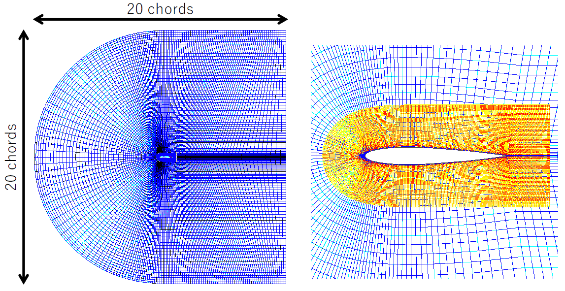
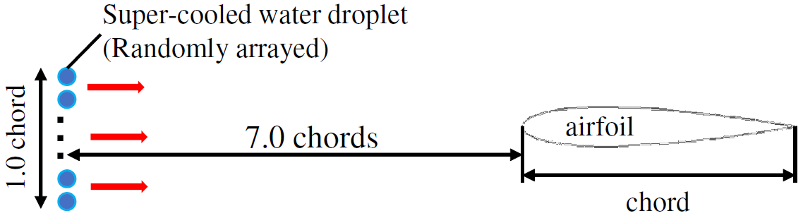
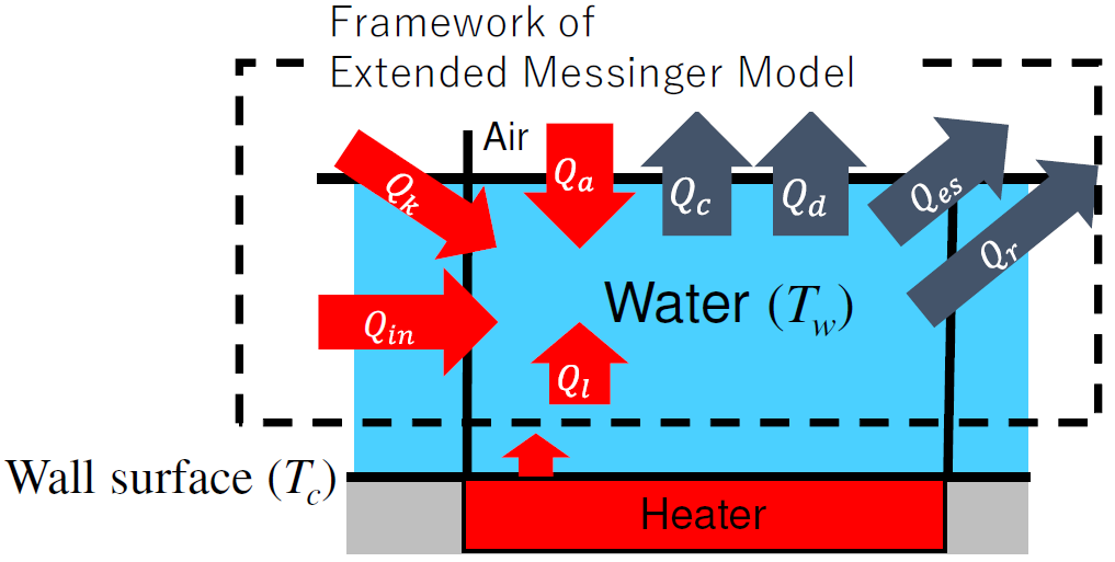
2.1. Numerical Procedure

We perform two-dimensional icing simulations for the HAARP-II and NACA0012 airfoils: the former is performed to validate our computational code and is discussed in the next subsection; the latter is the main focus of this study and discussed in Section 3. Numerical simulations are performed using an in-house code based on the Euler–Lagrange method. The numerical procedure is as follows. First, the computational grid is generated. Second, flow field, droplet trajectories, and thermodynamics are computed. Third, the computational grid for the iced airfoil shape is regenerated. Finally, the aerodynamic performance is determined. We note that the computational grid is regenerated without smoothing the ice shape because smoothing affects the icing location. The numerical procedure is explained in detail in a previous paper by the authors of this paper [29]; nonetheless, here we provide a brief outline of it as follows.

We consider main and sub grids as shown in Figure 1. The main grid is used to obtain the flow field, and sub grids with a fine mesh are used to accurately determine the ice shape and the boundary layer of the airfoil. After checking the grid-dependency of the solutions, the number of points of the main and sub-grids are set to $221\times 71$ and $501\times 51$, respectively, amounting to a total of approximately $41,000$ grid points. The computational grid points are the same for both the HAARP-II and NACA0012 airfoil cases. The grids are overset C-type grid systems and are obtained by Hermite polynomials [30]. For the validation of the HAARP-II case in Section 2.2, the computational grids were generated by the transfinite interpolation and elliptical–hyperbolic differential equations because of the complex ice shape. The physical values between the main and sub grids are exchanged using the Lagrangian interpolation method. The height of the first grid point from the airfoil surface is 20–80 for the sub grid and 30–300 for the main grid in wall units, except for the region around the stagnation point.

We used the RANS solver for a two-dimensional, compressible, fully turbulent flow to compute the flow field. The governing equations are the continuity, Navier–Stokes, energy, and transport equations with turbulent kinetic energy k and dissipation $\epsilon$. The Kato–Launder k-$\epsilon$ turbulent model [31] with a wall function is employed. The turbulence model can suppress the overproduction of turbulent eddy viscosity around the leading edge of the airfoil. The second-order upwind total variation diminishing (TVD) scheme [32] is employed for the inviscid terms, the second-order central difference scheme is employed for the viscous terms, and the lower upper-alternating direction implicit (LU-ADI) scheme [33] is employed for time integration.

A one-way coupling method is used, i.e., the flow field affects the trajectory of the droplet, while floating of the droplet does not affect the flow field. The size and concentration of droplets are assumed to be sufficiently small, and we do not consider collision, splitting, deformation, and rotation of the droplets. The Schiller model [34] is employed to determine the drag coefficient for a single profile $C_D$, as follows:

$$\begin{array}{c}\hfill C_D=\frac{24}{R{e}_d}\left(1+0.15R{e}_d^{0.687}\right).\end{array}$$

(1)

The Reynolds number of the droplet $R{e}_d$ is based on the diameter of the droplet $d_d$, the relative velocity between the droplet and the surrounding flow $U_r$, the density of the fluid ${\rho }_f$, and the viscosity of the fluid ${\mu }_f$. The trajectory of the particle is tracked by the Lagrangian approach and governed by a simplified Basset–Boussinesq–Oseen (BBO) equation, as follows:

$$\begin{array}{c}\hfill \frac{d\overrightarrow{U_p}}{dt}=\frac{3}{4}{C}_D\frac{{\rho }_g}{{\rho }_d}\frac{1}{d_d}\overrightarrow{U_r}\left|\overrightarrow{U_r}\right|.\end{array}$$

(2)

Here, $\overrightarrow{U_p}$ is the droplet velocity, and ${\rho }_g$ and ${\rho }_d$ are the densities of the gas (air) and droplet, respectively. Figure 2 shows the initial conditions of a droplet. The droplet is randomly installed upstream at a $7.0$ chord length and a $1.0$ chord width. The initial velocity of the droplet is the same as the inlet velocity of the uniform flow.

The ice growth is computed considering the concept of the EMM [12], which is a weak coupling method, where the time scales of the flow field and icing are significantly different. The EMM is based on the mass and energy conservation laws of the ice and water layers and the equation of phase change at the interface between ice and water. While the temperature profile is not calculated explicitly, the heat transfer is computed to assume a linear profile of temperature for ice and water layers. The concept of the EMM is explained in Figure 3. The heat balance is controlled by four heat intake values (i.e., aerodynamic heating $Q_a$, the kinetic energy of incoming droplets $Q_k$, heat brought in by runback $Q_{in}$, and latent heat release $Q_l$) and four heat release values (convection $Q_c$, cooling by the incoming droplets $Q_d$, evaporation and sublimation $Q_{es}$, and radiation $Q_r$). The ambient temperature $T_{air}$ and freezing temperature $T_f$ are considered as the temperatures of the wall surface and water film, respectively. Whether the ice formed is rime ice or glaze ice is determined by the balance of heat in the cell, and the thickness of the ice formed is estimated by the density of each type of ice. Note that rime ice and glaze ice have different densities (880 (kg/m${}^3$) and 917 (kg/m${}^3$) [12], respectively) owing to the amount of air involved.

In this study, we imposed the surface temperature $T_c$ on the heating surface, where $T_c=T_{air}$ for the case without the heating surface. The mean water temperature $T_w$ on the heating surface is estimated by assuming a linear temperature profile from the wall surface temperature $T_c$ and the balance between the heat flux in the computational cell, which is based on EMM, and is defined as follows:

$$\begin{array}{c}\hfill T_w=T_c+\frac{B_w}{2}\frac{\left(Q_a+Q_k+Q_{in}\right)-\left(Q_c+Q_d+Q_{es}+Q_r\right)}{k_w},\end{array}$$

(3)

where $B_w$ and $k_w$ are the film thickness and thermal conductivity of the water, respectively. The heat received by runback water $Q_{in}$ is estimated using the water temperature at the neighboring upstream cell $T_w^{up}$, expressed as

$$\begin{array}{c}\hfill Q_{in}={\dot{m}}_{in}{C}_w(T_w^{up}-T_c).\end{array}$$

(4)

When $T_c$ is lower than the freezing point $T_f$ (i.e., for the surface without a heater), icing occurs and the EMM is used to compute the growth of the ice layer. In addition, the temperature of the runback water is assumed to be equal to the freezing point as referred to in the EMM.

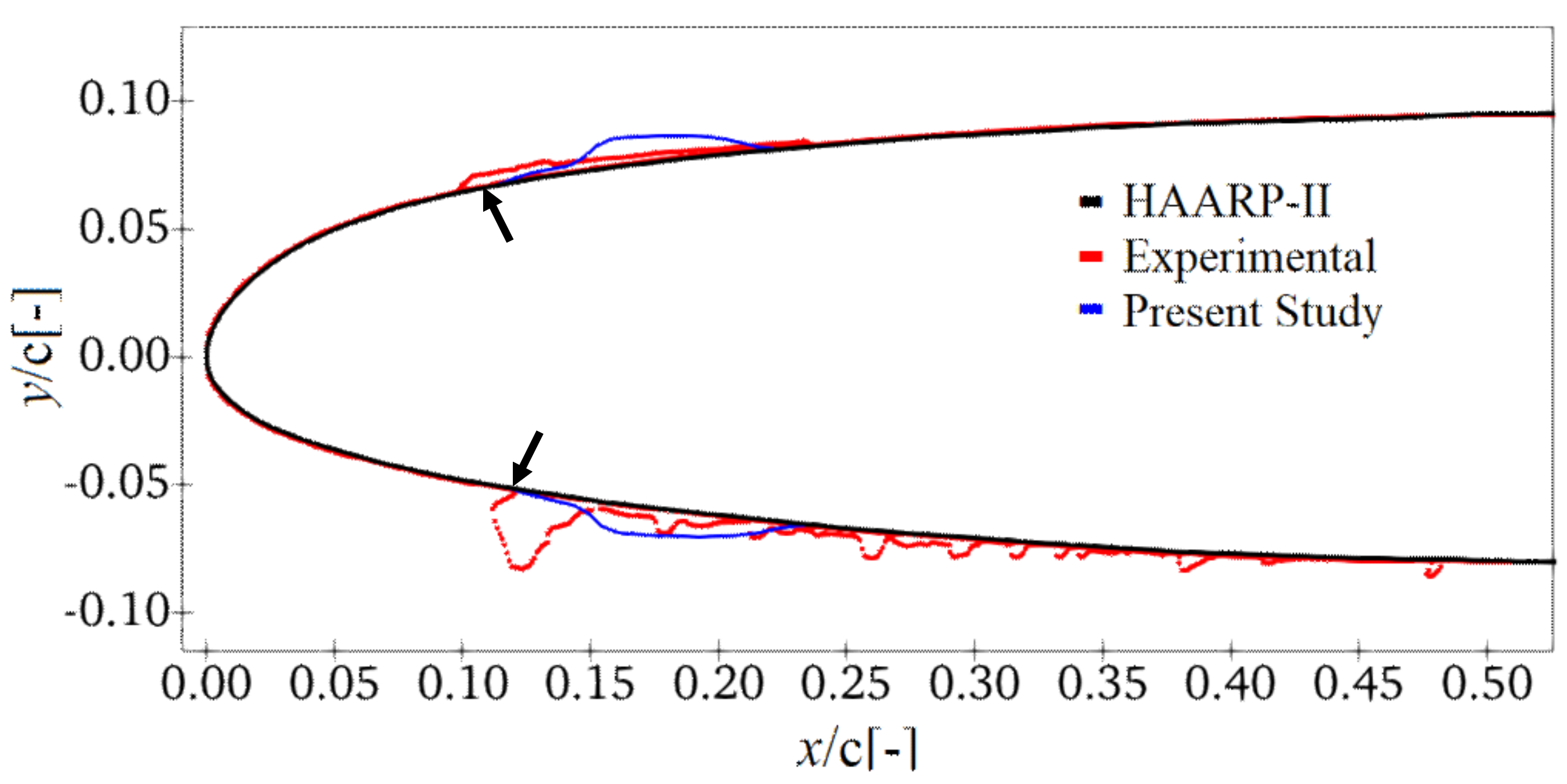
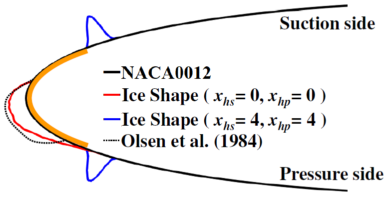
2.2. Validation for HAARP-II Airfoil

To validate the icing simulation, we compared the simulation of the HAARP-II airfoil with the experimental data by Papadaikis et al. [35]. They performed an experimental study of icing with a heated surface using bleed air for the airfoil and measured the ice shape and the surface temperature. The bleed air is installed inside the wing, near the leading edge, and it flows along the inner wall to about 10% of the chord length. The present simulation follows the experiment, and the numerical conditions are listed in

Table 1. Numerical conditions in the icing simulation for the HAARP-II airfoil. The condition follows the experiments by Papadaikis et al. [35].

Airfoil		HAARP-II
Chord length	(m)	1.524
Attack angle	(deg.)	3.0
Inlet flow velocity	(m/s)	59.2
Static temperature	(${}^{\circ }$C)	$-6.7$
MVD	($\mathsf{\mu }$m)	29
LWC	(g/m${}^3$)	0.87
Exposure time	(s)	1350

. We note that the outside surface temperature of the airfoil was set to correspond to the experimental results.

Figure 4 shows the ice shape obtained by the present simulation along with the experiment [35]. The icing starts around the leading edge on the suction side, and the locations between the simulation and experiment correspond well. Because the iced region by the simulation is similar to the region in the experiment and the deviation of the ice amount is approximately 10%, the ice shape is reasonably reproduced. In contrast, on the pressure side, although the starting location of the icing corresponds well, the iced region is significantly smaller than that in the experiment. The experiment demonstrates the large bump downstream pf the starting location and the discontinuous ice shape. Thus, a multi-shot simulation is required, the latter owing to the three-dimensionality of the icing phenomenon. The present simulation underestimates the ice shape on the pressure side because the two-dimensional and single-shot simulations are performed. In summary, the ice shape and amount on the suction side and the icing starting location on the pressure side show reasonable agreement with the experiment. Therefore, we confirmed that the present simulation can be adopted for the NACA0012 airfoil with an anti-icing system via surface heating.

3. Results and Discussion

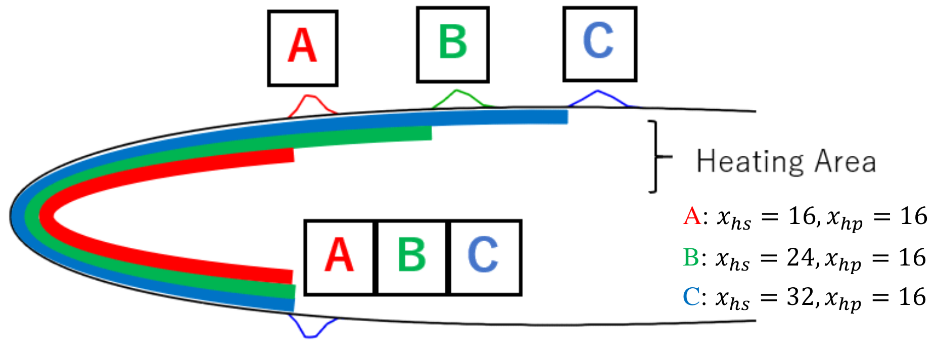
3.1. Computational Condition

We performed the icing simulation for the NACA0012 airfoil to investigate the heating effect on the ice shape and the aerodynamic performance.

Table 2. Numerical conditions for the NACA0012 airfoil (Olsen et al. [36]).

Airfoil		NACA0012
Chord length	(m)	0.53
Attack angle	(deg.)	4.0
Inlet flow velocity	(m/s)	58.1
Static temperature	(${}^{\circ }$C)	$-26$
MVD	($\mathsf{\mu }$m)	12
LWC	(g/m${}^3$)	1.08
Exposure time	(s)	300
Heating surface temperature	(${}^{\circ }$C)	10

shows the numerical conditions, which are under the glaze ice condition without heating because the static temperature is less than $-10{}^{\circ }$C. The conditions follow those in the experimental study by Olsen et al. [36].

We provide the heating area around the leading edge. The left panel of Figure 5 shows an example of the heating area: the heating area is from $x_{hs}=4\%$ to $x_{hp}=3\%$ along the surface of the airfoil, where $x_{hs}$ and $x_{hp}$ indicate the heating area on the suction and pressure sides, respectively, projected on the chordwise coordinate. In this study, the heating area is systematically changed at $0\%\le x_{hs}\le 32\%$ every 2% and $0\%\le x_{hp}\le 28\%$ every 4%. The parametric study is summarized in the map, which is explained in the right panel. The horizontal and vertical axes are $x_{hs}$ and $x_{hp}$, respectively, and the diagonal line corresponds to the symmetric heating case.

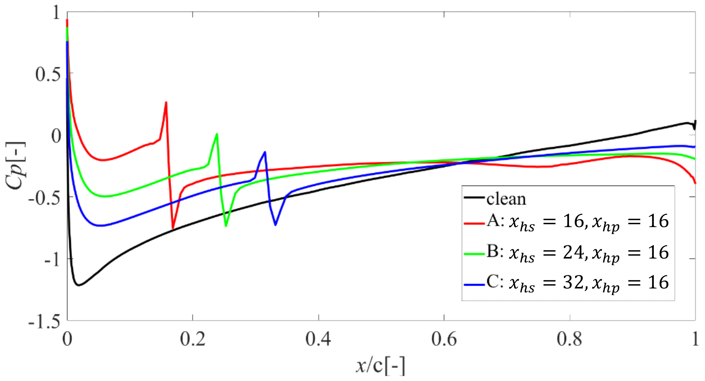
3.2. Anti-Icing and Aerodynamic Performance

The heating effect for the NACAC0012 airfoil is evaluated by the amount of adhering ice, the drag coefficient, and the lift coefficient. First, the amount of adhered ice is evaluated by the reduction rate of the ice volume. Figure 6 displays the reduction rate $\eta$, defined as

$$\begin{array}{ccc}\hfill \eta & =& 1-\frac{V}{V_0},\hfill \end{array}$$

(5)

where V is the volume of the ice for the heated case and $V_0$ means the unheated case (i.e., $x_{hs}=0$ and $x_{hp}=0$). The reduction and increase in the ice volume correspond to $\eta >0$ and $\eta <0$, respectively. The reduction rate $\eta$ is positive except for the horizontal axis of $x_{hs}=0$ and is almost constant at $\eta \approx 0.16$ in the region of $x_{hs}>4$ and $x_{hp}>4$. This is due to the following reasons. The distribution of impinging mass $m_{im}$ of the droplets is consistent for all cases because the heating does not affect the droplet trajectory computation. Therefore, the difference between cases with and without heating appears in the formed ice phases and the evaporation/sublimation $Q_{es}$. The former occurs because the runback water warmed up by the heater forms glaze ice which is $4.2$% larger in density in comparison to rime ice, indicating the reduction in the formed ice volume. The latter $Q_{es}$ is dependent on both the heat transfer coefficient as a function of wall friction and the temperature difference between the airfoil surface $T_c$ and the external edge of the boundary layer. Therefore, the evaporation and sublimation reduce the runback water by expanding the heater area near the leading edge. In contrast, apart from the leading edge, the amount of water evaporation and sublimation decreases downstream, accompanied by the decrease in wall friction. Therefore, the runback water remains downstream apart from on the leading edge. As a result, expanding the heater in the region of $x_{hs}<4$ and $x_{hp}<4$ significantly reduces the ice mass, while the runback water remains for further expanded heating cases.

Second, the drag coefficient of the airfoil is evaluated. Figure 7 shows the drag coefficient normalized by the coefficient of the clean airfoil, $C_d^{*}$. Because $C_d^{*}$ is more higher than one, the drag increases for all cases. The maximum $C_d^{*}$ is observed at $x_{hs}=4$ and $x_{hp}=4$. Roughly speaking, $C_d^{*}$ is dependent on $x_{hs}$ rather than $x_{hp}$: $C_d^{*}$ rapidly decreases as $x_{hs}$ increases, while it almost remains unchanged as $x_{hp}$ increases.

Third, Figure 8 shows the lift coefficient normalized by that of the clean airfoil, $C_l^{*}$. For all the cases, $C_l^{*}$ is less than one, and the lift coefficient decreases through the icing regardless of the heating. Moreover, $C_l^{*}$ is maximized in the unheated case of $x_{hs}=0$ and $x_{hp}=0$, which means that the lift deteriorates by heating. In addition, the lift coefficient depends on $x_{hs}$ rather than $x_{hp}$ at $x_{hp}>10$, which means the heating on the suction side is more significant than that on the pressure side.

According to the parametric study, the ice volume is reduced by the heating, and the aerodynamic performance does not improve, even in the asymmetric heating. In the following, we investigate the ice shape to discuss the deterioration by the heating and its effect on the flow field.

Figure 9 shows the ice shapes. In the unheated case ($x_{hs}=0$ and $x_{hp}=0$), the icing occurs around the leading edge, where the round shape ice forms. In the heating case ($x_{hs}=4$ and $x_{hp}=4$), the icing does not occur around the leading edge, whereas the bump-like ice forms where the heating area ends, on both the suction and pressure sides. The heater prevents icing on itself, and the runback water creates bump-like ice. Although both the round and bump shape ice induce flow separation, the influence of the bump shape is more significant, and the aerodynamics performance deteriorates as shown in Figure 7 and Figure 8. In addition, we confirmed a reasonable agreement of the ice shape between the present simulation and the experiment [36]. The bump shape was confirmed against our previous study [29] by a high-resolution simulation in the chordwise direction and by thermodynamics computation improvement.

Figure 10 shows the streamline around the airfoil in the heating case of $x_{hs}=16$ and $x_{hp}=16$. The flow separation is observed downstream of the bump ice on both sides, and it is significant on the suction side. The asymmetry of the flow separation between both sides is owing to the attack angle of ${4.0}^{\circ }$. Moreover, because of the attack angle, the flow over the suction side is significantly affected by the bump ice, and the flow separation is enlarged. The bump ice on the pressure side induces flow separation, while the separation region is small and unchanged regardless of the position of the bump ice. Therefore, the heating area on the suction side is expected to affect the aerodynamic performance significantly, whereas on the pressure side it is not. In addition, if the heating area on the suction side expands, the flow separation may shrink, resulting in the recovery of the aerodynamic performance.

Figure 11 compares the ice shape for three different cases of the heating area on the suction side: Case A, $x_{hs}=16$ and $x_{hp}=16$; Case B, $x_{hs}=24$ and $x_{hp}=16$; Case C, $x_{hs}=32$ and $x_{hp}=16$. The heating area on the suction side is extended $1.5$ times or doubled, while on the pressure side it is unchanged. As $x_{hs}$ increases, the bump ice on the suction side moves in the downstream direction, and it slightly deforms to become flatter; however, the volume is almost unchanged. They are consistent with Figure 6, Figure 7 and Figure 8, that is $\eta$ is unchanged, $C_d^{*}$ decreases, and $C_l^{*}$ recovers as $x_{hs}$ increases. The local pressure coefficient $C_p$ on the suction surface is shown in Figure 12. In the clean airfoil, $C_p$ decreases near the leading edge and recovers in the downstream direction. In the heating cases, $C_p$ is discontinuous where the bump ice is created. At the windward and leeward sides of the bump, $C_p$ increases and decreases, respectively, resulting in a decrease in lift and an increase in drag. The pressure coefficient downstream of the ice almost plateaus in the region of the flow separation.

4. Conclusions

This study shows the icing simulation for the airfoil with surface heating around the leading edge. The heater aims to prevent icing and improve the aerodynamic performance, and the heating area is asymmetrical on both sides. To focus on the anti-icing effect and aerodynamic performance of the airfoil, we assume a constant temperature at the heating area. The icing simulations of the HAARP-II and NACA0012 airfoils are numerically validated by comparing their results with the experimental data.

For the NACA0012 airfoil, the heating effect around the leading edge on the ice shape and aerodynamic performance is investigated. The ice volume decreased by expanding the heater area, except in the case with heating only on the pressure surface. The volume is almost unchanged by further extending the heating area for the 4% chord location. However, the aerodynamic performance of $C_d^{*}$ and $C_l^{*}$ deteriorates owing to the heating because an bump ice is created at the end of the heating area. The bump ice is created because of the runback flow generated by the heater, while it generates the flow separation. Because the airfoil has the attack angle, the influence of the bump ice on the suction side is significant. Therefore, we can conclude that it is somewhat difficult to improve the aerodynamic performance via partial heating around the leading edge.

References

1. Petty, K.R.; Floyd, C.D. A statistical review of aviation airframe icing accidents in the US. In Proceedings of the 11th Conference on Aviation, Range, and Aerospace, Hyannis, MA, USA, 7 October 2004. [Google Scholar]
2. Jeck, R.K. Icing Design Envelopes (14 CFR Parts 25 and 29, Appenddix C) Converted to a Distance-Based Format; Technical Report; Federal Aviation Administration Technical Center: Atlantic City, NJ, USA, 2002. [Google Scholar]
3. Mason, J. Engine power loss in ice crystal conditions. Aero Quartely 2007, 4, 12–17. [Google Scholar]
4. Beaugendre, H.; Morency, F.; Habashi, W.G. FENSAP-ICE’s three-dimensional in-flight ice accretion module: ICE3D. J. Aircr. 2003, 40, 239–247. [Google Scholar] [CrossRef]
5. Villedieu, P.; Trontin, P.; Guffond, D.; Bobo, D. SLD Lagrangian modeling and capability assessment in the frame of ONERA 3D icing suite. In Proceedings of the 4th AIAA Atmospheric and Space Environments Conference, New Orleans, LA, USA, 25–28 January 2012; p. 3132. [Google Scholar]
6. Alekseyenko, S.; Sinapius, M.; Schulz, M.; Prykhodko, O. Interaction of Supercooled Large Droplets with Aerodynamic Profile; Technical Report; SAE Technical Paper: Warrendale, PA, USA, 2015. [Google Scholar]
7. Takahashi, T.; Fukudome, K.; Mamori, H.; Fukushima, N.; Yamamoto, M. Effect of Characteristic Phenomena and Temperature on Super-Cooled Large Droplet Icing on NACA0012 Airfoil and Axial Fan Blade. Aerospace 2020, 7, 92. [Google Scholar] [CrossRef]
8. Bae, J.; Yee, K. Numerical Investigation of Droplet Breakup Effects on Droplet–Wall Interactions Under SLD Conditions. Int. J. Aeronaut. Space Sci. 2001, 22, 1005–1018. [Google Scholar] [CrossRef]
9. Messinger, B.L. Equilibrium temperature of an unheated icing surface as a function of air speed. J. Aeronaut. Sci. 1953, 20, 29–42. [Google Scholar] [CrossRef]
10. Myers, T.G. Extension to the Messinger model for aircraft icing. AIAA J. 2001, 39, 211–218. [Google Scholar] [CrossRef] [Green Version]
11. Myers, T.; Charpin, J.; Thompson, C. Slowly accreting ice due to supercooled water impacting on a cold surface. Phys. Fluids 2002, 14, 240–256. [Google Scholar] [CrossRef]
12. Özgen, S.; Canıbek, M. Ice accretion simulation on multi-element airfoils using extended Messinger model. Heat Mass Transf. 2009, 45, 305. [Google Scholar] [CrossRef]
13. Iwago, M.; Fukudome, K.; Mamori, H.; Fukushima, N.; Yamamoto, M. Fundamental investigation to predict ice crystal icing in jet engine. Recent Asian Res. Therm. Fluid Sci. 2020, 305–318. [Google Scholar]
14. Linton, A. Ice Protection System. US Patent 6848656, 2005. [Google Scholar]
15. Hannat, R.; Morency, F. Numerical validation of conjugate heat transfer method for anti-/de-icing piccolo system. J. Aircr. 2014, 51, 104–116. [Google Scholar] [CrossRef]
16. Addy, H.E.; Oleskiw, M.; Broeren, A.P.; Orchard, D. A study of the effects of altitude on thermal ice protection system performance. In Proceedings of the 5th AIAA Atmospheric and Space Environments Conference, San Diego, CA, USA, 24–27 June 2013; p. 2934. [Google Scholar]
17. Loughborough, D.L.; Green, H.E.; Roush, P.A. A Study of Wing De-Icer Performance on Mount Washington. Aero. Eng. Rev 1948, 7, 41–50. [Google Scholar]
18. D’Avirro, J.; Chaput, M.D. Optimizing the Use of Aircraft Deicing and Anti-Icing Fluids; Transportation Research Board: Washington, DC, USA, 2011; Volume 45. [Google Scholar]
19. Sulej, A.M.; Polkowska, Ż.; Astel, A.; Namieśnik, J. Analytical procedures for the determination of fuel combustion products, anti-corrosive compounds, and de-icing compounds in airport runoff water samples. Talanta 2013, 117, 158–167. [Google Scholar] [CrossRef]
20. Al-Khalil, K.M.; Horvath, C.; Miller, D.R.; Wright, W.B. Validation of NASA Thermal Ice Protection Computer Codes. Part 3; The Validation of Antice. In Proceedings of the 35th Aerospace Sciences Meeting and Exhibit, Reno, NV, USA, 6–9 January 1997. [Google Scholar]
21. Harireche, O.; Verdin, P.; Thompson, C.P.; Hammond, D.W. Explicit finite volume modeling of aircraft anti-icing and de-icing. J. Aircr. 2008, 45, 1924–1936. [Google Scholar] [CrossRef]
22. Reid, T.; Baruzzi, G.S.; Habashi, W.G. FENSAP-ICE: Unsteady conjugate heat transfer simulation of electrothermal de-icing. J. Aircr. 2012, 49, 1101–1109. [Google Scholar] [CrossRef]
23. Bu, X.; Lin, G.; Yu, J.; Yang, S.; Song, X. Numerical simulation of an airfoil electrothermal anti-icing system. Proc. Inst. Mech. Eng. Part G J. Aerosp. Eng. 2013, 227, 1608–1622. [Google Scholar] [CrossRef]
24. Lei, G.; Dong, W.; Zhu, J.; Zheng, M. Numerical Investigation of the Electrothermal De-Icing Process of a Rotor Blade; Technical Report; SAE Technical Paper: Warrendale, PA, USA, 2015. [Google Scholar]
25. Mu, Z.; Lin, G.; Shen, X.; Bu, X.; Zhou, Y. Numerical simulation of unsteady conjugate heat transfer of electrothermal deicing process. Int. J. Aerosp. Eng. 2018, 2018, 5362541. [Google Scholar] [CrossRef]
26. Asaumi, N.; Mizuno, M.; Tomioka, Y.; Suzuki, K.; Hyugaji, T.; Kimura, S. Experimental Investigation and Simple Estimation of Heat Requirement for Anti-Icing. J. Gas Turbine Soc. Jpn. 2018, 46, 476–485. (In Japanese) [Google Scholar]
27. Shen, X.; Guo, Q.; Lin, G.; Zeng, Y.; Hu, Z. Study on loose-coupling methods for aircraft thermal anti-Icing system. Energies 2020, 13, 1463. [Google Scholar] [CrossRef] [Green Version]
28. Zhou, W.; Liu, Y.; Hu, H.; Hu, H.; Meng, X. Utilization of thermal effect induced by plasma generation for aircraft icing mitigation. AIAA J. 2018, 56, 1097–1104. [Google Scholar] [CrossRef]
29. Uranai, S.; Fukudome, K.; Mamori, H.; Fukushima, N.; Yamamoto, M. Numerical Simulation of the Anti-Icing Performance of Electric Heaters for Icing on the NACA 0012 Airfoil. Aerospace 2020, 7, 123. [Google Scholar] [CrossRef]
30. Chung, T. Computational Fluid Dynamics; Cambridge University Press: Cambridge, UK, 2010. [Google Scholar]
31. Kato, M. The modelling of turbulent flow around stationary and vibrating square cylinders. Turbul. Shear. Flow 1993, 1, 10.4.1–10.4.6. [Google Scholar]
32. Yee, H.C. Upwind and Symmetric Shock-Capturing Schemes; NASA-TM-89464; NASA: Washington, DC, USA, 1987. [Google Scholar]
33. Fujii, K.; Obayashi, S. Practical applications of new LU-ADI scheme for the three-dimensional Navier-Stokes computation of transonic viscous flows. In Proceedings of the 24th Aerospace Sciences Meeting, Reno, NV, USA, 6–9 January 1986; p. 513. [Google Scholar]
34. Schiller, L.; Naumann, A. A drag coefficient correlation. Vdi Ztg. 1935, 77, 318–320. [Google Scholar]
35. Papadakis, M.; Wong, S.H.; Yeong, H.W.; Wong, S.C.; Vu, G. Icing tunnel experiments with a hot air anti-icing system. In Proceedings of the 46th AIAA Aerospace Sciences Meeting and Exhibit, Reno, NV, USA, 7–10 January 2008; p. 444. [Google Scholar]
36. Olsen, W.; Shaw, R.; Newton, J. Ice shapes and the resulting drag increase for a NACA 0012 airfoil. In Proceedings of the 22nd Aerospace Sciences Meeting, Reno, NV, USA, 9–12 January 1984; p. 109. [Google Scholar]
Figure 1. Computational grid for NACA0012. The left and right figures depict overall and enlarged views around the airfoil, respectively. The black and blue lines indicate the main and sub grids, respectively.
Aerospace 08 00294 g001
Figure 2. Schematics of droplet input.
Aerospace 08 00294 g002
Figure 3. Concept of the thermodynamic model based on the energy balance in a computational cell. The energies into and out of the cell are indicated by the red and dark blue arrows, respectively.
Aerospace 08 00294 g003
Figure 4. Ice shape for HAARP-II with experiment the by Papadaikis et al. [35]. Red and blue lines represent experimental and the present results, respectively. Arrows represent the icing starting location.
Aerospace 08 00294 g004
Figure 5. Left, heating area around the leading edge surface location; right, explanation of results map (red lines in the small figures are the heating surface).
Aerospace 08 00294 g005
Figure 6. Ice volume reduction η . The plus symbol represents a single simulation.
Aerospace 08 00294 g006
Figure 7. Drag coefficient change C d * . The plus symbol represents a single simulation.
Aerospace 08 00294 g007
Figure 8. Lift coefficient change C l * . The plus symbol represents a single simulation.
Aerospace 08 00294 g008
Figure 9. Formed ice shapes with and without heating. The orange bold line represents the heater location and the dot line represents Olsen’s test result [36].
Aerospace 08 00294 g009
Figure 10. Streamlines for x h s = 16 and x h p = 16 cases. Bold lines show the airfoil and light blue area represents the ice. The red line represents the heater location.
Aerospace 08 00294 g010
Figure 11. Formed ice shapes for three heating cases. Heating areas are displayed by the bold line with the same case index color.
Aerospace 08 00294 g011
Figure 12. Pressure coefficient on the suction surface.
Aerospace 08 00294 g012