
Tightly Coupled Integrated Navigation Algorithm for Hypersonic Boost-Glide Vehicles in the LCEF Frame


1
School of Astronautics, Northwestern Polytechnical University, Xi’an 710072, China
2
School of Electronics and Information, Northwestern Polytechnical University, Xi’an 710072, China
*
Author to whom correspondence should be addressed.
Aerospace 2021, 8(5), 124; https://0-doi-org.brum.beds.ac.uk/10.3390/aerospace8050124
Submission received: 25 February 2021
/
Revised: 12 April 2021
/
Accepted: 19 April 2021
/
Published: 23 April 2021
Abstract
:According to the trajectory characteristics of hypersonic boost-glide vehicles, a tightly coupled integrated navigation algorithm for hypersonic vehicles based on the launch-centered Earth-fixed (LCEF) frame is proposed. First, the strapdown inertial navigation mechanization algorithm and discrete update algorithm in the LCEF frame are introduced. Subsequently, the attitude, velocity, and position error equations of strapdown inertial navigation in the LCEF frame are introduced. The strapdown inertial navigation system/global positioning system (SINS/GPS) pseudo-range and pseudo-range rate measurement equations in the LCEF frame are derived. Further, the tightly coupled SINS/GPS integrated navigation filter state equation and the measurement equation are presented. Finally, the tightly coupled SINS/GPS integrated navigation algorithm is verified in the hardware-in-the-loop (HWIL) simulation environment. The simulation results indicate that the precision of tightly coupled integrated navigation is better than that of loosely coupled integrated navigation. Moreover, even when the number of effective satellites is less than four, tightly coupled integrated navigation functions well, thus verifying the effectiveness and feasibility of the algorithm.
1. Introduction
Hypersonic vehicles are being developed by various countries in the world today because of their strong strategic deterrence, air–space integrated information support, control capabilities, rapid navy, army, and air strike capabilities, and remote air interception capabilities [1]. Countries with strong economic and military capabilities such as the United States, Russia, and China have conducted a large number of flight tests, while some countries have even formally installed hypersonic missiles in their militaries [2].
The commonly used navigation systems for hypersonic vehicles include the inertial navigation system (INS), global navigation satellite system (GNSS), and celestial navigation system (CNS) [3]. The INS are self-contained and are more accurate in the short term and they can supply data continuously at a very high rate. The main drawback of an INS is the degradation of its performance with time. The GNSS receivers has high precision in long-time navigation and can bound the errors to an acceptable level. The INS and GNSS are natural complementarity. Therefore, the navigation systems of hypersonic vehicles worldwide are mainly inertial/satellite integrated navigation systems [4]. The Unites States’ X-43A hypersonic vehicle of NASA’s Hyper-X program uses a mature INS/GPS integrated navigation system [5]. The navigation system of the Hypersonic Technology Vehicle 2 (HTV-2) uses a tightly coupled INS/GPS navigation, achieving a navigation precision of up to 3 m [6]. Russia’s Avangard hypersonic missile and India’s BrahMos-II also use the INS/GNSS navigation [7].
The inertial/satellite integrated navigation system can be classified into three types based on the integration degree: loosely coupled, tightly coupled, and ultra-tightly coupled [8]. The algorithm for a loosely coupled system is relatively simple to calculate and easy to implement, and it is widely used in engineering practice. However, its navigation precision is not comparable to that of a tightly coupled system and its anti-interference ability is poor. The design of an ultra-tightly coupled system is complicated with large calculation load. Its engineering realization is limited by the development capability of satellite receivers. Tight coupling corrects the inertial navigation system through pseudo-range and pseudo-range rate satellite observations. A tightly coupled system does not require satellite receivers to provide complete positioning information and has high navigation precision. When the effective number of satellites is less than four, it can still perform integrated navigation and has strong anti-interference ability. This can meet the navigation needs of hypersonic vehicles. In recent years, scholars have increasingly studied tightly coupled INS/GNSS integrated navigation [9]. Dai et al. proposed a tightly coupled strapdown inertial navigation system/BeiDou system (SINS/BDS) algorithm based on the fast hybrid Gaussian unscented Kalman filter (UKF) algorithm. While the precision is lower than that of the traditional generalized maximum likelihood-type UKF (GM-UKF), it effectively improves the filtering calculation efficiency and the calculation speed [10]. Feng et al. used tightly coupled INS/GNSS integrated navigation technology to survey and map the surface of a shore collapsed terrain [11]. Zhao et al. studied a faster and more efficient tightly coupled SINS/GNSS navigation algorithm based on the simplified steady state KF (SSKF). Furthermore, the navigation precision is similar to that of the traditional SSKF algorithm [12]. The tightly coupled GPS/INS algorithm proposed by Yu et al. fully combines the characteristics of the aggregation constraint method and the UKF and improves the calculation efficiency [13].
As a hypersonic boost-glide vehicle has dual flight control and navigation requirements for space and aviation [4], a single launch-centered inertial (LCI) frame in space and a local-level frame in aviation cannot meet its navigation requirements simultaneously [14]. Therefore, a navigation reference frame combining the characteristics of the LCI frame and the local-level frame is needed to meet the dual requirements of space and aviation for hypersonic vehicles. The strapdown inertial navigation algorithm in the launch-centered Earth-fixed (LCEF) frame was presented in reference [4], proposing solutions to the abovementioned problems [4]. References [14,15] introduced the loosely coupled integrated navigation algorithm in the LCI frame and the LCEF frame, respectively. Based on references [4,14,15], this paper derives the tightly coupled SINS/GPS integrated navigation algorithm, KF state, and measurement equation. A solution for the tightly coupled integrated navigation of hypersonic boost-glide vehicles is proposed.
2. Strapdown Inertial Navigation Algorithm in the LCEF Frame
2.1. Coordinate System
The following coordinate systems are used in this paper and the LCEF frame is selected as the navigation reference coordinate system [4].
- The Earth-centered inertial (ECI) frame, i;
- the Earth-centered Earth-fixed (ECEF) frame, e;
- the body-fixed (BF) frame, b;
- the launch-centered Earth-fixed (LCEF) frame, g;
- the launch-centered inertial (LCI) frame, a.
2.2. Strapdown Inertial Navigation Mechanization in the LCEF Frame
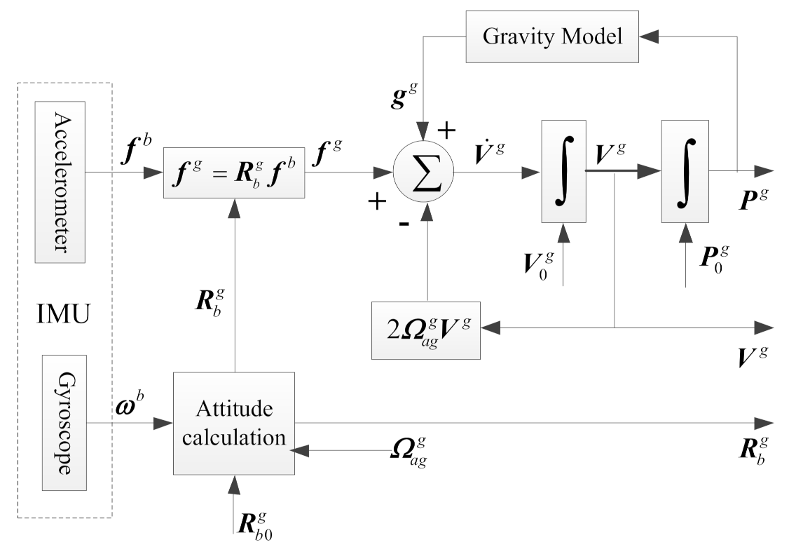
The strapdown inertial navigation equation in the LCEF frame is as follows and the mechanization is shown in Figure 1.
where represent the position, velocity, and attitude matrices of the carrier (hypersonic vehicle) in the LCEF frame, respectively, and . represents the specific force measured by the triaxial accelerometers; is the anti-symmetric matrix of the carrier relative to the rotational angular velocity ; is the gravity of the carrier in the LCEF frame; is the anti-symmetric matrix of the carrier angular velocity ; and , where is the angular velocity measured by the triaxial gyroscopes, abbreviated as .
2.3. Navigation Numerical Update Algorithm
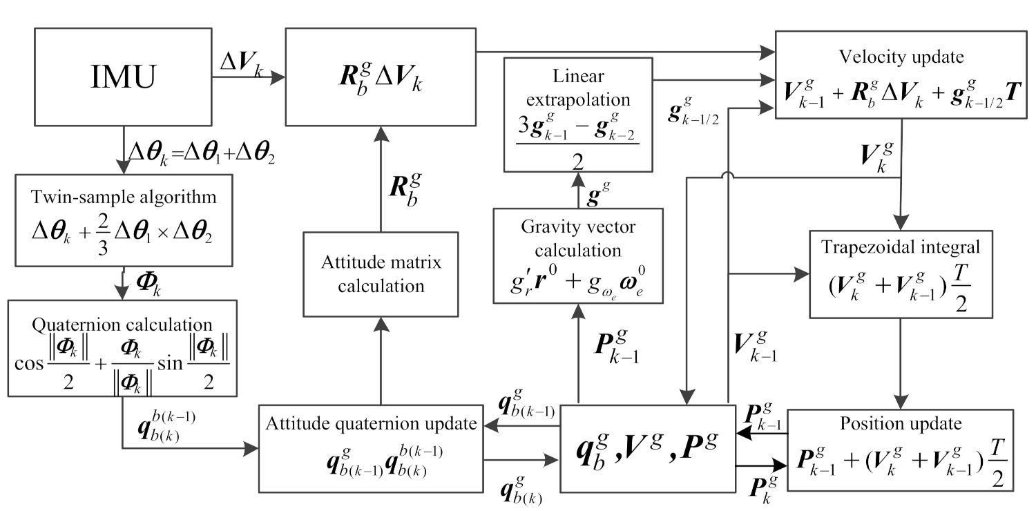
The strapdown inertial navigation algorithm in the LCEF frame consists of three parts: attitude, velocity, and position update algorithms [15]. Since this navigation numerical update algorithm has been deduced in detail in reference [15], the flow diagram of the update algorithm is presented in Figure 2.
In Figure 2, T represents the calculation cycle; are the angular increments of two equal-interval samples in a calculation cycle; are the angular increment and velocity increment of the calculation cycle, respectively; is the rotation vector; represents the attitude quaternion; and represents the gravity vector in the LCEF frame.
3. Tightly Coupled Integrated Navigation in the LCEF Frame
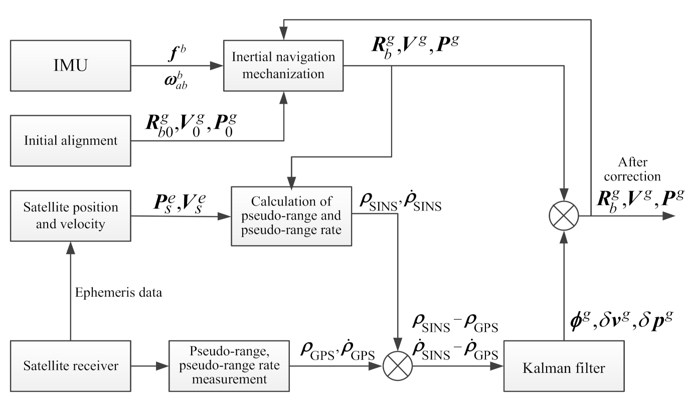
The schematic diagram of the tightly coupled SINS/GPS integrated navigation algorithm in the LCEF frame is shown in Figure 3.
3.1. SINS Error Equation in the LCEF Frame
The SINS navigation error equations in the LCEF frame include attitude, velocity, and position error equations [14]. They are obtained by linearizing the attitude, velocity, and position equations in Equation (1) with first-order small disturbances, as shown in Equation (2).
where is the anti-symmetric matrix of the specific force in the LCEF frame; is the gravity error of the carrier in the LCEF frame; and .
3.2. Tightly Coupled State Equation in the LCEF Frame
The state equation of the KF system for tightly coupled SINS/GPS is
The SINS state vector includes the attitude, velocity, position, gyroscope, and accelerometer errors in the LCEF frame [14].
The GPS state vector includes the range error and clock drift caused by satellite receiver clock deviation.
Moreover:
where and are the standard deviations of white noise of clock deviation and clock drift, respectively.
By expanding Equation (3), we obtain:
3.3. Tightly Coupled Measurement Equation in the LCEF Frame
The SINS/GPS tightly coupled KF measurement equation is:
For M visible satellites:
As shown in Equation (9), the SINS/GPS tightly coupled measurement equation is composed of pseudo-range and pseudo-range rate measurement equations, obtained through and , respectively.
3.3.1. Pseudo-Range Measurement Equation in the LCEF Frame
The pseudo-range from the carrier position to the m-th satellite calculated by the strapdown inertial navigation system is
where is the position in the ECEF frame calculated by strapdown inertial navigation, and is the position of the m-th GPS satellite in the ECEF frame.
The pseudo-range measurement equation of the m-th GPS satellite is
where is the distance error caused by clock deviation ; is the pseudo-range measurement noise, which is mainly composed of the ionospheric error, tropospheric error, and multi-path effect error; and is the position of the GPS receiver in the ECEF frame.
After the Taylor series expansion of Equation (11) and subtracting Equation (10) from it, the following can be obtained:
The line-of-sight unit vector from the m-th satellite to the carrier position calculated by SINS/GPS is defined as:
Substituting Equation (13) into Equation (12), we obtain:
where:
For M visible satellites, Equation (15) can be written as:
Define:
Substituting Equations (17)–(19) into Equation (16), we obtain:
Transforming the position in the LCEF frame to the ECEF frame, we get:
where ; is the conversion matrix from the ECEF frame to the LCEF frame, which is relevant to the initial longitude , latitude , and heading direction of the carrier, as shown in Equation (22).
Substituting Equations (21) and (22) into Equation (20), we obtain:
Define:
Substituting Equation (24) into Equation (23), the pseudo-range measurement equation can be obtained as:
3.3.2. Pseudo-Range Rate Measurement Equation in the LCEF Frame
The pseudo-range rate is modeled as:
where is the clock drift (m/s), and is the line-of-sight unit vector from the m-th satellite to the carrier, which can be represented as:
Considering the position as and substituting it in Equation (27), the following can be obtained:
Taking the derivative of Equation (10), the following can be obtained:
where is the velocity calculated by the strapdown inertial navigation in the ECEF frame, and is the velocity of the m-th satellite in the ECEF frame.
The difference between Equations (29) and (26) will give the following:
For M visible satellites, Equation (30) can be written as:
Define:
Substituting Equations (17), (32), and (33) into Equation (31), we obtain:
Transforming the velocity in the LCEF frame to the ECEF frame, we obtain:
Substituting Equation (35) into Equation (34), we obtain:
Substituting Equation (24) into Equation (36), the pseudo-range rate measurement equation can be obtained as follows:
In summary, the measurement equation of the SINS/GPS tightly coupled integrated navigation system in the LCEF frame is:
where:
4. Simulation Verification
In order to verify the accuracy and superiority of the tightly coupled SINS/GPS integrated navigation in the LCEF frame, a hardware-in-the-loop (HWIL) simulation was performed. In the HWIL system, a three-axis rotation table simulates the flight attitude, while an actuator load simulator simulates the torque of the rudder. An IMU simulator receives real-time information on the theoretical specific force from a real-time 6DOF simulator. A GPS simulator receives real-time information the 6DOF simulator [15,16].
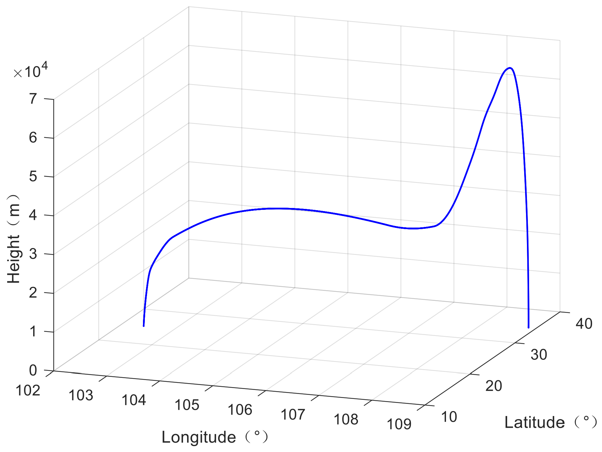
The integrated navigation results of the loosely and tightly coupled SINS/GPS in the LCEF frame were compared. In addition, the results of the tight coupling of the normal number of satellites were compared with those of the tight coupling of less than four satellites. For the simulation verification, we adopted a classic trajectory of a hypersonic vehicle with the duration of 1100 s for simulation verification [15,16]. The initial state of the trajectory was velocity 0 m/s, latitude 34.2°, longitude 108.9°, and height 400 m. In addition, the shooting direction, pitch angle, roll angle, and yaw angle were 200°, 90°, 0°, and 0°, respectively. The flight path is shown in Figure 4. Parameters of SINS/GPS integrated navigation system in the HWIL simulation are shown in Table 1.
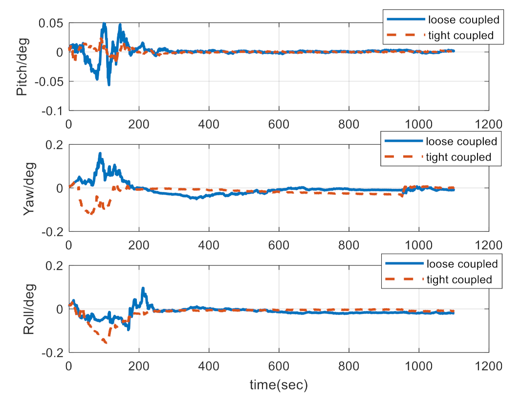
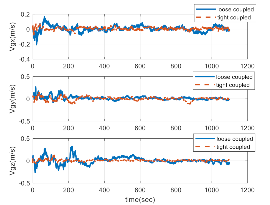
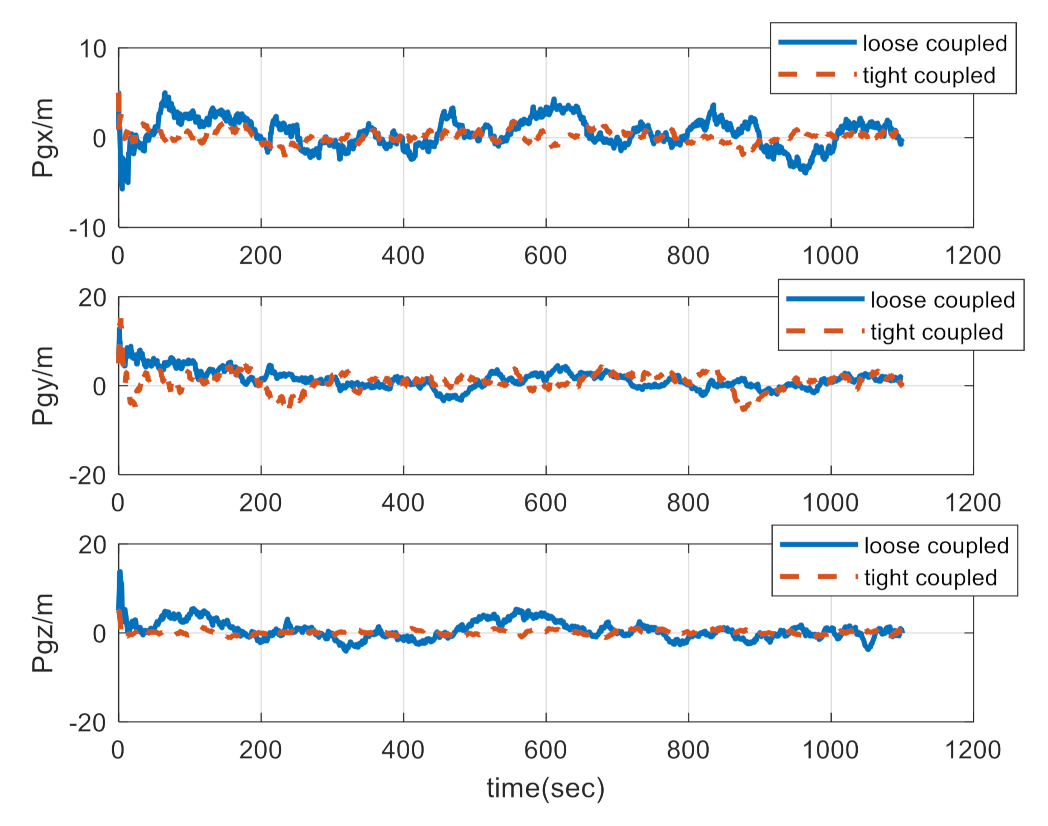
4.1. Comparison between Loose and Tight Coupling
Figure 5, Figure 6, Figure 7 show the comparison of the HWIL simulation results between loosely and tightly coupled integrated navigation in the LCEF frame. In the SINS/GPS loose coupling simulation results in the LCEF frame, the pitch angle convergence error is 0.0048°, yaw angle convergence error is 0.028°, roll angle convergence error is 0.0021°, X-axis velocity convergence error is 0.08 m/s, Y-axis velocity convergence error is 0.07 m/s, z-axis velocity error is 0.12 m/s, X-axis position convergence error is 3.6 m, Y-axis position convergence error is 4.8 m, and Z-axis position convergence error is 5.2 m. In the SINS/GPS tightly coupled simulation results in the LCEF frame, the pitch angle convergence error is 0.0043°, yaw angle convergence error is 0.012°, roll angle convergence error is 0.0029°, X-axis velocity convergence error is 0.03 m/s, Y-axis velocity convergence error is 0.11 m/s, z-axis velocity convergence error is 0.06 m/s, X-axis position convergence error is 1.2 m, Y-axis position convergence error is 4.9 m, and Z-axis position convergence error is 4.9 m. Overall, the precision of the tightly coupled navigation system is better than that of the loosely coupled navigation system.
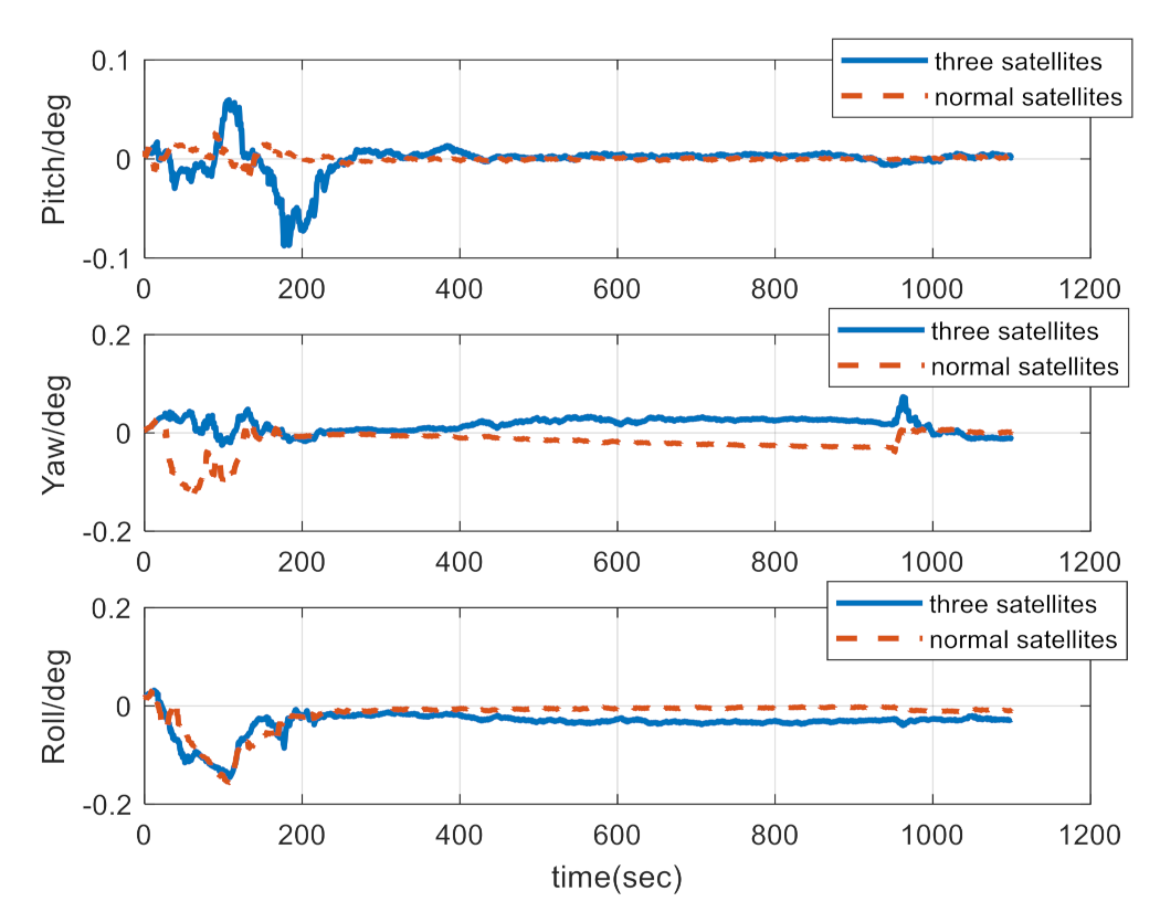
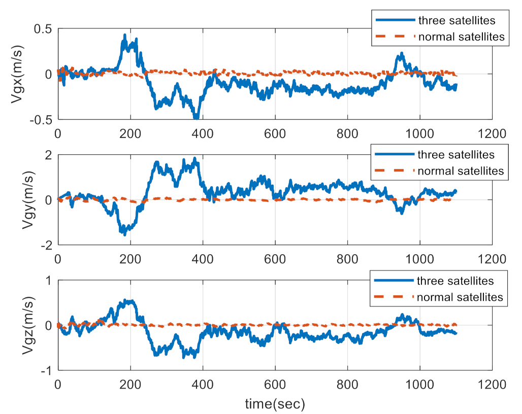
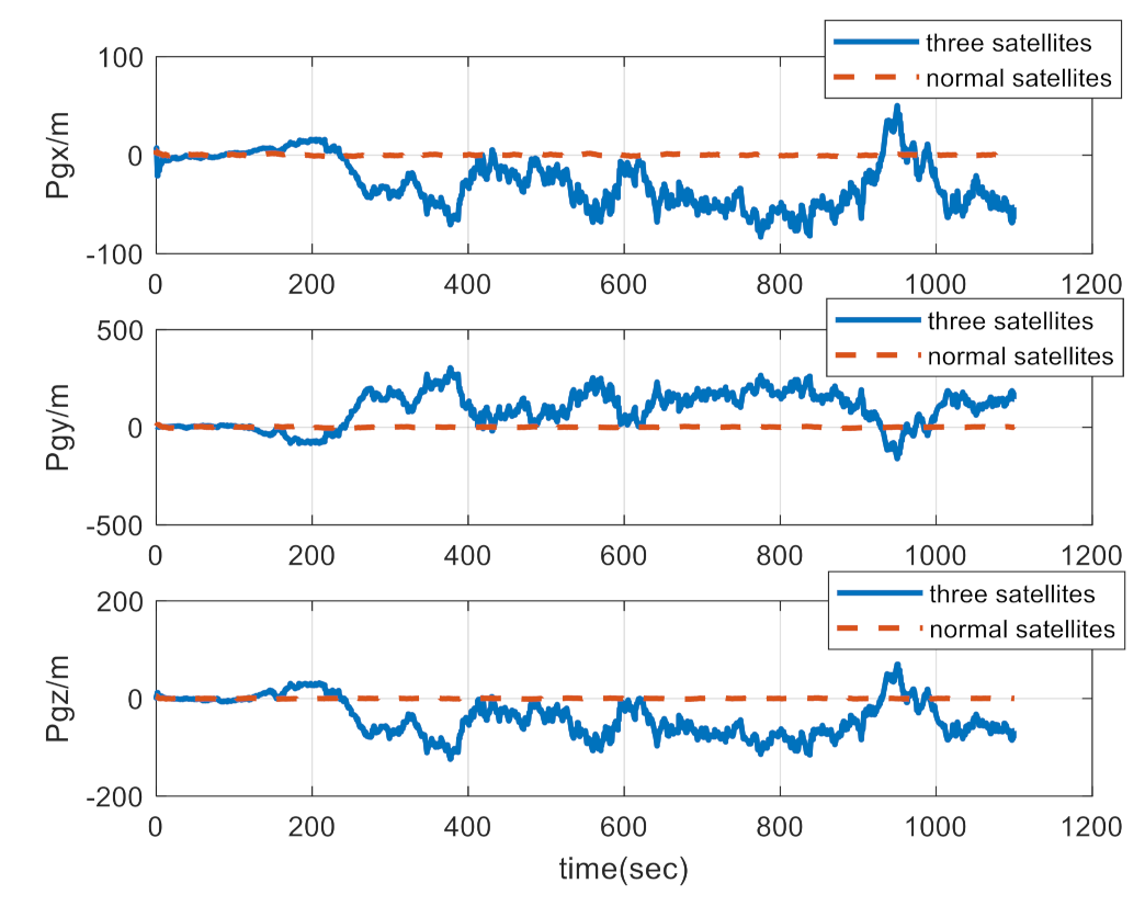
4.2. Navigation Comparison between the Normal-Number Satellite and Three-Satellite Integrated Navigation
Figure 8, Figure 9, Figure 10 show the result of the comparison of a SINS/GPS tightly coupled normal-number satellite and three-satellite integrated navigation in the LCEF frame. In the SINS/GPS tightly coupled simulation results of three effective satellites, the pitch angle convergence error is 0.012°, yaw angle convergence error is 0.034°, and roll angle convergence error is 0.029°; the maximum X-axis velocity error is 0.42 m/s, the maximum Y-axis velocity error is 0.86 m/s, and the maximum z-axis velocity error is 0.46 m/s; the maximum X-axis position error is 84 m, the maximum Y-axis position error is 213 m, and the maximum position error of z-axis is 118 m.
Overall, when adopting three satellites for navigation, the navigation precision declines while integrated navigation can still be conducted. Thus, tightly coupled navigation has great advantages compared with loosely coupled navigation.
5. Conclusions
In this paper, the strapdown inertial navigation algorithm and the tightly coupled integrated navigation algorithm of hypersonic vehicles under the LCEF frame were designed and verified by simulation. The integrated navigation system under the LCEF frame cannot be singular in the attitude angle under vertical launch conditions, which is suitable for boost-glide vehicles. The LCEF frame adopts the J2 gravity model, which is different from the normal gravity model in the local-level frame. It is suitable for near-space flying altitude of above 20 km. The digital simulation test verifies that the precision of tightly coupled navigation is better than that of loosely coupled navigation. Tightly coupled navigation functions even when the effective number of satellites is less than four; thus, the issue of vulnerability of satellite navigation to interference is overcome.
Author Contributions
Conceptualization, K.C., F.S., S.L. and S.P.; methodology, K.C. and F.S.; software, F.S.; validation, K.C. and S.P.; data curation, K.C., S.L. and S.P.; writing—original draft preparation, K.C. and S.P.; writing—review and editing, K.C., S.L. and S.P. All authors have read and agreed to the published version of the manuscript.
Funding
This work was supported by the Space Science and Technology Innovation Fund of China (2016KC020028) and the Fund of China Space science and Technology (2017-HT-XG).
Institutional Review Board Statement
Not applicable.
Informed Consent Statement
Not applicable.
Data Availability Statement
The programs are not publicly available, due to a part of simulation programs in use, but are available from the corresponding author on reasonable request.
Conflicts of Interest
The authors declare no conflict of interest.
References
- Zhao, L.-Y.; Yong, E.-M.; Wang, B.-L. Several research advances of anti-near space hypersonic vehicle. J. Astronaut. 2020, 41, 1239–1250. [Google Scholar]
- Liu, W.; Gong, H.-H. Overview of the development history of foreign hypersonic aircraft. Aerodyn. Missile J. 2020, 3, 20–27, 59. [Google Scholar]
- Yang, Y.Q.; Zhang, C.X.; Lu, J.Z.; Zhang, H. Classification of Methods in the SINS/CNS Integration Navigation System. IEEE Access 2018, 6, 3149–3158. [Google Scholar] [CrossRef]
- Chen, K.; Shen, F.; Sun, H.; Zhou, J. Hypersonic Vehicle Navigation Algorithm in Launch Centered Earth-Fixed Frame. J. Astronaut. 2019, 40, 1212–1218. [Google Scholar]
- Bahm, C.; Baumann, E.; Martin, J.; Bose, D.; Beck, R.; Strovers, B. The X-43A Hyper-X Mach 7 Flight 2 Guidance, Navigation, and Control Overview and Flight Test Results. In Proceedings of the AIAA/CIRA 13th International Space Planes and Hypersonics Systems and Technologies Conference, Capua, Italy, 16–20 May 2005. [Google Scholar]
- David, W. Research Note to Hypersonic Boost-Glide Weapons by James M. Acton: Analysis of the Boost Phase of the HTV-2 Hypersonic Glider Tests. Sci. Glob. Secur. 2015, 23, 220–229. [Google Scholar]
- Wang, L.-P.; Zhao, S.; Jiang, C.; Guo, T. Development Trends of Foreign Hypersonic Weapons. Aerosp. Electron. Warf. 2020, 36, 61–64. [Google Scholar]
- Shen, K. Research on Tight Integrated Navigation System Based on SINS/GPS. Master’s Thesis, Nanjing University of Science and Technology, Nanjing, China, 2017. [Google Scholar]
- Zhang, H.-Y. Research on SINS/GPS Tightly Coupled Integrated Navigation of Near Space Vehicle. Master’s Thesis, Northwestern Polytechnical University, Xi’an, China, 2020. [Google Scholar]
- Dai, Q.; Sui, L.-F.; Wang, L.-X.; Zeng, T.; Tian, Y. Beidou/Inertial Navigation Fast Hybrid Gaussian UKF Algorithm. Sci. Surv. Mapp. 2018, 43, 20–25. [Google Scholar]
- Feng, G.-Z.; Liu, S.-Z.; Li, Y.; Peng, C.; Yang, X.-C.; Chen, X.-R.; Long, H. Three-dimensional integrated shore collapse monitoring technology based on GNSS/INS tight coupled. J. Yangtze River Scie. Res. Inst. 2019, 36, 94–99. [Google Scholar]
- Zhao, J.; Xu, C.-D.; Zhang, P.-F. SINS/GNSS tight coupling algorithm based on simplified SSKF. J. Syst. Eng. Electron. 2017, 39, 2529–2534. [Google Scholar]
- Yu, H.; Li, Z.; Wang, J.; Han, H. Data fusion for a GPS/INS tightly coupled positioning system with equality and inequality constraints using an aggregate constraint unscented Kalman filter. J. Spat. Sci. 2018, 65, 1–22. [Google Scholar] [CrossRef]
- Chen, K.; Shen, F.; Zhou, J.; Wu, X. SINS/BDS Integrated Navigation for Hypersonic Boost-Glide Vehicles in the Launch-Centered Inertial Frame. Math. Probl. Eng. 2020, 2020, 1–16. [Google Scholar] [CrossRef]
- Chen, K.; Zhou, J.; Shen, F.-Q.; Sun, H.-Y.; Fan, H. Hypersonic boost–glide vehicle strapdown inertial navigation system/global positioning system algorithm in a launch-centered earth-fixed frame. Aerosp. Sci. Technol. 2020, 98, 105679. [Google Scholar] [CrossRef]
- Chen, K.; Shen, F.; Zhou, J.; Wu, X. Simulation Platform for SINS/GPS Integrated Navigation System of Hypersonic Vehicles Based on Flight Mechanics. Sensors 2020, 20, 5418. [Google Scholar] [CrossRef] [PubMed]
Figure 1.
Mechanization of strapdown inertial navigation in the LCEF frame.

Figure 2.
Diagram of the strapdown inertial navigation numerical update algorithm in the LCEF frame.
Figure 2.
Diagram of the strapdown inertial navigation numerical update algorithm in the LCEF frame.

Figure 3.
Diagram of tightly coupled SINS/GPS integrated navigation algorithm in the LCEF frame.

Figure 4.
3D trajectory of a hypersonic boost-glide vehicle.

Figure 5.
Comparison of attitude errors between loose and tight coupling.

Figure 6.
Comparison of velocity errors between loose and tight coupling.

Figure 7.
Comparison of position errors between loose and tight coupling.

Figure 8.
Comparison of attitude errors between normal-number satellites and three satellites.

Figure 9.
Comparison of velocity errors between normal-number satellites and three satellites.

Figure 10.
Comparison of position errors between normal-number satellites and three satellites.


Table 1.
Parameters of SINS/GPS integrated navigation simulation.
| Simulation Parameters | Index |
|---|---|
| Gyro constant deviation/(°·h−1) | 3.0 |
| Gyro random error/(°·h−1/2) | 0.3 |
| Accelerometer constant offset/(g0) | 1 × 10⁻³ |
| White noise measured by accelerometer/(g0) | 1 × 10⁻⁴ |
| Initial attitude angle errors /(′′) | 20,5,5 |
| Initial velocity error/(m·s−1) | 0.01 |
| Initial position error/(m) | 5 |
| Satellite positioning precision/(m) | 15 |
| Satellite velocity measurement precision/(m·s−1) | 0.3 |
Publisher’s Note: MDPI stays neutral with regard to jurisdictional claims in published maps and institutional affiliations. |
© 2021 by the authors. Licensee MDPI, Basel, Switzerland. This article is an open access article distributed under the terms and conditions of the Creative Commons Attribution (CC BY) license (https://creativecommons.org/licenses/by/4.0/).
Share and Cite
MDPI and ACS Style
Chen, K.; Pei, S.; Shen, F.; Liu, S. Tightly Coupled Integrated Navigation Algorithm for Hypersonic Boost-Glide Vehicles in the LCEF Frame. Aerospace 2021, 8, 124. https://0-doi-org.brum.beds.ac.uk/10.3390/aerospace8050124
AMA Style
Chen K, Pei S, Shen F, Liu S. Tightly Coupled Integrated Navigation Algorithm for Hypersonic Boost-Glide Vehicles in the LCEF Frame. Aerospace. 2021; 8(5):124. https://0-doi-org.brum.beds.ac.uk/10.3390/aerospace8050124
Chicago/Turabian StyleChen, Kai, Sensen Pei, Fuqiang Shen, and Shangbo Liu. 2021. "Tightly Coupled Integrated Navigation Algorithm for Hypersonic Boost-Glide Vehicles in the LCEF Frame" Aerospace 8, no. 5: 124. https://0-doi-org.brum.beds.ac.uk/10.3390/aerospace8050124
Note that from the first issue of 2016, this journal uses article numbers instead of page numbers. See further details here.