A Hybrid Real/Ideal Gas Mixture Computational Framework to Capture Wave Propagation in Liquid Rocket Combustion Chamber Conditions

Abstract

The present work focuses on the development of new mathematical and numerical tools to deal with wave propagation problems in a realistic liquid rocket chamber environment. A simplified real fluid equation of state is here derived, starting from the literature. An approximate Riemann solver is then specifically derived for the selected conservation laws and primitive variables. Both the new equation of state and the new Riemann solver are embedded into an in-house one-dimensional CFD solver. The verification and validation of the new code against wave propagation problems are then performed, showing good behavior. Although such problems might be of interest for different applications, the present study is specifically oriented to the low order modeling of high-frequency combustion instability in liquid-propellant rocket engines.

1. Introduction

Recent studies have provided evidence on how the injector elements of liquid rocket engines play a central role in the thermo-, hydro-, and gas-dynamic coupling that takes place during high frequency combustion instability [1,2,3]. In particular, the commonly used shear–coaxial injector shows an attitude to cyclically accumulate and release fresh fuel pockets. Such a behavior is most likely caused by the intrinsic nature of the injectors themselves, which work with a radial density gradient in the recess area, i.e., the zone where fuel and oxidizers mix with each other. When fluctuations occur, axial pressure gradients develop inside the injectors because of their basically one-dimensional shape, and the baroclinic torque arising from the coupling of the two gradients generates vortexes in turn in the recess. Since the intensity of the pressure waves during thermo-acoustic oscillations can be strong, pressure waves coming from the chamber and traveling upstream in the injector can significantly slow the flow down. In such a case, vortexes may form, trapping pockets of fresh propellant, which struggle to flow downstream, causing an accumulation process to take place at the recess location. Afterwards, when the pressure waves return, traveling downstream, the accumulated pockets are pushed into the hot gases in the chamber where they burn, releasing heat and generating new pressure waves in turn. So, the process becomes self-sustained.

This work is mainly focused on acoustic phenomena and their correct modeling. In this sense, attention has to be paid to two major sub-models, namely, the real fluid mixture equation of state (EoS) and the proper numerical approach. For both of them, several different approaches are available in the literature, spanning from very simple to very complicated models, depending on the problem that is being dealt with.

Concerning the equation of state, the most simple way to model a real fluid mixture is to assume one cubic EoS for each species, mixing them afterwards using an ideal gas mixing rule. In particular, the use of Amagat’s mixing rule [4] seems quite promising [5]. A further complication is to assume a cubic model cast for the entire mixture. In such a way, mixing is performed by means of species interaction indexes within the EoS [6,7,8]. Such a kind of modeling drops completely any kind of idealization and is quite widespread in the acoustics community, [9,10,11,12,13]. The last step of complication consists of modeling the Helmholtz free energy. Theoretically, such an elegant formulation is the most accurate, yet also the most complicated and computationally intensive among all the others. Furthermore, it is quite recent as a formulation, so many of the needed species interaction coefficients employed in it are not yet available in the literature [14,15].

For the mentioned reasons, a cubic EoS for the entire real gas mixture is chosen as a starting point [16]; then, it is significantly simplified, as described in the following sections.

To solve the conservation laws, a finite volumes numerical approach based on an approximated Riemann solver (RS) is selected. As for the EoS, a large number of Riemann solvers is available in the literature, depending on the problem under investigation. Most of them are reported in detail in [17]. In the literature, a popular approximated RS is the Roe solver, whose original formulation [18,19] was already extended to generalized EoS by Glaister [20]. Such a solver is re-derived in the following sections in different primitive variables, with respect to the original formulation, for consistency with the primitive variables that are considered in the formulation presented here.

The paper is organized as follows. First of all, the new EoS and Riemann solver are derived. Secondly, the new EoS is verified and validated against real fluid thermodynamics. After that, the Riemann solver is verified and validated against ideal gas problems. Lastly, EoS and RS models are embedded into a one-dimensional Eulerian solver, and they are validated together against wave propagation in real fluids and in real fluid mixtures.

2. Equation of State

The thermodynamic states of the propellant in a liquid rocket engine, might be very different depending on in which part of the engine it flows, spanning through liquid, vapor, gas and super-critical states. For such a reason, different models might be used in different subsystems. This is true even when dealing with different locations within the same combustion chamber.

Staring at the combustion chamber of cryogenic liquid rocket engines, one might observe that both the fuel and oxidizer are often above their critical pressure. Concerning their temperature and density, the oxidizer is generally injected at a cryogenic temperature as it comes from the associated tank, and possibly the pump; consequently, the temperature is below its critical temperature, and the density is about that of its condensed state. On the other hand, fuel is injected in a gasified state since it comes from the cooling jacket, and its temperature is often higher than its critical value. Downstream of the mixture ignition location, the temperature becomes significantly high, and higher than the mixture critical temperature.

For the mentioned reasons, only the oxidizer is chosen to be treated as a real fluid, while fuel and combustion products are assumed to behave as ideal gases. Such an assumption allows to significantly simplify the EoS formulation.

So, starting from the original formulation by Kim et al. [16], we have the following:

$$p(\rho ,T,{\chi }_i)={\displaystyle \frac{\rho R_{u}T}{\mathfrak{w}-b\rho }}-{\displaystyle \frac{a\alpha \left(T\right){\rho }^2}{\left(\mathfrak{w}+{\delta }_1\rho b\right)\left(\mathfrak{w}+{\delta }_2\rho b\right)}}$$

(1)

where $\rho$, p, T, $\mathfrak{w}$ represent the density, pressure, temperature and molar weight of the mixture, respectively, while $R_u$ is the universal gas constant and $a\alpha \left(T\right),b,{\delta }_1,{\delta }_2$, are model parameters, reading as follows:

$$a\alpha \left(T\right):=\sum _{i=1}^N\sum _{j=1}^N{\chi }_i{\chi }_j{a}_{ij}{\alpha }_{ij}\left(T\right)\mathrm{where}{a}_{ij}{\alpha }_{ij}\left(T\right):=\sqrt{a_i{a}_j{\alpha }_i\left(T\right){\alpha }_j\left(T\right)}\left(1-{\kappa }_{ij}\right)$$

(2a)

$$b:=\sum _{i=1}^N{\chi }_i{b}_i$$

(2b)

$${\delta }_1:=\sum _{i=1}^N{\chi }_i{\delta }_{1,i},{\delta }_2:=\sum _{i=1}^N{\chi }_i{\delta }_{2,i}$$

(2c)

where ${\chi }_i$ and ${\chi }_j$ are molar fractions of species i and j. As can be seen from Equation (2), parameters ${\alpha }_i$ are temperature dependent, while parameters $a_i$ and $b_i$ are constants depending only on the species. Concerning parameters $\delta$, they are actually switches capable of making the cubic law to assume the shape of Soave–Redlich–Kwong [6] (SRK), Peng–Robinson [7] (PR) or Redlich–Kwong–Peng–Robinson [8] (RK-PR) EoSs. Each of the model parameters is shown in

Table 1. Characteristic parameters of the three EoSs. Subscript “c” stands for critical and, thus, refers to quantities evaluated at the species critical point.

Parameter	SRK [6]	PR [7]	RK-PR [8]
${\delta }_1$	1	0	$d_1+d_2{(d_3-1.168Z_c)}^{d_4}+d_5{(d_3-1.168Z_c)}^{d_6}$
${\delta }_2$	$(1-{\delta }_1)/(1+{\delta }_1)$	$(1-{\delta }_1)/(1+{\delta }_1)$	$(1-{\delta }_1)/(1+{\delta }_1)$
a	$0.42747{\displaystyle \frac{{R_u}^2{T_c}^2}{p_c}}$	$0.45724{\displaystyle \frac{{R_u}^2{T_c}^2}{p_c}}$	${\displaystyle \frac{d^2+3dy+d+3y^2-1}{{(d+3y-1)}^2}}{\displaystyle \left(\frac{{R_u}^2{T_c}^2}{p_c}\right)}$
b	$0.08664{\displaystyle \frac{R_u{T}_c}{p_c}}$	$0.07780{\displaystyle \frac{R_u{T}_c}{p_c}}$	${\displaystyle \frac{1}{d+3y-1}}{\displaystyle \left(\frac{R_u{T}_c}{p_c}\right)}$
$\alpha$	${(1+S(1-\sqrt{{\displaystyle \frac{T}{T_c}}}))}^2$	${(1+S(1-\sqrt{{\displaystyle \frac{T}{T_c}}}))}^2$	${\left({\displaystyle \frac{3}{2+T/T_c}}\right)}^k$
S	$-0.15613{\omega }^2+1.55171\omega +0.48508$	$-0.26992{\omega }^2+1.54226\omega +0.37464$	–
k	–	–	${\omega }^2(A_0+1.168A_1{Z}_c)+\omega (B_0+1.168B_1{Z}_c)+(C_0+1.168C_1{Z}_c)$
d	–	–	$(1+{\delta }_1^2)/(1+{\delta }_1)$
y	–	–	$\sqrt[3]{{\displaystyle \frac{4}{{\delta }_1+1}}}+\sqrt[3]{2({\delta }_1+1)}+1$
$d_1$	–	–	0.428363
$d_2$	–	–	18.496215
$d_3$	–	–	0.338426
$d_4$	–	–	0.66
$d_5$	–	–	789.723105
$d_6$	–	–	2.512392
$A_0$	–	–	0.0017
$A_1$	–	–	−2.4407
$B_0$	–	–	1.9681
$B_1$	–	–	7.4513
$C_0$	–	–	−2.7238
$C_1$	–	–	12.5040

.

As previously mentioned, such a formulation is further simplified in order to consider only the oxidizer species as a real fluid, while fuel and combustion product mixtures are treated as ideal ones. It has to be noted that considering a species as an ideal one means assuming that it has an extremely high critical pressure and an extremely low critical temperature with respect to the operating pressure and temperature. This condition can be expressed by setting the coefficients a and b to zero (see Table 1).

In this sense, manipulating Equations (1) and (2) yields the following:

$$p(\rho ,T,{\chi }_i)={\displaystyle \frac{\rho R_{u}T}{\mathfrak{w}-{\chi }_o{b}_o\rho }}-{\displaystyle \frac{{\chi }_o^2{a}_o{\alpha }_o\left(T\right){\rho }^2}{(\mathfrak{w}+{\delta }_1\rho {\chi }_o{b}_o)(\mathfrak{w}+{\delta }_2\rho {\chi }_o{b}_o)}}$$

(3)

where the mixture molecular weight ($\mathfrak{w}$) is expressed as follows:

$$\mathfrak{w}:=\sum _i{\chi }_i{w}_i$$

(4)

and where subscript o stands for oxidizer, while the molar fractions and molar weight of the i-th species are expressed as ${\chi }_i$ and $w_i$.

Other Thermodynamic Quantities

A complete determination of the thermodynamic quantities can be found in [21]. The general expression of internal energy (e) is the following:

$$e(\rho ,T,{\chi }_i)=e_0\left(T\right)+{\int }_0^{\rho }\left[{\displaystyle \frac{p(\rho ,T,{\chi }_i)}{{\rho }^2}}-{\displaystyle \frac{T}{{\rho }^2}}{\left(\frac{{\mathit{\partial }}_p}{{\mathit{\partial }}_T}\right)}_{\rho ,{\chi }_i}\right]\mathrm{d}\rho$$

(5)

where subscript 0 represents the ideal quantities evaluated at a sufficiently rarefied reference state, in which ideal gas assumptions hold. Its derivative with respect to temperature, namely specific heat at constant volume ($c_v$), reads as follows:

$$c_v(\rho ,T,{\chi }_i):={\left(\frac{{\mathit{\partial }}_p}{{\mathit{\partial }}_T}\right)}_{\rho ,{\chi }_i}=c_{v,0}\left(T\right)+{\int }_0^{\rho }\left[-{\displaystyle \frac{T}{{\rho }^2}}{\left(\frac{{{\mathit{\partial }}^2}_p}{{\mathit{\partial }}_{T^2}}\right)}_{\rho ,{\chi }_i}\right]\mathrm{d}\rho$$

(6)

while specific heat at constant pressure is expressed as follows:

$$c_p(\rho ,T,{\chi }_i):=c_v(\rho ,T,{\chi }_i)+{\displaystyle \frac{T}{{\rho }^2}}\frac{{\left(\frac{{\mathit{\partial }}_p}{{\mathit{\partial }}_T}\right)}_{\rho ,{\chi }_i}^2}{{\left(\frac{{\mathit{\partial }}_p}{{\mathit{\partial }}_{\rho }}\right)}_{T,{\chi }_i}}$$

(7)

Those quantities suffice to calculate the speed of sound, which is an important parameter in the present framework. It reads as follows:

$$a(\rho ,T,{\chi }_i):={\displaystyle \frac{c_p\left(\rho ,T,{\chi }_i\right)}{c_v\left(\rho ,T,{\chi }_i\right)}}{\left(\frac{{\mathit{\partial }}_p}{{\mathit{\partial }}_{\rho }}\right)}_{T,{\chi }_i}$$

(8)

For the sake of completeness, enthalpy is expressed as the following:

$$h(\rho ,T,{\chi }_i):=e(\rho ,T,{\chi }_i)+{\displaystyle \frac{p(\rho ,T,{\chi }_i)}{\rho }}$$

(9)

3. Derivation of the Riemann Solver

In the first part of this section, the definition of the governing equations is given. In the second part, the derivation of the solver is carried out.

3.1. Governing Equations

The governing equations are the one-dimensional Eulerian equations with variable cross-section area. A three-species problem is considered, including oxidizer, fuel and combustion product mixtures. In particular, conservation laws are selected to preserve total, oxidizer and fuel mass. Deriving from [17], we have the following:

$$\frac{\partial U(x,t)}{\partial t}+\frac{\partial F\left(U\right(x,t\left)\right)}{\partial x}=S\left(U\right(x,t\left)\right)$$

(10)

where

$$U:={\{\rho ,\rho u,\rho e_0,\rho Y_o,\rho Y_f\}}^T$$

(11a)

$$F:={\{\rho u,\rho u^2+p,\rho u{h}_0,\rho u{Y}_o,\rho u{Y}_f\}}^T$$

(11b)

$$S=-{\displaystyle \frac{1}{A}}{\displaystyle \frac{DA}{Dt}}{\{\rho ,\rho u,\rho h_0,\rho Y_o,\rho Y_f\}}^T,\mathrm{where}{\displaystyle \frac{DA}{Dt}}:=At+uAx$$

(11c)

and where $\rho$, u, p, $h_0$ and $e_0$ represent the flow density, velocity, pressure, total enthalpy and total internal energy, respectively, while $Y_o$ and $Y_f$ represent oxidizer and fuel mixtures mass fractions, and A is the cross-section area.

One might have noticed that mass fractions ($Y_i$) are used in the governing equations, while the EoS employs molar fractions (${\chi }_i$). In such a framework, dealing with a three-species system, the following can be said:

$$\sum _i{Y}_i=Y_o+Y_f+Y_p=1\Rightarrow Y_p=1-Y_o-Y_f$$

(12a)

$$\sum _i{\chi }_i={\chi }_o+{\chi }_f+{\chi }_p=1\Rightarrow {\chi }_p=1-{\chi }_o-{\chi }_f$$

(12b)

and therefore, Equation (4) can be recast as the following:

$$\mathfrak{w}=\sum _i{\chi }_i{w}_i={\chi }_o{w}_o+{\chi }_f{w}_f+{\chi }_p{w}_p={\chi }_o{w}_o+{\chi }_f{w}_f+(1-{\chi }_o-{\chi }_f)w_p$$

(13)

Furthermore the link between molar and mass fraction can be cast as the following:

$$Y_o={\displaystyle \frac{{\chi }_o{w}_o}{\mathfrak{w}}}={\displaystyle \frac{{\chi }_o{w}_o}{{\chi }_f{w}_f+{\chi }_o{w}_o+w_p(1-{\chi }_o-{\chi }_f)}}$$

(14a)

$$Y_f={\displaystyle \frac{{\chi }_f{w}_f}{\mathfrak{w}}}={\displaystyle \frac{{\chi }_o{w}_o}{{\chi }_f{w}_f+{\chi }_o{w}_o+w_p(1-{\chi }_o-{\chi }_f)}}$$

(14b)

and inverting

$${\chi }_o=\frac{w_f{w}_p{Y}_o}{w_o{w}_p{Y}_f+w_f{w}_p{Y}_o+w_f{w}_o(1-Y_o-Y_f)}$$

(15a)

$${\chi }_f=\frac{w_o{w}_p{Y}_f}{w_o{w}_p{Y}_f+w_f{w}_p{Y}_o+w_f{w}_o(1-Y_o-Y_f)}$$

(15b)

so the derivatives in $\partial Y_i$ can be computed using the following chain rule:

$$\frac{\partial \varphi }{\partial Y_i}=\frac{\partial \varphi }{\partial {\chi }_i}\frac{\partial {\chi }_i}{\partial Y_i}$$

(16)

by differentiating Equation (15).

3.2. Riemann Solver

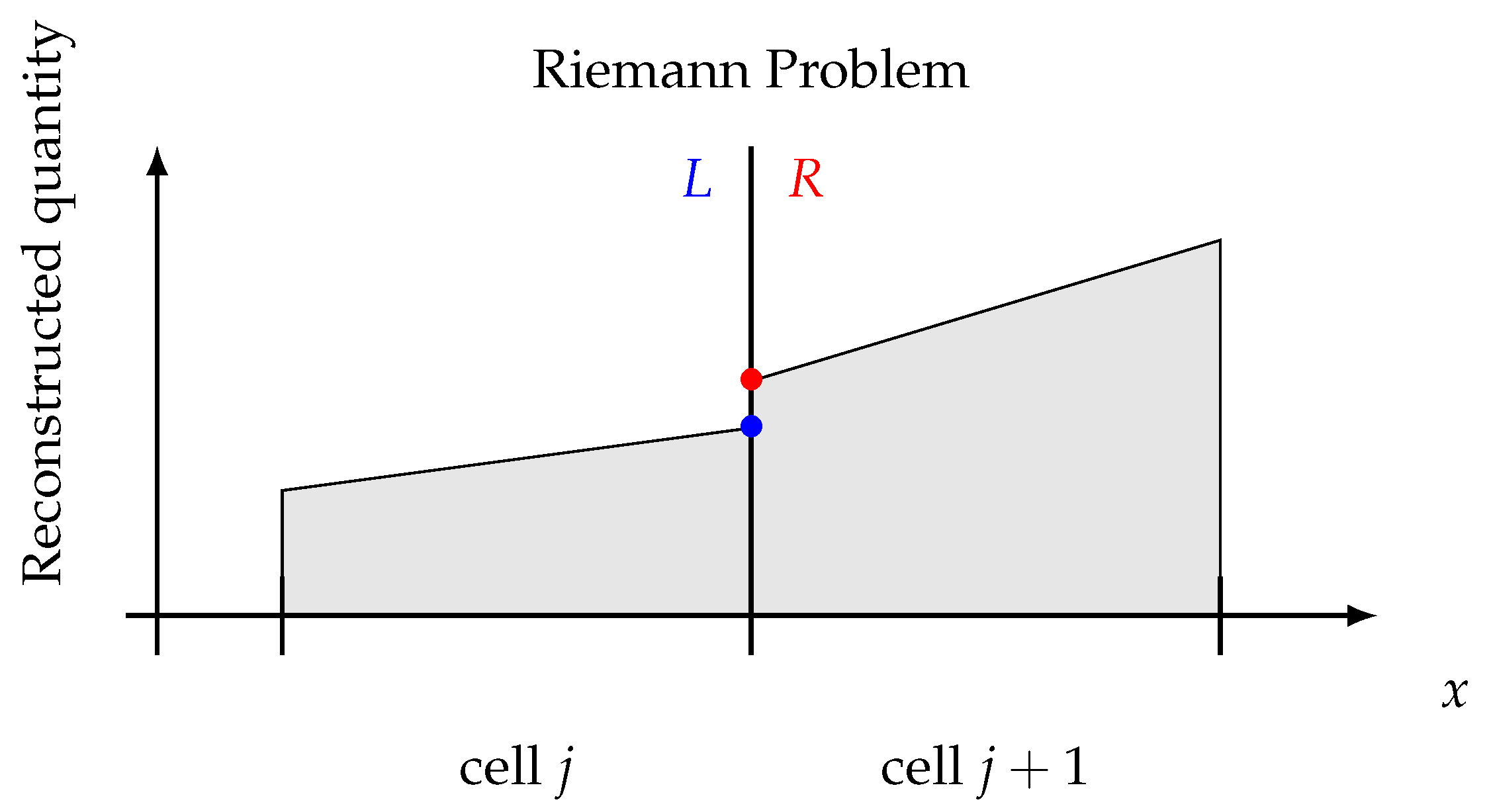
Even by reconstructing the flow field piece-wise linearly (or higher order), it yields to discontinuities at the intercells, as shown in Figure 1, i.e., to a Riemann Problem (RP). RPs can be solved in many different ways [17], provided that the solution is consistent with the adopted system of equations, even if approximated.

The Roe Solvers family [18,19,20] expresses the interface solution as the following:

$$U^{\mathrm{if}}={\displaystyle \frac{U_R+U_L}{2}}-\frac{1}{2}\tilde{\mathbf{R}}\frac{|\tilde{\mathrm{\Lambda }}|}{\tilde{\mathrm{\Lambda }}}\tilde{\mathbf{L}}\left(U_R-U_L\right)$$

(17a)

$$F^{\mathrm{if}}={\displaystyle \frac{F_R+F_L}{2}}-\frac{1}{2}\tilde{\mathbf{R}}\left|\tilde{\mathrm{\Lambda }}\right|\tilde{\mathbf{L}}\left(U_R-U_L\right)$$

(17b)

where $\tilde{\mathrm{\Lambda }}$, $\tilde{\mathbf{L}}$ and $\tilde{\mathbf{R}}$ are the Jacobian eigenvalues and left and right eigenvectors matrices, respectively, and U and F are state and flux vectors, as in Equation (10). Superscript “if” stands for interface, while L and R stand for left and right sides of the interface, as shown in Figure 1. Tilded variables are computed at one specific average state, called the Roe state, researched here, around which the solution is linearized. It is worth to notice that Equation (17)—with no tildes—is always valid for any state, given that left and right states are close to each other. If they are not, the Roe state has to be constructed in such a way that jump relations are satisfied. Lastly, the original hyperbolicity of the system of equations has to be preserved as follows [17,18,19,20].

Summarizing, we have the following:

$$\{\begin{array}{c}\mathrm{Hyperbolicity}\Rightarrow \mathrm{Real}\mathrm{eigenvalues}\hfill \\ \mathrm{Consistency}\Rightarrow \tilde{\mathbf{J}}\mathrm{such}\mathrm{that}\tilde{\mathbf{J}}(U,U)=\mathbf{J}\left(U\right)\hfill \\ \mathrm{Jump}\mathrm{relations}\Rightarrow F_L-F_R=\tilde{\mathbf{J}}(U_L-U_R)\hfill \end{array}$$

(18)

Since cross-section area variations can be treated as source terms, as can be seen in Equations (10) and (11), the Riemann solver can be derived from the homogeneous 5-by-5 system of equations.

Following developments in [17,20] while selecting a different set of primitive variables W as

$$W:={\{\rho ,u,T,Y_o,Y_f\}}^T$$

(19)

a change of coordinates causes the homogeneous system (10) to become the following:

$$\begin{array}{l}\frac{\partial U}{\partial W}\frac{\partial W}{\partial t}+\frac{\partial F}{\partial U}\frac{\partial U}{\partial W}\frac{\partial W}{\partial x}=0\Rightarrow \\ \frac{\partial W}{\partial t}+{\left(\frac{\partial U}{\partial W}\right)}^{-1}\frac{\partial F}{\partial U}\frac{\partial U}{\partial W}\frac{\partial W}{\partial x}=0\Rightarrow \\ \frac{\partial W}{\partial t}+{\left(\frac{\partial U}{\partial W}\right)}^{-1}\frac{\partial F}{\partial W}\frac{\partial W}{\partial x}=0\end{array}$$

(20)

thus, a new Jacobian matrix $\mathbf{K}$ is obtained, in the new set of coordinates W, as the following:

$$\mathbf{K}:={\left(\frac{\partial U}{\partial W}\right)}^{-1}\frac{\partial F}{\partial W}$$

(21)

By developing computations, and using the compact notation for derivatives (${\varphi }_{\psi }:=\partial \varphi /\partial \psi$), matrices become the following:

$$\frac{\partial U}{\partial W}=\left(\begin{array}{ccccc}1& 0& 0& 0& 0\\ \\ u& \rho & 0& 0& 0\\ \\ \rho e_{\rho }+e+{\displaystyle \frac{u^2}{2}}& \rho u& \rho e_T& \rho e_{Y_o}& \rho e_{Y_f}\\ \\ Y_o& 0& 0& \rho & 0\\ \\ Y_f& 0& 0& 0& \rho \\ \end{array}\right)$$

(22)

$$\frac{\partial F}{\partial W}=\left(\begin{array}{ccccc}u& \rho & 0& 0& 0\\ \\ p_{\rho }+u^2& 2\rho u& p_T& p_{Y_o}& p_{Y_f}\\ \\ u\left(\rho e_{\rho }+e+p_{\rho }+{\displaystyle \frac{u^2}{2}}\right)& e\rho +p+{\displaystyle \frac{3\rho u^2}{2}}& u\left(\rho e_T+p_T\right)& u\left(\rho e_{Y_o}+p_{Y_o}\right)& u\left(\rho e_{Y_f}+p_{Y_f}\right)\\ \\ u{Y}_o& \rho Y_o& 0& \rho u& 0\\ \\ u{Y}_f& \rho Y_f& 0& 0& \rho u\\ \end{array}\right)$$

(23)

and thus, the Jacobian $\mathbf{K}$ reads as the following:

$$\mathbf{K}=\left(\begin{array}{ccccc}u& \rho & 0& 0& 0\\ \\ {\displaystyle \frac{p_{\rho }}{\rho }}& u& {\displaystyle \frac{p_T}{\rho }}& {\displaystyle \frac{p_{Y_o}}{\rho }}& {\displaystyle \frac{p_{Y_f}}{\rho }}\\ \\ 0& {\displaystyle \frac{p-{\rho }^2{e}_{\rho }}{\rho e_T}}& u& 0& 0\\ \\ 0& 0& 0& u& 0\\ \\ 0& 0& 0& 0& u\end{array}\right)$$

(24)

Computing eigenvalues yields the following:

$$\mathrm{diag}\left(\mathrm{\Lambda }\right)=\left\{u,u,u,u-a,u+a\right\},\mathrm{where}{a}^2:={\displaystyle \frac{1}{e_T}}\left({\displaystyle \frac{p{p}_T}{{\rho }^2}}-e_{\rho }{p}_T\right)+p_{\rho }=\frac{c_p}{c_v}{p}_{\rho }$$

(25)

while right and left eigenvectors, listed in matrices ${\mathbf{R}}_{\mathbf{K}}$ and ${\mathbf{L}}_{\mathbf{K}}$ by columns and rows, respectively, read as follows:

$${\mathbf{R}}_{\mathbf{K}}=\left(\begin{array}{ccccc}-{\displaystyle \frac{p_{Y_f}}{p_{\rho }}}& -{\displaystyle \frac{p_{Y_o}}{p_{\rho }}}& -{\displaystyle \frac{p_T}{p_{\rho }}}& {\displaystyle \frac{{\rho }^2{e}_T}{p-{\rho }^2{e}_{\rho }}}& {\displaystyle \frac{{\rho }^2{e}_T}{p-{\rho }^2{e}_{\rho }}}\\ \\ 0& 0& 0& {\displaystyle \frac{a\rho e_T}{{\rho }^2{e}_{\rho }-p}}& {\displaystyle \frac{a\rho e_T}{p-{\rho }^2{e}_{\rho }}}\\ \\ 0& 0& 1& 1& 1\\ \\ 0& 1& 0& 0& 0\\ \\ 1& 0& 0& 0& 0\end{array}\right)$$

(26)

$${\mathbf{L}}_{\mathbf{K}}=\left(\begin{array}{ccccc}0& 0& 0& 0& 1\\ \\ 0& 0& 0& 1& 0\\ \\ {\displaystyle \frac{p_{\rho }\left(p_{\rho }-a^2\right)}{a^2{p}_T}}& 0& {\displaystyle \frac{p_{\rho }}{a^2}}& {\displaystyle \frac{p_{Y_o}\left(p_{\rho }-a^2\right)}{a^2{p}_T}}& {\displaystyle \frac{p_{Y_f}\left(p_{\rho }-a^2\right)}{a^2{p}_T}}\\ \\ {\displaystyle \frac{p_{\rho }\left(a^2-p_{\rho }\right)}{2a^2{p}_T}}& {\displaystyle \frac{\rho \left(p_{\rho }-a^2\right)}{2a{p}_T}}& {\displaystyle \frac{1}{2}}-{\displaystyle \frac{p_{\rho }}{2a^2}}& {\displaystyle \frac{p_{Y_o}\left(a^2-p_{\rho }\right)}{2a^2{p}_T}}& {\displaystyle \frac{p_{Y_f}\left(a^2-p_{\rho }\right)}{2a^2{p}_T}}\\ \\ {\displaystyle \frac{p_{\rho }\left(a^2-p_{\rho }\right)}{2a^2{p}_T}}& {\displaystyle \frac{\rho \left(a^2-p_{\rho }\right)}{2a{p}_T}}& {\displaystyle \frac{1}{2}}-{\displaystyle \frac{p_{\rho }}{2a^2}}& {\displaystyle \frac{p_{Y_o}\left(a^2-p_{\rho }\right)}{2a^2{p}_T}}& {\displaystyle \frac{p_{Y_f}\left(a^2-p_{\rho }\right)}{2a^2{p}_T}}\\ \end{array}\right)$$

(27)

For convenience, it is possible to recast the last condition in Equation (18) as the following:

$$\{\begin{array}{c}\Delta U=\tilde{\mathbf{H}}\Delta W\hfill \\ \Delta F=\tilde{\mathbf{A}}\Delta W\hfill \end{array}$$

(28)

where

$$\Delta W={\{\Delta \rho ,\Delta u,\Delta T,\Delta Y_o,\Delta Y_f\}}^T$$

(29a)

$$\Delta U={\{\Delta \rho ,\Delta \left(\rho u\right),\Delta \left(\rho e_0\right),\Delta \left(\rho Y_o\right),\Delta \left(\rho Y_f\right)\}}^T$$

(29b)

$$\Delta F={\{\Delta \left(\rho u\right),\Delta \left(\rho u^2+p\right),\Delta \left(\rho u{h}_0\right),\Delta \left(\rho u{Y}_o\right),\Delta \left(\rho u{Y}_f\right)\}}^T$$

(29c)

and where symbol $\Delta$ represents left-to-right quantity differences ($\Delta \varphi :={\varphi }_L-{\varphi }_R$), and where matrices $\tilde{\mathbf{H}}$, $\tilde{\mathbf{A}}$, $\widetilde{{\mathbf{L}}_{\mathbf{K}}}$ and $\widetilde{{\mathbf{R}}_{\mathbf{K}}}$ are assumed to have the form of their untilded counterparts, in order to assure hyperbolicity. $\tilde{\mathbf{H}}$ and $\tilde{\mathbf{A}}$ read as the following:

$$\tilde{\mathbf{H}}:=\widetilde{\left({\displaystyle \frac{\partial U}{\partial W}}\right)}=\left(\begin{array}{ccccc}1& 0& 0& 0& 0\\ \\ \tilde{u}& \tilde{\rho }& 0& 0& 0\\ \\ \tilde{\rho }{\tilde{e}}_{\rho }+\tilde{e}+{\displaystyle \frac{{\tilde{u}}^2}{2}}& \tilde{\rho }\tilde{u}& \tilde{\rho }{\tilde{e}}_T& \tilde{\rho }{\tilde{e}}_{Y_o}& \tilde{\rho }{\tilde{e}}_{Y_f}\\ \\ {\tilde{Y}}_o& 0& 0& \tilde{\rho }& 0\\ \\ {\tilde{Y}}_f& 0& 0& 0& \tilde{\rho }\\ \end{array}\right)$$

(30)

$$\tilde{\mathbf{A}}:=\widetilde{\left({\displaystyle \frac{\partial F}{\partial W}}\right)}=\left(\begin{array}{ccccc}\tilde{u}& \tilde{\rho }& 0& 0& 0\\ \\ {\tilde{p}}_{\rho }+{\tilde{u}}^2& 2\tilde{\rho }\tilde{u}& {\tilde{p}}_T& {\tilde{p}}_{Y_o}& {\tilde{p}}_{Y_f}\\ \\ \tilde{u}\left(\tilde{\rho }{\tilde{e}}_{\rho }+\tilde{e}+{\tilde{p}}_{\rho }\right)+{\displaystyle \frac{{\tilde{u}}^3}{2}}& \tilde{e}\tilde{\rho }+\tilde{p}+{\displaystyle \frac{3\tilde{\rho }{\tilde{u}}^2}{2}}& \tilde{u}\left(\tilde{\rho }{\tilde{e}}_T+{\tilde{p}}_T\right)& \tilde{u}\left(\tilde{\rho }{\tilde{e}}_{Y_o}+{\tilde{p}}_{Y_o}\right)& \tilde{u}\left(\tilde{\rho }{\tilde{e}}_{Y_f}+{\tilde{p}}_{Y_f}\right)\\ \\ \tilde{u}{\tilde{Y}}_o& \tilde{\rho }{\tilde{Y}}_o& 0& \tilde{\rho }\tilde{u}& 0\\ \\ \tilde{u}{\tilde{Y}}_f& \tilde{\rho }{\tilde{Y}}_f& 0& 0& \tilde{\rho }\tilde{u}\\ \end{array}\right)$$

(31)

Matrix $\tilde{\mathbf{H}}$ is the change-of-coordinates matrix between U and W; thus, the following holds:

$$\tilde{\mathbf{L}}=\widetilde{{\mathbf{L}}_{\mathbf{K}}}{\tilde{\mathbf{H}}}^{-1}$$

(32a)

$$\tilde{\mathbf{R}}=\tilde{\mathbf{H}}\widetilde{{\mathbf{R}}_{\mathbf{K}}}$$

(32b)

Solving system (28) for a consistent (in the sense of Equation (18)) set of averaged variables leads to the Roe state.

Gathering all the unknowns of system (28), considering also Equation (25), results in fourteen unknowns, namely the following:

$$\tilde{\mathrm{Y}}={\tilde{\rho },\tilde{u},\tilde{p},{\tilde{Y}}_o,{\tilde{Y}}_f,\tilde{e},{\tilde{p}}_{\rho },{\tilde{p}}_T,{\tilde{p}}_{Y_o},{\tilde{p}}_{Y_f},{\tilde{e}}_{\rho },{\tilde{e}}_T,{\tilde{e}}_{Y_o},{\tilde{e}}_{Y_f}}^T$$

(33)

while system (28) employs ten equations. They read as follows:

$$\Delta \rho =\Delta \rho$$

(34a)

$$\Delta \left(\rho u\right)=\Delta u\tilde{\rho }+\Delta \rho \tilde{u}$$

(34b)

$$\Delta \left(\rho e_0\right)=\Delta T\tilde{\rho }{\tilde{e}}_T+\Delta \rho \left(\tilde{\rho }{\tilde{e}}_{\rho }+\tilde{e}+\frac{{\tilde{u}}^2}{2}\right)+\Delta Y_f\tilde{\rho }{\tilde{e}}_{Y_f}+\Delta Y_o\tilde{\rho }{\tilde{e}}_{Y_o}+\Delta u\tilde{\rho }\tilde{u}$$

(34c)

$$\Delta \left(\rho Y_o\right)=\Delta Y_o\tilde{\rho }+\Delta \rho {\tilde{Y}}_o$$

(34d)

$$\Delta \left(\rho Y_f\right)=\Delta Y_f\tilde{\rho }+\Delta \rho {\tilde{Y}}_f$$

(34e)

$$\Delta \left(\rho u\right)=\Delta u\tilde{\rho }+\Delta \rho \tilde{u}$$

(34f)

$$\Delta \left(\rho u^2+p\right)=\Delta T{\tilde{p}}_T+\Delta \rho \left({\tilde{p}}_{\rho }+{\tilde{u}}^2\right)+\Delta Y_f{\tilde{p}}_{Y_f}+\Delta Y_o{\tilde{p}}_{Y_o}+2\Delta u\tilde{\rho }\tilde{u}$$

(34g)

$$\begin{array}{c}\Delta \left(\rho u{h}_0\right)=\Delta T\tilde{u}\left(\tilde{\rho }{\tilde{e}}_T+{\tilde{p}}_T\right)+\Delta \rho \left(\tilde{u}\left(\tilde{\rho }{\tilde{e}}_{\rho }+\tilde{e}+{\tilde{p}}_{\rho }\right)+\frac{{\tilde{u}}^3}{2}\right)+\hfill \\ \hfill \hspace{1em}\hspace{1em}\hspace{1em}\hspace{1em}\hspace{1em}\hspace{1em}+\Delta u\left(\tilde{e}\tilde{\rho }+\tilde{p}+\frac{3\tilde{\rho }{\tilde{u}}^2}{2}\right)+\Delta Y_f\tilde{u}\left(\tilde{\rho }{\tilde{e}}_{Y_f}+{\tilde{p}}_{Y_f}\right)+\Delta Y_o\tilde{u}\left(\tilde{\rho }{\tilde{e}}_{Y_o}+{\tilde{p}}_{Y_o}\right)\end{array}$$

(34h)

$$\Delta \left(\rho u{Y}_o\right)=\Delta Y_o\tilde{\rho }\tilde{u}+\Delta \rho \tilde{u}{\tilde{Y}}_o+\Delta u\tilde{\rho }{\tilde{Y}}_o$$

(34i)

$$\Delta \left(\rho u{Y}_f\right)=\Delta Y_f\tilde{\rho }\tilde{u}+\Delta \rho \tilde{u}{\tilde{Y}}_f+\Delta u\tilde{\rho }{\tilde{Y}}_f$$

(34j)

It is worth to notice that there are more unknowns than equations in the problem. Moreover, Equation (34a) is automatically satisfied, while Equation (34b,f), is redundant. Furthermore, as anticipated, the eight pressure and energy partial derivatives appear only in (34c,g,h). For those reasons, the system is not uniquely determined and some additional modeling is required, as expected [20].

3.2.1. Density and Velocity

Following the original formulation [20], density is consistently assumed to be the following:

$$\tilde{\rho }:=\sqrt{{\rho }_L{\rho }_R}$$

(35)

and keeping in mind that for a finite difference, the following equality holds:

$$\Delta \left(\varphi ·\psi \right)=\overline{\varphi }\Delta \psi +\overline{\psi }\Delta \varphi$$

(36)

where

$$\Delta \psi :={\psi }_L-{\psi }_R$$

(37a)

$$\overline{\psi }:={\displaystyle \frac{{\psi }_L+{\psi }_R}{2}}$$

(37b)

Equation (34f) can be recast as the following:

$${\rho }_L{u}_L+\tilde{\rho }{u}_R+{\rho }_R\tilde{u}={\rho }_R{u}_R+\tilde{\rho }{u}_L+{\rho }_L\tilde{u}$$

(38)

where substituting Equation (35) allows to solve for $\tilde{u}$ as the following:

$$\tilde{u}=\frac{\sqrt{{\rho }_L}{u}_L+\sqrt{{\rho }_R}{u}_R}{\sqrt{{\rho }_L}+\sqrt{{\rho }_R}}$$

(39)

3.2.2. Mass Fractions

Substituting quantities obtained so far into Equation (34d,e) gives the following:

$${\tilde{Y}}_o={\displaystyle \frac{\sqrt{{\rho }_L}{Y}_{o,L}+\sqrt{{\rho }_R}{Y}_{o,R}}{\sqrt{{\rho }_L}+\sqrt{{\rho }_R}}}$$

(40)

$${\tilde{Y}}_f={\displaystyle \frac{\sqrt{{\rho }_L}{Y}_{f,L}+\sqrt{{\rho }_R}{Y}_{f,R}}{\sqrt{{\rho }_L}+\sqrt{{\rho }_R}}}$$

(41)

3.2.3. Total Internal Energy

The total internal energy ($e_0$) can be deduced from Equation (34c), as follows. Being that $e_0$ is the function of

$$e_0:=e_0\left(\rho ,T,Y_o,Y_f,u\right)$$

(42)

its total differential and partial derivatives read as the following:

$$\mathrm{d}{e}_0=\frac{\partial e_0}{\partial \rho }\mathrm{d}\rho +\frac{\partial e_0}{\partial T}\mathrm{d}T+\frac{\partial e_0}{\partial Y_o}\mathrm{d}{Y}_o+\frac{\partial e_0}{\partial Y_f}\mathrm{d}{Y}_f+\frac{\partial e_0}{\partial u}\mathrm{d}u$$

(43a)

$$\frac{\partial e_0}{\partial \rho }=\frac{\partial e}{\partial \rho }$$

(43b)

$$\frac{\partial e_0}{\partial T}=\frac{\partial e}{\partial T}$$

(43c)

$$\frac{\partial e_0}{\partial Y_o}=\frac{\partial e}{\partial Y_o}$$

(43d)

$$\frac{\partial e_0}{\partial Y_f}=\frac{\partial e}{\partial Y_f}$$

(43e)

$$\frac{\partial e_0}{\partial u}=u$$

(43f)

thus, Equation (34c) can be recast as the following:

$$\Delta \rho e_0=\Delta \rho \left(\tilde{e}+\frac{{\tilde{u}}^2}{2}\right)+\tilde{\rho }\left(\Delta \rho {\tilde{e}}_{\rho }+\Delta T{\tilde{e}}_T+\Delta Y_f{\tilde{e}}_{Y_f}+\Delta Y_o{\tilde{e}}_{Y_o}+\Delta u\tilde{u}\right)$$

At this point, a new equation for the Roe’ state is introduced on the basis of energy differential, and it reads as the following:

$$\Delta e_0={\tilde{e}}_{0,\rho }\Delta \rho +{\tilde{e}}_{0,T}\Delta T+{\tilde{e}}_{0,u}\Delta u+{\tilde{e}}_{0,Y_f}\Delta Y_f+{\tilde{e}}_{0,Y_o}\Delta Y_o$$

(44)

Recasting again Equation (34c) using Equation (44) and defining ${\tilde{e}}_0$ as

$${\tilde{e}}_0:=\tilde{e}+{\displaystyle \frac{\tilde{u}}{2}}$$

(45)

gives the following:

$$\Delta e_0\rho +\Delta \rho e_0=\Delta e_0\tilde{\rho }+\Delta \rho {\tilde{e}}_0$$

where solving for ${\tilde{e}}_0$ yields the following:

$${\tilde{e}}_0={\displaystyle \frac{\sqrt{{\rho }_L}{e}_{0,L}+\sqrt{{\rho }_R}{e}_{0,R}}{\sqrt{{\rho }_L}+\sqrt{{\rho }_R}}}$$

(46)

As a consequence, internal energy ($\tilde{e}$) reads as the following:

$$\tilde{e}={\tilde{e}}_0-{\displaystyle \frac{{\tilde{u}}^2}{2}}=\frac{e_L\sqrt{{\rho }_L}+e_R\sqrt{{\rho }_R}}{\sqrt{{\rho }_L}+\sqrt{{\rho }_R}}+\frac{\sqrt{{\rho }_L}\sqrt{{\rho }_R}{(u_L-u_R)}^2}{2{\left(\sqrt{{\rho }_L}+\sqrt{{\rho }_R}\right)}^2}$$

(47)

It is important to remark that such determination of internal energies is not unique. In fact, the usage of the finite difference decomposition, as in Equation (36), allows to solve Equation (34c) also for internal energy ($\tilde{e}$) directly. Such manipulation is possible, provided the inclusion of the counterpart of Equation (44), written for $\Delta \tilde{e}$. It ends up with the internal energy ($\tilde{e}$) having the form of Equation (46), while the total internal energy (${\tilde{e}}_0$) has the form of Equation (47), with opposite signs.

3.3. Enthalpy

Using exactly the same procedure as done for internal energy, it is possible to solve Equation (34h) for total specific enthalpy. The procedure is identical and thus synthesized for brevity. Introducing the definition of tilded, the total specific enthalpy is the following:

$${\tilde{h}}_0:=\tilde{h}+{\displaystyle \frac{{\tilde{u}}^2}{2}}:=\tilde{e}+{\displaystyle \frac{\tilde{p}}{\tilde{\rho }}}+{\displaystyle \frac{{\tilde{u}}^2}{2}}$$

(48)

including the definition of enthalpy discrete differential ($\Delta h_0$), as done for energy,

$$\Delta h_0={\tilde{h}}_{0,\rho }\Delta \rho +{\tilde{h}}_{0,T}\Delta T+{\tilde{h}}_{0,u}\Delta u+{\tilde{h}}_{0,Y_f}\Delta Y_f+{\tilde{h}}_{0,Y_o}\Delta Y_o$$

(49)

and substituting it into Equation (34h) yields the following:

$$\Delta \left(\rho uh0\right)={\tilde{h}}_0(\Delta u\tilde{\rho }+\Delta \rho \tilde{u})+\Delta h_0\tilde{\rho }\tilde{u}$$

(50)

Solving for ${\tilde{h}}_0$ results in the following:

$${\tilde{h}}_0=\frac{h_{0,L}\sqrt{\rho L}+h_{0,R}\sqrt{\rho R}}{\sqrt{\rho L}+\sqrt{\rho R}}$$

(51)

Specific enthalpy can be obtained from Equation (48): the result is analogous to the energy result.

In addition, concerning enthalpy, it is worth to note that Equation (34h) can be solved for total specific enthalpy (${\tilde{h}}_0$), specific enthalpy ($\tilde{h}$), or total enthalpy per unit volume ($\widetilde{\rho h_0}$). Solving for $\widetilde{\rho h_0}$ yields a solution that is coincident with the one just showed ($\widetilde{\rho h_0}\equiv \tilde{\rho }{\tilde{h}}_0$). On the other hand, solving for $\tilde{h}$ results in a completely different expression, that is more complicated and computationally intensive for all the quantities.

For the sake of simplicity and computational speed, Equations (34c,h) are chosen to be solved for ${\tilde{e}}_0$ and ${\tilde{h}}_0$, respectively.

3.4. Pressure

Pressure is defined as the difference between ${\tilde{h}}_0$ and ${\tilde{e}}_0$:

$$\tilde{p}=\tilde{\rho }\left(\widetilde{h_0}-\widetilde{e_0}\right)$$

(52)

yielding the following:

$$\begin{array}{c}{\tilde{h}}_0-{\tilde{e}}_0={\displaystyle \frac{\left({\displaystyle \frac{p_L}{{\rho }_L}}\right)\sqrt{{\rho }_L}+\left({\displaystyle \frac{p_R}{{\rho }_R}}\right)\sqrt{{\rho }_R}}{\sqrt{{\rho }_L}+\sqrt{{\rho }_R}}}={\displaystyle \frac{{\displaystyle \frac{p_L}{\sqrt{{\rho }_L}}}+{\displaystyle \frac{p_R}{\sqrt{{\rho }_R}}}}{\sqrt{{\rho }_L}+\sqrt{{\rho }_R}}}\Rightarrow \hfill \\ \Rightarrow \tilde{p}={\displaystyle \frac{p_L\sqrt{{\rho }_R}+p_R\sqrt{{\rho }_L}}{\sqrt{{\rho }_L}+\sqrt{{\rho }_R}}}\end{array}$$

(53)

3.5. Other Equations

Equations in system (34) are all used, except Equation (34i,j,h). Concerning Equation (34i,j), they are identically satisfied by the quantities obtained so far. Concerning Equation (34g) on the other hand, it can be manipulated to obtain the following:

$$\Delta \left(\rho u^2\right)+\Delta p=\Delta \rho {\tilde{u}}^2+2\Delta u\tilde{\rho }\tilde{u}+\left({\tilde{p}}_{\rho }\Delta \rho +{\tilde{p}}_T\Delta T+{\tilde{p}}_{Y_f}\Delta Y_f+{\tilde{p}}_{Y_o}\Delta Y_o\right)$$

(54)

Such an equation can be identically satisfied, provided the inclusion of a discrete differential in tilde variables also for pressure as follows:

$$\Delta p={\tilde{p}}_{\rho }\Delta \rho +{\tilde{p}}_T\Delta T+{\tilde{p}}_{Y_f}\Delta Y_f+{\tilde{p}}_{Y_o}\Delta Y_o$$

(55)

3.6. Partial Derivatives of Pressure and Internal Energy

There are eight quantities yet to be defined in the unknowns vector in Equation (33) and in system (34): they are pressure and internal energy partial derivatives. Since pressure derivatives appear only in their respective tilde differentials definitions, they need to be modeled.

Pressure partial derivatives are evaluated using the same form of pressure as Equation (53) (using the compact notation $p_{\psi }$ := $\partial p/\partial \psi$) as the following:

$${\tilde{p}}_{\rho }=\tilde{\rho }{\displaystyle \frac{\left({\displaystyle \frac{p_{\rho ,L}}{\sqrt{{\rho }_L}}}+{\displaystyle \frac{p_{\rho ,R}}{\sqrt{{\rho }_R}}}\right)}{\sqrt{{\rho }_L}+\sqrt{{\rho }_R}}}$$

(56a)

$${\tilde{p}}_T=\tilde{\rho }{\displaystyle \frac{\left({\displaystyle \frac{p_{T,L}}{\sqrt{{\rho }_L}}}+{\displaystyle \frac{p_{T,R}}{\sqrt{{\rho }_R}}}\right)}{\sqrt{{\rho }_L}+\sqrt{{\rho }_R}}}$$

(56b)

$${\tilde{p}}_{Y_o}=\tilde{\rho }{\displaystyle \frac{\left({\displaystyle \frac{p_{Y_o,L}}{\sqrt{{\rho }_L}}}+{\displaystyle \frac{p_{Y_o,R}}{\sqrt{{\rho }_R}}}\right)}{\sqrt{{\rho }_L}+\sqrt{{\rho }_R}}}$$

(56c)

$$\{\begin{array}{cc}{\tilde{p}}_{Y_f}={\displaystyle \frac{\Delta p-{\tilde{p}}_{\rho }\Delta \rho +{\tilde{p}}_T\Delta T-{\tilde{p}}_u\Delta u-{\tilde{p}}_{Y_o}\Delta Y_o}{\Delta Y_f}}\hfill & \mathrm{if}{Y}_{f,L}\ne Y_{f,R}\\ {\tilde{p}}_{Y_f}=\tilde{\rho }{\displaystyle \frac{\left({\displaystyle \frac{p_{Y_f,L}}{\sqrt{{\rho }_L}}}+{\displaystyle \frac{p_{Y_f,R}}{\sqrt{{\rho }_R}}}\right)}{\sqrt{{\rho }_L}+\sqrt{{\rho }_R}}}\hfill & \hspace{1em}\hspace{1em}\mathrm{if}{Y}_{f,L}=Y_{f,R}=Y_f\end{array}$$

(56d)

where the first case of Equation (56d) is necessary to satisfy Equation (55).

In the same way, energy partial derivatives are taken like the energy definition, Equation (47). They read as the following:

$${\tilde{e}}_{\rho }={\displaystyle \frac{\sqrt{{\rho }_L}{e}_{\rho ,L}+\sqrt{{\rho }_R}{e}_{\rho ,R}}{\sqrt{{\rho }_L}+\sqrt{{\rho }_R}}}+\langle u\rangle$$

(57a)

$${\tilde{e}}_T={\displaystyle \frac{\sqrt{{\rho }_L}{e}_{T,L}+\sqrt{{\rho }_R}{e}_{T,R}}{\sqrt{{\rho }_L}+\sqrt{{\rho }_R}}}+\langle u\rangle$$

(57b)

$${\tilde{e}}_{Y_o}={\displaystyle \frac{\sqrt{{\rho }_L}{e}_{Y_o,L}+\sqrt{{\rho }_R}{e}_{Y_o,R}}{\sqrt{{\rho }_L}+\sqrt{{\rho }_R}}}+\langle u\rangle$$

(57c)

$$\{\begin{array}{cc}{\tilde{e}}_{Y_f}={\displaystyle \frac{\Delta e_0-{\tilde{e}}_{0,\rho }\Delta \rho -{\tilde{e}}_{0,T}\Delta T-{\tilde{e}}_{0,u}\Delta u-{\tilde{e}}_{0,Y_o}\Delta Y_o}{{\tilde{e}}_0\tilde{e}\Delta Y_f}}\hfill & \mathrm{if}{Y}_{f,L}\ne Y_{f,R}\\ {\tilde{e}}_{Y_f}={\displaystyle \frac{\sqrt{{\rho }_L}{e}_{Y_f,L}+\sqrt{{\rho }_R}{e}_{Y_f,R}}{\sqrt{{\rho }_L}+\sqrt{{\rho }_R}}}+\langle u\rangle \hfill & \hspace{1em}\hspace{1em}\mathrm{if}{Y}_{f,L}=Y_{f,R}=Y_f\end{array}$$

(57d)

where $\partial {\tilde{e}}_0/\partial \tilde{e}$ = 1, where

$$\langle u\rangle :=\frac{\sqrt{{\rho }_L}\sqrt{{\rho }_R}{(u_L-u_R)}^2}{2{\left(\sqrt{{\rho }_L}+\sqrt{{\rho }_R}\right)}^2}$$

(58)

and, again, where the first case of Equation (57d) is necessary to satisfy Equation (44).

4. Verification and Validation

The two models developed so far, i.e., the simplified cubic EoS for mixtures and the three-species Roe solver for generic gases, were implemented into an in-house one-dimensional CFD solver. Such a solver employs finite volume first- and second-order Godunov-like numerical schemes.

The verification and validation processes follow different subsequent steps, which was also reported in [22]. First of all, the EoS subroutine is validated against the NIST database, by means of the refprop software [23], for both pure fluids and mixtures. Secondly, RS is validated against ideal gas Riemann problems. It has to be remarked that such a formulation of the Riemann solver is independent of any EoS. For such a reason, the ideal EoS, which was formerly coded in the solver and already validated in previous works (e.g., [24]), it was chosen as a first step of the RS validation. Lastly, the Riemann solver and the EoS are used in synergy to reproduce real gas Riemann problems and simple wave propagation in shock tubes.

Thermodynamic states investigated in this section are those representative of a typical oxidizer post and of a shear coaxial injector mixing zone. The reason for not investigating the hot-gas regime is justified by the fact that combustion products in the chamber core are assumed to behave as an ideal gas mixture as commonly assumed elsewhere [25,26].

4.1. EoS Validation

Validation is performed using each of the three cubic EoS into which Equation (3) can be recast, namely SRK, PR and RK-PR. Density, internal energy and speed of sound are chosen as observables.

4.1.1. Pure Oxygen, Low Temperature

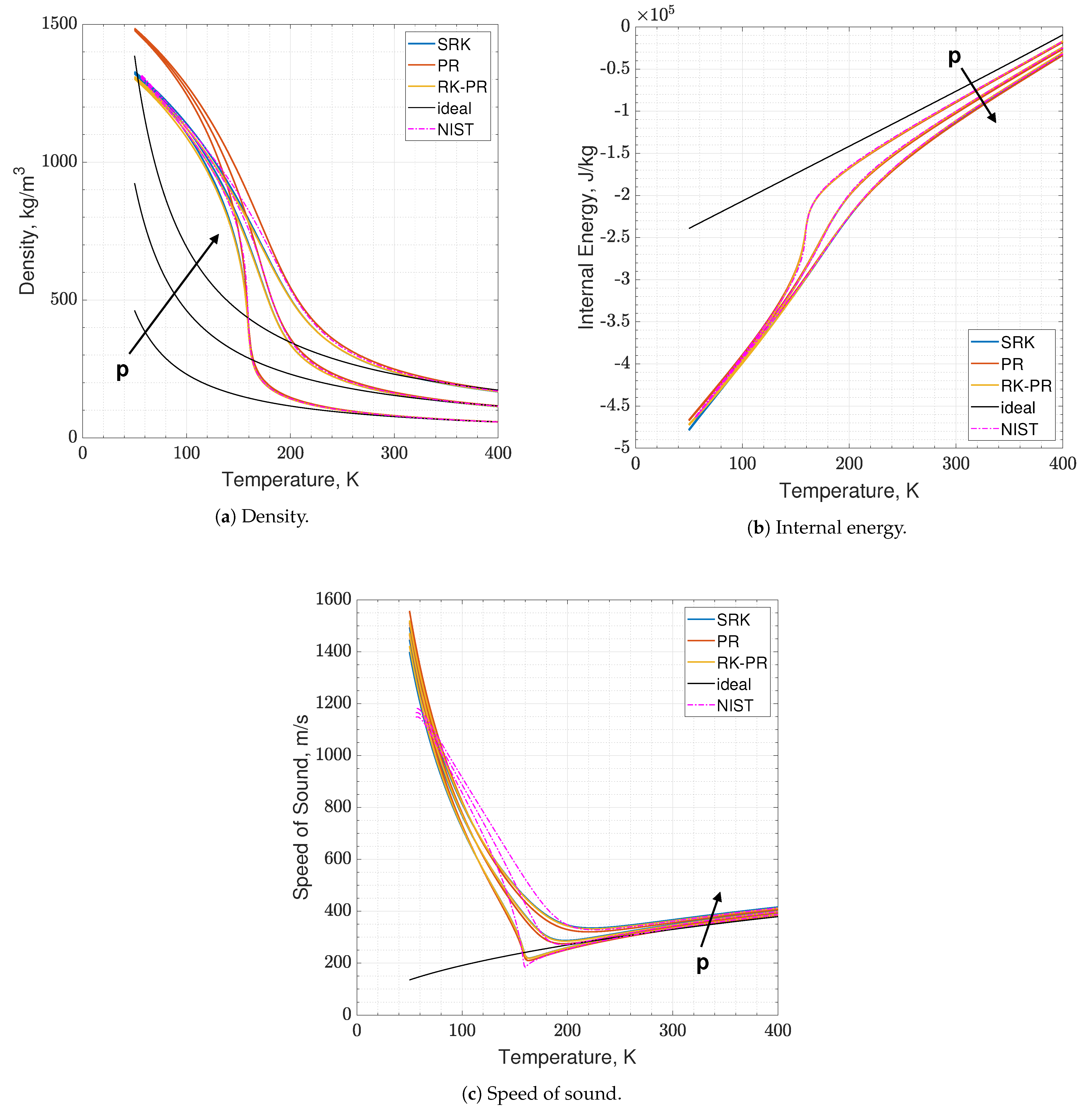
Considering the aforementioned class of problems that will be faced with such a model, it is important to capture the oxidizer’s real fluid behavior. Since the oxidizer comes directly from the tanks or pumps, the investigated temperature range is selected to be 50–400 K, while pressure 6, 12 and 18 MPa. Molecular oxygen ($O_2$) is considered, its properties are listed in

Table 2. Proprieties of molecular oxygen ($O_2$).

Quantity	Symbol	Value	Unit
Critical Temperature	$T_{c,o}$	154.581	K
Critical Pressure	$p_{c,o}$	5.043	MPa
Critical Density	${\rho }_{c,o}$	436.1	kg/m${}^3$
Critical Compressibility	$Z_{c,o}$	0.287925	–
Acentric Factor	${\omega }_o$	0.0222	–
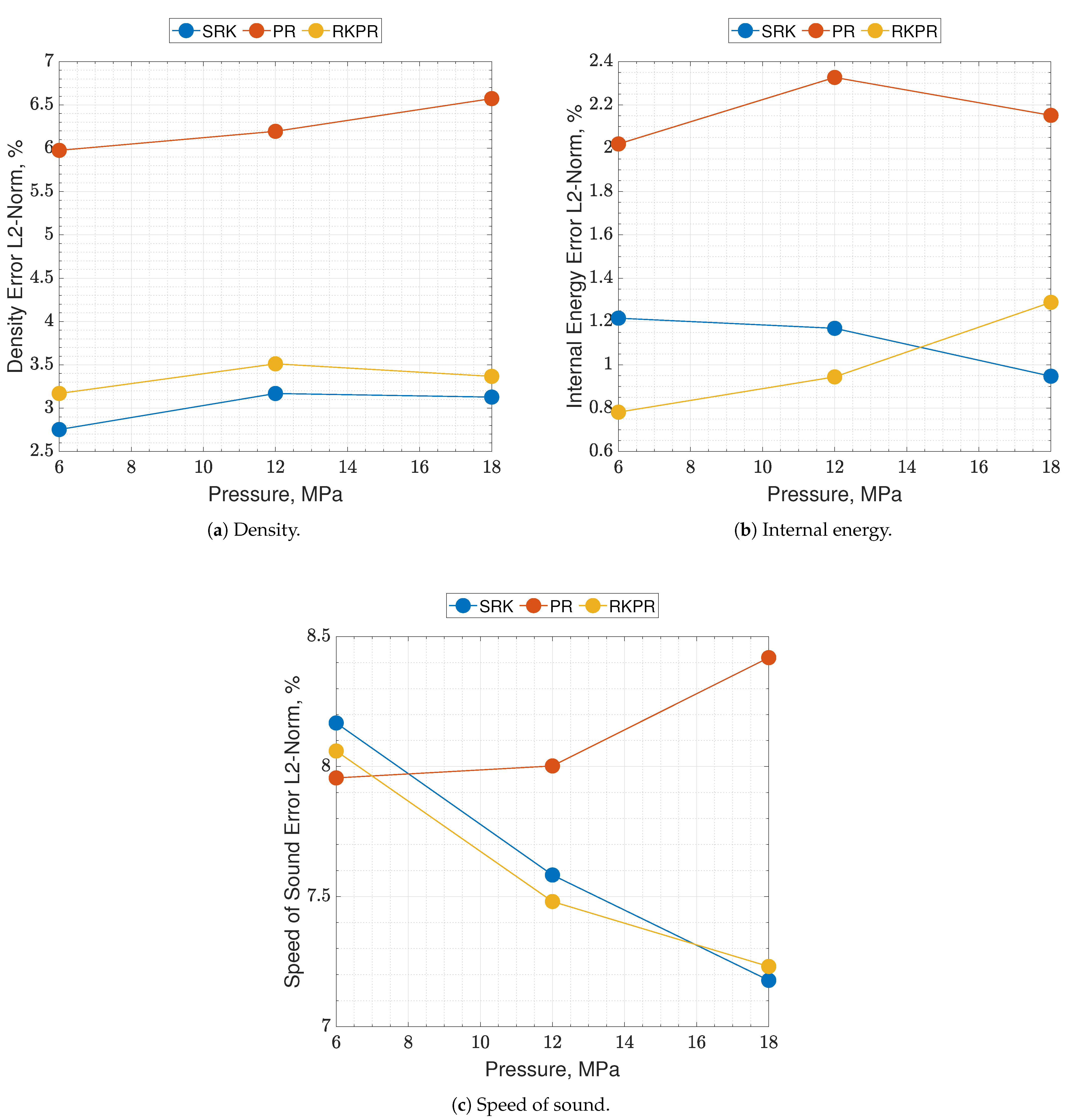
Molecular weight	$w_o$	31.999	kg/kmol

. Errors are estimated as the nondimensionalized L2-norms calculated between the EoS results and the NIST dataset, over the whole temperature range, for a single pressure value.

Results of real $O_2$ are reported in Figure 2 and Figure 3, where the following can be noticed. First of all, supercritical oxygen behavior is qualitatively captured by each of the three EoSs. As the temperature turns higher, all the curves collapse onto the ideal ones, correctly. It appears that different quantities are affected by different levels of errors, e.g., PR EoS seems to show higher displacements on density and internal energy, while speed of sound behaves comparably with the other two EoS, especially at low pressures. Speed of sound is the quantity affected by the greater error with respect to NIST data, reaching an L2-norm error value close to 10% (see Figure 3c), and a local error value that is even higher, up to 20–25% depending on the EoS considered. Such an aspect is expected since it is known in the literature [16].

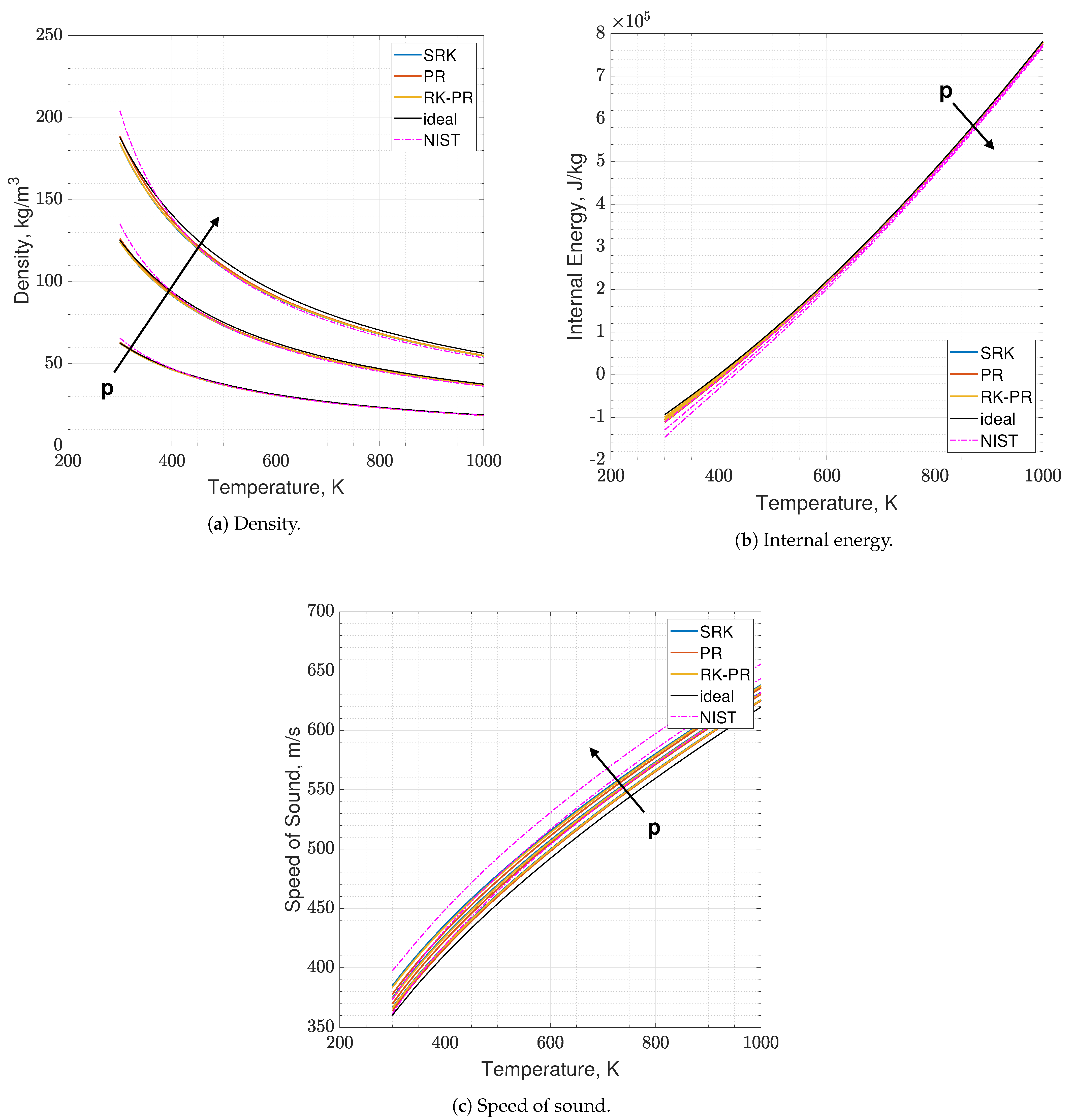
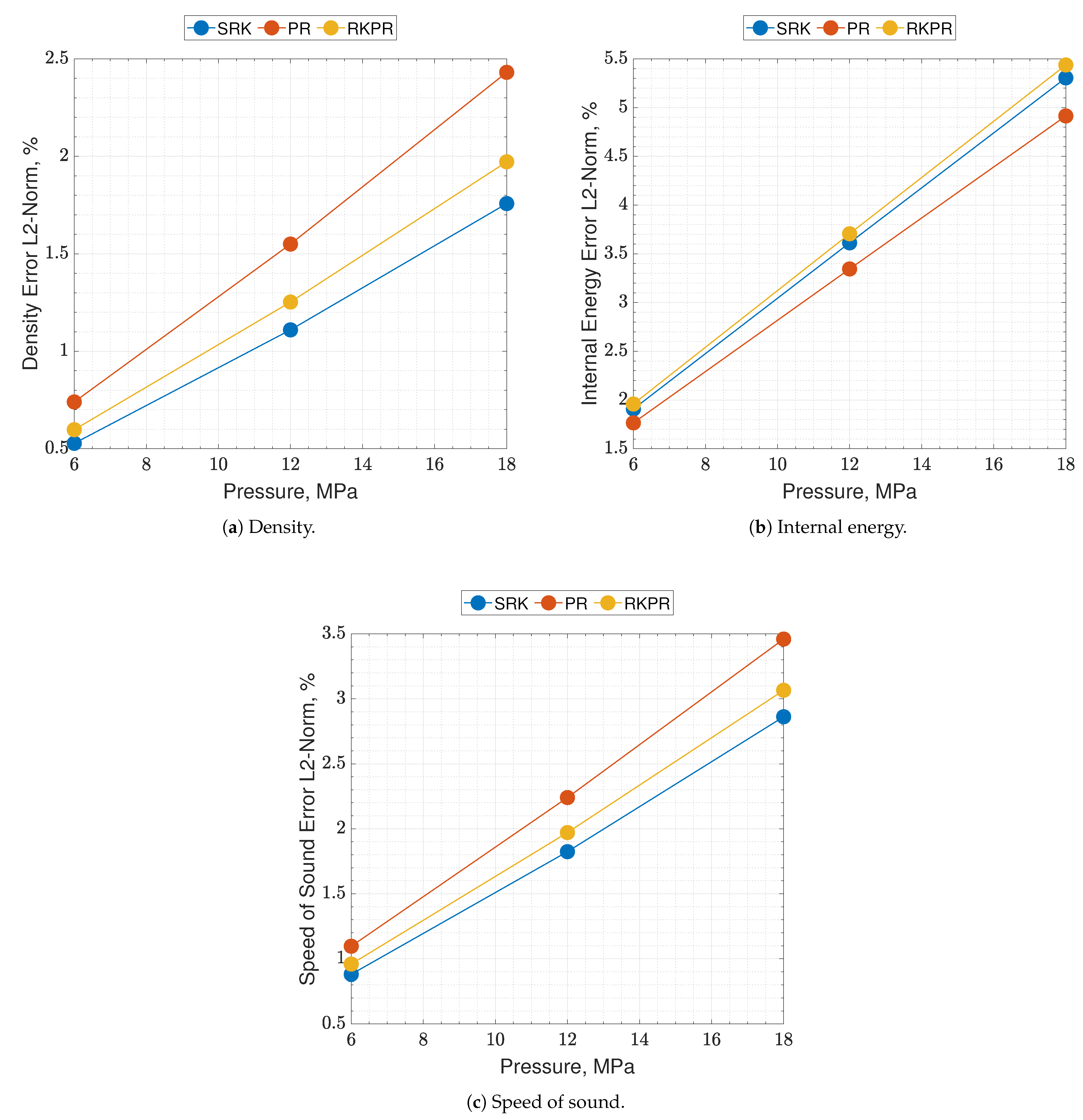
4.1.2. Oxygen–Methane Mixture, Mid Temperature

As a second validation test, the behavior of the EoS dealing with mixtures is assessed. An $O_2$-$C{H}_4$ mixture with an O/F ratio of 3.4 is selected, which is a possible value of interest in liquid rocket engine chambers. It has to be recalled here that methane is treated as an ideal species, while oxygen as a real one. Differently from the oxidizer, fuel comes from the cooling jacket and thus, its temperature might be quite high. For such a reason, the temperature range of 300–1000 K is selected, as it is an interesting range to be investigated. Pressure values are 6, 12 and 18 MPa. Again, errors are estimated as the nondimensionalized L2-norms calculated between the EoS results and the NIST dataset over the whole temperature range for a single pressure value.

The results of the real $O_2$-$C{H}_4$ mixture are available in Figure 4 and Figure 5. It clearly appears in the plots that the real and ideal behaviors are quite close to each other, at those thermodynamic states. The quantity that shows a slightly higher disagreement is again the speed of sound. Concerning the EoSs, they show quite a coincident behavior, in this test. Errors lie between 0.5% and 5.5%, depending on the EoS and on the observable.

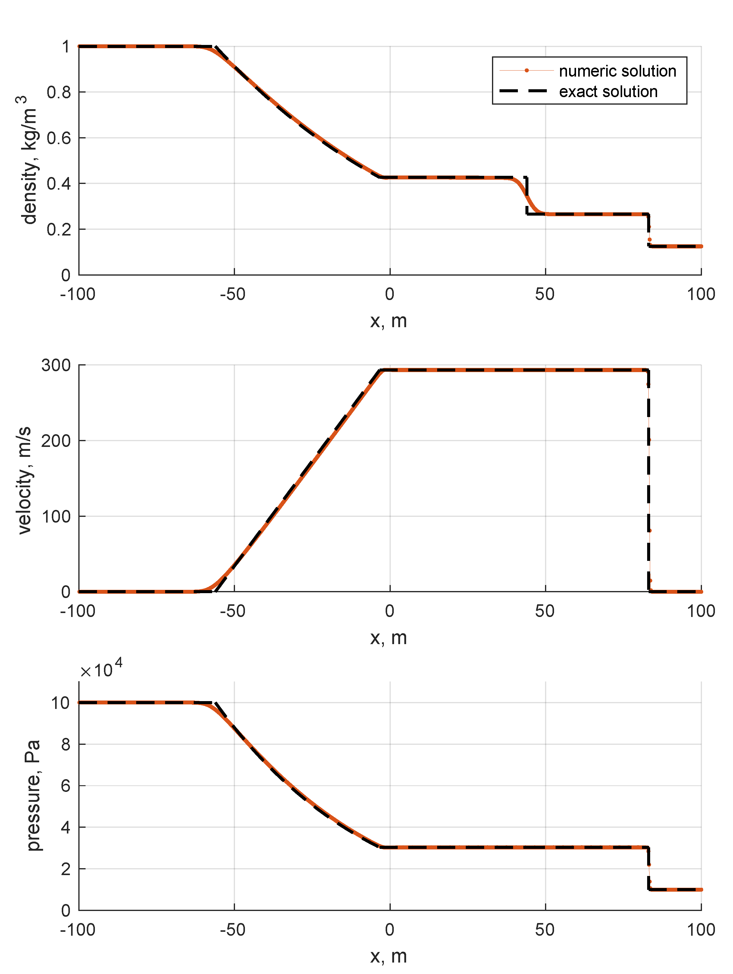
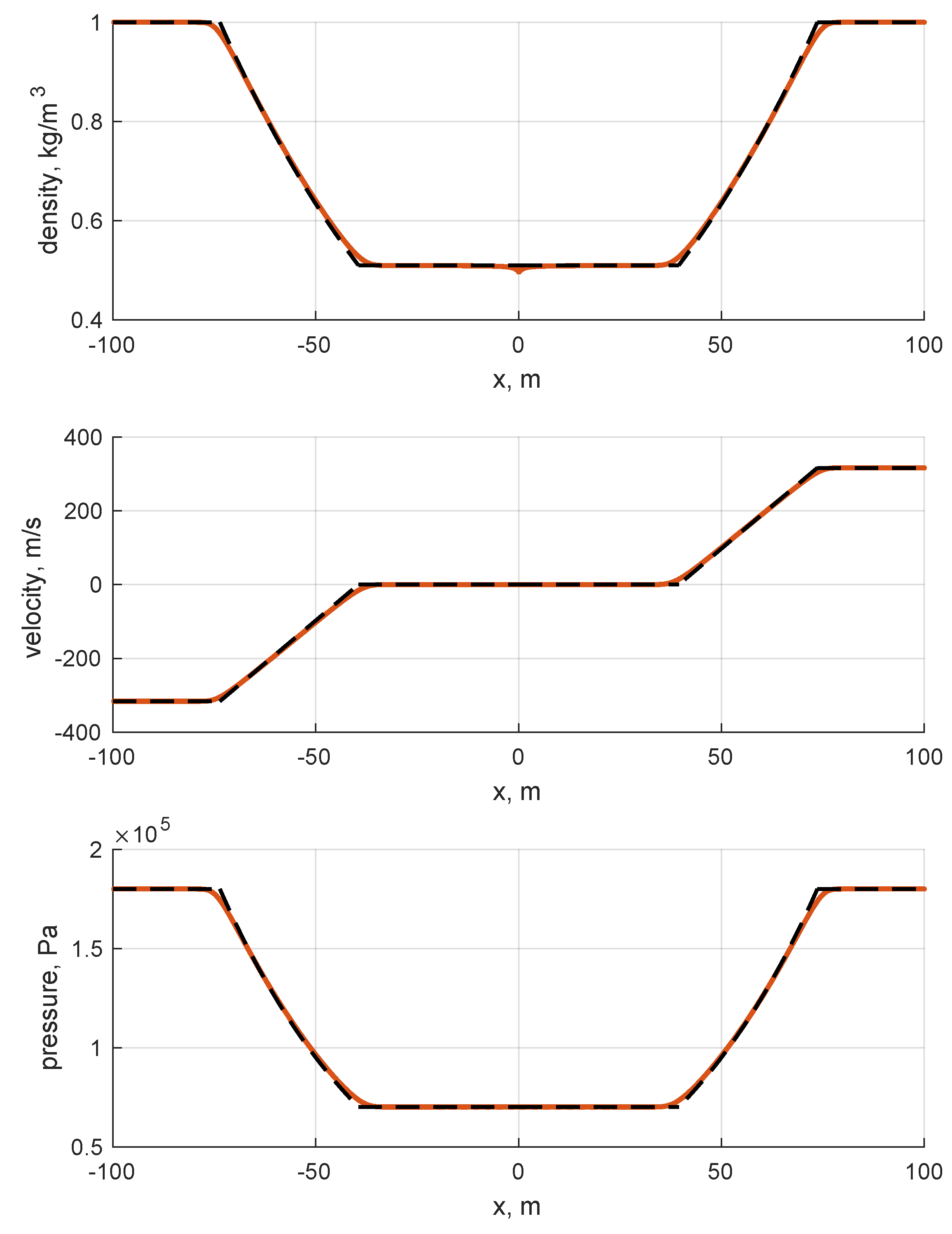
4.1.3. Ideal Gas Riemann Problems

The next step in the validation process involves the Riemann solver. For such a reason, two ideal gas Riemann problems are computed. The reason for such a choice lies in the fact that the ideal EoS was thoroughly validated in previous works (e.g., [24]), and in the fact that the solution of the ideal gas Riemann problems can be easily computed. The solver integrates the full conservative version of conservation laws listed in Equation (10) over a domain discretized in one thousand cells. Even if the number of cells seems high for a plain Riemann problem, it has to be pointed out that the physical length of the domain is 200 m; thus, $\Delta x$ is 20 cm. Such a high space span introduces significant numerical errors. The reason for choosing a domain this wide is justified by the fact that classical non-dimensional Riemann problems do not fit well with gas properties polynomials, so they are treated dimensionally, for convenience. The two selected problems are the Sod problem and the double symmetric expansion problem. The former describes the typical shock tube problem in which the two halves of the domain are separated by a diaphragm and are pressurized differently. In particular, the left-to-right side pressure ratio is 10, while the density ratio is 8. The velocity is uniformly null over the entire domain. As the diaphragm is removed, a rarefaction wave is generated leftwards, which is almost sonic, whilst a contact discontinuity and shock wave begin traveling rightwards (RCS (rarefaction-contact-shock) solution). The latter, the double symmetric expansion problem, considers the two zones as having uniform pressure and density but equal and opposite velocities as the initial condition. In particular, the left-hand side velocity is negative, while the right-hand side value is positive. The anticipated solution is characterized by two expansion waves traveling in both directions symmetrically, with quiescent low pressure fluid in the middle (RNR (rarefaction-null-rarefaction) solution). The initial conditions are summarized in

Table 3. Ideal gas Riemann problems initial conditions.

Problem	Quantity	Value	Units	Type
Sod	$T_L$	348.43	K	enforced
	$T_R$	278.74	K	enforced
	$u_L$	0	m/s	enforced
	$u_R$	0	m/s	enforced
	${\rho }_L$	1	kg/m${}^3$	enforced
	${\rho }_R$	0.125	kg/m${}^3$	enforced
	$p_L$	100	kPa	computed
	$p_R$	10	kPa	computed
Doub. Exp.	$T_L$	627.18	K	enforced
	$T_R$	627.18	K	enforced
	$u_L$	−316.22	m/s	enforced
	$u_R$	316.22	m/s	enforced
	${\rho }_L$	1	kg/m${}^3$	enforced
	${\rho }_R$	1	kg/m${}^3$	enforced
	$p_L$	180	kPa	computed
	$p_R$	180	kPa	computed

.

The results are shown in Figure 6 and Figure 7. By looking at the pictures, the exact solution appears to be well captured. As expected, artificial diffusion appears clearly at the contact discontinuity of the Sod problem and at the expansion front ends in both the Sod and double expansion problems. As expected, a minor numerical issue appears at $x=0$ of the double expansion problem in the density trend. It is motivated by the fact that one eigenvalue is zero there, i.e., the velocity u.

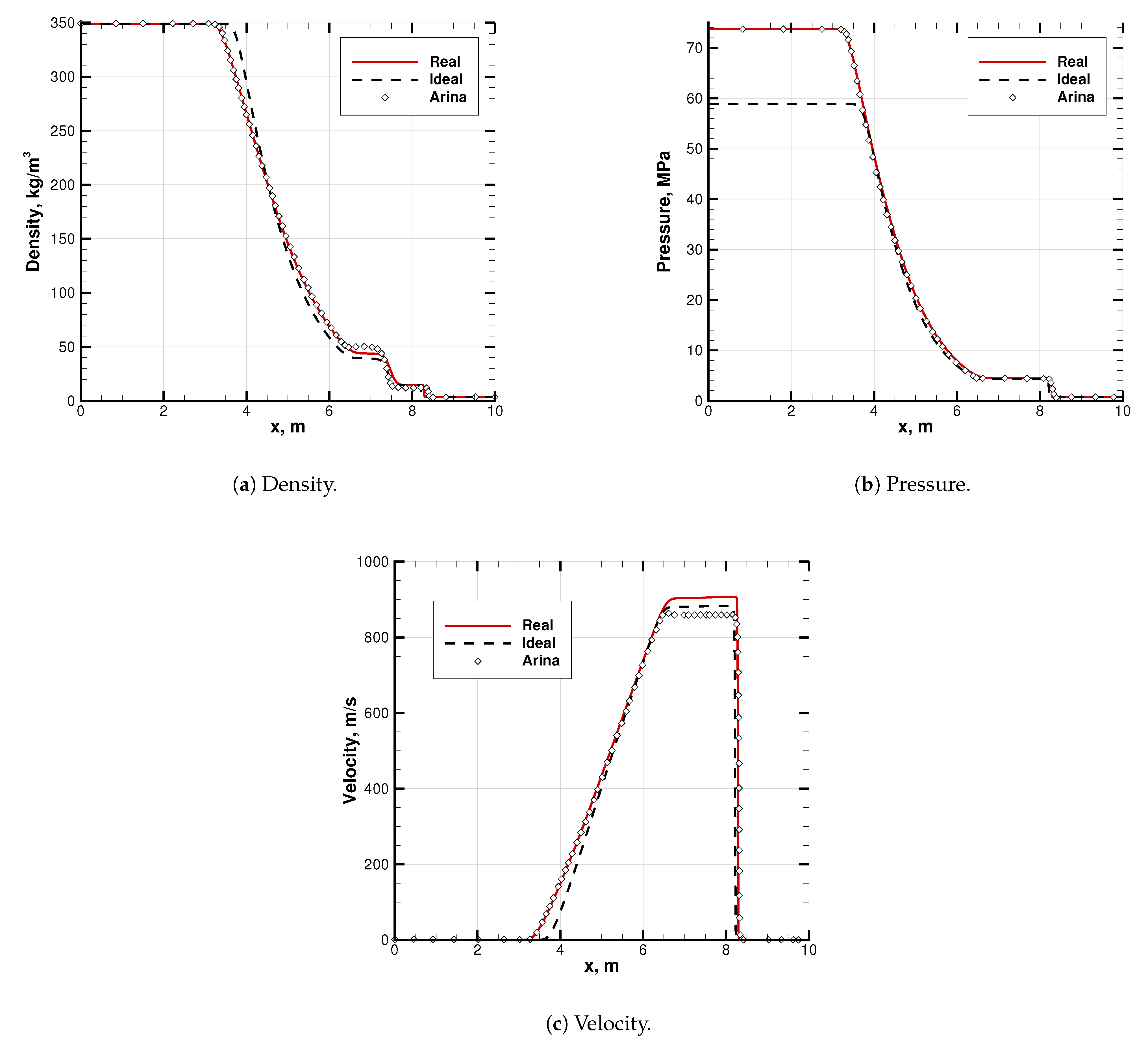
4.1.4. Real Gas Riemann Problems

The next step toward validation is solving a Riemann problem in the real gas regime. Unfortunately, few Riemann problems solutions for real gases are available in the literature. For such a reason, an option to be sought is code-to-code validation, as done, for instance, by Muto et al. [9]. They validated their solutions against that of Arina [27] results. It has to be pointed out that Arina’s solution employs a slightly different EoS, since he uses the plain RK formulation, while here, the EoS is set to use the SRK formulation. The problem is a transonic Sod problem, performed in a real gas regime. Initial conditions are shown in

Table 4. Real gas transonic Sod problem initial conditions.

Quantity	Value	Units	Type
$T_L$	892.67	K	enforced
$T_R$	1116.89	K	enforced
$u_L$	0	m/s	enforced
$u_R$	0	m/s	enforced
${\rho }_L$	348.8	kg/m${}^3$	enforced
${\rho }_R$	3.488	kg/m${}^3$	enforced
$p_L$	73760	kPa	computed
$p_R$	737.6	kPa	computed

.

Results are shown in Figure 8. They agree to a significant extent with Arina’s solution. The slight difference in the EoS is visible in the intermediate states, between the shock and the expansion waves (abscissas $x=[6.5,8.5]$ m), and thus, on the contact discontinuity. Nevertheless, both the waves are well captured (see Figure 8). Note that the real and ideal initial conditions in density and temperature correctly result in different pressures (see Figure 8b).

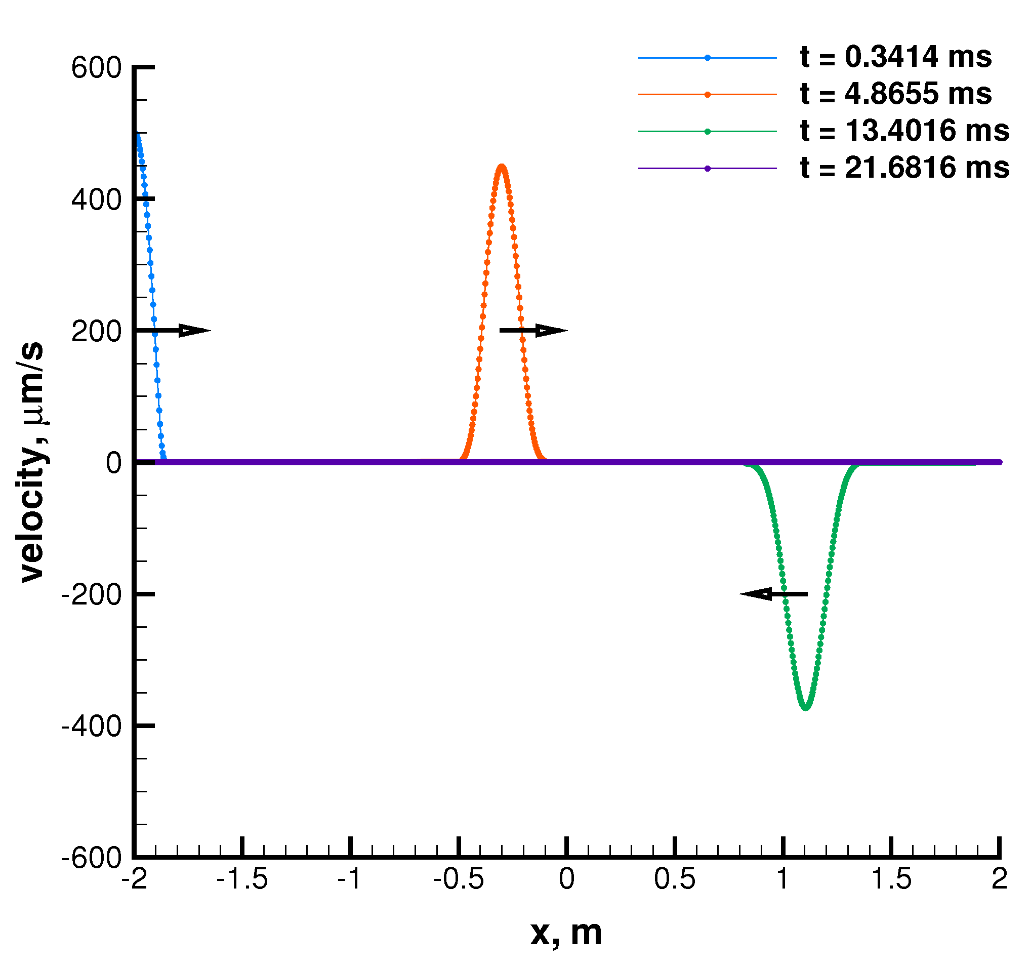
4.1.5. Acoustic Propagation

In order to complete the validation, a test involving mixtures is needed. Unfortunately there are no suitable wave propagation validation cases available in the literature that are close to the present problem, to the knowledge of the authors. For such a reason, a simple propagation test is conceived and simulated, that is, a plain linear disturbance propagation in a quiescent closed-closed tube. A disturbance is enforced on the left boundary, on velocity. The amplitude is small enough to keep the flow field in the linear regime, i.e., small perturbations regime. Its amplitude is selected to be 500 $\mathsf{\mu }$m/s; thus, the velocities of propagation can be approximated to the plain speed of sound. Three tests are carried out employing a real $O_2$-ideal $C{H}_4$ mixture, at O/F = 3.4, at different thermodynamic states representative of actual conditions in the mixing zone of a real engine. Specifically, the pressure is fixed at 12 MPa, while the temperature is selected to be 300, 600 and 1000 K. The speed of sound is estimated as the space traveled by the disturbance divided by the time interval starting from the moment in which its peak enters in the domain, at the left boundary, and ending at the moment in which it is reflected, at the same boundary, after having covered the whole duct back and forth. Such a measure is then compared with refprop values of speed of sound and also with the result provided by the plain EoS in order to assess the error introduced by the RS on such quantity and on propagation dynamics, in general.

Results are shown in Figure 9 for the case with $T=$ 300 K and listed in

Table 5. Duct thermodynamic state during acoustic propagation tests. Mixture is made of $O_2$-$C{H}_4$ with O/F = 3.4.

Domain State	Values			Units	Type
Temperature	300	600	1000	K	enforced
Velocity	0	0	0	m/s	enforced
Density	124.263	60.975	36.862	kg/m${}^3$	enforced
Pressure	12	12	12	MPa	computed
Speed of sound	374.8793	507.3510	631.9814	m/s	numerical propagation
Speed of sound	374.8794	507.3490	631.9807	m/s	present EoS value
Speed of sound	373.4200	516.6100	643.7000	m/s	(refprop)

for all the temperature values. Plots are showed only for the case with $T=$ 300 K since those at $T=$ 600 K and 1000 K only differ from it for the time labels. They show how the speed of sound computed from the results of the propagation test is substantially overlapped onto the value given by the EoS. This means that the RS does not introduce a relevant numerical error which is capable of affecting characteristic times of wave propagation. On the other hand, as expected, propagation tests and plain EoS results differ from refprop to the same extent, due to the error introduced by the cubic formulation. However, the level of agreement can be considered good for those thermodynamic states.

5. Discussion and Conclusions

In this work, a novel thermodynamic modeling approach is derived for dealing with wave propagation in liquid rocket thrust chambers. Such a class of problems is of particular interest for the study of high-frequency combustion instability problems. The adopted approach is selected to be low-order modeling-oriented.

Such modeling consists of the adoption of a cubic equation of state for the mixture, which is then significantly simplified to be a special EoS, describing hybrid real/ideal gas mixtures. The reason for this lies in the fact that in dealing with such a class of problems, the only species which is actually needed to be modeled as a real fluid is the oxidizer. Indeed, considering present cryogenic liquid rocket engines, the oxidizer flows into the injectors and then into the chamber at a significantly low temperature, as it comes directly from either the pump assembly or from its tank. On the other hand, the fuel typically reaches the injectors after being used in a regenerative cooling system. For the sake of low order modeling and since it is hotter, an ideal gas modeling can be retained for it. The same applies for hot combustion products.

EoS is validated against refprop data in specific ranges of investigations. Ranges of investigation are those thermodynamic states at which a full-scale liquid rocket engine may operate. Pressure values are chosen to be 6, 12 and 18 MPa. No combustion regimes are considered in this work since their ideal gas behavior was already verified in previous works. The focus is on the upstream regions of the combustor, namely, injectors posts and recess mixing regions. For such a reason, the temperature is considered in the range 50–400 K for the pure oxygen into the injector elements, while in the range 300–1000 K, concerning the mixing regions. The results show quite good agreement with refprop in each range of operation, the greatest error recorded being about 20–25% on the speed of sound, at nearly 100 K.

To solve wave propagation problems, a Riemann solver is developed and adopted. It is cast for the full system of equations, and it is expressed for the primitive variables density and temperature. An important aspect is that its derivation is independent of any EoS, so it can be used for either ideal or real laws.

Concerning the derivation of the RS, it has to be pointed out that the system of equations yielding to its formulation is not uniquely defined. In this framework, the modeling technique which requires the lowest computational cost is preferred. However, different approximations might introduce different numerical errors. Nevertheless, the investigation of such an aspect goes beyond the purposes of this paper and might be interesting for studying in the future.

RS is validated against simple ideal gas Riemann problems in the first place, for two main reasons: the former is that the ideal EoS was already validated in previous works, and the latter is that the exact solution of ideal gas Riemann problems is easy to compute. The results show significant agreement with the exact solution.

After that, EoS and RS are validated together in two ways. The first one is the solution of a real gas Riemann problem. The test case employs carbon dioxide as a fluid, which is something actually far from the present field of application, but a lack of validation test cases in the literature that are closer to our problem has to be reported. The solution is compared with another numerical solution available in the literature, in a code-to-code validation approach. The results show good agreement. The EoS formulation of the solution used for the comparison is slightly different from the one used here, so a slight difference in the computed average states of the Riemann problem is visible and expected. Nevertheless, the acoustic wave system is correctly captured. The second way to synergically validate EoS and RS is performing simple numerical “experiments” of wave propagation in order to measure the speed of sound into the domain. Such numerical measurements can be then compared with refprop values and also with those given by the bare EoS in order to assess the potential numerical errors introduced by the RS and by the governing equations in general. The results are substantially overlapped onto the plain EoS results and, as a consequence, they differ from the refprop dataset to the same extent.