The Determinants of the U.S. Consumer Sentiment: Linear and Nonlinear Models

Abstract

We examined the determinants of the U.S. consumer sentiment by applying linear and nonlinear models. The data are monthly from 2009 to 2019, covering a large set of financial and nonfinancial variables related to the stock market, personal income, confidence, education, environment, sustainability, and innovation freedom. We show that more than 8.3% of the total of eigenvalues deviate from the Random Matrix Theory (RMT) and might contain pertinent information. Results from linear models show that variables related to the stock market, confidence, personal income, and unemployment explain the U.S. consumer sentiment. To capture nonlinearity, we applied the switching regime model and showed a switch towards a more positive sentiment regarding energy efficiency, unemployment rate, student loan, sustainability, and business confidence. We additionally applied the Gradient Descent Algorithm to compare the errors obtained in linear and nonlinear models, and the results imply a better model with a high predictive power.

1. Introduction

Previous empirical studies provide evidence on the association between consumer sentiment and economic and financial variables (Gupta et al. 2014; Fisher and Huh 2016; Baghestani and Palmer 2017; Shahzad et al. 2019). For example, the academic literature is rich on how sentiment can explain returns on stocks (Schmeling 2009; Akhtar et al. 2011; Chung et al. 2012; Balcilar et al. 2018; Zhou 2018). Given the importance of the consumer sentiment to business-cycle analysis (Lahiri and Zhao 2016), it is very informative to extend the related literature and understand the determinants of the consumer sentiment, especially in the largest economy, the U.S. This is important as the empirical evidence indicates that economic and financial crises are reflected in a decrease in economic activities, personal incomes, spending, and a depressed labor market. Such economic implications on consumers will ultimately affect consumer sentiment and thus consumers’ perceptions of the overall economy and of their personal financial conditions (van Giesen and Pieters 2019). In addition to its association with income, wealth, and stock market performance, consumer sentiment can be affected by the establishment of an environmental governance system that is found to be beneficial to economic conditions. Furthermore, there are many advantages of being more energy-efficient, and more environmentally friendly, which leads to more sustainability and satisfaction (Issa et al. 2011). However, previous studies tend to focus on consumer sentiment in a relatively generic setting and often ignore the determinants of consumer sentiment in linear and nonlinear models. Especially, there is lack of studies in regard to roles of the perception of the general consumers and citizens as well as stock market indices and energy-efficiency measures in determining the U.S. consumer sentiment.

In this paper, we examine the determinants of the U.S. consumer sentiment based on a large set of financial and nonfinancial variables that involve the stock market, personal income, confidence, education, environment, sustainability, and innovation freedom. Methodologically, we borrow some methods from econophysics (e.g., Random Matrix Theory (RMT)) and apply various linear and nonlinear models. Our analyses can be also considered as an analysis of the behavioral attitudes and perceptions of the U.S. consumers regarding financial indices that affect their sentiment. After reviewing the related academic literature (see Section 2), we could not find any direct research that has examined the association between consumer sentiment and variables related to education, environment, sustainability, and innovation freedom.

According to the Oxford English Dictionary, the sentiment is defined as “a feeling or an opinion, especially one based on emotions.” Accordingly, we considered severable variables that could explain the consumer sentiment, such as confidence, education, environment, sustainability, and innovation freedom. We chose the University of Michigan Consumer Sentiment Index as a measure of the U.S. consumer sentiment. This index is designed to largely reflect fundamentals (Stivers 2015). It is published monthly by the University of Michigan based on at least 500 telephone interviews conducted with U.S. households.

In our analyses, we applied the RMT and show that more than 8.3% of the total of eigenvalues deviate from the RMT, and thus it might contain pertinent information. Then, linear regression analysis was applied, showing that the stock market, confidence, personal income, and unemployment explain significantly the U.S. consumer sentiment. However, to capture nonlinearity, we applied the switching regime model and the results show evidence of a switch towards more confidence and more positive sentiment regarding energy efficiency, unemployment rate, student loan, sustainability, and business confidence. We additionally applied the Gradient Descent Algorithm to compare the errors obtained in both linear and nonlinear models, and the results suggest a better model with a high predictive power.

The remainder of this paper is organized as follows. We present a brief literature review in Section 2. We describe the data in Section 3. We present our empirical results in Section 4. We conclude in Section 5.

2. Literature Review

Previous studies indicate that the investor sentiment is studied through different perspectives, except from a consumer sentiment perspective. Fisher and Statman (2000) examined the relationship between Wall Street strategists and the sentiment of individual investors and found evidence of a negative relationship. Baker and Wurgler (2006) studied how investor sentiment can affect the cross-section of stock returns. They defined Investor sentiment as the degree of market participants’ being overly optimistic or pessimistic about financial markets. They showed that investor sentiment, broadly defined, has significant cross-sectional effects, which undermines classical finance theory in which investor sentiment does not play any role in the cross-section of stock prices, realized returns, or expected returns. Baker and Wurgler (2007) indicated that it is quite possible to measure investor sentiment, and that waves of sentiment have clearly discernible, important, and regular effects on individual firms and on the overall stock market returns. Kurov (2008) analyzed the sentiment of traders through feedback trading and found that positive feedback trading appears to be more active in periods of high investor sentiment, which is consistent with the notion that feedback trading is driven by expectations of noise traders. Cofnas (2015) indicated that business and consumer confidence data are a powerful source of information that can move financial markets. They showed that, when related survey results are released, they provide important information on expectations regarding the local economy. Focusing on the drivers of consumer sentiment over business cycles, Lahiri and Zhao (2016) showed that macroeconomic variables can explain consumer sentiment and highlight the role of household perceptions on their own financial and employment prospects. Paraboni et al. (2018) showed the existence of a significant relationship between measures of market sentiment and risk. The developed U.S. and German markets demonstrate a stronger relationship between optimism and risk, while the emerging Chinese market demonstrates a stronger relationship between pessimism and risk. Wadud et al. (2019) showed the impact of consumer confidence on U.S. household credit delinquency rates. Zhang and Pei (2019) explored the impact of investor sentiment on stock returns of petroleum companies by using a binomial probability distribution model to build a daily investor sentiment endurance index. According to their results, the index can effectively predict the stock returns of petroleum companies, and the sentiment effect becomes stronger in the period of economic expansion. Bouteska (2019) examined whether the investor sentiment has a moderating effect on the impact of earnings restatements on security prices by studying the cumulative abnormal returns and investor sentiment. The results show that investor conservatism represents a dominant factor to explain the positive relationship between cumulative abnormal return and investor sentiment.

In light of the above studies, we contribute to the academic literature by studying the consumer sentiment from a different perspective by focusing on the linear and nonlinear relationship between the U.S. consumer sentiment and several financial and nonfinancial explanatory variables related to stock market, confidence, education, environment, sustainability, and innovation freedom. Notably, the Gradient Descent Algorithm is new to the above academic literature and its application refines the prediction models involving the determinants of the U.S. consumer sentiment. In fact, we show that the sum of errors computed by using Gradient Descent Algorithm is smaller than the one found in ordinary linear regressions and the switching regime model, which indicates that the algorithm gives less error and could be used to do better predictions comparing to the other models with a high predictive power.

3. Data

Our data are at the monthly frequency. Given that data on several variables under study are not all at the daily frequency, we opted for the monthly frequency for all the variables under study. Accordingly, where needed, we computed the monthly growth/returns for daily series, by calculating the average growth/return observed during each month. Our data cover the following series that are often used in previous studies:

• University of Michigan Consumer Sentiment Index is a monthly survey of U.S. consumer confidence levels conducted by the University of Michigan. It is based on telephone surveys that gather information on consumer expectations regarding the overall economy.
• Bloomberg Barometer Startups Global Index measures both the occurrence and level of historical and recent venture activity for U.S.-based startups excluding biotechnology. The index is a gauge of startup activity that equally considers capital raised, deal count, first financings, and exit count.
• Business Confidence Index provides information on future developments, based upon opinion surveys on developments in production, orders, and stocks of finished goods in the industry sector.
• Dow Jones Sustainability United States 40 Index is composed of U.S. sustainability leaders as identified by Sustainable Asset Management (SAM) through a corporate sustainability assessment. The index represents the top 20% of the largest 600 U.S. companies in the Dow Jones Sustainability U.S. Index based on long-term economic, environmental, and social criteria.
• Morgan Stanley Capital International (MSCI) Global Energy Efficiency Index includes developed and emerging market large-, mid-, and smallcap companies that derive 50% or more of their revenues from products and services in energy efficiency.
• MSCI USA ESG leaders index is a capitalization weighted index that provides exposure to companies with high Environmental, Social, and Governance (ESG) performance relative to their sector peers.
• Personal Income in Billions is the income that persons receive in return for their provision of labor, land, and capital used in current production and the net current transfer payments that they receive from business and from government.
• S&P Carbon Efficiency Index is designed to measure the performance of companies in the S&P 500, while overweighting or underweighting those companies that have lower or higher levels of carbon emissions per unit of revenue.
• S&P Consumer Finance Index provides liquid exposure to mortgage real estate investment trusts (REITs), thrifts and mortgage finance companies, diversified and regional banks, consumer finance or data processing services companies trading on U.S. stock exchanges.
• S&P Municipal Bond Education Index consists of bonds in the S&P Municipal Bond Index from the Higher Education and Student Loan Sectors.
• U.S. unemployment rate is defined as the percentage of unemployed people who are currently in the labor force. In order to be in the labor force, a person either must have a job or have looked for work in the last four weeks.

Data are taken from Bloomberg and S&P databases and cover the period October 2009–July 2019. We designate by $p_t$ the monthly average level of the series on month $t$. We compute the natural logarithmic growth/returns of each series as: $r_t=\ln \left(\frac{p_{t+1}}{p_t}\right)$, which yields 118 monthly observations.

4. Empirical Models and Results

In this section, we examine multicollinearity, analyze the correlation matrix based on the Random Matrix Theory (RMT), and conduct regression analyses. First, we analyze the logarithmic growth/returns of each variable to understand some of their features as well as the structure of cross-correlation, which helps in refining our models. Then, we run multiple regressions to uncover how each of the variable is contributing to the explanation of the U.S. consumer sentiment.

4.1. Multicollinearity Analysis

The presence of multicollinearity among the independent variables is assessed via the variance inflation factor (VIF):

$$Centered VIF=\frac{1}{1-R^2}$$

where $R^2$ is the R-squared.

The variables are said to be not correlated if the VIF is close to one, moderately correlated if the VIF is between one and five, and highly correlated if the VIF exceeds five.

Table 1. Variance inflation factors (VIF) of the independent variables.

Variables	Coefficient	Uncentered	Centered
	Variance	VIF	VIF
CONSTANT	0.000016	2.104995	NA
BSTARTUP GLOBAL INDEX	0.001203	1.168882	1.091751
BUSINESS CONFIDENCE INDEX	3.815532	1.397339	1.393706
DOW JONES SUSTAINABILITY U.S. INDEX	0.258094	28.59277	26.83816
MSCI GLOBAL ENERGY EFFICIENCY INDEX	0.019746	4.335034	4.266459
MSCI USA LEADERS INDEX	0.469852	51.01655	46.83093
PI IN BILLIONS	0.217360	1.470266	1.057801
SP500 CARBON EFFICIENT	0.561725	63.97503	58.49727
SP CONSUMER FINANCE INDEX	0.029068	4.852076	4.697568
SP MUNICIPAL BOND EDUCATION	0.106374	1.533979	1.301741
UNEMPLOYMENT RATE IN %	0.015123	1.240514	1.095568

Note: figures are in bold when the VIF exceeds the level of 5.

shows that only three variables have a VIF above five (DOW JONES SUSTAINABILITY U.S. INDEX; MSCI USA LEADERS INDEX; SP500 CARBON EFFICIENT).

4.2. Random Matrix Theory Analysis

Using RMT, Pafka and Kondor (2004) found that the effect of noise in the correlation matrices of financial series can be large and that the filtering based on RMT is particularly powerful in this respect. Laloux et al. (1999, 2000) indicated that the empirical correlation matrix leads to a dramatic underestimation of the real risk, by overinvesting in artificially low-risk eigenvectors. They showed that less than 6% of the eigenvectors, which are responsible for 26% of the total volatility, appear to carry some information. In order to quantify correlations, we first calculate the growth/return of series $i=1,\dots ,N$ over a time scale $\Delta t$,

$$G_i\left(t\right)\equiv \ln S_i\left(t+\Delta t\right)-\ln S_i\left(t\right),$$

where $S_i\left(t\right)$ denotes the level of the series $i$. Since different series (variables) have varying levels of volatility (standard deviation), we define a normalized return

$$g_i\left(t\right)\equiv \frac{G_i\left(t\right)-\langle G_i\rangle }{{\sigma }_i},$$

where ${\sigma }_i\equiv \sqrt{\langle G_i^2\rangle -{\langle G_i\rangle }^2}$ is the standard deviation of $G_i$, and $\langle \dots \rangle$ denotes a time average over the period studied. We then compute the equal-time cross-correlation matrix $C$ with elements

$$C_{ij}\equiv \langle g_i\left(t\right)g_j\left(t\right)\rangle .$$

By construction, the elements $C_{ij}$ are restricted to the domain $-1\le C_{ij}\le 1$, where $C_{ij}=1$ corresponds to perfect relations, $C_{ij}=-1$ corresponds to perfect anti-correlations, and $C_{ij}=0$ corresponds to uncorrelated pairs of stocks.

The difficulties in analyzing the significance and meaning of the empirical cross-correlation coefficients $C_{ij}$ are due to the fact that market conditions change with time, and the cross correlations that exist between any pair of variables may not be stationary.

Furthermore, the finite length of time series available to estimate cross-correlations introduces ”measurement noise”.

If we have $N$ returns with the same length equal to $L$, then the empirical cross-correlation matrix $\mathrm{C}$ could be computed by $C_{ij}$. In our case, we have $N=62$ and $L=1491$. By diagonalizing matrix $\mathrm{C}$, we obtain

$${\mathrm{Cu}}_k={\lambda }_k{\mathrm{u}}_k$$

In matrix notation, the correlation matrix can be expressed as

$$\mathrm{C}=\frac{1}{L}{\mathrm{GG}}^T$$

where $\mathrm{G}$ is an $N\times L$ matrix with elements $\left\{g_{im}\equiv g_i\left(m\Delta t\right); i=1,\dots ,N; m=0,\dots ,L-1\right\}$, and ${\mathrm{G}}^T$ denotes transpose of $\mathrm{G}$. Therefore, we consider a random correlation matrix

$$\mathrm{R}=\frac{1}{L}A{A}^T,$$

where $A$ is an $N\times L$ matrix containing $N$ time series of $L$ random elements $a_{im}$ with zero mean and unit variance, which are mutually uncorrelated.

Statistical properties of random matrices such as R are known (e.g., Dyson 1971; Sengupta and Mitra 1999). Particularly, in the limit $N\to \infty ,$ $L\to \infty ,$ such that $Q\equiv L/N(>1)$ is fixed, the probability density function $P_{rm}\left(\lambda \right)$ of eigenvalues $\lambda$ of the random correlation matrix $R$ is given by

$$P_{rm}\left(\lambda \right)=\frac{Q}{2\pi {\sigma }^2}\frac{\sqrt{\left({\lambda }_{+}-\lambda \right)\left(\lambda -{\lambda }_{-}\right)}}{\lambda },$$

For $\lambda$ within the bounds ${\lambda }_{-}\le {\lambda }_i\le {\lambda }_{+}$, where ${\lambda }_{-}$ and ${\lambda }_{+}$ are, respectively, the minimum and maximum eigenvalues of $\mathrm{R}$ given by

$${\lambda }_{\pm }={\sigma }^2\left(1+\frac{1}{Q}\pm 2\sqrt{\frac{1}{Q}}\right)$$

where ${\sigma }^2$ is equal to the mean of eigenvalues of the correlation matrix (Bouchaud and Potters 2003). The distribution of the components $\left\{u_k\left(l\right)\right|l=1,2,\dots ,N\}$ of an eigenvector ${\mathrm{u}}_k$ of a random correlation matrix $\mathrm{R}$ should obey the standard normal distribution with zero mean and unit variance (Plerou et al. 2002),

$$P_R\left(u\right)=\frac{1}{\sqrt{2\pi }}\exp \left(-\frac{u^2}{2}\right)$$

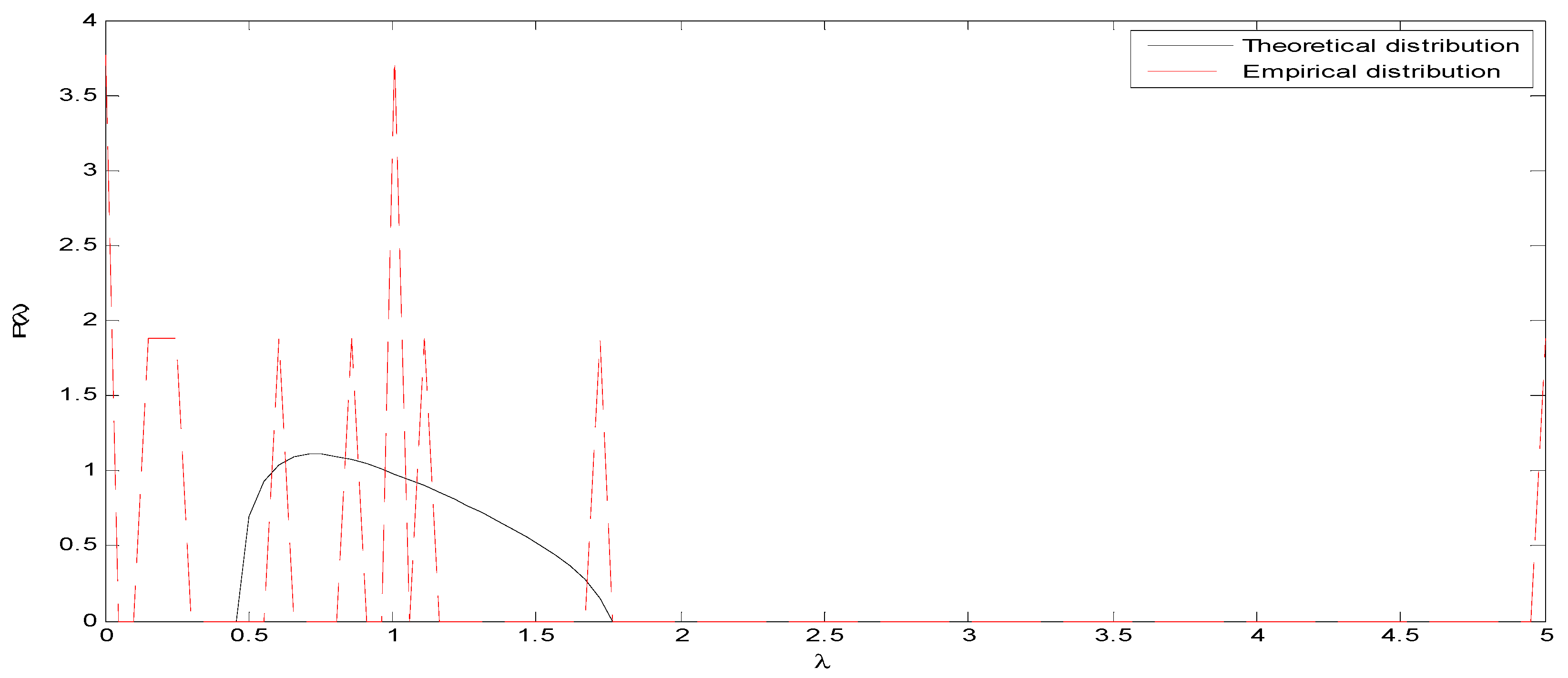
We observe that there are deviations from the interval of eigenvalues $\left[{\lambda }_{-},{\lambda }_{+}\right]$ predicted by RMT. Then, these deviating values might contain pertinent information, and therefore they are not noisy elements.

It is found that theoretical eigenvalues bounds (maximum and minimum) are ${\lambda }_{max}=1.7395$ and ${\lambda }_{min}=0.4639$. We have 12 $\left(N\right)$ series and 118 $\left(L\right)$ monthly returns for each equity. Then, the value of $Q$ is equal to $\frac{L}{N}=9.8333$.

By analyzing results, we observed in Figure 1 that many eigenvalues deviate from RMT interval of predictions. Laloux et al. (2000) found that there is less than $6\%$ of eigenvalues that might contain pertinent information. In our case, these deviations represent $8.33\%$ of the total of eigenvalues, which is a very important percentage. Then, only $91.67\%$ of eigenvalues deals with random matrix theory distribution. Moreover, the maximum of empirical value of eigenvalues $\left({\lambda }_1=5.0374\right)$ exceeds what is predicted by random matrix theory ${\lambda }_{max}=1.7395$.

4.3. Regression Analysis

In the following, we present the results from regressing the University of Michigan Consumer Sentiment Index on the various independent variables.

Table 2. Results of regression analysis—base model.

Dependent Variable: University of Michigan Consumer Sentiment Index
Linear Regression Model 1		Linear Regression Model 2
Undifferentiated Variables	OLS Coefficients	Differentiated Variables	OLS Coefficients
CONSTANT	−0.004706	CONSTANT	0.0004816
BSTARTUP GLOBAL INDEX	0.008914 ‡	BSTARTUP GLOBAL INDEX (-1)	−0.058823
BUSINESS CONFIDENCE INDEX	2.172408 ‡	BUSINESS CONFIDENCE INDEX (-1)	5.759300 **
DOW JONES SUSTAINABILITY US INDEX	−0.283084	DOW JONES SUSTAINABILITY (-1)	1.048775 ***
MSCI GLOBAL ENERGY EFFICIENCY INDEX	−0.317548	MSCI GLOBAL ENERGY EFFICIENT INDEX (-1)	−0.699981 ***
MSCI USA LEADERS INDEX	2.048021 **	MSCI USA LEADERS INDEX (-2)	−0.427186
PI IN BILLIONS	−0.104973	PI IN BILLIONS (-4)	−1.231945 **
SP500 CARBON EFFICIENT	−1.135460	SP 500 CARBON EFFICIENT (-2)	0.643324
SP CONSUMER FINANCE INDEX	0.077979	SP CONSUMER FINANCE_INDEX (−3)	−0.274214 **
SP MUNICIPAL BOND EDUCATION	−0.125058	SP MUNICIPAL BOND EDUCATION (-2)	0.524653
UNEMPLOYMENT RATE IN %	−0.447830 **,‡	UNEMPLOYMENT RATE IN % (-3)	0.318304 *
Adjusted R-squared	0.071882	Adjusted R-squared	0.234387
Sum squared resid	0.203433	Sum squared resid	0.161595
F-statistic	1.906158	F-statistic	4.459419
Prob(F-statistic)	0.051960	Prob(F-statistic)	0.000032

Note: *, **, *** denote significance at 10%, 5%, and 1% levels, respectively. ‡ denotes series that follows a normal distribution according to the Jarque Bera Test (Jarque and Bera 1980).

presents the results from the ordinary least squares (OLS) linear regression for the undifferentiated variables (Model 1) and the differentiated variables (Model 2). In both models, the F-statistic is significant, suggesting that all the independent variables jointly can influence the University of Michigan Consumer Sentiment Index. We observe in Model 1 that only two variables are significant at the level of 5% and the adjusted R-squared represents about 7% of the explained variance. The MSCI USA Leaders Index is significant at the 5% level and that companies with high Environmental, Social, and Governance (ESG) performance contribute positively and importantly in the improvement of the U.S. consumer sentiment. In Model 2, the adjusted R-squared is 23.43% of the explained variance, and six variables are significantly related to the University of Michigan Consumer Sentiment Index. These are Business Confidence Index (-1), Dow Jones Sustainability Index (-1), MSCI Global Energy Efficiency (-1), Personal income (-4), SP Consumer Finance Index (-3), and Unemployment rate (-3). Besides, the adjusted R-squared improved from 7.18% to 23.43% of the explained variance. Model 2 could only be used for predictions given that the differentiations were done iteratively until we got the best results. Overall, some of our results are in line with Lahiri and Zhao (2016), who showed that macroeconomic conditions can explain the sentiment of U.S. consumers.

Next, we split the full sample period into two equal sub-periods to assess whether the estimated model maintains the same predictive power. The related results are given in

Table 3. Results of regression analysis—sub-periods.

Dependent Variable: University of Michigan Consumer Sentiment Index
Variables (First Sub-Period)	OLS Coefficients	Variables (Second Sub-Period)	OLS Coefficients
CONSTANT	0.011538	CONSTANT	−0.000718
BSTARTUP GLOBAL INDEX (-1)	−0.185552 **	BSTARTUP GLOBAL INDEX (-1)	0.041828
BUSINESS CONFIDENCE INDEX (-1)	7.983167 *	BUSINESS CONFIDENCE INDEX (-1)	3.726710
DOW JONES SUSTAINABILITY (-1)	1.420353 ***	DOW JONES SUSTAINABILITY (-1)	0.538998 *
MSCI GLOBAL ENERGY EFFICIENT INDEX (-1)	−1.024799 ***	MSCI GLOBAL ENERGY EFFICIENT INDEX (-1)	−0.294351
MSCI USA LEADERS INDEX (-2)	0.206585	MSCI USA LEADERS INDEX (-2)	−1.348939
PI IN BILLIONS (-4)	−1.420226 *	PI IN BILLIONS (-4)	−0.342955
SP 500 CARBON EFFICIENT (-2)	0.093590	SP 500 CARBON EFFICIENT (-2)	1.342124
SP CONSUMER FINANCE_INDEX (-3)	−0.408050 **	SP CONSUMER FINANCE_INDEX (-3)	−0.085687
SP MUNICIPAL BOND EDUCATION (-2)	0.538481	SP MUNICIPAL BOND EDUCATION (-2)	0.514044
UNEMPLOYMENT RATE IN % (-3)	0.765796 **	UNEMPLOYMENT RATE IN % (-3)	−0.224393
Adjusted R-squared	0.372938	Adjusted R-squared	0.015380
Sum squared resid	0.084147	Sum squared resid	0.054434
F-statistic	4.211591	F-statistic	1.090595
Prob(F-statistic)	0.000000	Prob(F-statistic)	0.388141

Note: *, **, *** denote significance at 10%, 5%, and 1% levels, respectively.

. Notably, they show the significance of seven variables in the first sub-period compared to only one variable in the second sub-period. The Adjusted R-squared is 37% in the first sub-period and 1.5% in the second sub-period. Accordingly, we can say that the model is not stable over time since it shows very different results in each sub-period. This suggests the need to move beyond the linear regression in order to capture nonlinearity in the model.

4.4. Regime Switching Model

We applied the regime-switching model (Hamilton 2005), which is used in previous studies (e.g., Geng et al. 2016).

For one variable, the typical behavior could be described with a first autoregression as follows,

$$y_t=c_1+\varnothing y_{t-1}+{\epsilon }_t$$

with ${\epsilon }_t~N\left(0,{\sigma }^2\right)$, which seemed to be adequately the observed data for $t=1, 2, \dots ,t_0$.

$t_0$ is a date where there is a significant change in the average of the series, so that instead the data would be described as follows,

$$y_t=c_2+\varnothing y_{t-1}+{\epsilon }_t$$

for $t=t_0+1, t_0+2, \dots$ This fix of changing the value of the intercept from $c_1$ to $c_2$ might help the model to get back on track with better forecasts, but it is rather unsatisfactory as a probability law that could have generated the data.

Rather than claim that the first equation above governed the data up to date $t_0$ and the second one after that date, it is possible to write that in one equation,

$$y_t=c_{s_t}+\varnothing y_{t-1}+{\epsilon }_t$$

where $s_t$ is a random variable, as a result of institutional changes that happened in the sample.

$s_t=1$ for $t=1, 2, \dots , t_0$ and $s_t=2$ for $t=t_0+1, t_0+2, \dots$

The probabilistic model of what caused the change from $s_t=1$ to $s_t=2$ where $s_t$ is the realization of a two-state Markov chain with

$$\mathrm{Pr}\left(s_t=j|s_{t-1}=k,\dots , y_{t-1},y_{t-2},\dots \right)=\mathrm{Pr}\left(s_t=j|s_{t-1}=i\right)=p_{ij}$$

$s_t$ is not supposed to be observed directly, but only infer its operation though the observed behavior $y_t$. The probability of a change in regime depends on the past only through the value of the most recent regime (Hamilton 2005). Furthermore, if the regime change reflects a fundamental change in monetary or fiscal policy, the prudent assumption would seem to be to allow the possibility for it to change back again, suggesting that $p_{22}<1$ is often a more natural formulation for thinking about changes in regime than $p_{22}=1$ (Hamilton 2005). We present in

Table 4. Results of regression analysis—Regime-Switching model.

Dependent Variable: University of Michigan Consumer Sentiment Index
Variables	RS Coefficients (Regime 1)	RS Coefficients (Regime 2)
CONSTANT	0.010338 *	−0.011795
BSTARTUP GLOBAL INDEX	−0.025739	−0.027302
BUSINESS CONFIDENCE INDEX	−1.263362	12.07068 **
DOW JONES SUSTAINABILITY	0.752385	−0.751735
MSCI GLOBAL ENERGY EFFICIENCY	−0.272709	−0.638802 *
MSCI USA LEADERS INDEX	0.322006	3.966401 ***
PI IN BILLIONS	0.191583	−4.290645 ***
SP 500 CARBON EFFICIENT	−1.077221	−1.702474
SP CONSUMER FINANCE_INDEX	0.471282 **	−0.355529
SP MUNICIPAL BOND EDUCATION	0.842489 *	−2.616637 ***
UNEMPLOYMENT RATE IN %	−0.397643 **	−0.381531
Sum squared resid	0.212884
Probabilities Parameters	0.774284 | 0.427532 | 1.811054 | 0.0701

Note: *, **, *** denote significance at 10%, 5%, and 1% levels, respectively.

the results of the regime-switching model.

Results from Regime 1 show that the SP Municipal Bond Education is statistically significant at 10%, reflecting the positive impact of the student loan on the University of Michigan Consumer Sentiment Index. The SP Consumer Finance index and unemployment rate are also significant at the level of 5%. The SP Consumer Finance Index contributes significantly and positively to the consumer sentiment index, while the unemployment rate contributes negatively to it. In that state (1), the U.S. consumer seems to be frustrated about the other variables and then has less confidence in sustainability variables, innovation freedom, energy efficiency policies, and personal income expectations. However, MSCI Global Energy Efficiency, SP Municipal Bond Education, and Personal Income contribute negatively to the level of the University of Michigan Consumer Sentiment Index after switching from Regime 1 to Regime 2. This result should be explained as an important change in the social and economic state in the U.S. Furthermore, other variables become significant; Business Confidence Index and MSCI USA Leaders Index have a significant and positive impact. This can be explained by the fact that the improvement of businesses affects directly and positively the consumer sentiment. As for the positive impact of the MSCI USA Leaders Index, it can be explained by the fact that U.S. consumers are highly satisfied by the Environmental, Social, and Governance (ESG) performance of companies belonging to the MSCI USA Leaders Index. Finally, personal income shows a negative relationship with the University of Michigan Consumer Sentiment Index.

Based on the above results, we indicate that the regime-switching model presents a switch from a state one where U.S. consumers were not confident about the variables studied in relation to sustainability, personal income, environment, and business confidence to state two, when there was a switch towards more confidence and more positive sentiment regarding energy efficiency, unemployment rate, student loan, sustainability, and business confidence.

Furthermore, results from

Table 5. Constant simple transition probabilities and constant expected durations of the regime-switching regression.

Constant Simple Transition Probabilities
$P\left(i,k\right)=P(s\left(t\right)=k|s\left(t-1\right)=i)$
$\left(row=i/column=j\right)$
	1	2
1	0.684446	0.315554
2	0.684446	0.315554
Constant Expected Durations
	1	2
	3.169033	1.461035

show that the probabilities of being in Regime 1 are more than 68% while the probabilities of being in Regime 2 are 31.56%. We also observe that both probabilities do not depend on the origin state. The constant expected duration is also higher in Regime 1 with a duration of 3.17 months, compared to only 1.47 months in Regime 2. Accordingly, U.S. consumers seem to stay most of the time in Regime 1 and are usually less confident in sustainability variables, innovation freedom, energy efficiency policies, and personal income expectations. The switch to Regime 2 is seasonal and depends on the social, economic, political, and institutional mutations in the U.S.

4.5. Gradient Descent Algorithm

We computed a gradient descent for the linear regression in order to compare the results obtained. The gradient descent is an optimization algorithm used to minimize a function by iteratively moving in the direction of steepest descent, as defined by the negative of the gradient (Cauchy 1847). Algorithms play an important role in the optimization process. They are defined as a finite sequence of well-defined, computer-implementable instructions, in order to solve a class of problems or to perform a computation. Gradient descent will allow us to update linear regression coefficients in an iterative way until convergence. Then, we will try to minimize the function of mean squared error (cost function) that is considered as the difference between the estimator and the estimated values.

$$Mean Squared Error=\frac{1}{N}{\displaystyle \sum }_{i=1}^n{(Y_i-{\widehat{Y}}_i)}^2$$

The adjustment of this equation allows for making a calculation simpler with the Gradient Descent Algorithm to obtain the following equation,

$$Mean Squared Error=\frac{1}{2m}{\displaystyle \sum }_{i=1}^m{(h_{\theta }(x^{(i)})-y^{(i)})}^2$$

Gradient Descent changes the theta values iteratively until, in a way, that minimizes the cost function. We start the algorithm by initializing theta (0) and theta (1).

$${\theta }_j≔{\theta }_j-\alpha \frac{\partial }{\partial {\theta }_i}J({\theta }_0,{\theta }_1)\hspace{1em}\hspace{1em}(for j=0 and j=1)$$

where α, alpha, is the learning rate, or how quickly we want to move towards the minimum. If α is too large, however, we can overshoot.

The algorithm will be repeated until convergence

$$\{{\theta }_0≔{\theta }_0-\alpha \frac{1}{m}{\displaystyle \sum }_{i=1}^m(h_{\theta }(x^{(i)})-y^{(i)})$$

$${\theta }_1≔{\theta }_1-\alpha \frac{1}{m}{\displaystyle \sum }_{i=1}^m(h_{\theta }(x^{(i)})-y^{(i)})·x^{\left(i\right)}\}$$

After computing the algorithm, we obtained the results presented in

Table 6. Results involving the Gradient Descent Algorithm.

Number of iterations: 2000
Error tolerance for Theta: 0.05
Tolerance for the cost function: 0.05
Initial guess for Theta: zeros (1, 11)
Learning rate for gradient descent algorithm: 0.1
Error = 0.00076494
Least-square estimate of Theta:
Theta = 0.001
0.0917 0.2379 0.3196 0.2878 0.3837 −0.0344 0.0101 0.0702 −0.0015 −0.2995 0.3034

Note: The table shows the number of iterations used in order to run the Gradient Descent Algorithm, we chose an error tolerance and tolerance for the cost function that are equal to 0.05. The learning rate was set at 0.1. The results show that the error was minimized to 0.001 after computing the coefficient of each variable.

.

We can see that the sum of errors computed by using Gradient Descent Algorithm is smaller than the one found in the other ordinary linear regressions and the switching regime model. The interpretation of the coefficient is not possible since this learning machine algorithm aims to minimize the cost function regardless of the meaning of the coefficients. Thus, this model could be used to do predictions that are more accurate since it has less errors comparing to the other models computed above and gives it a high predictive power.

5. Conclusions

In this paper, we examined the relationship between the U.S. consumer sentiment and other relevant financial indexes in relation to education, environment, sustainability, and innovation freedom. We started by analyzing all the variables structure via cross-correlation and RMT analysis. Results show that more than 8.33% of the total of eigenvalues contain deviate from the RMT and contain then pertinent information, which means that those variables are useful for our analysis. Then, we used the linear regression which fails to capture the nonlinearity interaction among the variables, especially after estimating the linear regression in two equal sub-periods. Accordingly, we employed the regime-switching regression, and the results show that the model presents a switch from a Regime 1 where U.S. consumers were not confident about the variables studied in relation to sustainability, personal income, environment, and business confidence, to Regime 2, where there was a switch towards more confidence and more positive sentiment regarding energy efficiency, unemployment rate, student loan, sustainability, and business confidence. However, U.S. Consumers stay most of the time in Regime 1 and are usually less confident in sustainability variables, innovation freedom, energy efficiency policies, and personal income expectations. The switch to Regime 2 is seasonal and depends on the social, economic, political and institutional mutations in the U.S. Finally, we computed the Gradient Descent Algorithm to compare the errors obtained in each model. We found that the algorithm gives less error and could be used to do better predictions comparing to the other models with a high predictive power.

Our analyses and results extend our limited understanding regarding the exogenous factors that determine the U.S. consumer sentiment and the suitability of prediction models. In fact, we have shown that noneconomic and nonfinancial variables matter to the level of the U.S. consumer sentiment and that nonlinear models combined with Gradient Descent Algorithm have a more significant prediction power over standard regression models.

Our results have policy implications given that the findings presented above improve our understanding of the factors driving the sentiment of U.S. consumers. The results can be useful to investors in a way that would help them better understand the drivers of the U.S. consumers’ sentiment and the overall level of confidence in the U.S. economy. Furthermore, the results have implications regarding consumption, saving, investment, and other related variables. Consumers can benefit from the findings to enhance their understanding of the most important problems that are impacting their sentiments, which might induce economic, social, and political consequences through voting decisions or economic and social adjustments. For policymakers, there seems to be a possibility to design policies capable of exploiting the association between current economic and stock markets conditions and consumers’ confidence. Given the significant role played by specific factors, a practical policy formulation is merited to enhance U.S. consumer confidence with appropriate initiatives that involve education, environment, sustainability, and innovation freedom. If employed, such policies can enhance the well-being of the U.S. consumers.

Future studies can consider conducting an analysis that involves various developed and emerging countries. Another extension could be the application of a mixed-data sampling to exploit the high frequency of data on stock indices in explaining consumer confidence.

References

- Akhtar, Shumi, Robert Faff, Barry Oliver, and Avanidhar Subrahmanyam. 2011. The power of bad: The negativity bias in Australian consumer sentiment announcements on stock returns. Journal of Banking & Finance 35: 1239–49. [Google Scholar]
- Baghestani, Hamid, and Polly Palmer. 2017. On the dynamics of US consumer sentiment and economic policy assessment. Applied Economics 49: 227–37. [Google Scholar] [CrossRef]
- Balcilar, Mehmet, Rangan Gupta, and Clement Kyei. 2018. Predicting Stock Returns and Volatility with Investor Sentiment Indices: A Reconsideration Using a Nonparametric Causality-In-Quantiles Test. Bulletin of Economic Research 70: 74–87. [Google Scholar] [CrossRef] [Green Version]
- Baker, Malcolm, and Jeffrey Wurgler. 2006. Investor Sentiment and the Cross-Section of Stock Returns. The Journal of Finance 61: 1645–80. [Google Scholar] [CrossRef] [Green Version]
- Baker, Malcolm, and Jeffrey Wurgler. 2007. Investor Sentiment in the Stock Market. Journal of Economic Perspectives 21: 129–51. [Google Scholar] [CrossRef] [Green Version]
- Bouchaud, Jean-Philippe, and Marc Potters. 2003. Theory of Financial Risk and Derivative Pricing: From Statistical Physics to Risk Management. Cambridge: Cambridge University Press. [Google Scholar]
- Bouteska, Ahmed. 2019. The effect of investor sentiment on market reactions to financial earnings restatements: Lessons from the United States. Journal of Behavioral and Experimental Finance 24: 1–11. [Google Scholar] [CrossRef]
- Cauchy, Augustin. 1847. Méthode générale pour la résolution des systèmes d’équations simultanées. Comptes rendus de l’Académie des Sciences 25: 536–38. [Google Scholar]
- Chung, San-Lin, Chi-Hsiou Hung, and Chung-Ying Yeh. 2012. When does investor sentiment predict stock returns? Journal of Empirical Finance 19: 217–40. [Google Scholar] [CrossRef]
- Cofnas, Abe, ed. 2015. How Business Confidence and Consumer Sentiment Affect the Market. In The Forex Trading Course: A Self-Study Guide to Becoming a Successful Currency Trader. Hoboken: John Wiley & Sons Inc., pp. 51–52. [Google Scholar]
- Dyson, Freeman J. 1971. Distribution of eigenvalues for a class of real symmetric matrices. Revista Mexicana de Fisica 20: 231–37. [Google Scholar]
- Fisher, Kenneth L., and Meir Statman. 2000. Investor Sentiment and Stock Returns. Financial Analyst Journal 56: 16–23. [Google Scholar] [CrossRef]
- Fisher, Lance A., and Hyeon-seung Huh. 2016. On the econometric modelling of consumer sentiment shocks in SVARs. Empirical Economics 51: 1033–51. [Google Scholar] [CrossRef]
- Geng, Jiang-Bo, Qiang Ji, and Ying Fan. 2016. The impact of the North American shale gas revolution on regional natural gas markets: Evidence from the regime-switching model. Energy Policy 96: 167–78. [Google Scholar] [CrossRef]
- Gupta, Rangan, Shawkat Hammoudeh, Mampho P. Modise, and Duc Khuong Nguyen. 2014. Can economic uncertainty, financial stress and consumer sentiments predict US equity premium? Journal of International Financial Markets, Institutions and Money 33: 367–78. [Google Scholar] [CrossRef] [Green Version]
- Hamilton, James D. 2005. Regime-Switching Models. In Macroeconometrics and Time Series Analysis. The New Palgrave Economics Collection. London: Palgrave Macmillan, pp. 2002–209. [Google Scholar]
- Issa, Mohamed H., Joseph H. Rankin, Mohamed Attalla, and John A. Christian. 2011. Absenteeism, performance and occupant satisfaction with the indoor environment of green Toronto schools. Indoor and Built Environment 20: 511–53. [Google Scholar] [CrossRef]
- Jarque, Carlos M., and Anil K. Bera. 1980. Efficient tests for normality, homoscedasticity and serial independence of regression residuals. Economics Letters 6: 255–59. [Google Scholar] [CrossRef]
- Kurov, Alexander. 2008. Investor Sentiment, Trading Behavior and Informational Efficiency in Index Futures Markets. The Financial Review 43: 107–27. [Google Scholar] [CrossRef]
- Lahiri, Kajal, and Yongchen Zhao. 2016. Determinants of consumer sentiment over business cycles: Evidence from the US surveys of consumers. Journal of Business Cycle Research 12: 187–215. [Google Scholar] [CrossRef] [Green Version]
- Laloux, Laurent, Pierre Cizeau, Jean-Philippe Bouchaud, and Marc Potters. 1999. Noise Dressing of Financial Correlation Matrices. Physical Review Letters 83: 1467–70. [Google Scholar] [CrossRef] [Green Version]
- Laloux, Laurent, Pierre Cizeau, Marc Potters, and Jean-Philippe Bouchaud. 2000. Random Matrix Theory and financial correlations. International Journal of Theoretical and Applied Finance 3: 1–6. [Google Scholar] [CrossRef]
- Pafka, Szilard, and Imre Kondor. 2004. Estimated correlation matrices and portfolio optimization. Physica A: Statistical Mechanics and Its Applications 343: 623–34. [Google Scholar] [CrossRef] [Green Version]
- Paraboni, Ana Luiza, Marcelo Brutti Righi, Kelmara Mendes Vieira, and Vinícius Girardi da Silveira. 2018. The Relationship between Sentiment and Risk in Financial Markets. Brazilian Administration Review 15: e163596. [Google Scholar] [CrossRef] [Green Version]
- Plerou, Vasiliki, Parameswaran Gopikrishnan, Bernd Rosenow, Luis A. Nunes Amaral, Thomas Guhr, and H. Eugene Stanley. 2002. Random matrix approach to cross correlations in financial data. Physical Review E 65: 066126. [Google Scholar] [CrossRef] [PubMed] [Green Version]
- Schmeling, Malik. 2009. Investor sentiment and stock returns: Some international evidence. Journal of Empirical Finance 16: 394–408. [Google Scholar] [CrossRef] [Green Version]
- Sengupta, Anirvan M., and Partha P. Mitra. 1999. Distributions of Singular Values for Some Random Matrices. Physical Review E 60: 3389–92. [Google Scholar] [CrossRef] [Green Version]
- Shahzad, Syed Jawad Hussain, Elie Bouri, Naveed Raza, and David Roubaud. 2019. Asymmetric impacts of disaggregated oil price shocks on uncertainties and investor sentiment. Review of Quantitative Finance and Accounting 52: 901–21. [Google Scholar] [CrossRef]
- Stivers, Adam. 2015. Forecasting returns with fundamentals-removed investor sentiment. International Journal of Financial Studies 3: 319–41. [Google Scholar] [CrossRef] [Green Version]
- van Giesen, Roxanne I., and Rik Pieters. 2019. Climbing out of an economic crisis: A cycle of consumer sentiment and personal stress. Journal of Economic Psychology 70: 109–24. [Google Scholar] [CrossRef]
- Wadud, Mokhtarul, Huson Joher Ali Ahmed, and Xueli Tang. 2019. Factors affecting delinquency of household credit in the US: Does consumer sentiment play a role? The North American Journal of Economics and Finance 52: 101132. [Google Scholar] [CrossRef]
- Zhang, Yue-Jun, and Jia-Min Pei. 2019. Exploring the impact of investor sentiment on stock returns of petroleum companies. Energy Procedia 158: 4079–85. [Google Scholar] [CrossRef]
- Zhou, Guofu. 2018. Measuring investor sentiment. Annual Review of Financial Economics 10: 239–59. [Google Scholar] [CrossRef]
Figure 1.
Theoretical (Marčenko-Pastur) and empirical distributions of eigenvalues.