Analysis of a Chaotic System with Line Equilibrium and Its Application to Secure Communications Using a Descriptor Observer †

 ,
,  ,
, 
 , and
, and 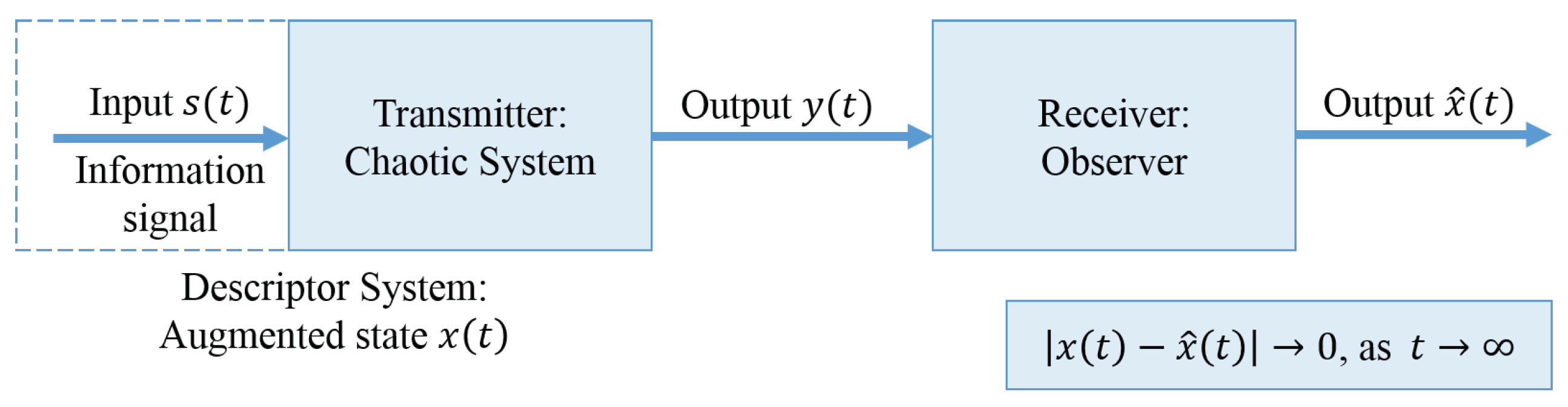
Abstract
:1. Introduction
2. The Proposed Dynamical System
2.1. System Description
- The system has only five terms. Till now only few chaotic 3D dynamical systems with five terms have been reported in literature. Most of them belong to the class of jerk systems and they have been introduced by Professor Sprott and his colleagues [47,48]. However, there are few others, which are written in the general 3D dynamical system’s form [49,50,51,52,53]. In 1997, Fu and Heidel rigorously proved that there can be no simpler system with a quadratic nonlinearity [54].
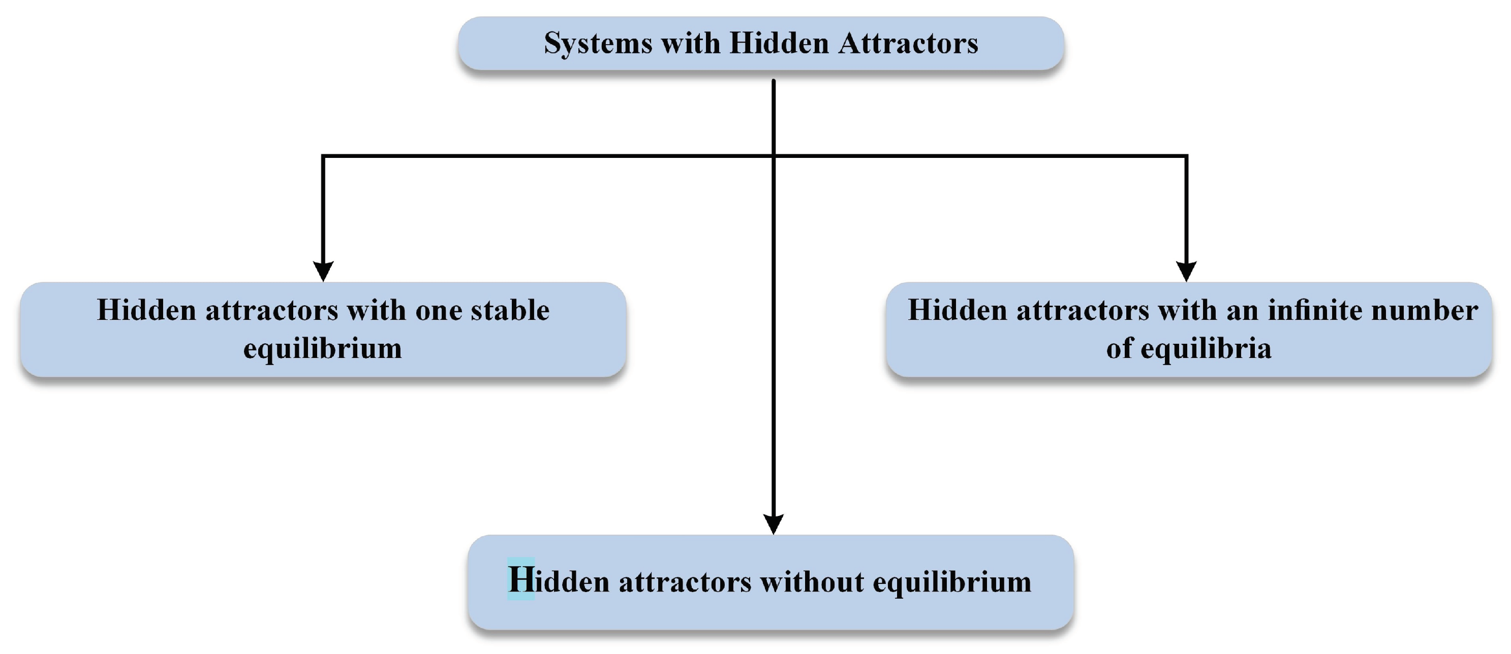
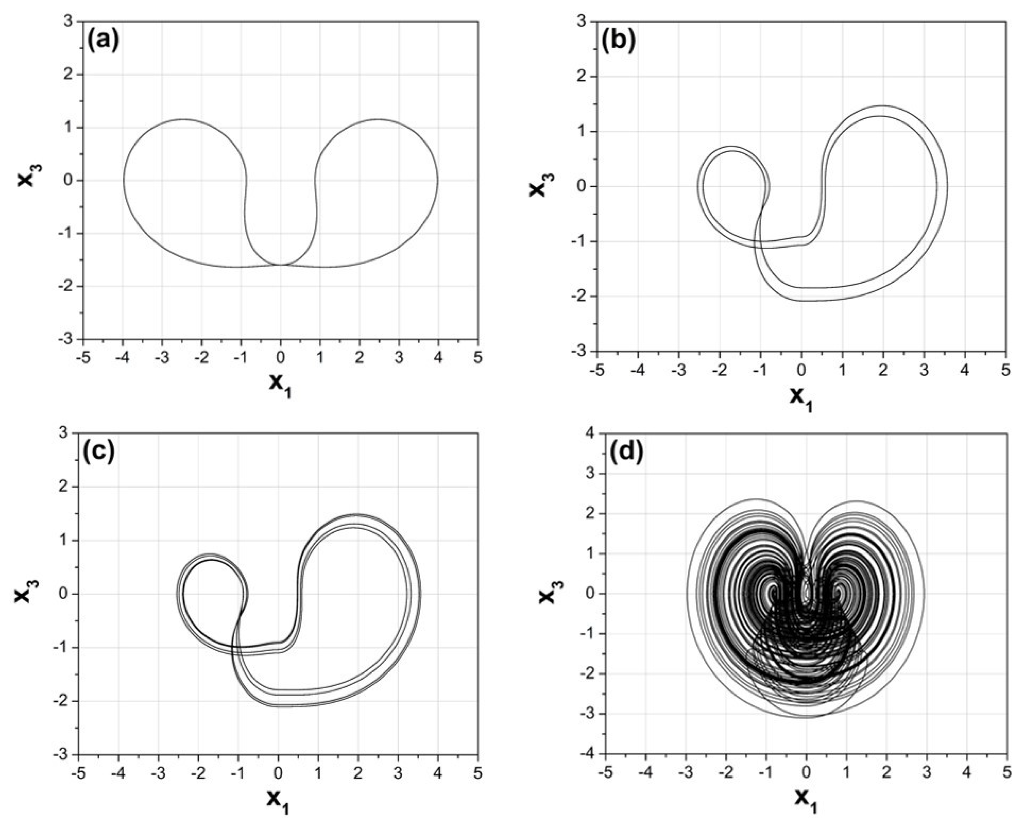
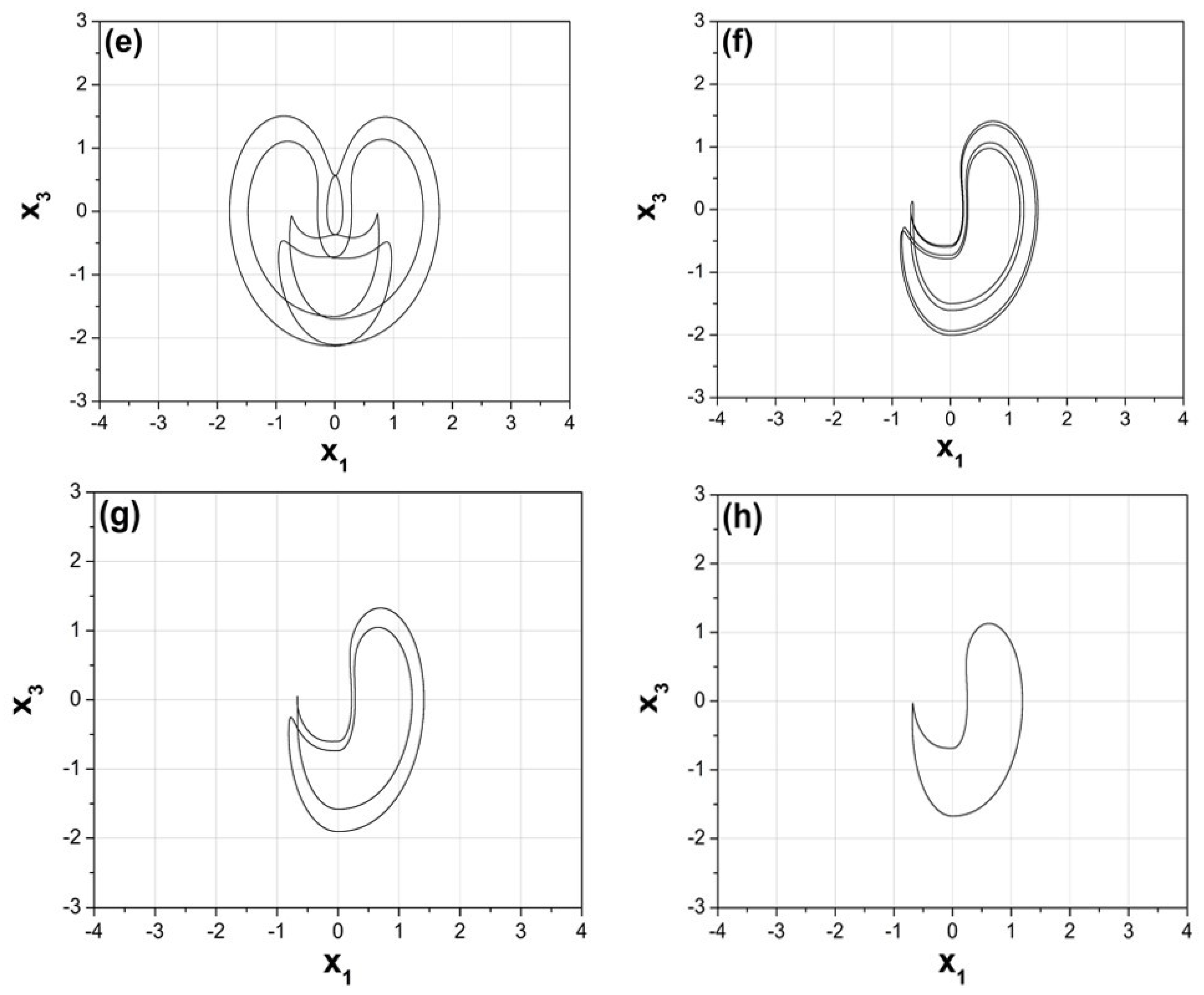
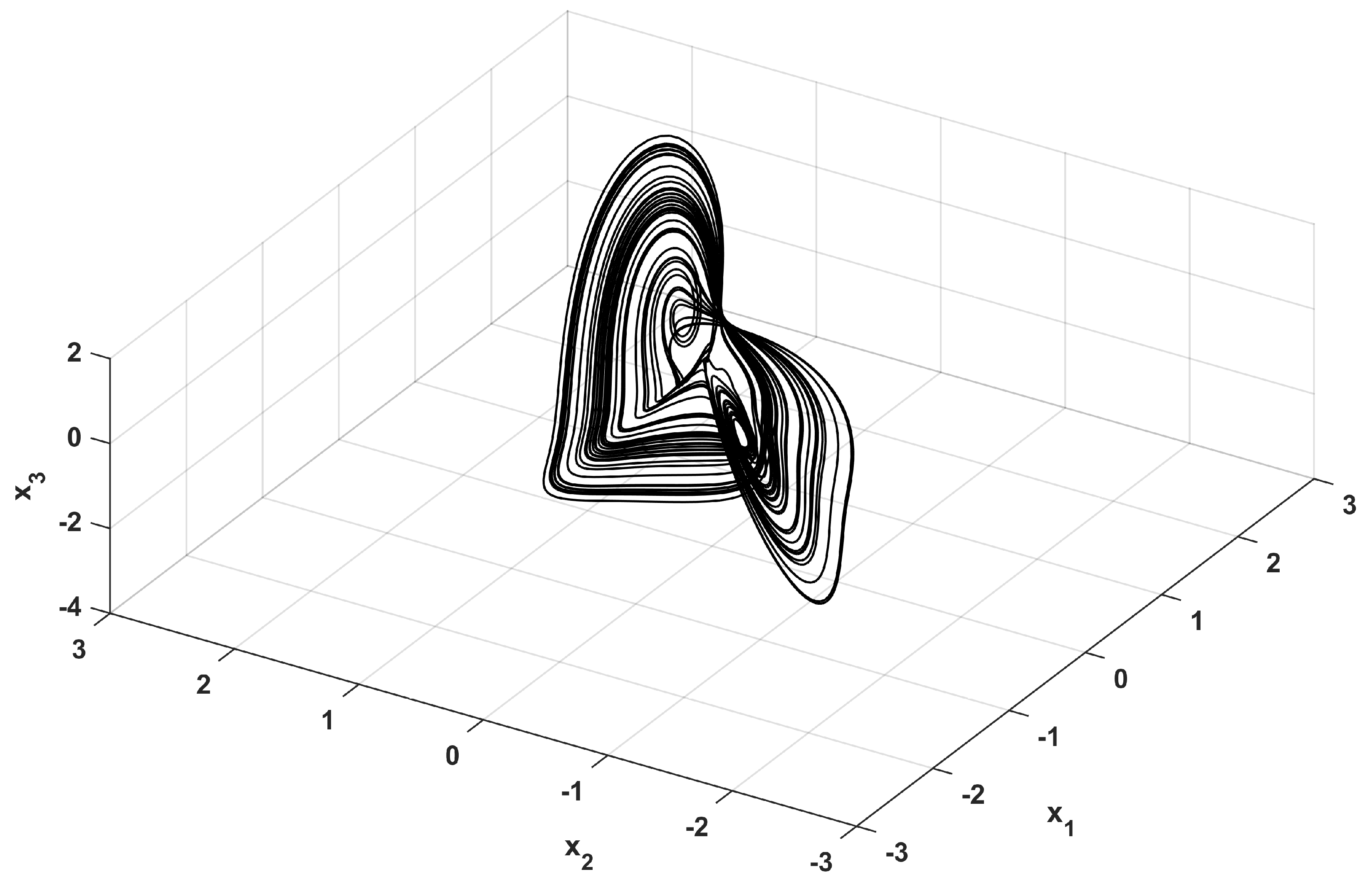
- By solvingIt is easy to verify that (1) has a line of equilibrium points . Therefore, system’s attractor is hidden.
- The amplitude is easily controllable.
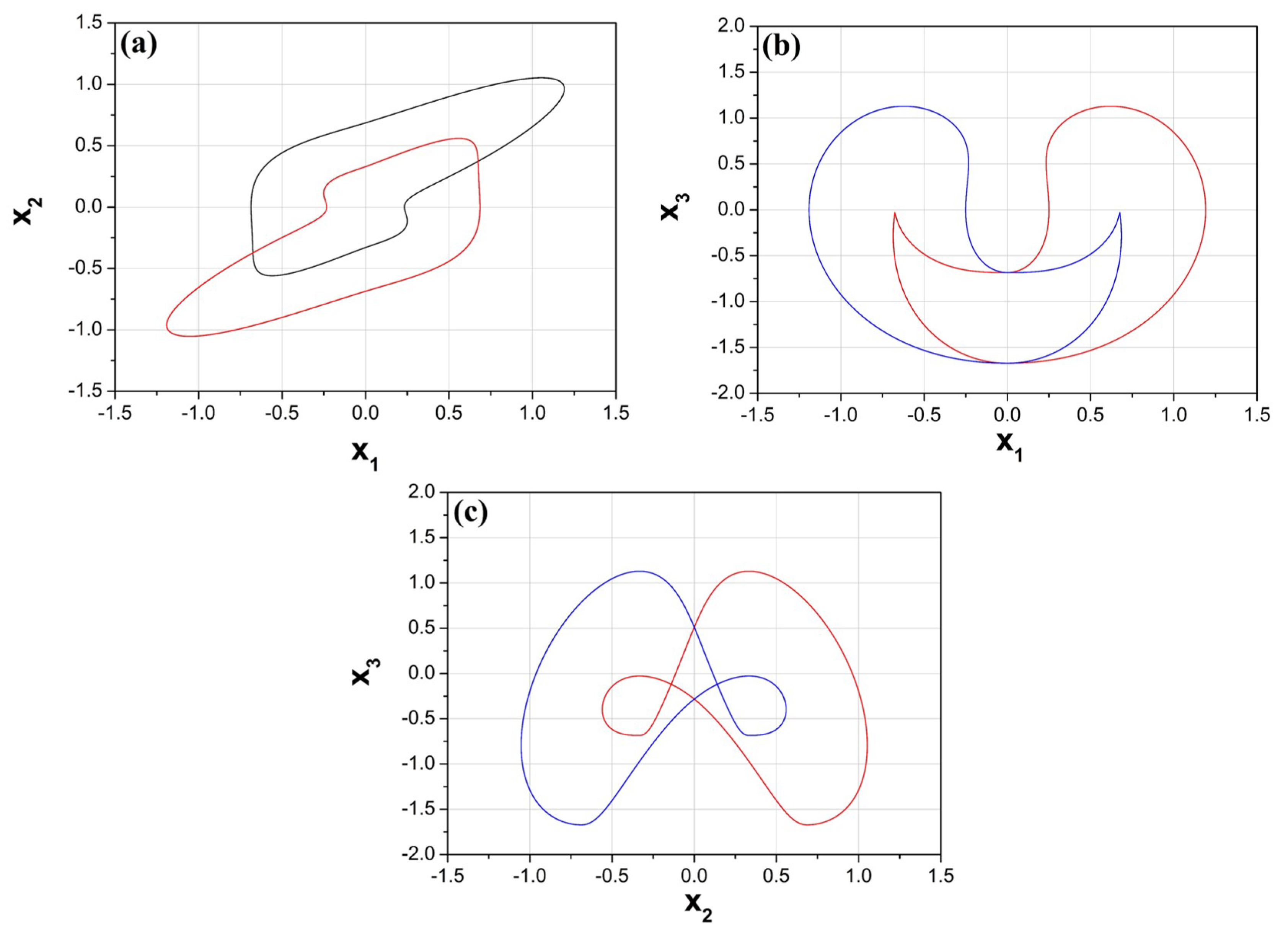
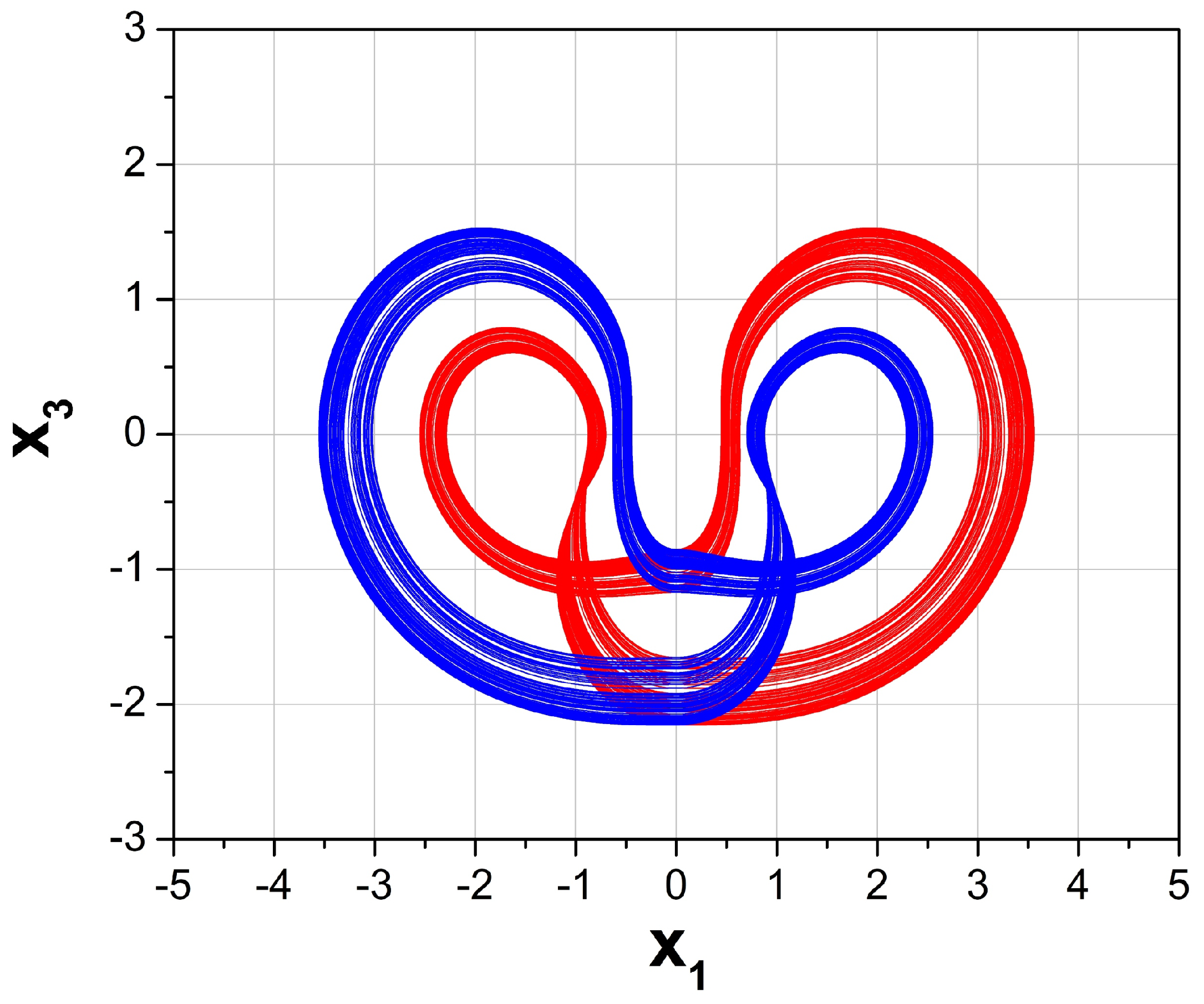
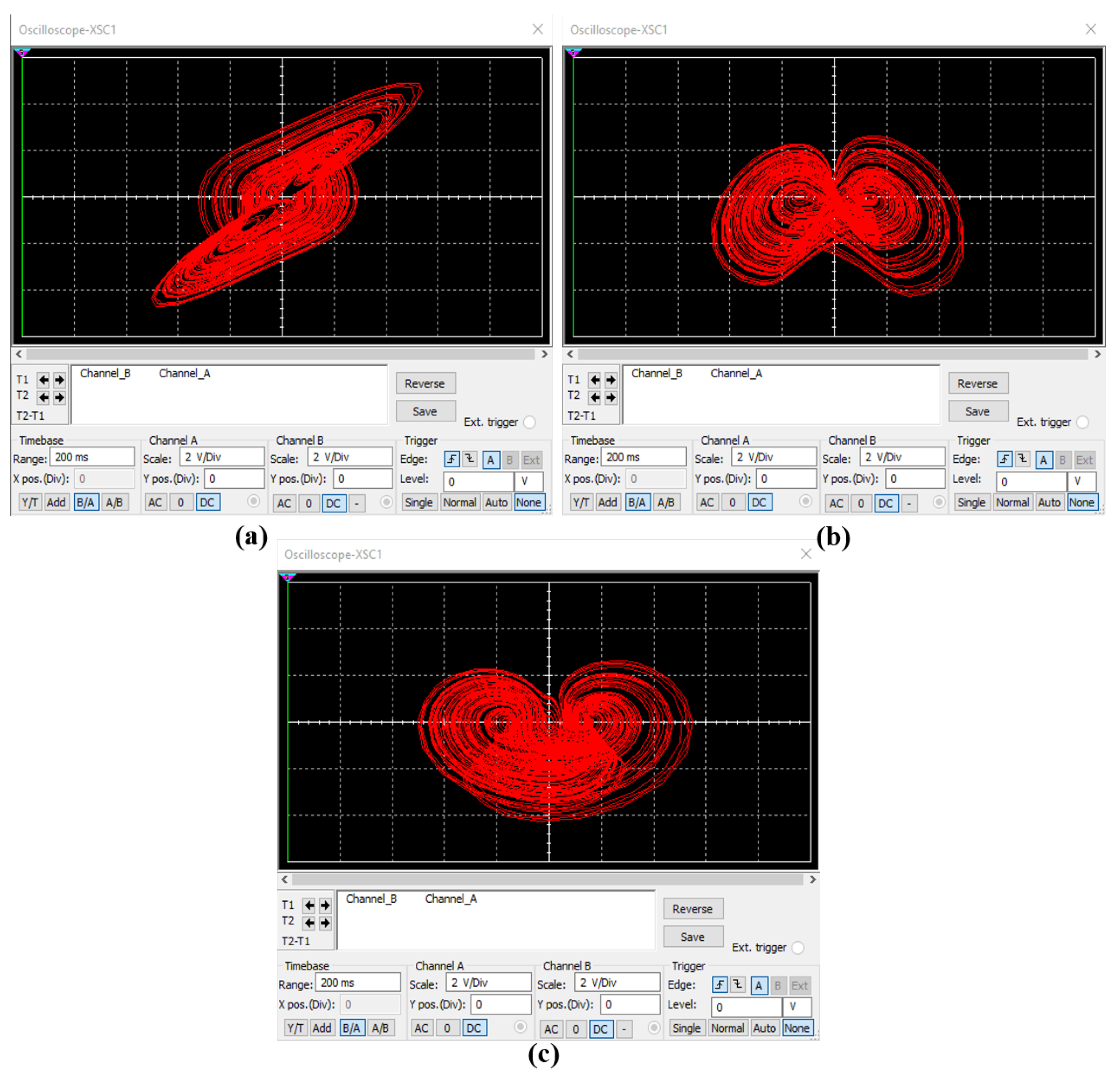
- The system is symmetric through the transformation .This symmetry is observed in Figure 3, where two symmetric system’s periodic attractors, in the three different planes, for and initial conditions , with red color, and , with blue color, has been captured.
2.2. Dynamical Analysis
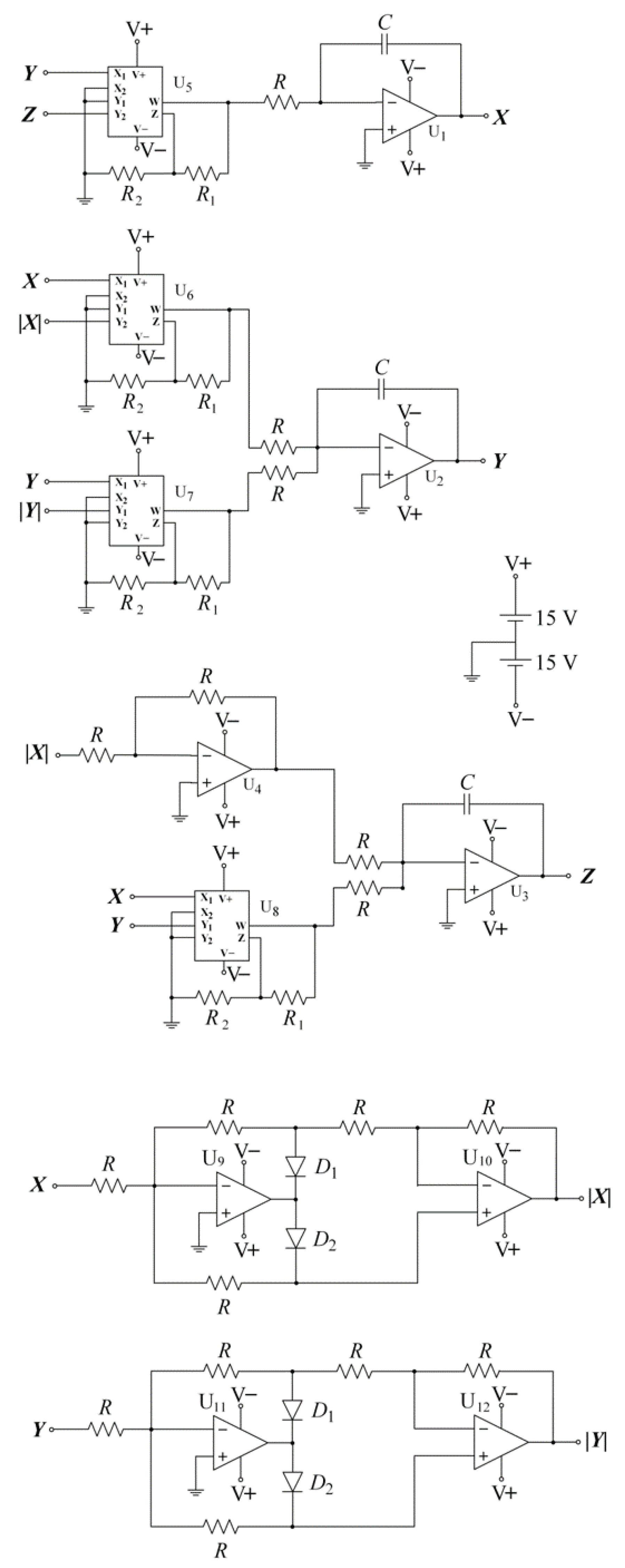
3. Realization of the System
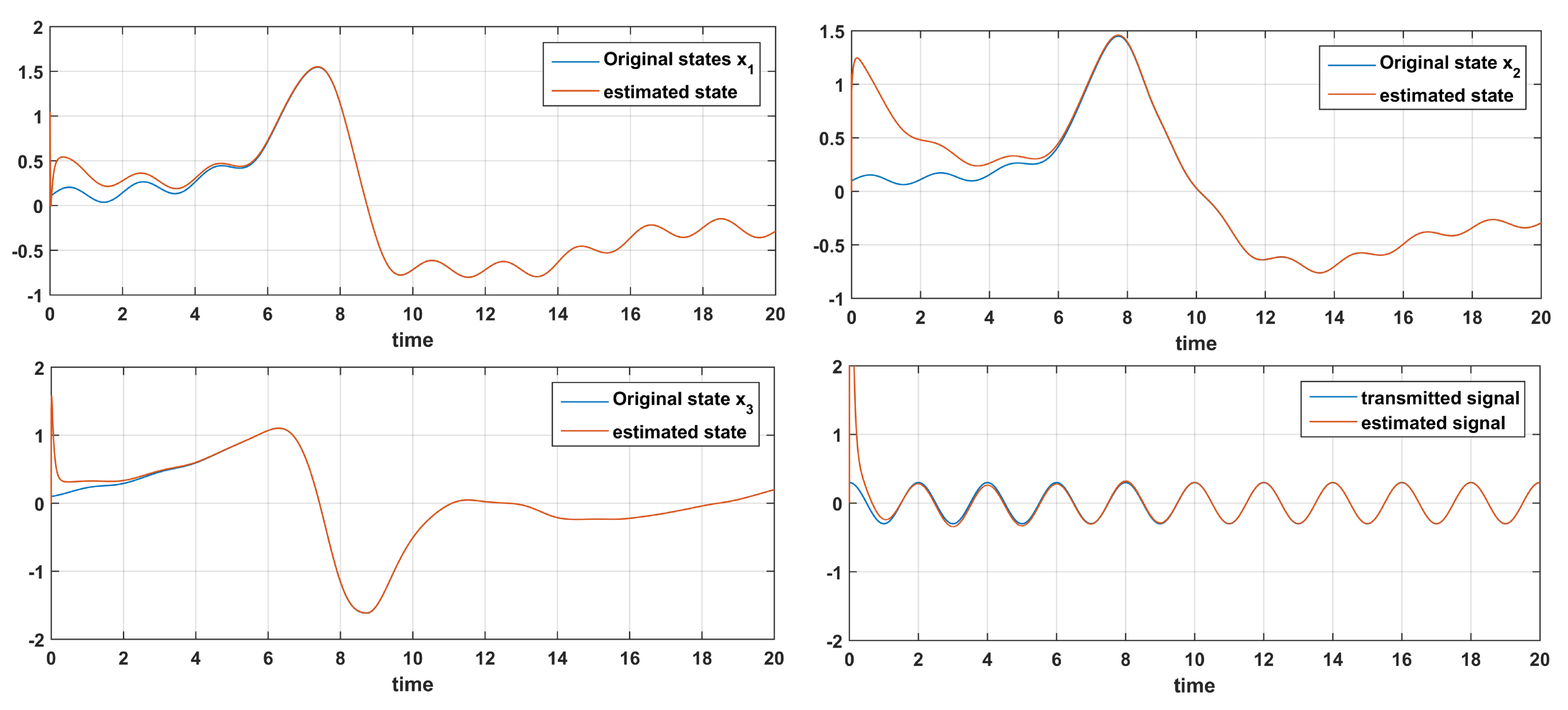
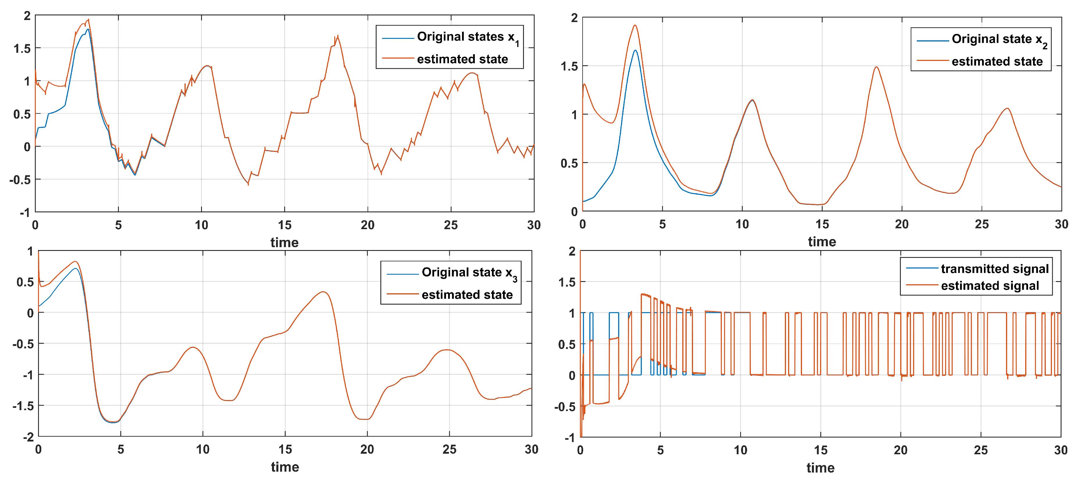
4. Application to Secure Communications
- (A.1)
- , where n is the number of columns of E. So, by considering the form of E, one can see that this is equivalent to D having full column rank.
- (A.2)
- The nonlinear part satisfies the Lipschitz property, that is, there exists a positive scalar such that
- Compute the matrix R, following the procedure given in ([67] Appendix A.)
- Compute the matrices , that correspond to the systemand check the solvability of the LMIfor and .
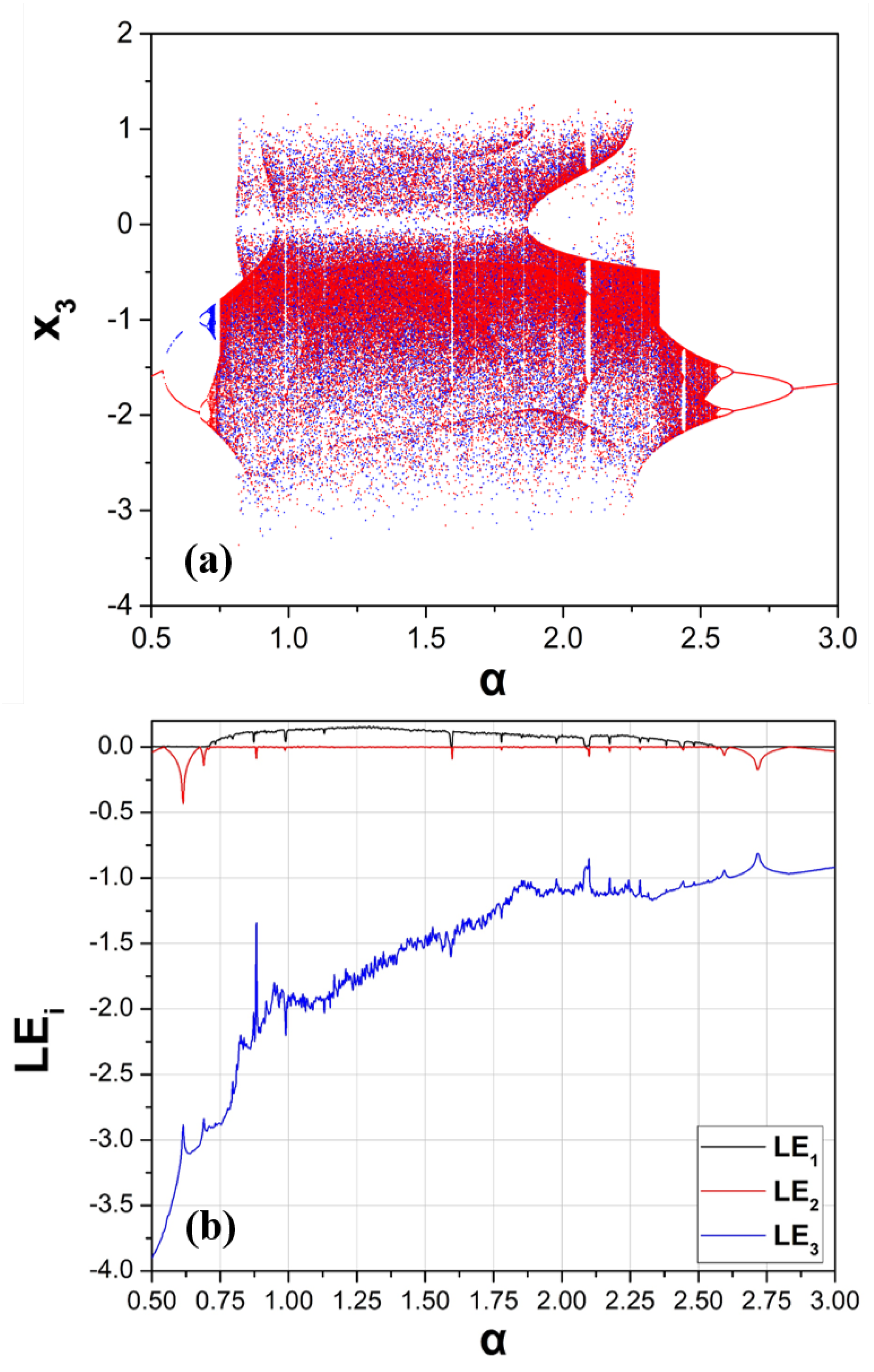
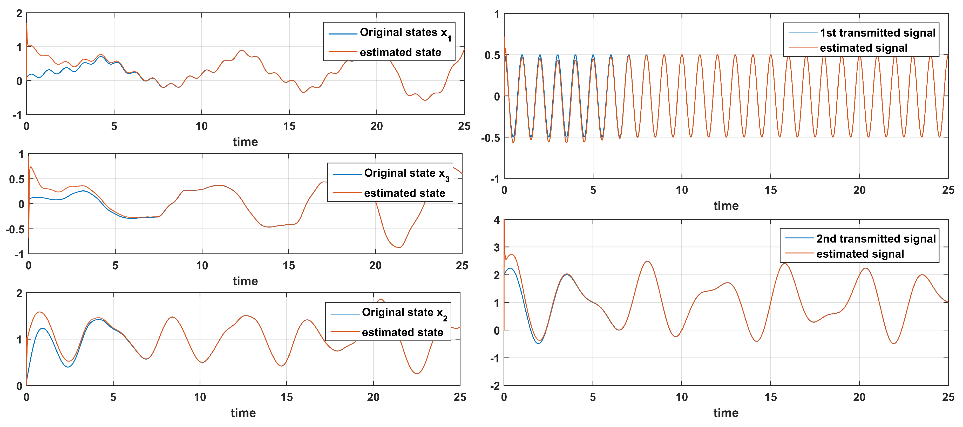
5. Simulation Results
6. Conclusions and Future Aspects
Author Contributions
Funding
Acknowledgments
Conflicts of Interest
References
- Pecora, L.M.; Carroll, T.L. Synchronization in chaotic systems. Phys. Rev. Lett. 1990, 64, 821–824. [Google Scholar] [CrossRef] [PubMed]
- Volos, C.K.; Kyprianidis, I.M.; Stouboulos, I.N. Image encryption process based on chaotic synchronization phenomena. Signal Process. 2013, 93, 1328–1340. [Google Scholar] [CrossRef]
- Xu, Y.; Wang, H.; Li, Y.; Pei, B. Image encryption based on synchronization of fractional chaotic systems. Commun. Nonlinear Sci. Numer. Simul. 2014, 19, 3735–3744. [Google Scholar] [CrossRef]
- Tirandaz, H.; Karmi-Mollaee, A. Modified function projective feedback control for time-delay chaotic Liu system synchronization and its application to secure image transmission. Optik 2017, 147, 187–196. [Google Scholar] [CrossRef]
- Yang, T. A survey of chaotic secure communication systems. Int. J. Comput. Cogn. 2004, 2, 81–130. [Google Scholar]
- Martínez-Guerra, R.; García, J.J.M.; Prieto, S.M.D. Secure communications via synchronization of Liouvillian chaotic systems. J. Frankl. Inst. 2016, 353, 4384–4399. [Google Scholar] [CrossRef]
- Sambas, A.; Mamat, M.; Tacha, O. Design and numerical simulation of unidirectional chaotic synchronization and its application in secure communication system. J. Eng. Sci. Technol. Rev. 2013, 6, 66–73. [Google Scholar] [CrossRef]
- Akgul, A.; Calgan, H.; Koyuncu, I.; Pehlivan, I.; Istanbullu, A. Chaos-based engineering applications with a 3D chaotic system without equilibrium points. Nonlinear Dyn. 2016, 84, 481–495. [Google Scholar] [CrossRef]
- Wang, S.Y.; Zhao, J.F.; Li, X.F.; Zhang, L.T. Image blocking encryption algorithm based on laser chaos synchronization. J. Electr. Comput. Eng. 2016, 2016, 4138654. [Google Scholar] [CrossRef]
- Fischer, I.; Liu, Y.; Davis, P. Synchronization of chaotic semiconductor laser dynamics on subnanosecond time scales and its potential for chaos communication. Phys. Rev. A 2000, 62, 011801. [Google Scholar] [CrossRef] [Green Version]
- Kim, S.S.; Choi, H.H. Adaptive synchronization method for chaotic permanent magnet synchronous motor. Math. Comput. Simul. 2014, 101, 31–42. [Google Scholar] [CrossRef]
- Bae, Y.C.; Park, J.K. A study on obstacle avoid method and synchronization of multi chaotic robot for robot formation control based on chaotic theory. J. Korea Inst. Electron. Commun. Sci. 2010, 5, 534–540. [Google Scholar]
- Fallahi, K.; Leung, H. A cooperative mobile robot task assignment and coverage planning based on chaos synchronization. Int. J. Bifurc. Chaos 2010, 20, 161–176. [Google Scholar] [CrossRef]
- Volos, C.K. Motion direction control of a robot based on chaotic synchronization phenomena. J. Autom. Mob. Robot. Intell. Syst. 2013, 7, 64–69. [Google Scholar]
- Liao, T.L.; Huang, N.S. An observer-based approach for chaotic synchronization with applications to secure communications. IEEE Trans. Circuits Syst. I Fundam. Theory Appl. 1999, 46, 1144–1150. [Google Scholar] [CrossRef]
- Wang, H.; Han, Z.; Zhang, W.; Xie, Q. Chaotic synchronization and secure communication based on descriptor observer. Nonlinear Dyn. 2009, 57, 69. [Google Scholar] [CrossRef]
- Boutayeb, M.; Darouach, M.; Rafaralahy, H. Generalized state-space observers for chaotic synchronization and secure communication. IEEE Trans. Circuits Syst. I Fundam. Theory Appl. 2002, 49, 345–349. [Google Scholar] [CrossRef]
- Gupta, M.K.; Tomar, N.K.; Mishra, V.K.; Bhaumik, S. Observer Design for Semilinear Descriptor Systems with Applications to Chaos-Based Secure Communication. Int. J. Appl. Comput. Math. 2017, 3, 1313–1324. [Google Scholar] [CrossRef]
- Wang, H.; Zhu, X.J.; Gao, S.W.; Chen, Z.Y. Singular observer approach for chaotic synchronization and private communication. Commun. Nonlinear Sci. Numer. Simul. 2011, 16, 1517–1523. [Google Scholar] [CrossRef]
- Chandra, S.; Gupta, M.K.; Tomar, N.K. Synchronization of Rössler chaotic system for secure communication via descriptor observer design approach. In Proceedings of the 2015 International Conference on Signal Processing, Computing and Control (ISPCC), Himachal Pradesh, India, 24–26 September 2015; pp. 120–124. [Google Scholar]
- Lu, J.; Wu, X.; Lü, J. Synchronization of a unified chaotic system and the application in secure communication. Phys. Lett. A 2002, 305, 365–370. [Google Scholar] [CrossRef]
- Pham, V.T.; Volos, C.K.; Vaidyanathan, S.; Le, T.; Vu, V. A Memristor-Based Hyperchaotic System with Hidden Attractors: Dynamics, Synchronization and Circuital Emulating. J. Eng. Sci. Technol. Rev. 2015, 8. [Google Scholar] [CrossRef]
- Azar, A.T.; Volos, C.; Gerodimos, N.A.; Tombras, G.S.; Pham, V.T.; Radwan, A.G.; Vaidyanathan, S.; Ouannas, A.; Munoz-Pacheco, J.M. A novel chaotic system without equilibrium: Dynamics, synchronization, and circuit realization. Complexity 2017, 2017. [Google Scholar] [CrossRef]
- Cherrier, E.; Boutayeb, M.; Ragot, J. Observers-based synchronization and input recovery for a class of nonlinear chaotic models. IEEE Trans. Circuits Syst. I Regul. Pap. 2006, 53, 1977–1988. [Google Scholar] [CrossRef]
- Zaher, A.A.; Abu-Rezq, A. On the design of chaos-based secure communication systems. Commun. Nonlinear Sci. Numer. Simul. 2011, 16, 3721–3737. [Google Scholar] [CrossRef]
- Yang, J.; Zhu, F. Synchronization for chaotic systems and chaos-based secure communications via both reduced-order and step-by-step sliding mode observers. Commun. Nonlinear Sci. Numer. Simul. 2013, 18, 926–937. [Google Scholar] [CrossRef]
- Abdullah, A. Synchronization and secure communication of uncertain chaotic systems based on full-order and reduced-order output-affine observers. Appl. Math. Comput. 2013, 219, 10000–10011. [Google Scholar] [CrossRef]
- Yang, J.; Chen, Y.; Zhu, F. Singular reduced-order observer-based synchronization for uncertain chaotic systems subject to channel disturbance and chaos-based secure communication. Appl. Math. Comput. 2014, 229, 227–238. [Google Scholar] [CrossRef]
- Liao, T.L.; Tsai, S.H. Adaptive synchronization of chaotic systems and its application to secure communications. Chaos Solitons Fractals 2000, 11, 1387–1396. [Google Scholar] [CrossRef]
- Moysis, L.; Volos, C.; Pham, V.T.; Goudos, S.; Stouboulos, I.; Gupta, M.K. Synchronization of a Chaotic System with Line Equilibrium using a Descriptor Observer for Secure Communication. In Proceedings of the 2019 8th International Conference on Modern Circuits and Systems Technologies (MOCAST), Thessaloniki, Greece, 13–15 May 2019; pp. 1–4. [Google Scholar]
- Ha, Q.P.; Trinh, H. State and input simultaneous estimation for a class of nonlinear systems. Automatica 2004, 40, 1779–1785. [Google Scholar] [CrossRef]
- Chandra, S.; Gupta, M.K.; Tomar, N.K. Observer design approach to synchronize lorenz chaotic systems for secure communication. In Proceedings of the International Conference on Computational Modeling & Simulation, Colombo, Sri Lanka, 17–19 May 2017. [Google Scholar]
- Wang, X.; Chen, G. A chaotic system with only one stable equilibrium. Commun. Nonlinear Sci. Numer. Simul. 2012, 17, 1264–1272. [Google Scholar] [CrossRef] [Green Version]
- Molaie, M.; Jafari, S.; Sprott, J.C.; Golpayegani, S.M.R.H. Simple chaotic flows with one stable equilibrium. Int. J. Bifurc. Chaos 2013, 23, 1350188. [Google Scholar] [CrossRef]
- Jafari, S.; Sprott, J.; Golpayegani, S.M.R.H. Elementary quadratic chaotic flows with no equilibria. Phys. Lett. A 2013, 377, 699–702. [Google Scholar] [CrossRef]
- Wei, Z. Dynamical behaviors of a chaotic system with no equilibria. Phys. Lett. A 2011, 376, 102–108. [Google Scholar] [CrossRef]
- Wang, X.; Chen, G. Constructing a chaotic system with any number of equilibria. Nonlinear Dyn. 2013, 71, 429–436. [Google Scholar] [CrossRef]
- Jafari, S.; Sprott, J. Simple chaotic flows with a line equilibrium. Chaos Solitons Fractals 2013, 57, 79–84. [Google Scholar] [CrossRef]
- Jafari, S.; Sprott, J.C.; Molaie, M. A simple chaotic flow with a plane of equilibria. Int. J. Bifurc. Chaos 2016, 26, 1650098. [Google Scholar] [CrossRef]
- Chen, Y.; Yang, Q. A new Lorenz-type hyperchaotic system with a curve of equilibria. Math. Comput. Simul. 2015, 112, 40–55. [Google Scholar] [CrossRef]
- Gotthans, T.; Petržela, J. New class of chaotic systems with circular equilibrium. Nonlinear Dyn. 2015, 81, 1143–1149. [Google Scholar] [CrossRef] [Green Version]
- Gotthans, T.; Sprott, J.C.; Petrzela, J. Simple chaotic flow with circle and square equilibrium. Int. J. Bifurc. Chaos 2016, 26, 1650137. [Google Scholar] [CrossRef]
- Leonov, G.; Kuznetsov, N.; Mokaev, T. Hidden attractor and homoclinic orbit in Lorenz-like system describing convective fluid motion in rotating cavity. Commun. Nonlinear Sci. Numer. Simul. 2015, 28, 166–174. [Google Scholar] [CrossRef] [Green Version]
- Leonov, G.A.; Kuznetsov, N.V. Hidden attractors in dynamical systems. From hidden oscillations in Hilbert–Kolmogorov, Aizerman, and Kalman problems to hidden chaotic attractor in Chua circuits. Int. J. Bifurc. Chaos 2013, 23, 1330002. [Google Scholar] [CrossRef]
- Sharma, P.R.; Shrimali, M.D.; Prasad, A.; Kuznetsov, N.V.; Leonov, G.A. Controlling dynamics of hidden attractors. Int. J. Bifurc. Chaos 2015, 25, 1550061. [Google Scholar] [CrossRef]
- Pham, V.T.; Volos, C.; Jafari, S.; Wei, Z.; Wang, X. Constructing a novel no-equilibrium chaotic system. Int. J. Bifurc. Chaos 2014, 24, 1450073. [Google Scholar] [CrossRef]
- Sprott, J.C.; Linz, S.J. Algebraically simple chaotic flows. Int. J. Chaos Theory Appl. 2000, 5, 1–20. [Google Scholar]
- Sprott, J. Some simple chaotic jerk functions. Am. J. Phys. 1997, 65, 537–543. [Google Scholar] [CrossRef]
- Li, C.; Sprott, J. Chaotic flows with a single nonquadratic term. Phys. Lett. A 2014, 378, 178–183. [Google Scholar] [CrossRef]
- Munmuangsaen, B.; Srisuchinwong, B. A new five-term simple chaotic attractor. Phys. Lett. A 2009, 373, 4038–4043. [Google Scholar] [CrossRef]
- Sprott, J.C. Some simple chaotic flows. Phys. Rev. E 1994, 50, R647. [Google Scholar] [CrossRef]
- Yu, F.; Wang, C.; Wan, Q.; Hu, Y. Complete switched modified function projective synchronization of a five-term chaotic system with uncertain parameters and disturbances. Pramana 2013, 80, 223–235. [Google Scholar] [CrossRef]
- Malasoma, J.M. A new class of minimal chaotic flows. Phys. Lett. A 2002, 305, 52–58. [Google Scholar] [CrossRef]
- Fu, Z.; Heidel, J. Non-chaotic behaviour in three-dimensional quadratic systems. Nonlinearity 1997, 10, 1289. [Google Scholar] [CrossRef]
- Xu, Y.; Wang, Y. A new chaotic system without linear term and its impulsive synchronization. Optik 2014, 125, 2526–2530. [Google Scholar] [CrossRef]
- Mobayen, S.; Kingni, S.T.; Pham, V.T.; Nazarimehr, F.; Jafari, S. Analysis, synchronisation and circuit design of a new highly nonlinear chaotic system. Int. J. Syst. Sci. 2018, 49, 617–630. [Google Scholar] [CrossRef]
- Wolf, A.; Swift, J.B.; Swinney, H.L.; Vastano, J.A. Determining Lyapunov exponents from a time series. Phys. D Nonlinear Phenom. 1985, 16, 285–317. [Google Scholar] [CrossRef] [Green Version]
- Dawson, S.P.; Grebogi, C.; Yorke, J.A.; Kan, I.; Koçak, H. Antimonotonicity: Inevitable reversals of period-doubling cascades. Phys. Lett. A 1992, 162, 249–254. [Google Scholar] [CrossRef]
- Kan, I.; Yorke, J. Antimonotonicity: Concurrent creation and annihilation of periodic orbits. Bull. Am. Math. Soc. 1990, 23, 469–476. [Google Scholar] [CrossRef] [Green Version]
- Kocarev, L.; Halle, K.; Eckert, K. Experimental observation of antimonotonicity in Chua’s circuit. Int. J. Bifurc. Chaos 1993, 3, 1051. [Google Scholar] [CrossRef]
- Kyprianidis, I.M.; Stouboulos, I.N.; Haralabidis, P.; Bountis, T. Antimonotonicity and chaotic dynamics in a fourth-order autonomous nonlinear electric circuit. Int. J. Bifurc. Chaos 2000, 10, 1903–1915. [Google Scholar] [CrossRef]
- Itoh, M. Synthesis of electronic circuits for simulating nonlinear dynamics. Int. J. Bifurc. Chaos 2001, 11, 605–653. [Google Scholar] [CrossRef]
- Petrzela, J.; Gotthans, T.; Guzan, M. Current-mode network structures dedicated for simulation of dynamical systems with plane continuum of equilibrium. J. Circuits, Syst. Comput. 2018, 27, 1830004. [Google Scholar] [CrossRef]
- Buscarino, A.; Fortuna, L.; Frasca, M.; Sciuto, G. A Concise Guide to Chaotic Electronic Circuits; Springer: New York, NY, USA, 2014. [Google Scholar]
- Elwakil, A.; Ozoguz, S. Chaos in pulse-excited resonator with self feedback. Electron. Lett. 2003, 39, 831–833. [Google Scholar] [CrossRef]
- Piper, J.R.; Sprott, J.C. Simple Autonomous Chaotic Circuits. IEEE Trans. Circuits Syst. II Express Briefs 2010, 57, 730–734. [Google Scholar] [CrossRef]
- Gupta, M.K.; Tomar, N.K.; Bhaumik, S. Full-and reduced-order observer design for rectangular descriptor systems with unknown inputs. J. Frankl. Inst. 2015, 352, 1250–1264. [Google Scholar] [CrossRef]
- Gupta, M.; Tomar, N.; Bhaumik, S. Observer design for descriptor systems with Lipschitz nonlinearities: An LMI approach. Nonlinear Dynam. Syst. Theory 2014, 14, 292–302. [Google Scholar]
- Lu, J.-G.; Xi, Y.-G. Chaos communication based on synchronization of discrete-time chaotic systems. Chin. Phys. 2005, 14, 274. [Google Scholar]
- Zhang, W.; Su, H.; Zhu, F.; Yue, D. A note on observers for discrete-time Lipschitz nonlinear systems. IEEE Trans. Circuits Syst. II Express Briefs 2012, 59, 123–127. [Google Scholar] [CrossRef]


© 2019 by the authors. Licensee MDPI, Basel, Switzerland. This article is an open access article distributed under the terms and conditions of the Creative Commons Attribution (CC BY) license (http://creativecommons.org/licenses/by/4.0/).
Share and Cite
Moysis, L.; Volos, C.; Pham, V.-T.; Goudos, S.; Stouboulos, I.; Gupta, M.K.; Mishra, V.K. Analysis of a Chaotic System with Line Equilibrium and Its Application to Secure Communications Using a Descriptor Observer. Technologies 2019, 7, 76. https://0-doi-org.brum.beds.ac.uk/10.3390/technologies7040076
Moysis L, Volos C, Pham V-T, Goudos S, Stouboulos I, Gupta MK, Mishra VK. Analysis of a Chaotic System with Line Equilibrium and Its Application to Secure Communications Using a Descriptor Observer. Technologies. 2019; 7(4):76. https://0-doi-org.brum.beds.ac.uk/10.3390/technologies7040076
Chicago/Turabian StyleMoysis, Lazaros, Christos Volos, Viet-Thanh Pham, Sotirios Goudos, Ioannis Stouboulos, Mahendra Kumar Gupta, and Vikas Kumar Mishra. 2019. "Analysis of a Chaotic System with Line Equilibrium and Its Application to Secure Communications Using a Descriptor Observer" Technologies 7, no. 4: 76. https://0-doi-org.brum.beds.ac.uk/10.3390/technologies7040076