Accelerometer and Magnetometer Joint Calibration and Axes Alignment

Abstract

In this work, we propose an algorithm for joint calibration and axes alignment of a 3-axis accelerometer and a 3-axis magnetometer. The proposed algorithm applies when the two sensors are fixed on the same rigid platform. It achieves accurate calibration without requiring any external piece of equipment like a turntable for the accelerometer or Gauss magnetic chamber and Maxwell coils setup for the magnetometer. The efficiency and accuracy of the proposed algorithm are evaluated using experimental data.

1. Introduction

Accelerometers and magnetometers are typically combined in a wide range of application fields including navigation [1], attitude estimation [2], image stabilization [3], and others. In many high-end applications, expensive, factory-calibrated sensors are used in order to achieve high accuracy. However, in applications where cost is of major importance, low-cost sensors, typically in integrated form, are preferred.

Micro-Electro-Mechanical (MEMS) accelerometers are typically used in portable, commercial applications as they combine extremely small size with low cost. However, MEMS accelerometers lack in measurement accuracy due to the inherent imperfections of the MEMS fabrication process [4]. Thus, in applications where accuracy is important, a calibration procedure compensating for the most part of their error is required.

Similarly, low-cost magnetometers suffer from large measurement errors. Except for the common sensor errors, caused by manufacturing imperfections (bias, axes misalignment, etc.), the measured magnetic field is also strongly distorted by nearby materials attached to the sensor’s reference frame.

More specifically, the distortion due to magnetic materials in the vicinity of the sensor is called hard-iron distortion and causes a permanent bias to the sensor’s output. In addition, ferromagnetic materials attached to the sensor’s platform (with the same reference frame) alter the existing magnetic field causing the so-called soft-iron distortion.

Both hard-iron and soft-iron distortions are commonly caused by surrounding electronic components and materials used in the sensor’s enclosure and, in many cases, they are the dominant error source of magnetic sensors. Thus, even when a factory-calibrated magnetometer is embedded to a device, a calibration procedure to compensate for such distortions is required.

Factory calibration or standard after-production calibration techniques require using expensive equipment like a turntable for the accelerometer or Gauss magnetic chamber and Maxwell coils setup for the magnetometer. Using such a calibration method would significantly raise the sensor’s cost and thus is forbidden. In that sense, a calibration procedure that requires no special piece of equipment is needed when low-cost sensors are concerned.

For 3-axis accelerometer calibration, the constant magnitude of the gravity is most commonly used as reference. More specifically, many authors exploit the fact that the measured specific force’s magnitude should be constant and independent of the sensor’s orientation while it is still. Using this fact, they formulate the sensor’s calibration, either as an optimization problem [5,6,7,8] or as an estimation one [9].

For 3-axis magnetometer calibration, the constant magnitude of the earth’s magnetic field is exploited. Specifically, if the sensor is placed away of magnetic disturbances, the magnitude of the measured magnetic field should be locally constant, and independent of the sensor’s orientation. Similarly to the accelerometer’s case, the calibration parameters are calculated by solving a minimization [8,10,11,12,13,14] or an estimation [15] problem.

In many applications such as navigation and attitude estimation, the measurements of an accelerometer and a magnetometer are combined. This gives rise to the need of alignment between their sensitivity axes. The authors in [15,16] use a gyroscope to align the axes of an accelerometer and a magnetometer. The authors in [17,18] exploit the fact that the measured magnetic inclination angle should be locally constant across different measurements when the accelerometer is still and the magnetometer is away of magnetic disturbances in order to align the axes of the two sensors.

In this work, we propose an algorithm for joint calibration and axes alignment of a 3-axis accelerometer and a 3-axis magnetometer. The proposed algorithm provides accurate calibration and axes alignment without requiring any special piece of equipment or external reference. Its performance and accuracy are evaluated through a series of experimental measurements using a low-cost accelerometer and a low-cost magnetometer.

This paper is organized as follows. In Section 2, the accelerometer’s and magnetometer’s error sources and measurement models are presented. The proposed calibration algorithm is described in Section 3. In Section 4, the measurement platform developed for the experimental purposes is described. Finally, evaluation of the proposed algorithm using experimental data and conclusions are presented in Section 5 and Section 6, respectively.

2. Accelerometer’s and Magnetometer’s Error Characteristics and Measurement Model

In this section, the dominant error sources of accelerometers and magnetometers are presented. Then, a model that relates the sensors’ measurements with the true value of the specific force and the magnetic field is presented.

2.1. Common Accelerometer’s and Magnetometer’s Error Sources

There are several types of inertial and magnetic sensors based on different operation principles and manufacturing technologies. Although the measurement accuracy varies significantly between different types of sensors, the basic error sources are the same for both inertial and magnetic sensors.

• Bias or offset is a constant error exhibited by all inertial and magnetic sensors. In most cases, it is the dominant term in the overall error of the sensor.
• Scale-factor error is the deviation of the input–output gain from unity.
• Cross-coupling error is caused by the nonorthogonality of the sensor’s sensitivity axes due to manufacturing imperfections.
• Random noise is the nondeterministic error caused by both the mechanical and electronic structures of the sensors.

2.2. Accelerometer’s Measurement Model

The measurement of an accelerometer is modeled as [4,19]

$$y_a=f+T_{sf}f+T_{cc}f+h_a+\epsilon ,$$

(1)

where $y_a$ is the $3\times 1$ measurement vector, f is the $3\times 1$ true specific force vector, $T_{sf}$ is the $3\times 3$ diagonal matrix representing the scale-factor error, $T_{cc}$ is the $3\times 3$ matrix representing the cross-coupling error, $h_a$ is the $3\times 1$ accelerometer’s bias vector, and $\epsilon$ represents the $3\times 1$ random noise vector.

Setting $T_a\triangleq I_3+T_{sf}+T_{cc}$, where $I_3$ is the $3\times 3$ identity matrix, (1) can be written as

$$y_a=T_{a}f+h_a+\epsilon .$$

(2)

2.3. Magnetometer’s Measurement Model

The measurement of a magnetometer is modeled as [11,14,17,20]

$$y_m=T_{sf}{T}_{cc}\left(T_{si}m+h_{hi}\right)+h_b+\epsilon ,$$

(3)

where $y_m$ is the $3\times 1$ measurement vector, m is the $3\times 1$ true magnetic field vector, $T_{sf}$ denotes the $3\times 3$ diagonal matrix representing the scale-factor error, $T_{cc}$ is the $3\times 3$ matrix representing the cross-coupling error, $T_{si}$ is the $3\times 3$ matrix modeling the soft-iron distortion, $h_b$ is the $3\times 1$ magnetometer’s bias vector, $h_{hi}$ is the $3\times 1$ bias vector due to hard-iron distortion, and $\epsilon$ denotes the $3\times 1$ random error vector.

Setting $T_m\triangleq T_{sf}{T}_{cc}{T}_{si}$ and $h_m\triangleq T_{sf}{T}_{cc}{h}_{si}+h_b$, the magnetometer’s measurement model becomes

$$y_m=T_{m}m+h_m+\epsilon .$$

(4)

3. The Proposed Algorithm

In this work, we propose an algorithm for joint calibration and axes alignment of a 3-axis accelerometer and 3-axis magnetometer. The proposed algorithm is based on the modification of a popular calibration approach [11,14], introduced in [21].

3.1. Joint Accelerometer and Magnetometer Calibration

For the accelerometer’s and magnetometer’s calibration, we exploit the constant magnitude of the gravity and the earth’s magnetic field, respectively. Assuming a set of N accelerometer’s (${y_a}_1,{y_a}_2,\dots ,{y_a}_N$) and magnetometer’s (${y_m}_1,{y_m}_2,\dots ,{y_m}_N$) measurements, from (2) and (4) we have ${y_a}_k=T_a{f}_k+h_a+\epsilon$ and ${y_m}_k=T_m{m}_k+h_m+\epsilon$, respectively, for $k=1,2,\dots ,N$. We define the cost function $J_{am}$, capturing the total measurement error of both sensors

$${\displaystyle J_{am}={\lambda }_a\sum _{k=1}^N\parallel {y_a}_k-T_a{f}_k-h_a{\parallel }^2+{\lambda }_m\sum _{k=1}^N\parallel {y_m}_k-T_m{m}_k-h_m{\parallel }^2}$$

(5)

and we form the optimization problem below:

$$\begin{array}{cc}\mathrm{minimize}\hfill & J_{am}\hfill \\ \mathrm{subject}\mathrm{to}\hfill & \parallel f_k\parallel =1\mathrm{and}\parallel m_k\parallel =1,k=1,2,\dots ,N,\hfill \end{array}$$

(6)

where ${\lambda }_a$ and ${\lambda }_m$ are positive constants. They should be selected to balance the contribution of the two summands. All norms in this work are Euclidean norms unless it is stated otherwise. In (6), without loss of generality, we assume the magnitude of the gravity and of the magnetic field are both one.

Note that in (5), both $T_a$ and $f_k$ for the accelerometer and $T_m$ and $m_k$ for the magnetometer are unknowns and therefore (5) is a quartic cost function as it involves the square of their product. In order to get a more computationally efficient optimization problem, we apply the modification we introduced in [21]. More specifically, we multiply the accelerometer’s and magnetometer’s measurement models by ${T_a}^{-1}$ and ${T_m}^{-1}$, respectively. By doing so, the cost function (5) transforms as follows:

$${\displaystyle {\tilde{J}}_{am}={\lambda }_a\sum _{k=1}^N\parallel f_k-H_a{y_a}_k+v_a{\parallel }^2+{\lambda }_m\sum _{k=1}^N\parallel m_k-H_m{y_m}_k+v_m{\parallel }^2,}$$

(7)

where $H_a={T_a}^{-1}$, $v_a={T_a}^{-1}{h}_a$, $H_m={T_m}^{-1}$, and $v_m={T_m}^{-1}{h}_m$. The corresponding optimization problem is shown below:

$$\begin{array}{cc}\mathrm{minimize}\hfill & {\tilde{J}}_{am}\hfill \\ \mathrm{subject}\mathrm{to}\hfill & \parallel f_k\parallel =1\mathrm{and}\parallel m_k\parallel =1,k=1,2,\dots ,N.\hfill \end{array}$$

(8)

Note that (7) is a quadratic cost function.

3.2. Accelerometer’s and Magnetometer’s Axes Alignment

In this section, we modify the optimization problem of (8) to also account for the alignment between the sensor’s sensitivity axes. To do so, we derive a rotation matrix $R\in SO\left(3\right)$ which rotates the magnetometer’s axes $(x,y,z)$ into the accelerometer’s axes $(x,y,z)$. To that purpose, we exploit the fact that the measured inclination angle should be constant and independent of the sensor’s orientation.

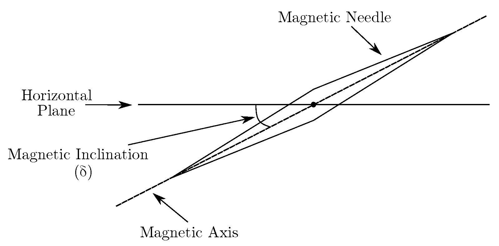
Magnetic inclination is the angle between the horizontal plane and the Earth’s magnetic field lines, as shown in Figure 1. It can be defined by the normalized inner product of the gravity and the magnetic field vectors as

$$sin\delta =\frac{f^{T}m}{\parallel f\parallel \parallel m\parallel },$$

(9)

where $\delta$ is the magnetic inclination angle, f is the gravity vector, and m is the magnetic field vector.

The inclination angle can be calculated using the measurements of a 3-axis accelerometer and a 3-axis magnetometer. For this to be possible however, both sensors must be individually calibrated and their sensitivity axes must be aligned.

Assuming N measurements of a calibrated accelerometer and a calibrated magnetometer, fixed on the same rigid platform, we write the cost function which implicitly captures the misalignment error between the two sensors,

$${\displaystyle J_{al}=\sum _{k=1}^N{\left(sin\delta -\frac{f_k^{T}R{m}_k}{\parallel f_k\parallel \parallel m_k\parallel }\right)}^2.}$$

(10)

Note that $\parallel R{m}_k\parallel =\parallel m_k\parallel$ because $R\in SO\left(3\right)$. Then, we express the axes alignment between the two sensors as the following optimization problem:

$$\begin{array}{cc}\mathrm{minimize}\hfill & J_{al}\hfill \\ \mathrm{subject}\mathrm{to}\hfill & R\in SO\left(3\right)\hfill \\ & \delta \in \left[-\frac{\pi }{2},\frac{\pi }{2}\right],\hfill \end{array}$$

(11)

where $\delta$ is the magnetic inclination angle, $f_k$ and $m_k$ are the accelerometer and magnetometer measurements, respectively, and R is a rotation matrix that rotates the magnetometer’s axes into the accelerometer’s axes. Both inclination angle $\delta$ and rotation matrix R are unknowns.

3.3. Joint Accelerometer’s and Magnetometer’s Calibration with Simultaneous Axes Alignment

Using (7) and (10), we formulate the following cost function:

$${\displaystyle J_{total}={\lambda }_a\sum _{k=1}^N\parallel f_k-H_a{y_a}_k+v_a{\parallel }^2+{\lambda }_m\sum _{k=1}^N\parallel m_k-H_m{y_m}_k+v_m{\parallel }^2+{\lambda }_{al}\sum _{k=1}^N{\left(sin\delta -f_k^{T}R{m}_k\right)}^2.}$$

(12)

The joint calibration and axes alignment of a 3-axis accelerometer and a 3-axis magnetometer is formed as the following optimization problem:

$$\begin{array}{cc}\mathrm{minimize}\hfill & J_{total}\hfill \\ \mathrm{subject}\mathrm{to}\hfill & \parallel f_k\parallel =1,\parallel m_k\parallel =1,k=1,2,\dots ,N\hfill \\ & R\in SO\left(3\right),\delta \in \left[-\frac{\pi }{2},\frac{\pi }{2}\right].\hfill \end{array}$$

(13)

In order to solve (13), we write the corresponding unconstrained cost-plus-penalty function:

$$\begin{array}{cc}\hfill J\left(x\right)& {\displaystyle ={\lambda }_a\sum _{k=1}^N\parallel f_k-H_a{y_a}_k+v_a{\parallel }^2+{\lambda }_{an}{\left(\parallel f_k{\parallel }^2-1\right)}^2}\hfill \\ \hfill & {\displaystyle +{\lambda }_m\sum _{k=1}^N\parallel m_k-H_m{y_m}_k+v_m{\parallel }^2+{\lambda }_{mn}{\left(\parallel m_k{\parallel }^2-1\right)}^2}\hfill \\ \hfill & {\displaystyle +{\lambda }_{al}\sum _{k=1}^N{\left(d-f_k^{T}R{m}_k\right)}^2+{\lambda }_R\left(\parallel R{R}^T{-I\parallel }_F^2+{(detR-1)}^2\right),}\hfill \end{array}$$

(14)

where

$$x={\left[\mathrm{vec}{\left(H_a\right)}^T,{v_a}^T,f_1^T,\dots ,f_N^T,\mathrm{vec}{\left(H_m\right)}^T,{v_m}^T,m_1^T,\dots ,m_N^T,\mathrm{vec}{\left(R\right)}^T,d\right]}^T,$$

${\lambda }_a$, ${\lambda }_{an}$, ${\lambda }_m$, ${\lambda }_{mn}$, ${\lambda }_{al}$, and ${\lambda }_R$ are positive constants and $d=sin\left(\delta \right)$. ${\parallel \circ \parallel }_F$ denotes the Frobenius norm of a matrix [22] and $vec(\circ )$ denotes the vector form of a matrix. Note that the term ${\lambda }_R\left(\parallel R{R}^T{-I\parallel }_F^2+{(detR-1)}^2\right)$ in (14) ensures that the resulting R matrix is in $SO\left(3\right)$, i.e., it is an orthogonal matrix with a determinant equal to one.

The cost-plus-penalty function in (14) is minimized using the gradient descent method. To that purpose, we define $F=\left[f_1,f_2,\dots ,f_N\right]\mathrm{and}M=\left[m_1,m_2,\dots ,m_N\right]$. The gradient of (14) is derived as follows:

$$\nabla J\left(x\right)={\left[{\frac{\partial J\left(x\right)}{\partial vec\left(H_a\right)}}^T,{\frac{\partial J\left(x\right)}{\partial v_a}}^T,{\frac{\partial J\left(x\right)}{\partial F}}^T,{\frac{\partial J\left(x\right)}{\partial vec\left(H_m\right)}}^T,{\frac{\partial J\left(x\right)}{\partial v_m}}^T,{\frac{\partial J\left(x\right)}{\partial M}}^T,{\frac{\partial J\left(x\right)}{\partial vec\left(R\right)}}^T,{\frac{\partial J\left(x\right)}{\partial d}}^T\right]}^T,$$

(15)

where

$$\begin{array}{cc}\hfill \frac{\partial J\left(x\right)}{\partial \mathrm{vec}\left(H_a\right)}& {\displaystyle =2{\lambda }_a\sum _{k=1}^N\left[{y_a}_k\otimes \left(H_a{y_a}_k-f_k-v_a\right)\right],}\hfill \\ \hfill \frac{\partial J\left(x\right)}{\partial v_a}& {\displaystyle =2{\lambda }_a\sum _{k=1}^N\left[-H_a{y_a}_k+v_a+f_k\right],}\hfill \\ \hfill \frac{\partial J\left(x\right)}{\partial f_{\rho }}& =-2{\lambda }_a(H_a{y_a}_{\rho }+f_{\rho }-v_a)+4{\lambda }_{an}{f}_{\rho }{\parallel f_{\rho }\parallel }^2-{\lambda }_{al}{\left[2\left(sin\left(\delta \right)-{f_{\rho }}^{T}R{m}_{\rho }\right){m_{\rho }}^T{R}^T\right]}^T,\hfill \\ \hfill \frac{\partial J\left(x\right)}{\partial \mathrm{vec}\left(H_m\right)}& {\displaystyle =2{\lambda }_m\sum _{k=1}^N\left[{y_m}_k\otimes \left(H_m{y_m}_k-m_k-v_m\right)\right],}\hfill \\ \hfill \frac{\partial J\left(x\right)}{\partial v_m}& {\displaystyle =2{\lambda }_m\sum _{k=1}^N\left[-H_m{y_m}_k+v_m+m_k\right],}\hfill \\ \hfill \frac{\partial J\left(x\right)}{\partial m_{\rho }}& =-2{\lambda }_m(H_m{y_m}_{\rho }+m_{\rho }-v_m)+4{\lambda }_{mn}{m}_{\rho }{\parallel m_{\rho }\parallel }^2-{\lambda }_{al}{\left[2\left(sin\left(\delta \right)-{f_{\rho }}^{T}R{m}_{\rho }\right){f_{\rho }}^{T}R\right]}^T,\hfill \\ \hfill \frac{\partial J\left(x\right)}{\partial vec\left(R\right)}& {\displaystyle =-2{\lambda }_{al}\sum _{k=1}^N\left[\left(sin\left(\delta \right)-{f_k}^{T}R{m}_k\right)\left(m_k\otimes f_k\right)\right]}\hfill \\ \hfill & +4{\lambda }_R\mathrm{vec}\left(R{R}^{T}R-R\right)+2{\lambda }_R(detR-1)\mathrm{vec}\left({\mathrm{adj}\left(R\right)}^T\right),\hfill \\ \hfill \frac{\partial J\left(x\right)}{\partial sin\left(\delta \right)}& {\displaystyle =2{\lambda }_{al}\sum _{k=1}^N\left(sin\left(\delta \right)-{f_k}^{T}R{m}_k\right),}\hfill \end{array}$$

where $\rho =1,2,\dots ,N$ and ⊗ denotes the Kronecker’s product [22].

A good initial estimate of the unknowns is required to ensure the algorithm’s convergence. For the accelerometer, the calibration matrix is initialized as the identity matrix and the offset vector as the zero vector. For the magnetometer, the linear least-squares problem proposed in [11] is used to find an initial estimate of the calibration parameters. The inclination angle is initialized according to the World Magnetic Model (WMM) while the axes alignment matrix R is initialized as the identity matrix.

4. Measurement Platform

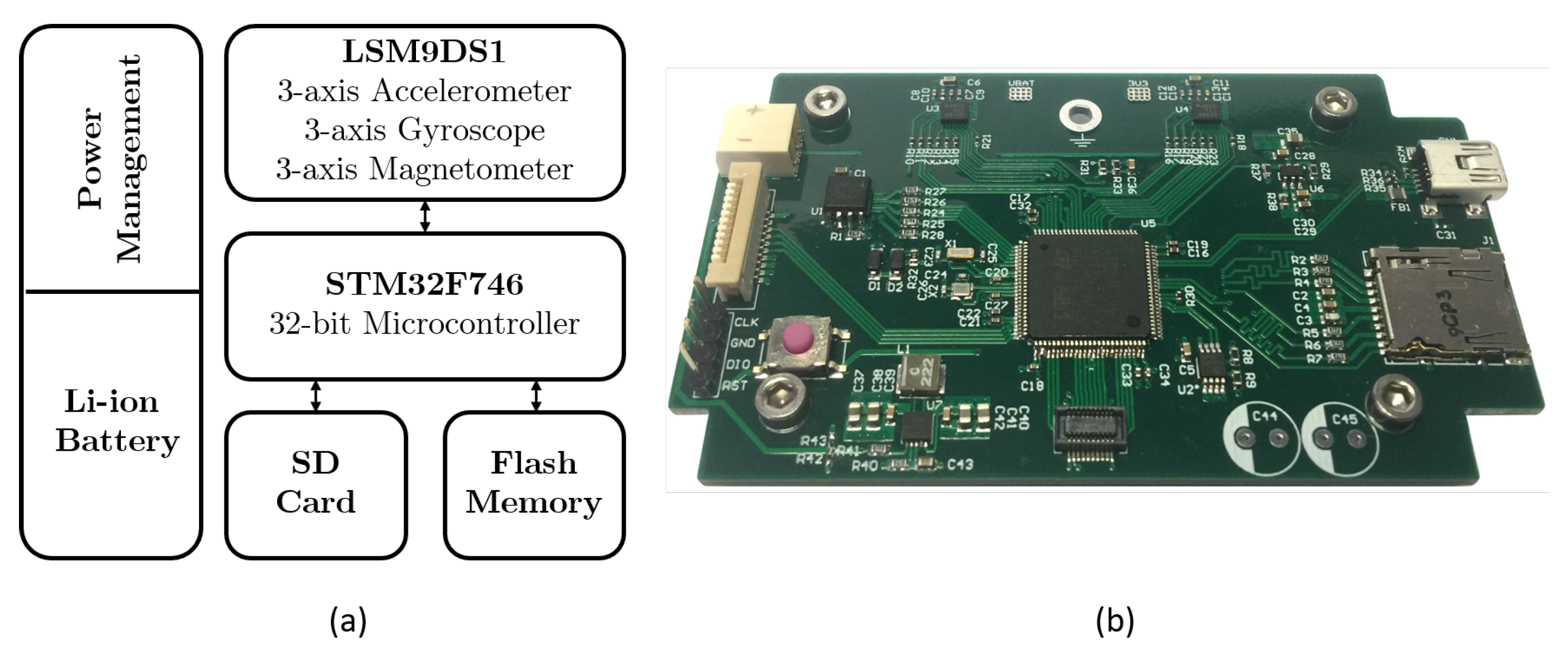
A measurement platform based on low-cost inertial and magnetic sensors was designed and built for experimental purposes. The designed system embeds the STMicroelectronics LSM9DS1 system-in-package (SiP), which contains a 3-axis accelerometer, a 3-axis gyroscope, and a 3-axis magnetometer. The data are handled by a 32-bit microcontroller (STMicroelectronics STM32F746) and stored in flash memory (temporarily) and on an SD card (permanently). The system is powered by a standard $3.7$ V Li-ion battery. A system-level diagram and a picture of the implemented measurement platform are shown in Figure 2.

The basic performance characteristics of the LSM9DS1 SiP are presented in

Table 1. Basic performance characteristics of the LSM9DS1 SiP (Accelerometer).

	Accelerometer
Measurement Range	$\pm 2$ g–$\pm 16$ g
Output Resolution	16 bits
Sensitivity	$0.732$ mg/LSB ($\pm 16$ g )
Output Data Rate (max)	952 Hz

and

Table 2. Basic performance characteristics of the LSM9DS1 SiP (Magnetometer).

	Magnetometer
Measurement Range	$\pm 4$ Gauss–$\pm 16$ Gauss
Output Resolution	16 bits
Sensitivity	$0.58$ mGauss/LSB ($\pm 16$ Gauss )
Output Data Rate (max)	80 Hz

.

Note that during the experimental measurements, the range of the accelerometer and the magnetometer were set to $\pm 16$ g and $\pm 16$ Gauss, respectively. In addition, the accelerometer’s output data rate was set to 238 Hz while the magnetometer’s output data rate was set to 80 Hz.

5. Experimental Results and Algorithm’s Performance

For experimental purposes, we used the measurement platform of Section 4 to record three different calibration datasets. To do so, the measurement platform was placed in 12 different orientations according to the 12-step accelerometer and magnetometer calibration procedure introduced in [8]. The calibration procedure was repeated three times, and three different calibration datasets were recorded. The proposed algorithm was applied to all calibration datasets. Its convergence and accuracy are discussed below.

5.1. Algorithm’s Convergence

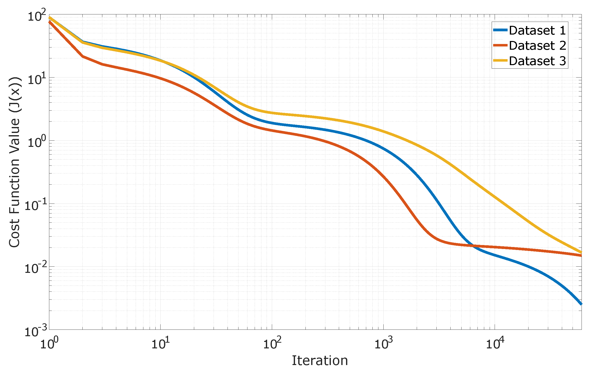
The convergence of the proposed algorithm, evaluated using the cost function $J\left(x\right)$, is shown in Figure 3. The goal of the calibration is to derive a vector x such that $J\left(x\right)$ becomes zero. However, in practical applications, instead of becoming zero, it converges to a very small value. This happens due to the sensor’s nonlinearities and noise, which are not captured by the linear models (2) and (4).

As shown in Figure 3, $J\left(x\right)$ converges to a sufficiently small value for all three datasets in a way that appears to be monotonic. Note that the cost function value evolves differently with the iteration step for every one of the three datasets. This is expected and relates with the calibration procedure used. More specifically, to record each calibration dataset, the measurements platform was placed in 12 different still orientations as recommended in [8]. As the placement of the sensor was done by hand, by three different persons, the orientation deviations (even up to 20 degrees in Euler angle) resulted in different datasets which implied the different evolutions of the cost function value.

5.2. Calibration Parameters

Applying the proposed calibration algorithm to every dataset, we calculated the calibration parameters for the two sensors ($T_a$, $h_a$ and $T_m$, $h_m$ for the accelerometer and the magnetometer, respectively) and the axes alignment matrix R. A brief analysis of the form and numerical values of the calculated parameters is presented below.

The calculated calibration matrix $T_a$ and offset vector $h_a$ for the accelerometer are

$$T_a=\left[\begin{array}{ccc}9.7710& 0.0018& -0.0030\\ 0.0019& 9.7032& -0.0011\\ -0.0087& -0.0013& 9.6927\end{array}\right],h_a=\left[\begin{array}{c}-0.1472\\ -0.0011\\ -0.1274\end{array}\right].$$

The diagonal elements of $T_a$ primarily reflect the necessary scaling of the measurements so that the unit magnitude constraint is fulfilled (note that the sensor’s output is expressed in $m/s^2$). The nondiagonal elements primarily compensate for the cross-coupling error. Their values are quite small as no big axes nonorthogonalities are expected in a typical sensor.

Similarly, the calibration matrix $T_m$ and offset vector $h_m$ are

$$T_m=\left[\begin{array}{ccc}0.4620& -0.0293& -0.0370\\ 0.0686& 0.4379& 0.0303\\ 0.0427& -0.0336& 0.4369\end{array}\right],h_m=\left[\begin{array}{c}-0.1760\\ 0.2214\\ 0.0398\end{array}\right].$$

In the magnetometer’s case, the resulting calibration matrix $T_m$ has a more complicated form as it also incorporates the soft-iron distortion compensation. The values of the diagonal elements of $T_m$ are very close to the required scaling factors for the magnitude normalization (note that the magnitude of the magnetic field at the place of the experiment is about 0.42 Gauss, according to WMM.) and the nondiagonal ones have small absolute values. This indicates that only weak soft-iron distortion is present. In the same vein, the offset vector $h_m$ incorporates both the sensor’s offset and the hard-iron distortion compensation.

Finally, the calculated axes alignment matrix R is

$$R=\left[\begin{array}{ccc}0.9980& -0.0524& -0.0837\\ 0.0592& 0.9936& 0.0597\\ 0.0813& -0.0654& 0.9944\end{array}\right].$$

As expected, R is close to identity matrix. The total axes misalignment between the magnetometer and the accelerometer, expressed in principal rotation parameters, is about ${6.7}^{\circ }$.

5.3. Calibration Accuracy

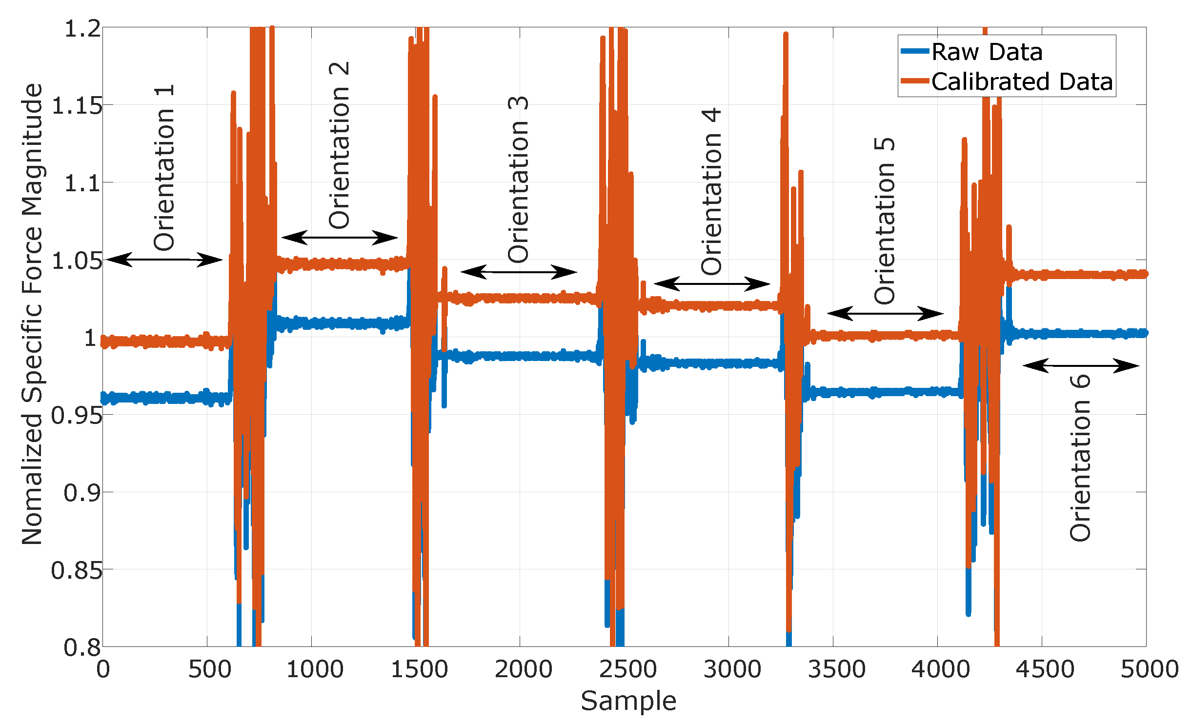
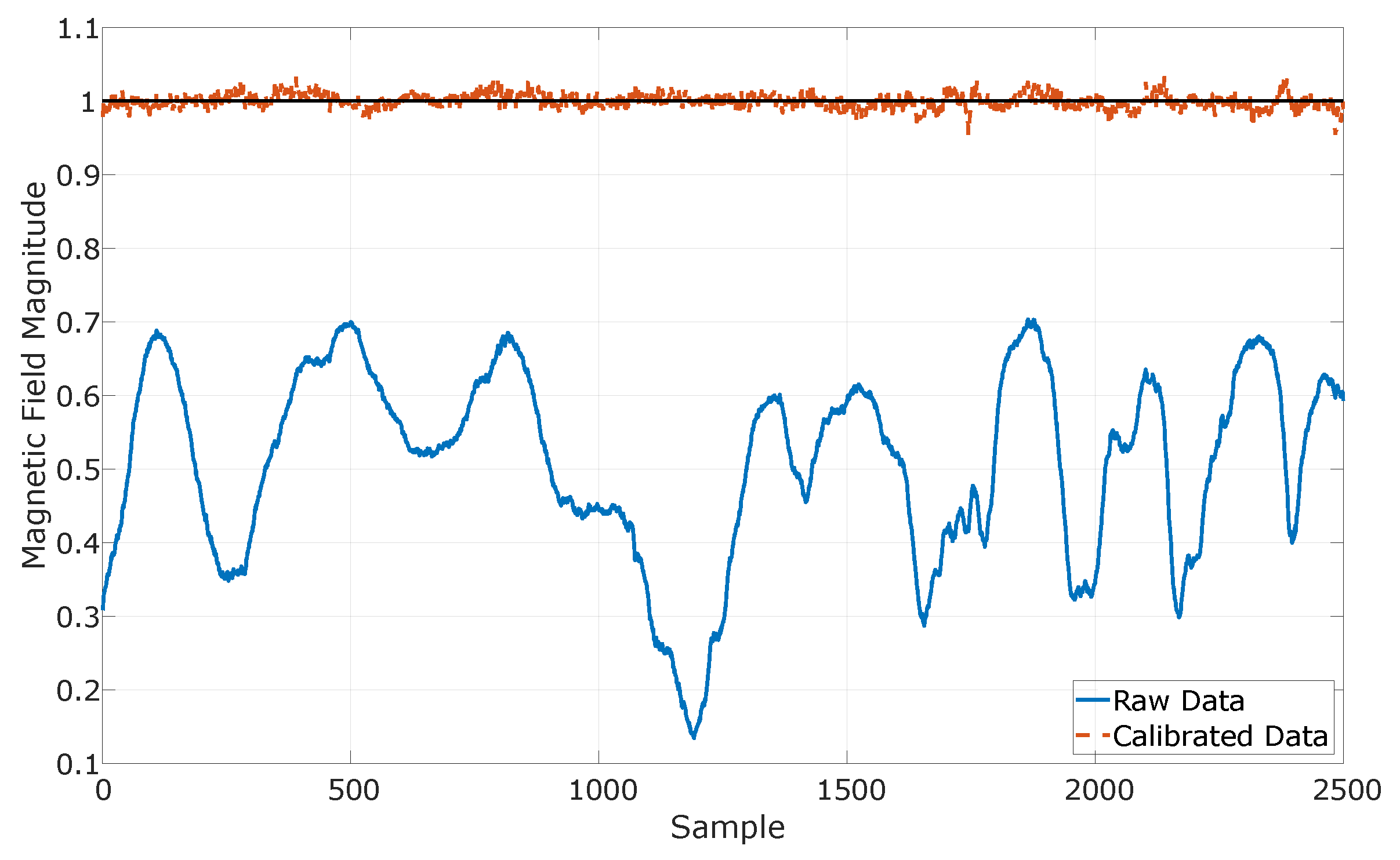
The proposed algorithm exploits the constant magnitude of gravity (for accelerometer’s calibration) and the earth’s magnetic field (for magnetometer’s calibration). Thus, when both sensors are calibrated, the measured magnitude of the specific force and the magnetic field should be constant, independent of the sensor’s orientation. In Figure 4, the accelerometer’s magnitude while the sensor’s platform is placed in several different still positions is presented. Similarly, the magnitude of the raw and calibrated magnetometer’s measurements while the sensors’ platform is randomly rotated by hand is shown in Figure 5.

As seen in Figure 4 and Figure 5, the magnitude of the calibrated measurements is constant and equal to one, independent of the sensor’s orientation, indicating the accurate calibration of both sensors.

As far as the axes alignment is concerned, except from the rotation matrix R, the algorithm also calculates the inclination angle $\delta$. Given that the calibration took place away from any magnetic disturbance (and thus, the measured magnetic field corresponds to the earth’s magnetic field), the measured inclination angle should be close to that predicted by WMM. The inclination angle calculated for each dataset is presented in

Table 3. Inclination angle calculated for each dataset.

Dataset	Inclination Angle ($\mathit{\delta }$)
1	${54.68}^{\circ }$
2	${54.03}^{\circ }$
3	${54.29}^{\circ }$

.

The experimental calibration measurements took place inside the campus of the National Technical University of Athens. According to WMM, the magnetic inclination angle at the location of the experiment is ${54.6025}^{\circ }$. The small deviation of the measured inclination angles from that predicted by WMM indicates the accuracy of the calibration algorithm.

6. Conclusions

In this work, we presented an algorithm for joint calibration and axes alignment of a 3-axis accelerometer and a 3-axis magnetometer. The proposed algorithm applies when the two sensors are fixed on the same rigid platform. It calibrates both sensors and aligns their sensitivity axes without requiring any special piece of equipment or external references. Experimental results demonstrate the algorithm’s convergence and accuracy.

References

- Fischer, C.; Talkad Sukumar, P.; Hazas, M. Tutorial: Implementing a Pedestrian Tracker Using Inertial Sensors. IEEE Pervasive Comput. 2012, 12, 17–27. [Google Scholar] [CrossRef]
- Madgwick, S.O.H.; Harrison, A.J.L.; Vaidyanathan, R. Estimation of IMU and MARG orientation using a gradient descent algorithm. In Proceedings of the 2011 IEEE International Conference on Rehabilitation Robotics, Zurich, Switzerland, 27 June–1 July 2011; pp. 1–7. [Google Scholar] [CrossRef]
- Chu, C. Video stabilization for stereoscopic 3D on 3D mobile devices. In Proceedings of the 2014 IEEE International Conference on Multimedia and Expo (ICME), Chengdu, China, 14–18 July 2014; pp. 1–6. [Google Scholar] [CrossRef]
- Groves, P.D. Principles of GNSS, Inertial, and Multisensor Integrated Navigation Systems. IEEE Aerosp. Electron. Syst. Mag. 2013, 30, 26–27. [Google Scholar]
- Lu, X.; Liu, Z.; He, J. Maximum Likelihood Approach for Low-Cost MEMS Triaxial Accelerometer Calibration. In Proceedings of the 8th International Conference on Intelligent Human-Machine Systems and Cybernetics (IHMSC), Hangzhou, China, 10–11 September 2016; pp. 179–182. [Google Scholar] [CrossRef]
- Ammann, N.; Derksen, A.; Heck, C. A novel magnetometer-accelerometer calibration based on a least squares approach. In Proceedings of the 2015 International Conference on Unmanned Aircraft Systems (ICUAS), Denver, CO, USA, 9–12 June 2015; pp. 577–585. [Google Scholar] [CrossRef]
- Frosio, I.; Pedersini, F.; Borghese, N.A. Autocalibration of MEMS Accelerometers. IEEE Trans. Instrum. Meas. 2008, 58, 2034–2041. [Google Scholar] [CrossRef]
- Papafotis, K.; Sotiriadis, P.P. MAG.I.C.AL.–A Unified Methodology for Magnetic and Inertial Sensors Calibration and Alignment. IEEE Sens. J. 2019, 19, 8241–8251. [Google Scholar] [CrossRef]
- Glueck, M.; Buhmann, A.; Manoli, Y. Autocalibration of MEMS accelerometers. In Proceedings of the 2012 IEEE International Instrumentation and Measurement Technology Conference Proceedings, Graz, Austria, 13–16 May 2012; pp. 1788–1793. [Google Scholar] [CrossRef]
- Alonso, R.; Shuster, M.D. TWOSTEP: A fast robust algorithm for attitude-independent magnetometer-bias determination. J. Astronaut. Sci. 2002, 50, 433–451. [Google Scholar]
- Wu, Y.; Shi, W. On Calibration of Three-Axis Magnetometer. IEEE Sens. J. 2015, 15, 6424–6431. [Google Scholar] [CrossRef] [Green Version]
- Kok, M.; Schön, T.B. Maximum likelihood calibration of a magnetometer using inertial sensors. IFAC Proc. Vol. 2014, 47, 92–97. [Google Scholar] [CrossRef] [Green Version]
- Kok, M.; Schon, T.B. Magnetometer Calibration Using Inertial Sensors. IEEE Sens. J. 2016, 16, 5679–5689. [Google Scholar] [CrossRef] [Green Version]
- Vasconcelos, J.F.; Elkaim, G.; Silvestre, C.; Oliveira, P.; Cardeira, B. Geometric Approach to Strapdown Magnetometer Calibration in Sensor Frame. IEEE Trans. Aerosp. Electron. Syst. 2011, 47, 1293–1306. [Google Scholar] [CrossRef] [Green Version]
- Wu, Y.; Zou, D.; Liu, P.; Yu, W. Dynamic Magnetometer Calibration and Alignment to Inertial Sensors by Kalman Filtering. IEEE Trans. Control Syst. Technol. 2018, 26, 716–723. [Google Scholar] [CrossRef] [Green Version]
- Wu, Y.; Luo, S. On Misalignment Between Magnetometer and Inertial Sensors. IEEE Sens. J. 2016, 16, 6288–6297. [Google Scholar] [CrossRef]
- Kok, M.; Hol, J.D.; Schön, T.B.; Gustafsson, F.; Luinge, H. Calibration of a magnetometer in combination with inertial sensors. In Proceedings of the 15th International Conference on Information Fusion, Singapore, 9–12 July 2012; pp. 787–793. [Google Scholar]
- Gheorghe, M.V. Calibration for tilt-compensated electronic compasses with alignment between the magnetometer and accelerometer sensor reference frames. In Proceedings of the 2017 IEEE International Instrumentation and Measurement Technology Conference (I2MTC), Turin, Italy, 22–25 May 2017; pp. 1–6. [Google Scholar] [CrossRef]
- Noureldin, A.; Karamat, T.B.; Georgy, J. Fundamentals of Inertial Navigation, Satellite-based Positioning and their Integration; Springer: Berlin/Heidelberg, Germany, 2013. [Google Scholar]
- Metge, J.; Mégret, R.; Giremus, A.; Berthoumieu, Y.; Décamps, T. Calibration of an inertial-magnetic measurement unit without external equipment, in the presence of dynamic magnetic disturbances. Meas. Sci. Technol. 2014, 25, 125106. [Google Scholar] [CrossRef]
- Papafotis, K.; Sotiriadis, P.P. Computationally Efficient Calibration Algorithm for Three-Axis Accelerometer and Magnetometer. In Proceedings of the 8th International Conference on Modern Circuits and Systems Technologies (MOCAST), Thessaloniki, Greece, 13–15 May 2019; pp. 1–4. [Google Scholar] [CrossRef]
- Horn, R.A.; Johnson, C.R. Matrix Analysis; Cambridge University Press: Cambridge, UK, 2013. [Google Scholar]
Figure 1.
Magnetic inclination.
Figure 2.
System-level diagram (a) and picture (b) of the implemented measurement platform.
Figure 3.
Algorithm’s convergence for three different datasets.
Figure 4.
Normalized magnitude of raw and calibrated accelerometer’s data while the sensor is placed in different still positions.
Figure 5.
Magnitude of raw and calibrated magnetometer’s measurements while the sensor is randomly rotated by hand.