
The Dynamic Spillover Effects of Macroeconomic and Financial Uncertainty on Commodity Markets Uncertainties


1
Department of Finance and Investment, College of Economics and Administrative Sciences, Imam Mohammad Ibn Saud Islamic University, Riyadh 13318, Saudi Arabia
2
Department of Economics and Quantitative Methods, University of Sfax, Sfax 3029, Tunisia
3
Department of Economics, University of Gabes, Gabes 6029, Tunisia
*
Author to whom correspondence should be addressed.
Economies 2021, 9(2), 91; https://0-doi-org.brum.beds.ac.uk/10.3390/economies9020091
Submission received: 3 May 2021
/
Revised: 5 June 2021
/
Accepted: 7 June 2021
/
Published: 15 June 2021
Abstract
:The present paper has two main objectives: first, to accurately estimate commodity price uncertainty; and second to analyze the uncertainty connectedness among commodity markets and the macroeconomic uncertainty, using the time-varying vector-autoregressive (TVP-VAR) model. We use eight main commodity markets, namely energy, fats and oils, beverages, grains, other foods, raw materials, industrial meals, and precious metals. The sample covers the period from January 1960 to June 2020. The estimated commodity price uncertainties are proven to be leading indicators of uncertainty rather than volatility in commodity markets. In addition, the time-varying connectedness analysis indicates that the macroeconomic uncertainty has persistent spillover effects on the commodity uncertainty, especially during the recent COVID-19 pandemic period. It has also found that the energy uncertainty shocks are the main drivers of connectedness among commodity markets, and that fats and oils uncertainty is the influence driver of uncertainty spillovers among agriculture commodities. The achieved results are of important significance to policymakers, firms, and investors to build accurate forecasts of commodity price uncertainties.
1. Introduction
Much attention has been devoted to commodity price movements since the early 2000s. The rapid growth of investments in commodities and excessive commodity price volatility during the last two decades makes it clear that commodity price fluctuations are of great importance for investors, policymakers, and researchers. Recently, several studies argued that uncertainty shocks are important sources of commodity price volatility (Van Robays 2016; Joëts et al. 2017; Bakas and Triantafyllou 2018, 2020; Watugala 2019; Naeem et al. 2021). However, there are few studies that estimate commodity price uncertainty and the dynamic spillovers of macroeconomic uncertainty on commodity price uncertainty. The present paper seeks to contribute in this respect.
The 2007–2009 global financial crisis has raised the question of whether economic and financial uncertainty may explain the unpredictable components of commodity prices. An extensive literature has examined the influence of economic and financial variables on commodity prices and their potential to forecast commodity price movements (e.g., Ye et al. 2006; Coppola 2008; Chen et al. 2010; Alquist and Kilian 2010; Groen and Pesenti 2011; Hong and Yogo 2012; Baumeister and Kilian 2012, 2015; Bessembinder and Chan 2016; Ahumada and Cornejo 2016; Wang et al. 2017; Baumeister et al. 2018). Other studies explore the role of economic uncertainty in explaining commodity price returns and volatility (e.g., Yin and Han 2014; Bakas and Triantafyllou 2018, 2019; Joëts et al. 2017; Bahloul et al. 2018; Yang 2019).
The main objective of this paper is to accurately estimate commodity price uncertainty and to explore afterwards the spillover effects of macroeconomic uncertainty on commodity price uncertainty. To do this, we use a monthly dataset that contains 8 main commodity groups, including energy, beverages, fats and oils, grains, other food, raw materials, industrial metals, and precious metals. First, we use the macroeconomic uncertainty (MU, thereafter) measure proposed by Jurado et al. (2015) Authors use comprehensive macroeconomic (132 macro series) and financial (147 financial series) datasets and construct a monthly-based macroeconomic uncertainty measure for the period 1960:7–2011:12. The measure is updated, now covering 1960:7–2020:6. The MU measure is defined as the aggregate of the individual conditional variance of the unpredictable part of each of a set of macroeconomic variables. Then, we apply the econometric methodology proposed by Jurado et al. (2015) to estimate the commodity price uncertainty. Finally, we estimate and analyze the uncertainty spillover effects between commodity uncertainties and MU measure.
The rationale behind the use of commodity price uncertainty instead of commodity price volatility is that uncertainty measures the unexpected variation of commodity price, while volatility is the expected variation of commodity price (Balli et al. 2019). Besides, Jurado et al. (2015) find that their estimated macroeconomic uncertainty measure explains accurately the observed fluctuations in real activity.
This study contributes to the related literature on commodity connectedness in two ways. First, we estimate the monthly price uncertainty of eight broad commodity markets employing the econometric approach proposed by Jurado et al. (2015). The advantage of this approach is to assign uncertainty to unpredictable shocks. Second, we examine the dynamic connectedness between commodity markets uncertainty and the macroeconomic uncertainty. The purpose is to examine the time-varying linkages between economic and financial uncertainty and commodity prices uncertainty. Thus, we use an extension of the usual Diebold and Yilmaz (2014) connectedness approach to the time-varying parameters autoregressive (TVP-VAR) setting (Korobilis and Yilmaz 2018; Antonakakis et al. 2020).
Our results reveal, on one hand, that the different estimated commodity price uncertainties can track episodes of heightened macroeconomic and financial uncertainty, mainly the 2001 and 2007–2009 crises periods. On the other hand, the estimated commodity price uncertainty measures provide evidence that these measures are forward-looking indicators and can predict commodity price uncertainty in advance. Finally, the dynamic connectedness results provide ample evidence of significant inter-market connectedness across commodity markets and economic and financial uncertainty, especially during the 2007–2009 global financial and European debt crises and the recent COVID-19 pandemic crisis.
2. Literature Review
Recently, the periods of uncertainty on economic and political events are argued to be responsible of great fluctuations in commodity prices. Broadly, there are two strands of the literature that examine the nexus between macroeconomic variables and commodity prices fluctuations. The first strand investigates the returns and volatility spillovers among commodity prices. Silvennoinen and Thorp (2013) find that most correlations between commodity markets start weakly beginning in the 1990s, but closer integration emerges around the early 2000s and reaches a peak during the recent crisis. Arouri et al. (2011b) use a bivariate GARCH model to estimate the volatility spillover effect between the stock market and commodity market (oil market) in Europe and the U.S for the period from 1998 to 2008. They find a spillover effect between commodity market to stock market for the case of Europe, while a bidirectional spillover effects was found for the U.S. Similarly, Arouri et al. (2011a) examine the effect of volatility spillovers among stock market and commodity market (oil market) in the GCC countries. They found strong evidence of volatility spillovers effect between GCC countries. Moreover, Du et al. (2011) find evidence of a volatility spillover between some agricultural commodity prices and energy prices. Mensi et al. (2013) examine the joint evolution of conditional returns, the correlation and volatility spillovers between the markets for beverages, agricultural commodities, crude oil, metal, and stock exchange over the turbulent decade 2000–2011. The results show a significant correlation and volatility transmission between commodity and equity markets. Barbaglia et al. (2020) explore the volatility spillovers between some energy, agricultural, and biofuel commodities by using the VAR model. They find evidence of volatility spillovers between energy and agricultural commodities.
The second one examines the impact of uncertainty shocks on commodity prices returns and volatility. Unlike used volatility indicators, the uncertainty shock measure is depicted as the conditional volatility of the unpredictable component of a few commodity prices as presented by Jurado et al. (2015). Yin and Han (2014) find that heightened uncertainty concerning macroeconomic volatility is the source of the observed high prices and volatility in commodity markets. Van Robays (2016) uses a structural threshold VAR model to examine the impact of macroeconomic uncertainty on oil shocks. He estimates the effects of oil supply and demand shocks under low and high regimes of uncertainty. He finds that oil supply and demand shocks have significant effects on economic activity under high uncertainty regimes. Bekiros et al. (2015) show that information on economic policy uncertainty helps to forecast oil price returns accurately. Wang et al. (2015) and provide evidence that economic policy uncertainty is the best predictor of oil price volatility. Badshah et al. (2019) find a significant positive effect of EPU on stock-commodity correlations with particularly strong effects in the case of energy and industrial metals. Similarly, Zhu et al. (2020) investigate the asymmetric effect of EPU on China’s agriculture and metal futures returns using the panel quantile regression approach. They conclude that the domestic EPU shocks have a significant negative effect on agricultural futures returns in bearish markets and a significant positive effect on metal futures returns in bullish markets.
Using some observable and unobservable measures of macroeconomic uncertainty, Bakas and Triantafyllou (2018, 2019) show the important role of latent macroeconomic uncertainty in explaining commodity price volatility. The authors find that the latent (unobservable) uncertainty measure of Jurado et al. (2015) has a more significant impact on the volatility of commodity prices than the observable economic uncertainty (such as the VOX or the EPU). Moreover, they provide evidence that the JLN macroeconomic uncertainty measure can better forecast the volatility of energy, metals, and agricultural commodity futures returns and make commodity markets less volatile.
Joëts et al. (2017) use a structural threshold vector autoregressive (TVAR) model on a sample of 19 commodity markets to examine the impact of macroeconomic uncertainty on oil and commodity price volatility. They demonstrate that commodity price markets are overly sensitive to macroeconomic uncertainty shocks. Furthermore, Bahloul et al. (2018) provide evidence that economic and financial uncertainties can predict movements in commodity futures markets. The results of Bakas and Triantafyllou (2020) show that during the recent COVID pandemic period, the increase in pandemic uncertainty reduces volatility in commodity markets. In particular, the pandemic uncertainty has a negative impact on oil markets and a less significant positive effect on gold markets.
Using a structural VAR model, Kang and Ratti (2013) examine in their pioneering work the causal impacts of oil price shocks and economic policy uncertainty. They find spillover effects between oil price shocks and economic policy uncertainty, and jointly affect the stock markets. In the same line, Antonakakis et al. (2014) and Chen et al. (2010) note that oil price shocks and economic policy uncertainty influence each other negatively. Furthermore, Diebold et al. (2017) study the static and dynamic connectedness between 19 commodity markets (energy, grains, softs, industrial metals, livestock, and precious metal commodities). Their results reveal that energy is the most net transmitter of shocks to others, and energy, industrial metals and precious metal are themselves tightly connected. Yang (2019) shows evidence of strong connectedness between oil shocks and global economic uncertainty, and the latter is net transmitter of shocks to oil market.
Balli et al. (2019) estimate a time varying uncertainty index for 22 commodities, and they investigate the connectedness between these commodities by using the connectedness model of Diebold and Yilmaz (2014). Their results show an increase in connectedness among commodity uncertainty indexes during the global financial crisis and the oil price collapse of 2014–2016. Naeem et al. (2021) use the Diebold and Yilmaz approach based on forecast error variance decomposition to investigate the spillover of uncertainty among 17 commodities during the period 2007–2016. The results suggest that oil is the most transmitter of uncertainties to other commodity markets, and this transmission increases during the turmoil periods. Additionally, they find that the global factors have a significant effect on the connectedness among oil and other commodity uncertainties.
Therefore, unlike previous studies, which examine the impacts of uncertainty shocks on the volatility of commodity prices and the volatility spillovers in commodity markets, our study seeks to investigate the influence of global factors (such as macroeconomic and financial uncertainty or the economic policy uncertainty) in driving the spillover uncertainty between commodity markets.
3. Data and Preliminary Analysis
We consider a dataset of eight groups of monthly commodity prices, namely energy (ENRG), beverages (BVG), fats/oils (Foils), grains (GRN), other foods (OTF), raw materials (RWM), industrial metals (MTL), and precious metals (MTL). The time span is the period from January 1960 to June 2020. In addition, we include one-month ahead macroeconomic uncertainty (MU) measure proposed by Jurado et al. (2015). Table A1 in Appendix A details the description, transformation, and the sources of spot commodity prices and MU measure. Figure 1 displays the estimated MU of Jurado et al. (2015).
Table 1 reports the descriptive and integration properties of the commodity price returns. The results indicate that returns on raw materials commodity prices are the smallest volatile market, while returns on energy commodity prices are the most volatile market. All commodity price returns are negatively skewed time series and exhibit high values of Kurtosis, indicating the presence of sharp peaks in these markets. The Jarque–Bera (J–B) statistics reject the null hypothesis of normal distribution. The unconditional correlations matrix shows significant positive correlations among commodity price returns. Furthermore, the Ljung–Box Q–test statistics (at lag 20, Q[20]) support the hypothesis of autocorrelation for the commodity price returns. In addition, the standard ERS unit root test and Z-A break unit root test suggest that commodity price returns behave like stationary processes. The unconditional correlations reveal that all commodity price returns are positively correlated with each other. Moreover, the highest unconditional correlation is observed between the grains and fats and oils markets. The results are in line with many other studies (e.g., Bahloul et al. 2018; Joëts et al. 2017; Diebold et al. 2017; Bakas and Triantafyllou 2018, 2020).
4. Econometric Methodology
The econometric methodology involves two steps. First, we employ the approach of Jurado et al. (2015) to construct the uncertainty measure of each commodity market. Second, we examine the directional (net) return spillovers across commodity price uncertainties and the macroeconomic uncertainty.
4.1. Measuring Commodity Price Uncertainty
To construct the commodity price uncertainty, we apply the Jurado et al. (2015) approach, which consists in:
- Extracting the common factors among 8 commodity price returns. The statistic principal component analysis is used to estimate the common factors.
- Estimating the following factor augmented vector autoregression (FAVAR) model:where , is the commodity price returns of market , and is a vector of the estimated common factors , and a The set of predictors include the squares of the estimated common factors and common factors in to account for possible nonlinearity.
- Computing the ahead prediction error of , and each factor in and . These ahead prediction errors are assumed to have time-varying volatilities. The time-varying squared forecast error is computed using a stochastic volatility model. Jurado et al. (2015) use the STOCHVOL package in R to estimate the volatilities in AR(1) model with stochastic volatility. Then, the ahead commodity price uncertainty of market denoted by is computed as the conditional volatility of the purely unforecastable component of the future value of the series.
4.2. Measuring Commodity Price Uncertainty
The dynamic connectedness approach introduced by Diebold and Yilmaz (2014) is based on the rolling-window based VAR model. Recently, studies, including Antonakakis et al. (2020) and Korobilis and Yilmaz (2018), combine the usual DY connectedness approach with the time-varying parameter VAR (TVP-VAR) methodology. This approach has the advantage of overcoming the arbitrary choice of the rolling-window size, and the sensitivity of the estimated spillover index to outliers (Antonakakis et al. 2020). Accordingly, we use the following TVP-VAR specification to analyze the dynamic connectedness across commodity markets and the MU:
where and the vector of commodity uncertainty, is vector, is is dimensional matrix, and is the matrix of dimension . The error terms and are the matrices of dimension and , respectively. The time-varying variance-covariance and are the matrices of dimension and , respectively. The time-varying covariances matrix follow the exponentially weighted moving average (EWMA) model that depends on decay factor , while the time-varying covariance matrices depends on the forgetting factor .
The construction of the generalized connectedness procedure of Diebold and Yilmaz (2014) is based on the transformation of the TVP-VAR to vector moving average (VMA) representation (Wold representation) and the generalized variance decomposition introduced by Koop et al. (1996) and Pesaran and Shin (1998). Accordingly, the h-step forecast error variance decomposition is defined as:
where is the standard deviation of the error term, and is the selection vector with one in its ith element and zero elsewhere. To solve the problem that , each element of the variance decomposition matrix can be normalized by its row sum:
where , and . The total connectedness index is, therefore, defined as:
The directional connectedness from market to all other markets is given by:
Similarly, the directional connectedness from all other markets to market is given by:
The two directional connectedness provides information on the magnitude of transmission channels of intra-and inter-regional spillovers across markets. Then, it is possible to investigate if a market is a net transmitter or net receiver of shocks by computing the net connectedness index:
Moreover, the net pairwise spillover between markets and is defined as the difference between the gross shocks transmitted from market to market and vice versa. Therefore, the net pairwise total directional connectedness is given by:
5. Empirical Results
5.1. Estimates of Commodity Price Returns Uncertainty
Following Jurado et al. (2015), we use the information criteria proposed in Bai and Ng (2002) to select the number of common factors. The information criteria suggest forecasting factors. The number of lags in the FAVAR model is according to Akaike information criteria.
Table 2 provides the descriptive statistics of the commodity and macroeconomic uncertainties estimates at horizon . The higher uncertainty is observed in the raw materials market, the smaller volatility is energy uncertainty. Furthermore, the Ljung–Box Q–test statistics (at lag 20, Q[20]) support the hypothesis of autocorrelation for the commodity uncertainties.
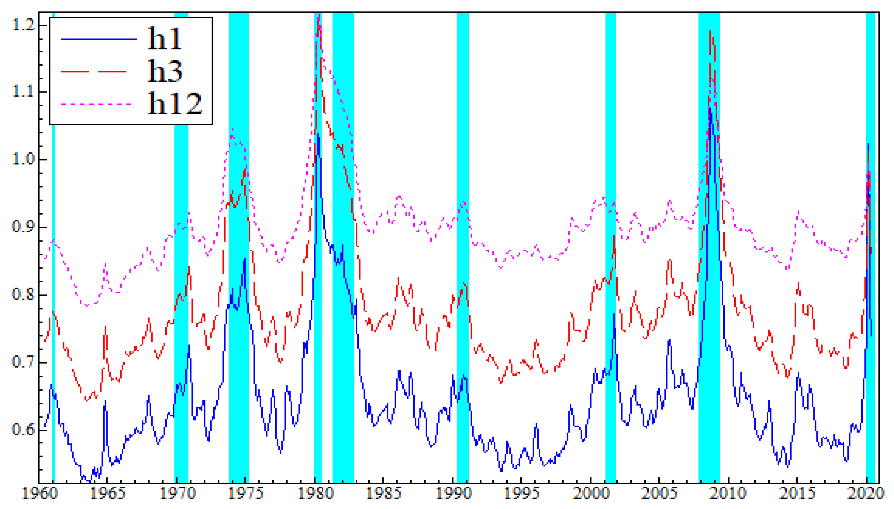
Figure 2 plots the behavior of price uncertainty in energy sector for different horizons. The energy uncertainty index shows that, whatever the time horizons, episodes with heightened price uncertainty in energy sector coincide with the NBER recession period. Precisely, we observe that the higher price uncertainty is more pronounced during the first oil crisis erupted in October 1973. During this period, the rising oil prices leaded to rapid rise in inflation that directly affected both consumers and investors and increase uncertainty in energy market. In addition, we observe that uncertainty in the energy market was reinforced by the 1990 oil price shock, occurring in response to the first gulf war 1990–1991 (the 1990 Iraqi Invasion of Kuwait). Furthermore, our index detects a spike during the 2007–2009 global financial crisis, which implies that shocks, occurring in energy markets, leading to the oil price surge during the 2007–2009 global financial crisis, have generated higher price uncertainty. The relevance of our uncertainty index is reinforced by the prediction of the recent trend occurred in response with the health crisis of COVID-19 pandemic, which started in December 2019. This crisis generates a higher price uncertainty in energy market because of the safety measures adopted by authorities to limit the spread of this virus. These safety measures (the quarantine, travel restriction etc.) affect at the same time the supply and demand of oil and worsen stability in energy market.
Considering the good safe-haven during periods of economic and political uncertainty, precious metals price fluctuations (mainly for the gold) reflect the investor’s behavior who flock to gold in crisis period to protect their assets (Hergt 2013). As shown in Figure 3, the precious metal uncertainty index predicts four periods of price uncertainty in precious metal market. Only three episodes of uncertainty coincide with the NBER crisis period. The first period of uncertainty appears in the beginning of 1975, two years after the first petroleum shock of 1973, which indicates that uncertainty in the precious metals market appears in the long run because the safe haven role of precious metal moves the short-run uncertainty to a longer one (Joëts et al. 2017).
The second period coincides with the highest price uncertainty of precious metals. It has occurred during the three first months of 1980. This period coincides with some events that led to dramatic fall in gold price: the Russian invasion of Afghanistan in December 1979 and the Iranian revolution that caused a second oil crisis. These events are the main cause of the gold price surge in 1980. The rapid growth of oil prices and the economic recession led to a third episode of uncertainty (1981–1982) following the start of the first gulf war between Iraq and Iran creating panic and a run-on gold that forced investors to increasingly buy gold as risk insurance. Hence, precious metal turn into a safe haven in times of uncertainty. In addition, our findings prove that the uncertainty index predict a fourth uncertainty episode of uncertainty just before the global financial crisis of 2007–2009, which illustrates demonstrates the forward character of our uncertainty index.
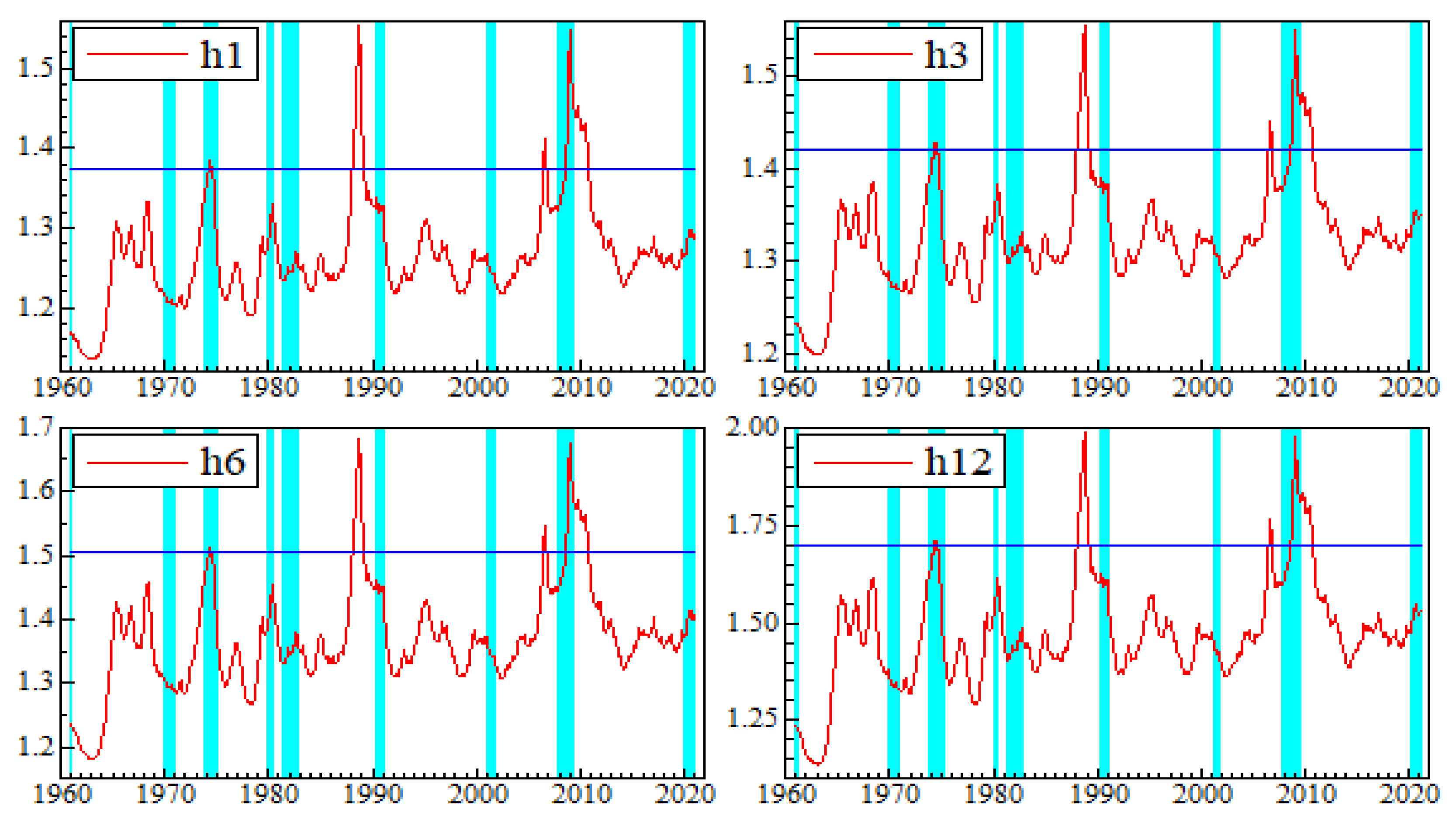
Figure 4 displays the estimates of the industrial metal’s uncertainty index. This figure shows that the uncertainty index predicts four uncertainty episodes. Only two episodes coincide with the NBER recessions. The two other periods of uncertainty reinforce the forward character of our uncertainty index. The first episode was generated during the 1973–1975 recession, which followed the first petroleum shock of October 1973. During this period, the heightened uncertainty in the metal market was mainly due to the steel crisis in the United States and the European countries, which led to the collapse of steel prices because of the decline of demand. The heightened uncertainty episode was predicted by the index earlier before the first gulf war. The third episode had predicted in the beginning of 2007 global financial crisis.
The fourth episode of uncertainty coincides with global financial crisis period (2007–2009). The higher price uncertainty in metals and minerals markets during the 2007–2009 period can be explained by the strong link between metals and mining sector and global economic activity. In this way, metals and mining commodities are considered important for human wellbeing and fundamental for virtually all sectors of the economy (Gankhuyag and Gregoire 2018). Price uncertainty in metals and minerals markets is mainly due to the crisis experienced by the aluminum industry. More precisely, the unexpected strong demand growth of aluminum made by China during the global financial crisis boosted uncertainty. Due to the fast-growing of China aluminum industry, China’s share of global aluminum demand increased from 14 percent in 2000 to 42 percent in 2011 (World Bureau of Metal Statistics, https://www.world-bureau.com/, (acceded on 12 January 2021). Similarly, Stuermer (2018) shows that the strong demand shocks from 2005 to 2007 is mainly due to the rapid industrialization in some countries such as China, which causes fluctuations of mineral commodity prices.
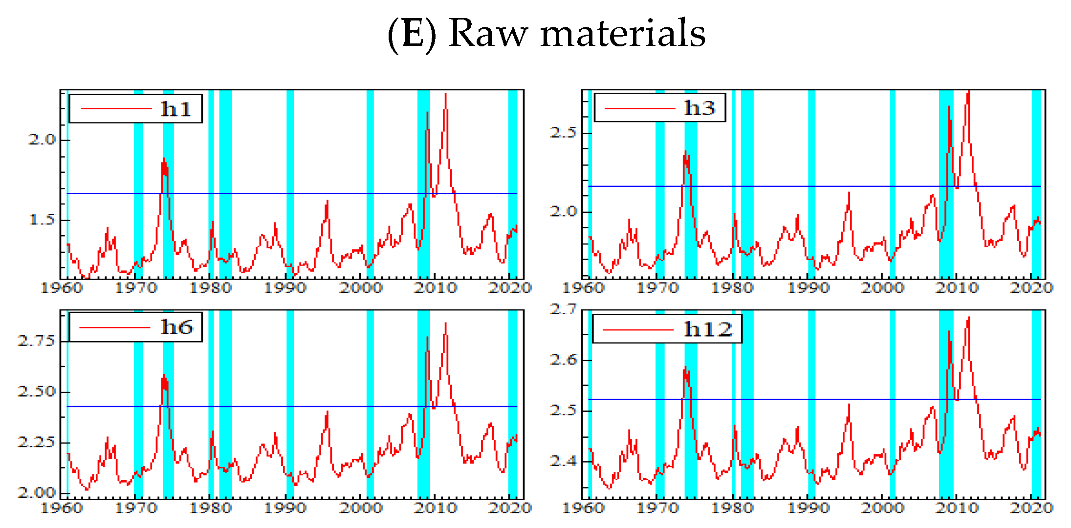
Figure 5 reports the various agriculture commodities uncertainties. The indices predict three uncertainty episodes. The first episode coincides with the first oil shock of 1973. During this period, the higher energy prices raised the cost of production. Indeed, assuming that the agriculture sector is energy-intensive, an increase in the price of oil was followed by higher input costs, lower production, higher prices, and an uncertain effect on net farm income (). Assuming the strong relationship between the energy prices and the agriculture commodity prices (Shiferaw 2019), the increases in energy prices hurt the agricultural sector leading to a food price surge and more uncertainty.
The second episode of higher price uncertainty concerns the 2007–2009 global financial crisis. As mentioned by Wiggins et al. (2010), the spiking energy price is a key determinant of the food price surge during 2007–2008. The U.S great recession has created a higher instability in food prices, which have dramatically increased since 2007. In 2008, food prices increased by around 6.4% in 2008 (Kuhns and Okrent 2019). Considered as the strongest since the 1980s, this spike is followed by a third uncertainty episode during 2010–2011, as detected by the agriculture index. After the world food crisis following the 2007–2009 global financial crisis, food prices around the world again started to rise in 2010, which induces a political and economic uncertainty in agricultural commodities markets.
5.2. Connectedness between Macroeconomic Uncertainty and Commodity Market Uncertainty
We estimate a TVP-VAR with lag 1 accordingly to Akaike information criterion, and the decay and forgotten factors are set to 0.99 and 0.96, respectively. The connectedness uncertainty indices are computed based on 20-month forecasts.
5.2.1. Total Connectedness among Commodities and Macroeconomic Uncertainty Indexes
Diebold et al. (2017) consider that connectedness is important in terms of determining risk measurement and management in the context of commodities. They find that commodity price uncertainty tends to generate higher connectedness. Table 2 shows the averaged dynamic connectedness measures. The static TCI is equal to 61.5%, indicating that the commodity uncertainties are highly interconnected. Moreover, the results suggest that the energy uncertainty is the main driver of connectedness across commodities since it is the net transmitter to all three other commodities and macroeconomic uncertainty followed by the fats and oils, and to a lesser extent the precious metals. On the other hand, the main net receiver is the Other Foods market, which receives from all others, followed by the industrial metals.
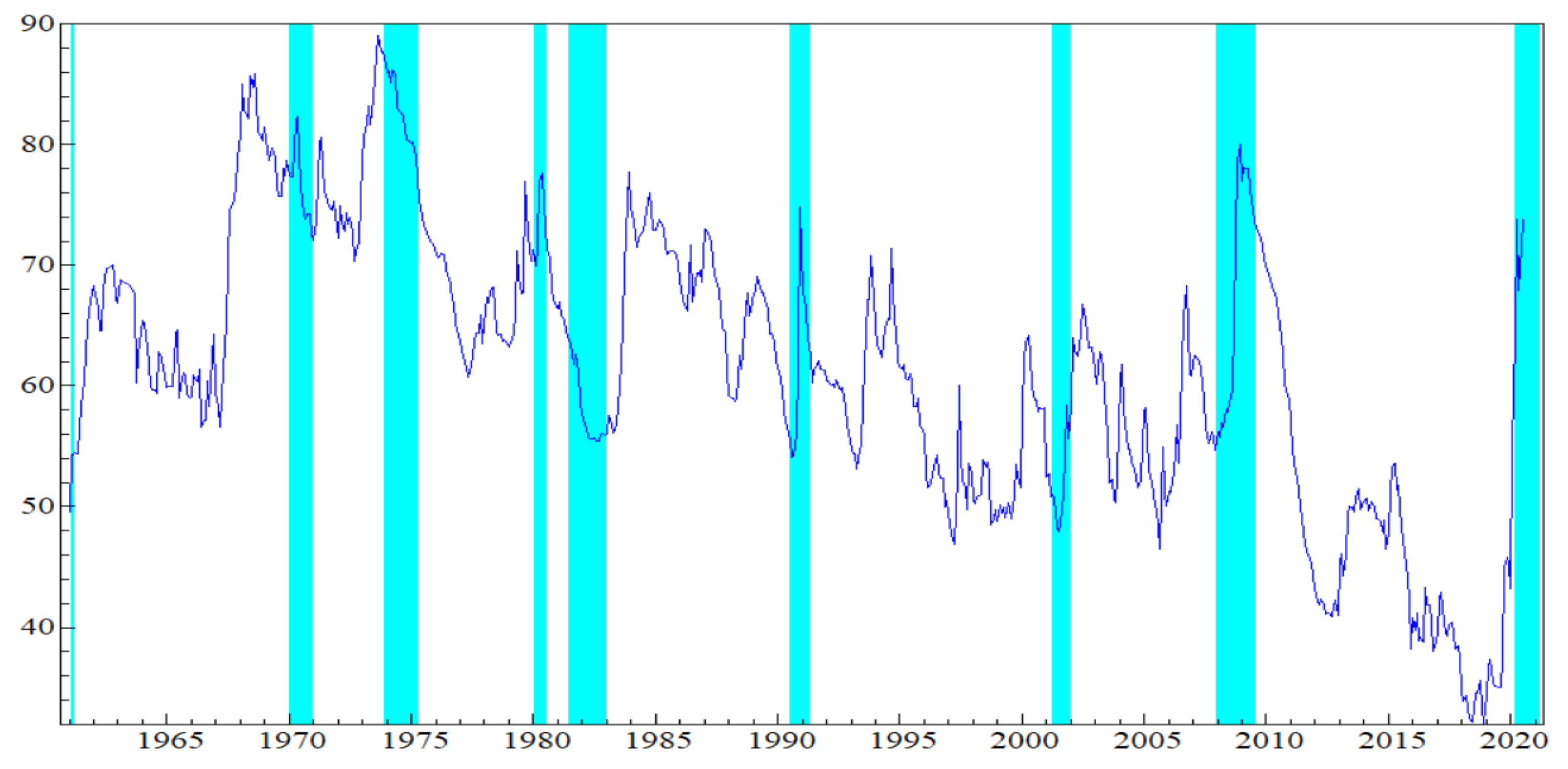
Figure 6 shows total system-wide connectedness among commodity prices and macroeconomic uncertainty. We can see a high total spillover that reached 61.46% over the sample period from December of 1960 to June 2020. Usually during crises periods, commodities prices swing downward due to increased uncertainty, and this in turn leads the system of commodity connectedness to turn upward. From this graph, we can see that total connectedness reaches many peaks that coincide with different turbulent events occurring throughout recent decades. However, the magnitude of the connectedness exceeds 50% from the beginning of the sample until 2011, followed by a drop below 50% until 2020 and a recovery of total spillovers magnitude just after the triggering of Coronavirus pandemic. In the beginning, we can see a spike that reached 85% at the end of 1960s due to an increase in the net uncertainty spillovers of the precious metals as presented in Figure 7. Then during the period 1970–2000s, many spikes reaching high magnitude are observed in total connectedness caused by an increase in uncertainty spillovers of energy that occurred from several events, such as the first oil crisis in the 1970s, the second oil crisis and the recession in 1980s, the Iraq war in 1991 and 2003, and also by an increase in uncertainty spillovers of fats and oils and beverages during the 1990s and 2000s following the increasing financialization and greater synchronization among raw materials (Poncela et al. 2014).
In fact, Krugman (2008) examines the channels of transmission between commodity prices and finds that the increase in energy prices may affect upward the production cost, which impacts the final price of other commodities. Also, the increase in the biofuel demand may reduce the food supply intended to household consumption and increase its prices. During the Great Financial crisis of 2007–2009, another peak reaching 80% is observed due to an increase in uncertainty spillovers of metals, grains, and fats oils. In that period, the systemic risks were very high and the uncertainty about the future prices of commodities increased. This result is in line with the finding of Kang et al. (2017), which reveals a higher spillover among commodities during the global financial crisis. After significant positive actions taken by the developed countries, a sharp decline in the total connectedness from 2011 until 2020 was observed despite a short upward of total connectedness in 2014 and 2015 due to the tensions between Russia and The North Atlantic Alliance.
Moreover, the disruption of the Shanghai Stock Exchange in mid-2015 increased the uncertainty in financial and commodity markets, which increased slightly the total connectedness. After stabilization, the total connectedness decreases and reached its lowest magnitude of 32% in 2018. After hitting the lowest point, the total connectedness started to recover from the end of 2019, reaching as high as 75% by March 2020. During this upswing, there was not a widespread trend in the commodities uncertainty, but the increase of the macroeconomic uncertainty index because of COVID-19 pandemic caused the increase in the system-wide connectedness.
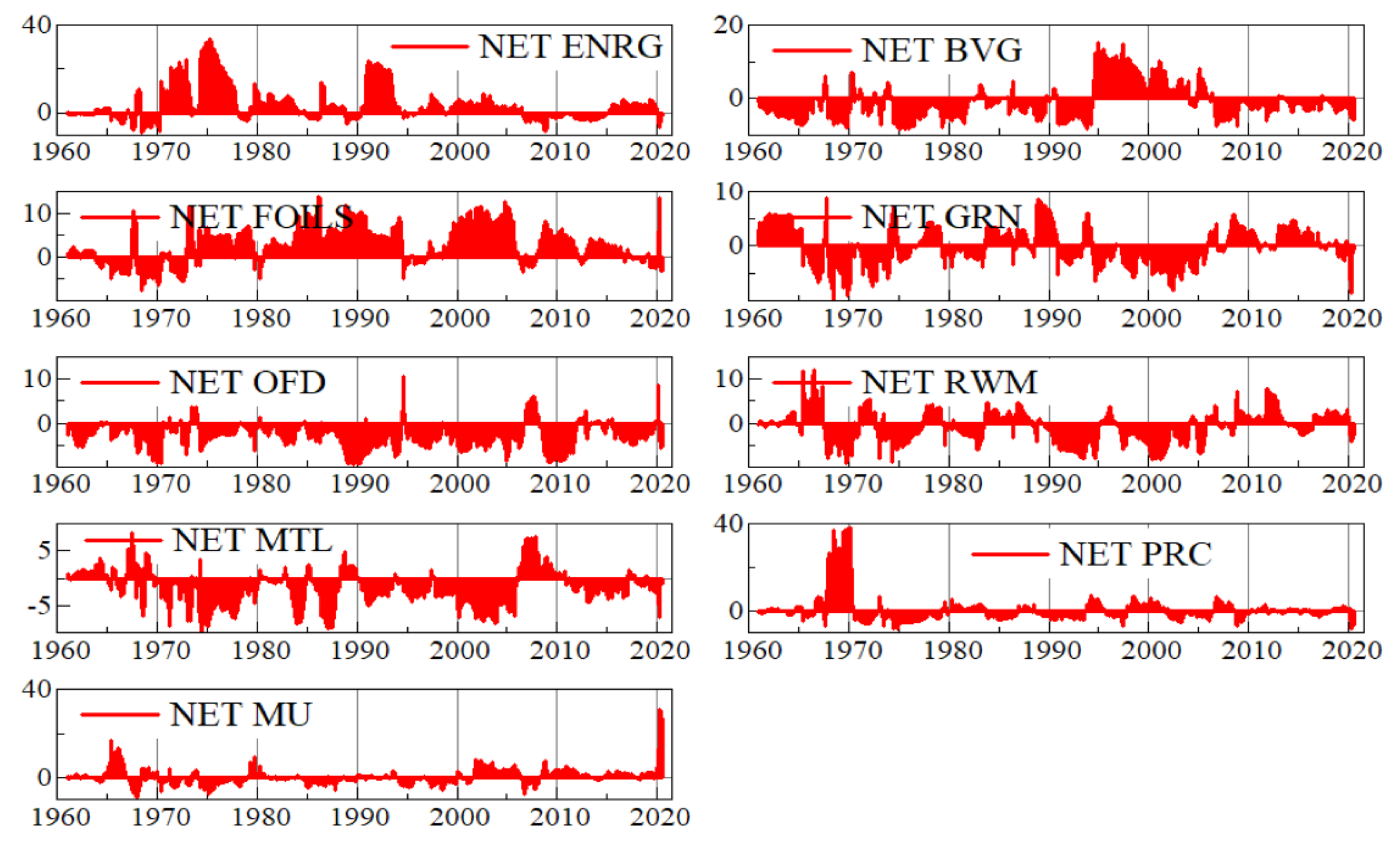
5.2.2. Net Pairwise Connectedness and Net Total Directional Connectedness Uncertainty
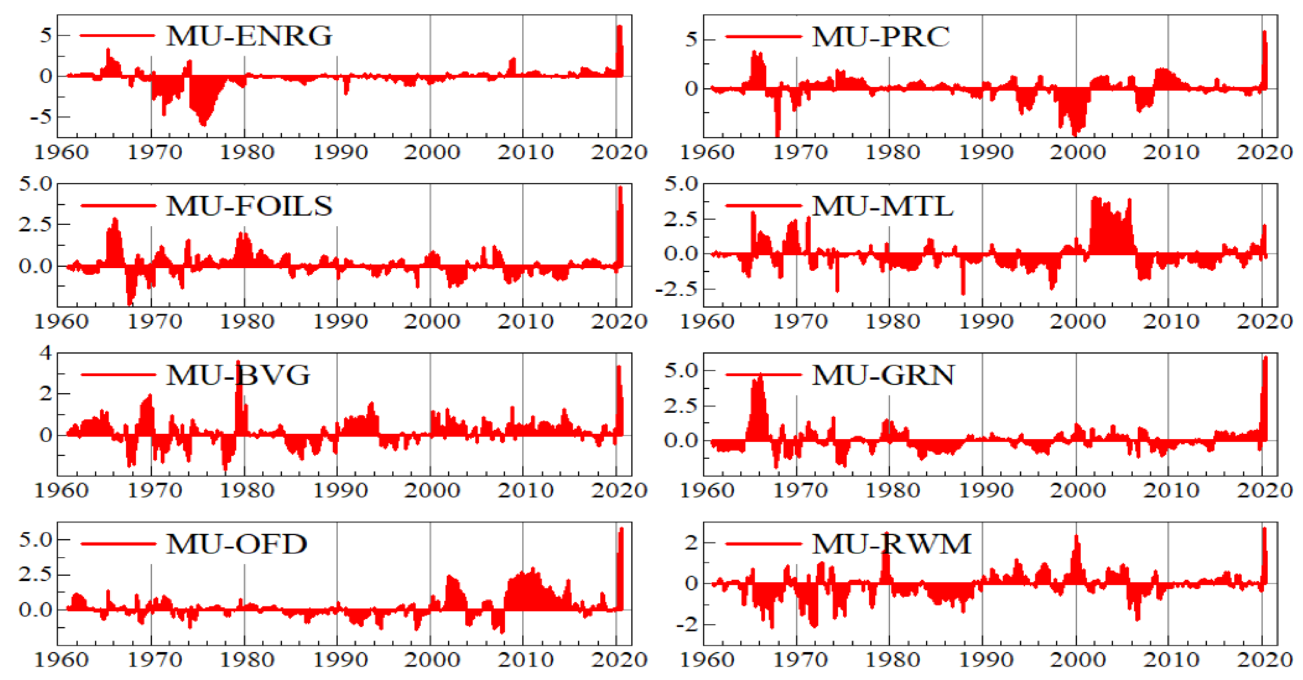
We calculate the net spillovers and the pairwise spillovers to obtain information about direction and intensity of uncertainty spillovers. The results are shown in Table 3 (total directional connectedness among commodity uncertainty markets and MU), Figure 7 (net total directional connectedness uncertainties), and Figure A1, Figure A2, Figure A3, Figure A4, Figure A5 and Figure A6 in Appendix B (net pairwise directional connectedness uncertainties). As our discussion of the dynamic connectedness in the previous section shows, the pairwise spillovers study corroborates the findings in Table 3 and confirms the supremacy of the energy uncertainty index over all commodity markets and the macroeconomic uncertainty index. Several interesting results are noted as follows. The pairwise spillovers results show that energy is a net transmitter of uncertainty to all commodities and to the macroeconomic uncertainty index, followed by Fats and Oils with a net spillover of 226.36% Other foods, Metals, Beverages, Raw materials, and Grains appear as net receivers of uncertainty from other markets. While macroeconomic uncertainty index and precious metal are considered as neutral during the overall sample period with a weak net spillover of 1.38% and 4.98%, respectively. Macroeconomic uncertainty is a net receiver from energy and Raw materials, and a net transmitter to the remaining commodities. This finding is in line with the results of Ji et al. (2018), Algieri and Leccadito (2017), who point out crude oil’s contagious effect on food price and explain that an upsurge in crude oil price may increase the price of corn and soybean that can be used to produce biodiesel and biofuel. Moreover, Barbaglia et al. (2020) reveal that higher volatility in natural gas and gasoline, or diesel prices used as input for fertilizers production and fuel, affect volatility in the agricultural market. Fats and Oils are a net transmitter of uncertainty to agricultural commodities but are considered a net receiver of uncertainty from Energy, Precious Metals, and the Macroeconomic uncertainty index.
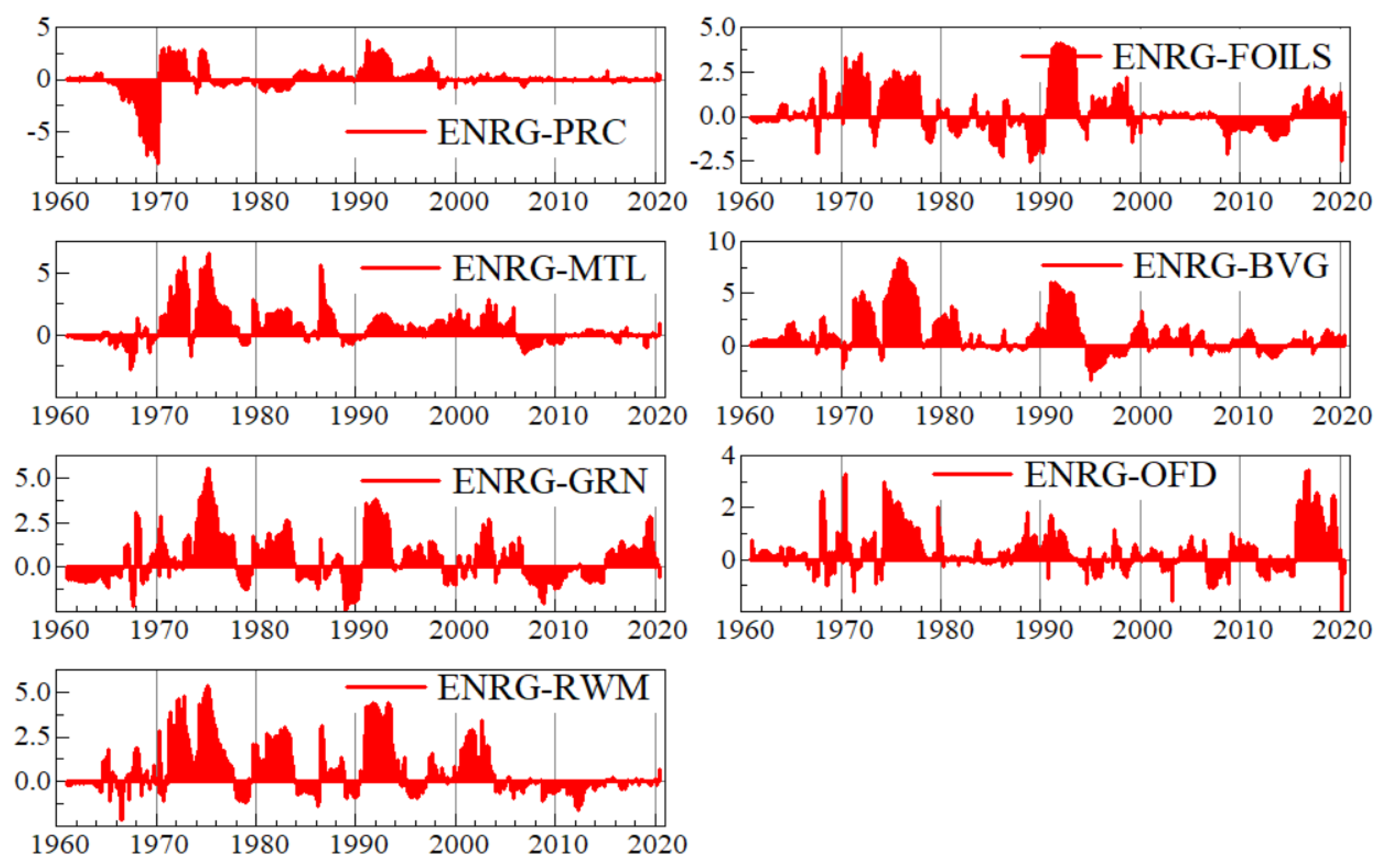
Next, we detect the net pairwise for three commodities and the macroeconomic uncertainty index transmitters of uncertainty shocks to other commodity markets. Figure A1 shows the macroeconomic uncertainty net pairwise with other commodity markets. The uncertainty effects of this index on other commodity markets are weak during the overall sample period but become the major transmitter of uncertainty from the end of the sample period with the advent of the COVID-19 pandemic that has caused an increase in risks and uncertainty and enormous economic damage. Figure A2 displays the dynamic net pairwise between Energy uncertainty and other commodity markets. The uncertainty shocks in Energy influence mostly the Fats and Oils, Metals, Beverages, Grains, Other foods, and Raw-Materials. We observe a bi-directional transmission of uncertainty between energy and Fats Oils, Metals, Beverages, Grains, Other Foods, and Raw-Materials, confirming the findings of Naeem et al. (2021). However, Energy is a slightly transmitter of uncertainty to the Precious Metal during overall our sample period and this confirms the safe-haven role assigned to the Precious Metals.
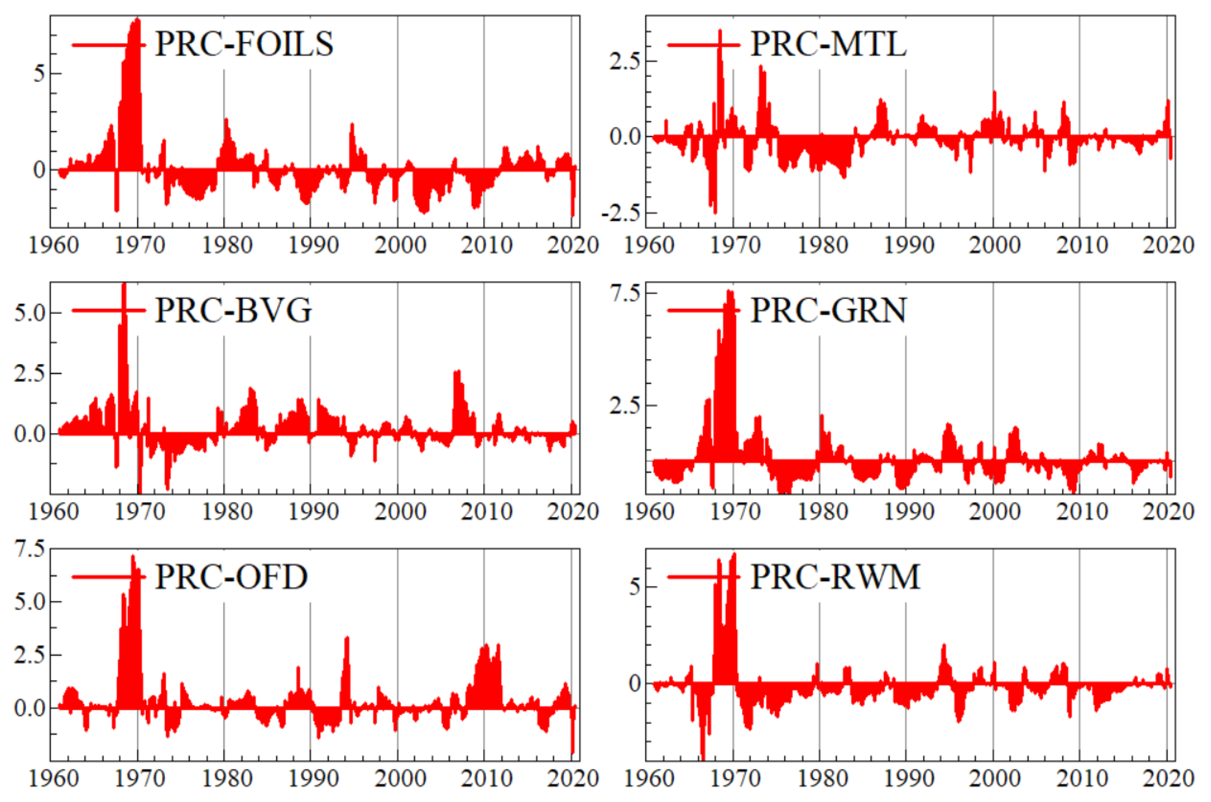
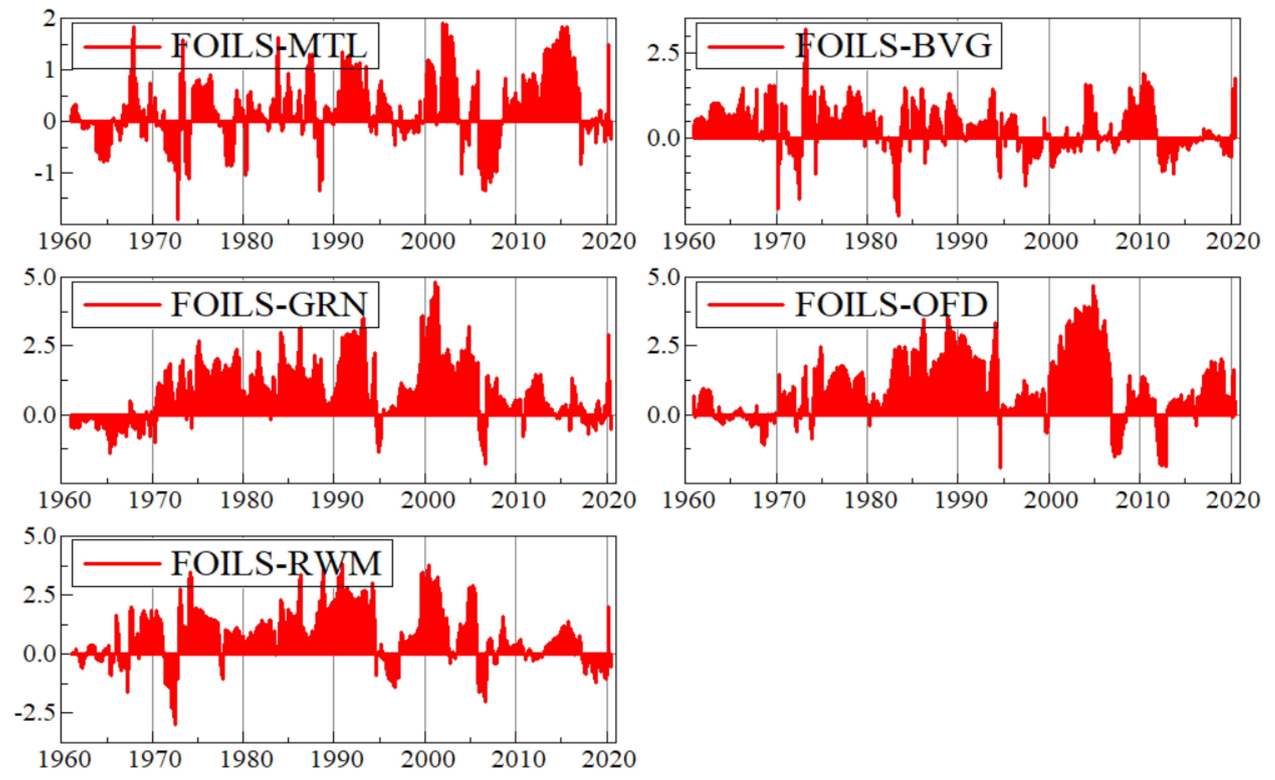
Figure A3 describes the precious metals uncertainty net pairwise spillover. We can see that the precious metals market is a transmitter of uncertainty to other commodity markets during the gold standard regime. Figure A4 shows the Fats and Oils uncertainty net pairwise with Metals, Beverages, Grains, Other Foods, and Raw Materials. Fats and Oils is a net transmitter of uncertainty to the agricultural commodities, and particularly for Grains, Other Foods, and Raw materials as presented in Table 3. This result is in line with the findings of Taghizadeh-Hesary et al. (2018), which reveals that the impact of biofuel prices on food prices is statistically significant but explains less than 2% of the food price variance.
5.2.3. Robustness Analysis
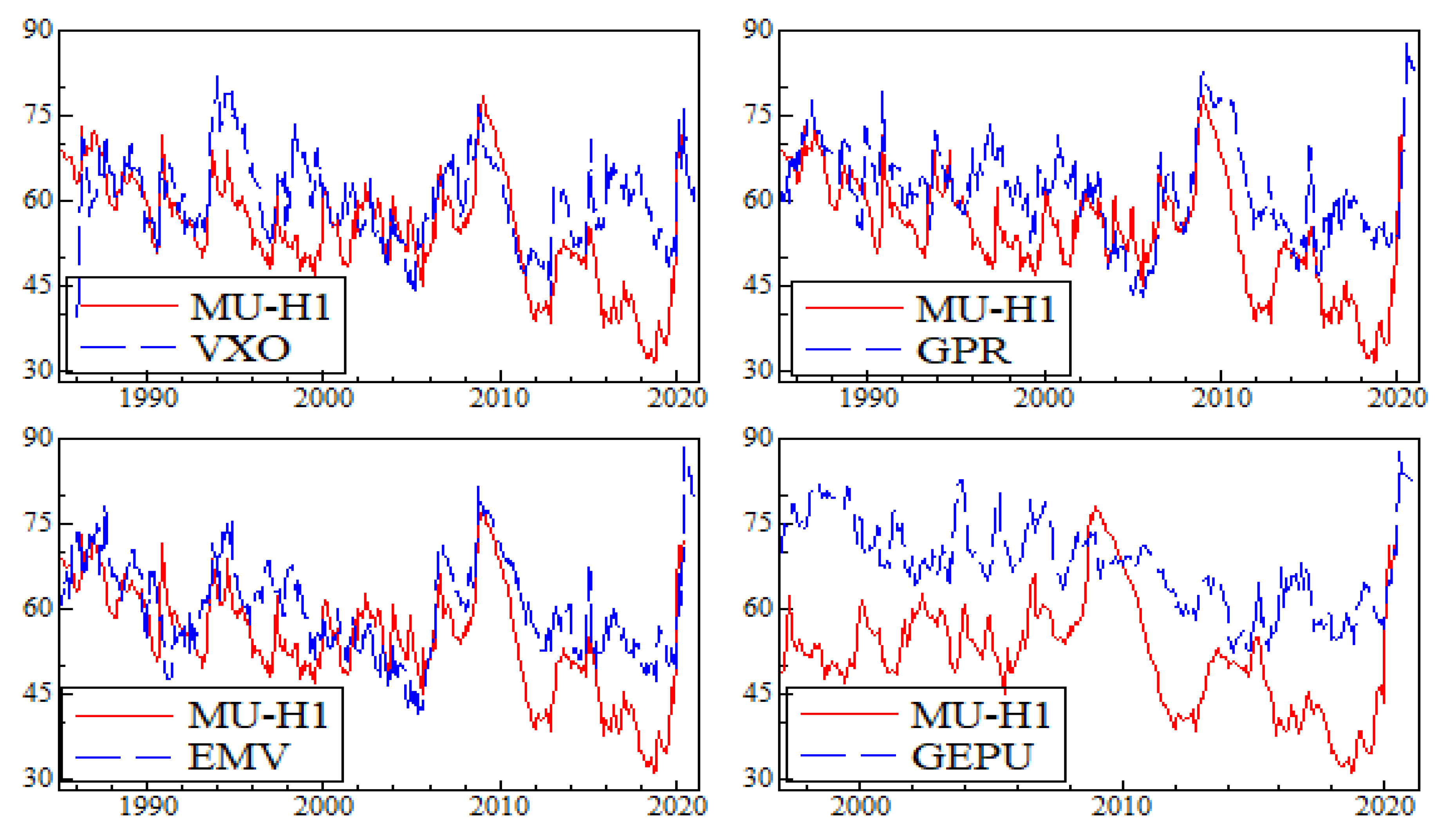
We undertake a robustness check by considering several alternative economic and financial uncertainty measures. First, we explore the robustness of our findings against several MU maturities, namely, 1, 3 and 12 months. Second, we examine the sensitivity of our findings to observable economic and financial uncertainty measures, namely the Global Economic Policy Uncertainty (GEPU, see Baker et al. 2016), the geopolitical risk index (GPR, see Caldara and Iacoviello 2018), the newspaper-based Equity Market Volatility (EMV, see Baker et al. 2016), and the CBOE S & P 100 Volatility Index (VXO).
Figure A7 in Appendix C reports the total directional connectedness across commodity uncertainties and different MU maturities (1, 3, and 12 months). The findings indicate that the total directional connectedness indices exhibit a similar pattern, whatever the maturity. Also, Figure A8 in Appendix C displays the estimated the total directional connectedness across commodity uncertainties and the observable economic and financial uncertainty measures. The findings suggest that extent of uncertainty connectedness is not sensitive to economic and financial uncertainty measures, except for the GPEU measure, where we observe that the latent MU proposed by Jurado et al. (2015) and the observable GPEU measure produce quite different total directional connectedness uncertainty indices. Thus, the alternative uncertainty measures do not seem to affect our main findings.
6. Conclusions
The recent strong volatility observed in the commodities markets raised the question about the efficient predictors of uncertainty in these markets. To address this question, this study sought to estimate, firstly, individual latent commodity price uncertainty for 8 main categories of commodity markets, namely energy, beverages, fats and oils, grains, other foods, raw materials, industrial metals, and precious metals. The period span is January 1960 to June 2020. The estimation of commodity price uncertainty is based on the approach of Jurado et al. (2015). Secondly, we examined the dynamic connectedness between commodity uncertainties and the Jurado et al.’s (2015) macroeconomic uncertainty index. To this end, we used the recent TVP-VAR-based dynamic connectedness approach proposed by Antonakakis et al. (2020).
Our findings show that the estimated commodity price uncertainties display few episodes of uncertainty, supporting the fact that uncertainty is related to predictability rather than volatility. Indeed, we have found that the 1970s, 1990s, 2007–2009, and the recent COVID-19 pandemic crises have caused the highest uncertainty episodes. Thus, the distinct commodity uncertainty estimates can detect the main episodes of heightened macroeconomic and financial uncertainty during the period 1960–2020. The findings are largely consistent with the results of Joëts et al. (2017) and Balli et al. (2019).
In addition, we have found that the time varying system price connectedness between the commodities markets increased during heightened economic and financial uncertainty periods. The energy uncertainty is the dominant shock that influences the other commodity markets and macroeconomic uncertainty. The latter does impact the commodity uncertainties only during the recent COVID-19 pandemic crisis. Moreover, the findings confirm the important role of precious metals as a safe-haven commodity during uncertainty periods. Finally, the fats and oils uncertainty is the main source of the various agriculture market uncertainties.
Hence, our estimated commodity price uncertainties are reliable tools to investors and policymakers to accurately predict uncertainty episodes. Besides, the connectedness analysis help investors to identify the disconnected commodity markets, and to manage portfolio diversification.
Despite the reliable economic implications of econometric results of the paper, some areas in the field need to be investigated. In this way, it would be suitable to extend this study by estimating commodity price uncertainty under short-and long-run co-movement restrictions. Indeed, extending the TVP-VAR model to account for both common cyclical and common trend features would help improve the techniques to forecast commodity price uncertainty.
Author Contributions
H.B.H.: Conceptualization, Methodology, Investigation, Software, Writing, Original Draft; I.M.: Methodology, Investigation, Formal analysis, Writing—Review & Editing; A.G.: Writing—Review & Editing, Investigation, Visualization, Validation. All authors have read and agreed to the published version of the manuscript.
Funding
This research was supported by the Deanship of Scientific Research, Imam Mohammad lbn Saud Islamic University, Saudi Arabia, Grant No. (20-13-11-012).
Institutional Review Board Statement
Not Applicable.
Informed Consent Statement
Not Applicable.
Data Availability Statement
Available upon request.
Acknowledgments
This research was supported by the Deanship of Scientific Research, Imam Mohammad lbn Saud Islamic University, Saudi Arabia, Grant No. (20-13-11-012).
Conflicts of Interest
The authors declare no conflict of interest.
Appendix A. Data Sources and Description

Table A1.
Commodity dataset. 1997M1–2019M6.
| Market | Description | Transformation | Source |
|---|---|---|---|
| Energy Market | Fuel (Energy) Index, 2010 = 100, includes Crude oil (petroleum), Natural Gas, Coal Price and Propane Indices. | ∆ln | WDI |
| Precious Metals Market | Precious Metals Price Index, 2010 = 100, includes Gold, Silver, Palladium and Platinum Price Indices | ∆ln | WDI |
| Beverage | Beverage Price Index, 2010 = 100, includes Coffee and Tea. | ∆ln | WDI |
| Fats Oils | Oils and Meals Price Index, 2010 = 100, includes Coconut oil, Copra, Fishmeal, Groundnuts, Groundnut oil, Palm oil, Palm kernel oil, Soybean meal, Soybean oil and Soybeans. | ∆ln | WDI |
| Grains | Grains Price Index, 2010 = 100, includes Barley, Maize, Rice, Sorghum and Wheat. | ∆ln | WDI |
| Other Food | Other Food Price index, 2010 = 100, includes Bananas, Meats (boeuf, chicken and sheep), Oranges, Shrimp and Sugars. | ∆ln | WDI |
| Raw Materials | Raw Materials Price index, 2010 = 100, includes Timber and other raw materials (Cotton, Rubber and Tobacco). | ∆ln | WDI |
| Metals and Minerals Market | Base Metals Price Index, 2010 = 100, includes Aluminium, Copper, Iron, Lead, Nickel, Steels, Tin and Zinc. | ∆ln | WDI |
| Macroeconomic Uncertainty (MU1) | The one-month macroeconomic uncertainty indicator proposed by Jurado et al. (2015) | https://www.sydneyludvigson.com/data-and-appendixes, (accessed on 20 December 2020) |
Note: ∆ln denotes the first-logarithmic difference transformation and WDI is the World Bank Commodity Price Data (The Pink Sheet).
Appendix B. Graphs of Net Pairwise Connectedness Uncertainties
Figure A1.
Macroeconomic Uncertainty Net Pairwise.

Figure A2.
Energy Uncertainty Net Pairwise.

Figure A3.
Precious Metals Uncertainty Net Pairwise.

Figure A4.
Fat Oils Uncertainty Net Pairwise.

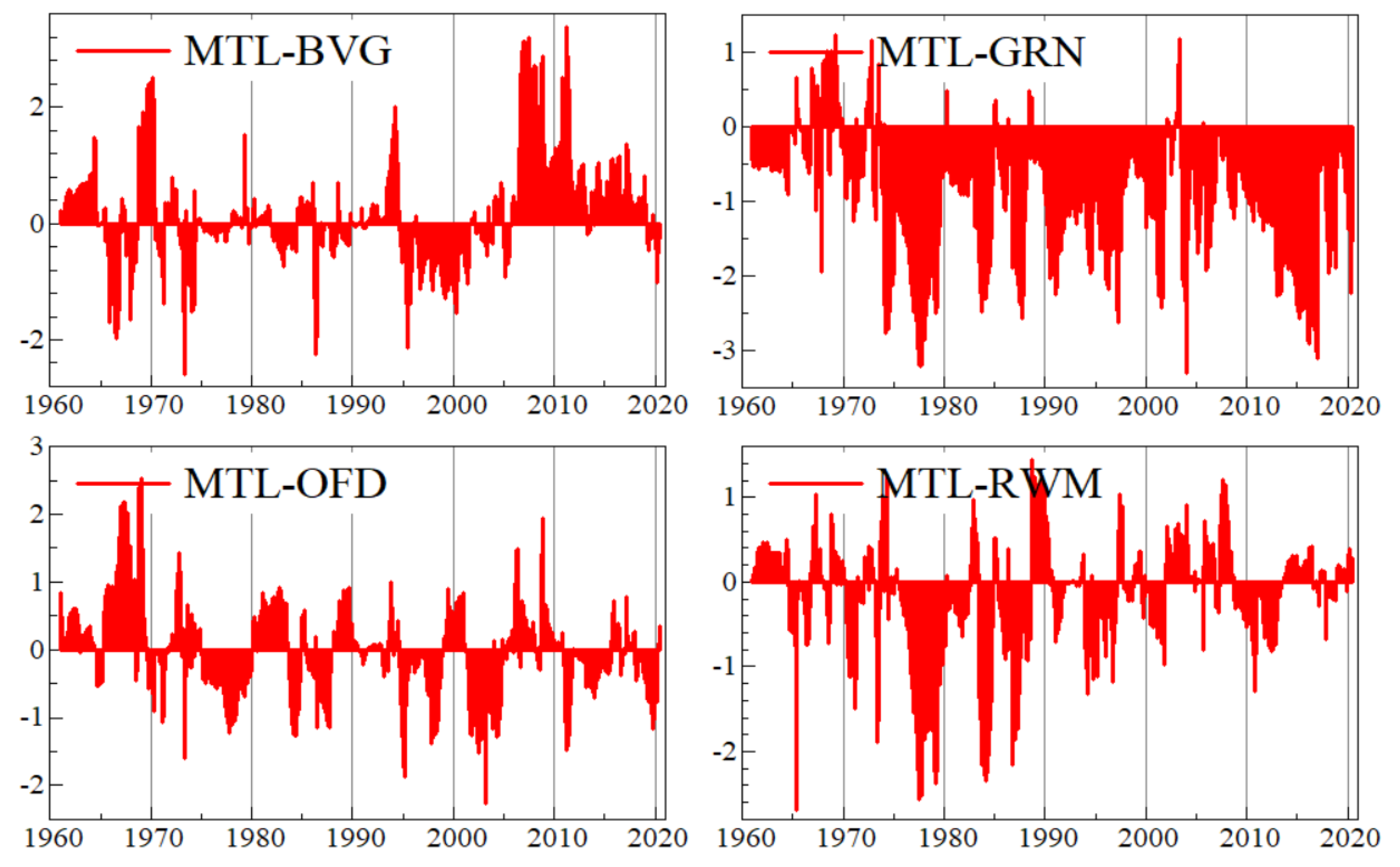
Figure A5.
Metals Uncertainty Net Pairwise.

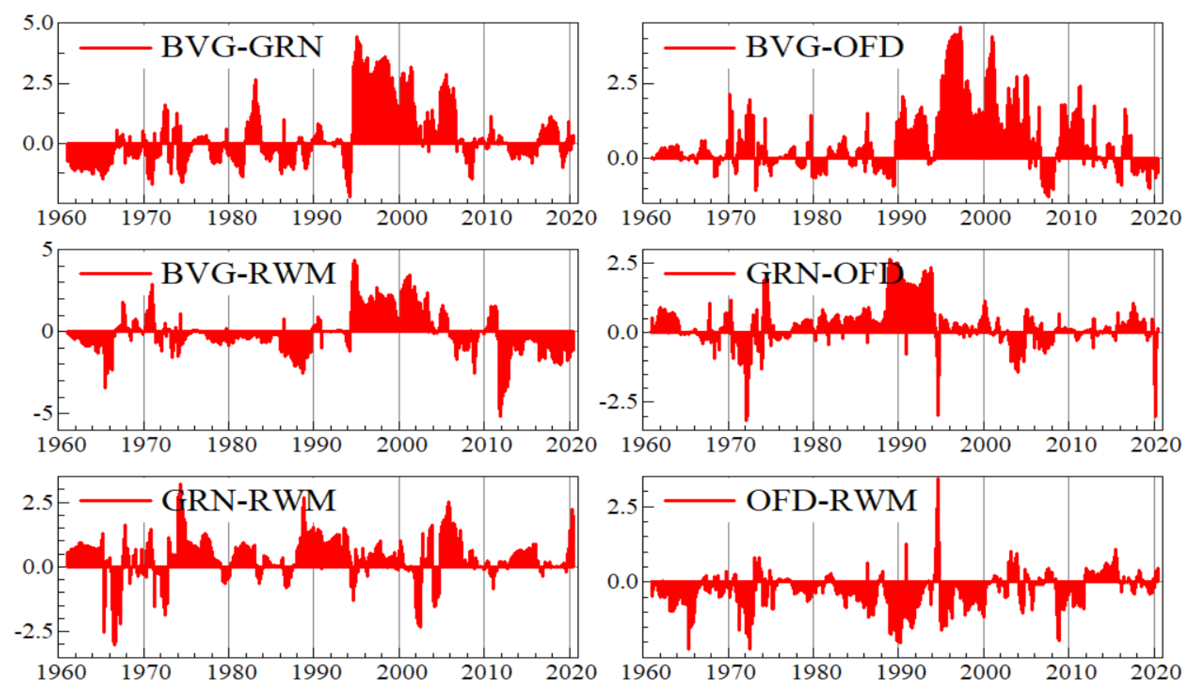
Figure A6.
Beverages, Grains, Other Food, and Raw Materials Uncertainty Net Pairwise.

Appendix C. Graphs of Robustness Analysis
Figure A7.
Total directional uncertainty connectedness index using different MU maturities.

Figure A8.
Total directional uncertainty connectedness index using various economic and financial uncertainty measures.
Figure A8.
Total directional uncertainty connectedness index using various economic and financial uncertainty measures.

References
- Ahumada, Hildegart, and Magdalena Cornejo. 2016. Forecasting food prices: The cases of corn, soybeans and wheat. International Journal of Forecasting 32: 838–48. [Google Scholar] [CrossRef]
- Algieri, Bernardina, and Arturo Leccadito. 2017. Assessing contagion risk from energy and non-energy commodity markets. Energy Economics 62: 312–22. [Google Scholar] [CrossRef]
- Alquist, Ron, and Lutz Kilian. 2010. What do we learn from the price of crude oil futures? Journal of Applied Econometrics 25: 539–73. [Google Scholar] [CrossRef] [Green Version]
- Antonakakis, Nikolaos, Ioannis Chatziantoniou, and David Gabauer. 2020. Refined measures of dynamic connectedness based on time-varying parameter vector autoregressions. Journal of Risk and Financial Management 13: 84. [Google Scholar] [CrossRef]
- Antonakakis, Nikolaos, Ioannis Chatziantoniou, and George Filis. 2014. Dynamic spillovers of oil price shocks and economic policy uncertainty. Energy Economics 44: 433–47. [Google Scholar] [CrossRef] [Green Version]
- Arouri, Mohamed El Hedi, Amine Lahiani, and Duc Khuong Nguyen. 2011a. Return and volatility transmission between world oil prices and stock markets of the GCC countries. Economic Modelling 28: 1815–25. [Google Scholar] [CrossRef] [Green Version]
- Arouri, Mohamed El Hedi, Jamel Jouini, and Duc Khuong Nguyen. 2011b. Volatility spillovers between oil prices and stock sector returns: Implications for portfolio management. Journal of International Money and Finance 30: 1387–405. [Google Scholar] [CrossRef]
- Badshah, Ihsan, Riza Demirer, and Muhammad Tahir Suleman. 2019. The effect of economic policy uncertainty on stock-commodity correlations and its implications on optimal hedging. Energy Economics 84: 104553. [Google Scholar] [CrossRef]
- Bahloul, Walid, Mehmet Balicilar, Juncal Cunado, and Gupta Rangan. 2018. The role of economic and financial uncertainties in predicting commodity futures returns and volatility: Evidence from a nonparametric causality-in-quantiles test. Journal of Multinational Financial Management 45: 52–71. [Google Scholar] [CrossRef]
- Bai, Jushan, and Serena Ng. 2002. Determining the number of factors in approximate factor models. Econometrica 70: 191–221. [Google Scholar] [CrossRef] [Green Version]
- Bakas, Dimitrios, and Athanasios Triantafyllou. 2018. The impact of uncertainty shocks on the volatility of commodity prices. Journal of International Money and Finance 87: 96–111. [Google Scholar] [CrossRef] [Green Version]
- Bakas, Dimitrios, and Athanasios Triantafyllou. 2019. Volatility forecasting in commodity markets using macro uncertainty. Energy Economics 81: 79–94. [Google Scholar] [CrossRef]
- Bakas, Dimitrios, and Athanasios Triantafyllou. 2020. Commodity price volatility and the economic uncertainty of pandemics. Economics Letters 193: 109283. [Google Scholar] [CrossRef]
- Baker, Scott R., Nicholas Bloom, and Steven J. Davis. 2016. Measuring economic policy uncertainty. The Quarterly Journal of Economics 131: 1593–636. [Google Scholar] [CrossRef]
- Balli, Faruk, Muhammad Abubakr Naeem, and Syed Jawad Hussain Shahzad. 2019. Spillover network of commodity uncertainties. Energy Economics 81: 914–27. [Google Scholar] [CrossRef]
- Barbaglia, Luca, Christophe Croux, and Ines Wilms. 2020. Volatility spillovers in commodity markets: A large t-vector autoregressive approach. Energy Economics 85: 104555. [Google Scholar] [CrossRef]
- Baumeister, Christiane, and Lutz Kilian. 2012. Real-time forecasts of the real price of oil. Journal of Business and Economic Statistics 30: 326–36. [Google Scholar] [CrossRef] [Green Version]
- Baumeister, Christiane, and Lutz Kilian. 2015. Forecasting the real price of oil in a changing world: A forecast combination approach. Journal of Business and Economic Statistics 33: 338–51. [Google Scholar] [CrossRef] [Green Version]
- Baumeister, Christine, Lutz Kilian, and Xiaoqing Zhou. 2018. Are product spreads useful for forecasting oil prices? an empirical evaluation of the Verleger hypothesis. Macroeconomic Dynamics 22: 562–80. [Google Scholar] [CrossRef]
- Bekiros, Stelios, Rangan Gupta, and Alessia Paccagnini. 2015. Oil price forecast ability and economic uncertainty. Economic Letters 132: 125–28. [Google Scholar] [CrossRef] [Green Version]
- Bessembinder, Hendrik, and Kalok Chan. 2016. Time-varying risk premia and forecastable returns in futures markets. Journal of Financial Economic 32: 169–93. [Google Scholar] [CrossRef]
- Caldara, Dario, and Matteo Iacoviello. 2018. Measuring Geopolitical Risk. FRB International Finance Discussion Paper 1222. Available online: https://ssrn.com/abstract=3117773 (accessed on 20 December 2020).
- Chen, Yu-Chin, Kenneth S. Rogoff, and Barbara Rossi. 2010. Can Exchange Rates Forecast Commodity Prices? The Quarterly Journal of Economics 125: 1145–94. [Google Scholar] [CrossRef] [Green Version]
- Coppola, Andrea. 2008. Forecasting oil price movements: Exploiting the information in the futures market. Journal of Futures Markets 28: 34–56. [Google Scholar] [CrossRef]
- Diebold, Francis X., and Kamil Yilmaz. 2014. On the network topology of variance decompositions: Measuring the connectedness of financial firms. Journal of Econometrics 182: 119–34. [Google Scholar] [CrossRef] [Green Version]
- Diebold, Francis X., Laura Liu, and Kamil Yilmaz. 2017. Commodity Connectedness. No. w23685. National Bureau of Economic Research. Available online: https://www.nber.org/papers/w23685 (accessed on 20 December 2020).
- Du, Xiaodong, L. Yu Cindy, and Dermot J. Hayes. 2011. Speculation and volatility spillover in the crude oil and agricultural commodity markets: A Bayesian analysis. Energy Economics 33: 497–503. [Google Scholar] [CrossRef]
- Elliott, Graham, Thomas J. Rothenberg, and James H. Stock. 1996. Efficient Tests for an Autoregressive Unit Root. Econometrica 64: 813–36. [Google Scholar] [CrossRef] [Green Version]
- Gankhuyag, Uyanga, and Fabrice Gregoire. 2018. Managing Mining for Sustainable Development: A Sourcebook. New York: United Nations Development Programme. [Google Scholar]
- Groen, Jan J. J., and Paolo A. Pesenti. 2011. Commodity prices, commodity currencies, and global economic developments. In Commodity Prices and Markets, East Asia Seminar on Economics. Edited by Takatoshi Ito and Andrew K. Rose. Chicago: University of Chicago Press, vol. 20, pp. 15–42. [Google Scholar]
- Hergt, Brian. 2013. Gold Prices during and after the Great Recession; Washington, DC: Bureau of Labor Statistics.
- Hong, Harrison, and Motohiro Yogo. 2012. What does futures market interest tell us about the macroeconomy and asset prices? Journal of Financial Economic 105: 473–90. [Google Scholar] [CrossRef] [Green Version]
- Jarque, Carlos M., and Anil K. Bera. 1980. Efficient tests for normality, homoscedasticity and serial independence of regression residuals. Economics letters 6: 255–59. [Google Scholar] [CrossRef]
- Ji, Qiang, Elie Bouri, David Roubaud, and Syed J. H. Shahzad. 2018. Risk spillover between energy and agricultural commodity markets: A dependence-switching CoVaR-copula model. Energy Economics 75: 14–27. [Google Scholar] [CrossRef]
- Joëts, Marc, Valérie Mignon, and Tovonony Razafindrabe. 2017. Does the volatility of commodity prices reflect macroeconomic uncertainty? Energy Economics 68: 313–26. [Google Scholar] [CrossRef]
- Jurado, Kyle, Sydney C. Ludvigson, and Serena Ng. 2015. Measuring uncertainty. American Economic Review 105: 1177–216. [Google Scholar] [CrossRef]
- Kang, Sang Hoon, Ron McIver, and Seong-Min Yoon. 2017. Dynamic spillover effects among crude oil, precious metal, and agricultural commodity futures markets. Energy Economics 62: 19–32. [Google Scholar] [CrossRef]
- Kang, Wensheng, and Ronald A. Ratti. 2013. Oil shocks, policy uncertainty and stock market return. Journal of International Financial Markets, Institutions and Money 26: 305–18. [Google Scholar] [CrossRef]
- Koop, Gary, M. Hashem Pesaran, and Simon M. Potter. 1996. Impulse response analysis in nonlinear multivariate models. Journal of econometrics 74: 119–47. [Google Scholar] [CrossRef]
- Korobilis, Dimitris, and Kamil Yilmaz. 2018. Measuring Dynamic Connectedness with Large Bayesian VAR Models. Available online: https://ssrn.com/abstract=3099725 (accessed on 12 December 2020).
- Krugman, Paul. 2008. The oil nonbubble. New York Times, May 12. [Google Scholar]
- Kuhns, Annemarie, and Abigail Okrent. 2019. Factors Impacting Grocery Store Deflation: A Closer Look at Prices in 2016 and 2017; EB-28. Washington, DC: U.S. Department of Agriculture, Economic Research Service.
- Ljung, Greta M., and George E. P. Box. 1978. On a measure of lack of fit in time series models. Biometrika 65: 297–303. [Google Scholar] [CrossRef]
- Mensi, Walid, Makram Beljid, Adel Boubaker, and Managi Shunsuke. 2013. Correlations and volatility spillovers across commodity and stock markets: Linking energies, food, and gold. Economic Modelling 32: 15–22. [Google Scholar] [CrossRef] [Green Version]
- Naeem, Muhammad Abubakr, Saqib Farid, Safwan Mohd Nor, and Syed Jawad Hussain Shahzad. 2021. Spillover and Drivers of Uncertainty among Oil and Commodity Markets. Mathematics 9: 441. [Google Scholar] [CrossRef]
- Pesaran, H. Hashem, and Yongcheol Shin. 1998. Generalized impulse response analysis in linear multivariate models. Economics Letters 58: 17–29. [Google Scholar] [CrossRef]
- Poncela, Pilar, Eva Senra, and Lya Paola Sierra. 2014. Common dynamics of nonenergy commodity prices and their relation to uncertainty. Applied Economics 46: 3724–35. [Google Scholar] [CrossRef]
- Shiferaw, Yegnanew A. 2019. Time-varying correlation between agricultural commodity and energy price dynamics with Bayesian multivariate DCC-GARCH models. Physica A: Statistical Mechanics and Its Applications 526: 120807. [Google Scholar] [CrossRef]
- Silvennoinen, Annastiina, and Susan Thorp. 2013. Financialization, crisis and commodity correlation dynamics. Journal of International Financial Markets, Institutions and Money 24: 42–65. [Google Scholar] [CrossRef] [Green Version]
- Stuermer, Martin. 2018. 150 years of boom and bust: What drives mineral commodity prices? Macroeconomic Dynamics 22: 702–17. [Google Scholar] [CrossRef] [Green Version]
- Taghizadeh-Hesary, Farhad, Ehsan Rasoulinezhad, and Naoyuki Yoshino. 2018. Volatility Linkages between Energy and Food Prices: Case of Selected Asian Countries. Asian Development Bank Institute. Available online: http://hdl.handle.net/11540/8113 (accessed on 20 December 2020).
- Van Robays, Ine. 2016. Macroeconomic uncertainty and oil price volatility. Oxford Bulletin of Economics and Statistics 78: 671–93. [Google Scholar] [CrossRef]
- Wang, Yudong, Bing Zhang, Xundi Diao, and Chongfeng Wu. 2015. Commodity price changes and the predictability of economic policy uncertainty. Economic Letters 27: 39–42. [Google Scholar] [CrossRef]
- Wang, Yudong, Li Liu, and Chongfeng Wu. 2017. Forecasting the real prices of crude oil using forecast combinations over time-varying parameter models. Energy Economics 66: 337–48. [Google Scholar] [CrossRef]
- Watugala, Sumudu W. 2019. Economic uncertainty, trading activity, and commodity futures volatility. Journal of Futures Markets 39: 921–45. [Google Scholar] [CrossRef]
- Wiggins, Steve, Sharada Keats, and Julia Compton. 2010. What Caused the Food Price Spike of 2007/08? Lessons for World Cereals Markets. Food Prices Project Report. London: Overseas Development Institute, Available online: www.odi.org.uk (accessed on 20 December 2020).
- Yang, Lu. 2019. Connectedness of economic policy uncertainty and oil price shocks in a time domain perspective. Energy Economics 80: 219–33. [Google Scholar] [CrossRef]
- Ye, Michael, John Zyren, and Joanne Shore. 2006. Forecasting short-run crude oil price using high- and low inventory variables. Energy Policy 34: 2736–43. [Google Scholar] [CrossRef]
- Yin, Libo, and Liyan Han. 2014. Macroeconomic uncertainty: Does it matter for commodity prices? Applied Economics Letters 21: 711–16. [Google Scholar] [CrossRef]
- Zhu, Huiming, Huang Rui, Wang Ningli, and Liya Hau. 2020. Does economic policy uncertainty matter for commodity market in China? Evidence from quantile regression. Applied Economics 52: 2292–308. [Google Scholar] [CrossRef]
- Zivot, Eric, and Donald W. K. Andrews. 1992. Further evidence on the great crash, the oil-price shock, and the unit-root hypothesis. Journal of Business & Economic Statistics 10: 251–70. [Google Scholar]
Figure 1.
The Jurado et al. (2015) macroeconomic uncertainty measure. The dashed area represents the NBER recession dates.
Figure 1.
The Jurado et al. (2015) macroeconomic uncertainty measure. The dashed area represents the NBER recession dates.

Figure 2.
Energy uncertainty index. The dashed horizontal bars correspond to 1.65 standard deviations above the mean, and the dashed area represents the NBER recession dates.
Figure 2.
Energy uncertainty index. The dashed horizontal bars correspond to 1.65 standard deviations above the mean, and the dashed area represents the NBER recession dates.

Figure 3.
Precious metals uncertainty index. The dashed horizontal bars correspond to 1.65 standard deviations above the mean, and the dashed area represents the NBER recession dates.
Figure 3.
Precious metals uncertainty index. The dashed horizontal bars correspond to 1.65 standard deviations above the mean, and the dashed area represents the NBER recession dates.

Figure 4.
Industrial metals uncertainty index. The dashed horizontal bars correspond to 1.65 standard deviations above the mean, and the dashed area represents the NBER recession dates.
Figure 4.
Industrial metals uncertainty index. The dashed horizontal bars correspond to 1.65 standard deviations above the mean, and the dashed area represents the NBER recession dates.

Figure 5.
Agriculture uncertainty indices. The dashed horizontal bars correspond to 1.65 standard deviations above the mean, and the dashed area represents the NBER recession dates.
Figure 5.
Agriculture uncertainty indices. The dashed horizontal bars correspond to 1.65 standard deviations above the mean, and the dashed area represents the NBER recession dates.


Figure 6.
Total directional uncertainty connectedness index.

Figure 7.
Net total directional connectedness uncertainty.

Table 1.
Descriptive Statistics of Commodity Price Returns.
| ENRG | BVG | FOILS | GRN | OFD | RWM | MTL | PRC | ||
| Mean | 0.005 | 0.002 | 0.002 | 0.002 | 0.002 | 0.002 | 0.003 | 0.005 | |
| Variance | 0.006 | 0.002 | 0.002 | 0.002 | 0.002 | 0.001 | 0.002 | 0.002 | |
| Skewness | 3.177 *** | 0.920 *** | 0.236 *** | 0.610 *** | 0.384 *** | 0.464 *** | −0.669 *** | 1.283 *** | |
| Kurtosis | 50.725 *** | 4.839 *** | 5.701 *** | 4.228 *** | 3.481 *** | 3.604 *** | 4.998 *** | 14.115 *** | |
| JB | 79,925.904 *** | 819.528 *** | 1000.643 *** | 592.273 *** | 388.639 *** | 423.559 *** | 818.878 *** | 6294.725 *** | |
| ERS | −7.629 *** | −5.793 *** | −4.038 *** | −5.733 *** | −7.755 *** | −7.175 *** | −7.379 *** | −5.711 *** | |
| Q(20) | 44.339 *** | 87.345 *** | 121.306 *** | 131.686 *** | 40.137 *** | 162.328 *** | 96.979 *** | 85.884 *** | |
| Q2(20) | 0.051 | 36.616 *** | 166.420 *** | 109.891 *** | 60.371 *** | 47.470 *** | 37.348 *** | 13.221 | |
| LM(20) | 8.258 | 44.900 *** | 90.204 *** | 24.629 *** | 64.579 *** | 38.758 *** | 23.000 *** | 89.312 *** | |
| Z-A Unit Root Test | |||||||||
| ENRG | BVG | FOILS | GRN | OFD | RWM | MTL | PRC | MU | |
| T-Statistics | −21.339 *** | −15.158 *** | −17.242 *** | −18.469 *** | −22.402 *** | −18.132 *** | −19.547 *** | −19.574 *** | −5.8119 *** |
| Break date | 11/1979 | 3/1977 | 10/1974 | 2/1974 | 11/1974 | 2/2011 | 6/1988 | 1/1980 | 1/1983 |
| Unconditional Correlations | |||||||||
| ENRG | BVG | FOILS | GRN | OFD | RWM | MTL | PRC | ||
| ENRG | 1 | 0.168 | 0.155 | 0.069 | 0.144 | 0.226 | 0.255 | 0.192 | |
| BVG | 0.168 | 1 | 0.217 | 0.111 | 0.129 | 0.158 | 0.201 | 0.158 | |
| FOILS | 0.155 | 0.217 | 1 | 0.459 | 0.192 | 0.218 | 0.239 | 0.228 | |
| GRN | 0.069 | 0.111 | 0.459 | 1 | 0.194 | 0.192 | 0.171 | 0.109 | |
| OOFD | 0.144 | 0.129 | 0.192 | 0.194 | 1 | 0.085 | 0.188 | 0.207 | |
| RWM | 0.226 | 0.158 | 0.218 | 0.192 | 0.085 | 1 | 0.253 | 0.223 | |
| MTL | 0.255 | 0.201 | 0.239 | 0.171 | 0.188 | 0.253 | 1 | 0.294 | |
| PRC | 0.192 | 0.158 | 0.228 | 0.109 | 0.207 | 0.223 | 0.294 | 1 | |
Notes: *** denotes significance at 1% significance level; JB: Jarque and Bera (1980) normality test; ERS: Elliott et al. (1996) unit-root test; Q(20) and Q2(20): Ljung and Box (1978) portmanteau test. Z-A: Zivot and Andrews (1992).
Table 2.
Descriptive Statistics of Uncertainty Indices.
| MU | ENRG | PRC | FOILS | MTL | BVG | GRN | OFD | RWM | |
| Mean | 0.646 | 1.049 | 1.201 | 1.529 | 1.267 | 1.388 | 1.298 | 1.420 | 1.802 |
| Variance | 0.009 | 0.014 | 0.125 | 0.143 | 0.065 | 0.083 | 0.065 | 0.114 | 0.254 |
| Skewness | 1.82 *** | 3.13 *** | 1.81 *** | 2.19 *** | 1.47 *** | 1.41 *** | 1.51 *** | 4.25 *** | 2.59 *** |
| Kurtosis | 3.87 *** | 25.07 *** | 6.97 *** | 5.54 *** | 3.73 *** | 3.51 *** | 3.63 *** | 24.36 *** | 7.95 *** |
| JB | 839.52 *** | 19,898.55 *** | 1838.95 *** | 1487.25 *** | 671.11 *** | 600.06 *** | 666.28 *** | 19,763.66 *** | 2682.87 *** |
| ERS | −3.64 *** | −2.22 ** | −1.83 * | −2.99 *** | −2.00 *** | −2.00 *** | −2.81 *** | −4.66 *** | −3.68 *** |
| Q(20) | 4353.09 *** | 2593.04 *** | 4196.53 *** | 4986.86 *** | 4646.22 *** | 4083.47 ** | 5412.72 *** | 3732.51 *** | 4644.32 *** |
| Q2(20) | 3344.93 *** | 1867.25 *** | 4192.82 *** | 3678.16 *** | 3882.19 *** | 2787.20 *** | 3458.23 *** | 1322.36 *** | 2474.62 *** |
| Unconditional Correlations | |||||||||
| MU | ENRG | PRC | FOILS | MTL | BVG | GRN | OFD | RWM | |
| MU | 1 | 0.337 | 0.681 | 0.404 | 0.381 | 0.15 | 0.399 | 0.289 | 0.318 |
| ENRG | 0.337 | 1 | 0.293 | 0.25 | 0.401 | 0.236 | 0.51 | −0.053 | 0.377 |
| PRC | 0.681 | 0.293 | 1 | 0.352 | 0.327 | 0.178 | 0.392 | 0.198 | 0.28 |
| FOILS | 0.404 | 0.25 | 0.352 | 1 | 0.363 | 0.34 | 0.677 | 0.443 | 0.36 |
| MTL | 0.381 | 0.401 | 0.327 | 0.363 | 1 | 0.129 | 0.633 | −0.039 | 0.583 |
| BVG | 0.15 | 0.236 | 0.178 | 0.34 | 0.129 | 1 | 0.312 | 0.187 | 0.064 |
| GRN | 0.399 | 0.51 | 0.392 | 0.677 | 0.633 | 0.312 | 1 | 0.104 | 0.682 |
| OFD | 0.289 | −0.053 | 0.198 | 0.443 | −0.039 | 0.187 | 0.104 | 1 | −0.029 |
| RWM | 0.318 | 0.377 | 0.28 | 0.36 | 0.583 | 0.064 | 0.682 | −0.029 | 1 |
Notes: ***, **, and * denote significance at 1%, 5%, and 10% significance levels, respectively; JB: Jarque and Bera (1980) normality test; ERS: Elliott et al. (1996) unit-root test; Q(20) and Q2(20): Ljung and Box (1978) portmanteau test.
Table 3.
Dynamic connectedness.
| MU | ENRG | PRC | FOILS | MTL | BVG | GRN | OFD | RWM | FROM | |
| MU | 48.068 | 7.706 | 9.549 | 6.088 | 7.329 | 4.884 | 5.933 | 4.369 | 6.073 | 51.932 |
| ENRG | 5.26 | 51.614 | 7.215 | 6.279 | 4.901 | 6.011 | 7.235 | 4.284 | 7.2 | 48.386 |
| PRC | 9.564 | 7.335 | 45.71 | 7.963 | 6.136 | 4.478 | 6.45 | 4.606 | 7.757 | 54.29 |
| FOILS | 6.565 | 8.942 | 8.721 | 42.518 | 5.117 | 5.211 | 10.988 | 5.451 | 6.487 | 57.482 |
| MTL | 7.34 | 10.752 | 5.451 | 7.334 | 34.613 | 5.318 | 14.834 | 6.208 | 8.15 | 65.387 |
| BVG | 6.304 | 15.614 | 6.569 | 8.349 | 6.928 | 35.223 | 7.275 | 5.13 | 8.608 | 64.777 |
| GRN | 6.549 | 11.395 | 7.57 | 19.183 | 5.701 | 9.318 | 26.496 | 5.458 | 8.331 | 73.504 |
| OFD | 6.579 | 7.492 | 7.812 | 14.924 | 5.87 | 10.172 | 7.723 | 31.571 | 7.856 | 68.429 |
| RWM | 5.156 | 13.317 | 6.385 | 13.721 | 6.261 | 7.445 | 11.656 | 4.999 | 31.06 | 68.94 |
| Contribution TO others | 53.318 | 82.553 | 59.271 | 83.841 | 48.244 | 52.839 | 72.095 | 40.504 | 60.462 | 553.127 |
| Contribution including own | 101.387 | 134.167 | 104.982 | 126.359 | 82.857 | 88.062 | 98.59 | 72.075 | 91.521 | |
| Net spillovers | 1.387 | 34.167 | 4.982 | 26.359 | −17.143 | −11.938 | −1.41 | −27.925 | −8.479 | TCI = 61.46% |
| Net Pairwises | ||||||||||
| MU | 0 | −2.446 | 0.015 | 0.477 | 0.011 | 1.42 | 0.616 | 2.21 | −0.917 | 1.386 |
| ENRG | 2.446 | 0 | 0.12 | 2.663 | 5.851 | 9.603 | 4.16 | 3.208 | 6.117 | 34.168 |
| PRC | −0.015 | −0.12 | 0 | 0.758 | −0.685 | 2.091 | 1.12 | 3.206 | −1.372 | 4.983 |
| FOILS | −0.477 | −2.663 | −0.758 | 0 | 2.217 | 3.138 | 8.195 | 9.473 | 7.234 | 26.359 |
| MTL | −0.011 | −5.851 | 0.685 | −2.217 | 0 | 1.61 | −9.133 | −0.338 | −1.889 | −17.144 |
| BVG | −1.42 | −9.603 | −2.091 | −3.138 | −1.61 | 0 | 2.043 | 5.042 | −1.163 | −11.940 |
| GRN | −0.616 | −4.16 | −1.12 | −8.195 | 9.133 | −2.043 | 0 | 2.265 | 3.325 | −1.411 |
| OFD | −2.21 | −3.208 | −3.206 | −9.473 | 0.338 | −5.042 | −2.265 | 0 | −2.857 | −27.923 |
| RWM | 0.917 | −6.117 | 1.372 | −7.234 | 1.889 | 1.163 | −3.325 | 2.857 | 0 | −8.478 |
Notes: Variance decomposition shares for estimated TVP-VAR (1), and the variance decompositions are based on 20-month-ahead forecasts.
Publisher’s Note: MDPI stays neutral with regard to jurisdictional claims in published maps and institutional affiliations. |
© 2021 by the authors. Licensee MDPI, Basel, Switzerland. This article is an open access article distributed under the terms and conditions of the Creative Commons Attribution (CC BY) license (https://creativecommons.org/licenses/by/4.0/).
Share and Cite
MDPI and ACS Style
Ben Haddad, H.; Mezghani, I.; Gouider, A. The Dynamic Spillover Effects of Macroeconomic and Financial Uncertainty on Commodity Markets Uncertainties. Economies 2021, 9, 91. https://0-doi-org.brum.beds.ac.uk/10.3390/economies9020091
AMA Style
Ben Haddad H, Mezghani I, Gouider A. The Dynamic Spillover Effects of Macroeconomic and Financial Uncertainty on Commodity Markets Uncertainties. Economies. 2021; 9(2):91. https://0-doi-org.brum.beds.ac.uk/10.3390/economies9020091
Chicago/Turabian StyleBen Haddad, Hedi, Imed Mezghani, and Abdessalem Gouider. 2021. "The Dynamic Spillover Effects of Macroeconomic and Financial Uncertainty on Commodity Markets Uncertainties" Economies 9, no. 2: 91. https://0-doi-org.brum.beds.ac.uk/10.3390/economies9020091
Note that from the first issue of 2016, this journal uses article numbers instead of page numbers. See further details here.