
E-Learning at-Risk Group Prediction Considering the Semester and Realistic Factors


1
College of Business Administration, Kookmin University, Seoul 02707, Republic of Korea
2
Graduate School of Business IT, Kookmin University, Seoul 02707, Republic of Korea
*
Author to whom correspondence should be addressed.
Educ. Sci. 2023, 13(11), 1130; https://0-doi-org.brum.beds.ac.uk/10.3390/educsci13111130
Submission received: 31 August 2023
/
Revised: 8 November 2023
/
Accepted: 11 November 2023
/
Published: 13 November 2023
(This article belongs to the Topic Advances in Online and Distance Learning)
Abstract
:This study focused on predicting at-risk groups of students at the Open University (OU), a UK university that offers distance-learning courses and adult education. The research was conducted by drawing on publicly available data provided by the Open University for the year 2013–2014. The semester’s time series was considered, and data from previous semesters were used to predict the current semester’s results. Each course was predicted separately so that the research reflected reality as closely as possible. Three different methods for selecting training data were listed. Since the at-risk prediction results needed to be provided to the instructor every week, four representative time points during the semester were chosen to assess the predictions. Furthermore, we used eight single and three integrated machine-learning algorithms to compare the prediction results. The results show that using the same semester code course data for training saved prediction calculation time and improved the prediction accuracy at all time points. In week 16, predictions using the algorithms with the voting classifier method showed higher prediction accuracy and were more stable than predictions using a single algorithm. The prediction accuracy of this model reached 81.2% for the midterm predictions and 84% for the end-of-semester predictions. Finally, the study used the Shapley additive explanation values to explore the main predictor variables of the prediction model.
1. Introduction
As technology develops, AI’s application in education is increasing [1,2]. For example, intelligent tutoring systems allow AI to predict test scores and recommend customised learning strategies. AI can also be an interactive learning partner in online learning, and some automatic scoring systems can score descriptive questions’ answers. With the development of VR and the metaverse, AI’s application in education is expected to become more common.
Massive open online courses (MOOCs) have provided vast learning resources to learners, although learning must be served systematically. The most common problem in e-learning is dropout and failure, especially since the COVID-19 outbreak. Previous studies referred to them as at-risk factors [3,4,5]. In this article, they were categorised in the same way. For example, EdX’s course pass rate among MOOCs was only 5%, and KDDcup 2015 data showed a pass rate of only 4.5% [1,2,6].
Data from the previous semesters were utilised for training, and the data from the following semester were used for testing. This approach was taken to ensure the research reflected reality. Additionally, predictions were made on a per-course basis, and the final prediction accuracy of the algorithm was determined by averaging the prediction accuracy for each course.
The study aimed to find an optimal model for predicting at-risk students and to elucidate the training data and machine-learning algorithm best suited for prediction. The stability and consistency of the model were verified by repeating the experiment at four representative time points.
2. Theoretical Background
2.1. At-Risk Prediction in E-Learning Using a Single Algorithm
Research on at-risk prediction has been ongoing since the beginning of e-learning. The birth of MOOCs has provided big data for forecasting. Many researchers have researched dropout prediction using public data such as EdX and Coursera [7,8,9]. Chaplot [7] proposed an algorithm based on an artificial neural network for predicting dropout using sentiment analysis of Coursera data. Cobos [9] compared algorithms such as GBM, XGB, KNN, and LogitBoost using EdX data, and finally, GBM showed a better prediction effect.
Many researchers have used the learning management system (LMS) data of public universities, for example, the National Technical University of Athens, to conduct prediction research using various algorithms [6,10]. Most of the target values predicted in the studies were ‘dropout’, although some research indicated ‘fail’ or included both dropouts and fails as ‘at-risk’ [3,4,5,11]. Some studies added the week factor into the data preprocessing and aggregated data by week or day to make predictions [12,13,14]. Others used the cycle of assessment and Facebook groups [15].
Open universities are similar to MOOCs, and many studies used data from these institutions. The at-risk rate in open universities, at 52.7%, is lower than in MOOCs because open universities can grant a formal degree and impose tuition fees. At the Open University of China, the dropout rate was 40% higher; at the Open University in the UK, the dropout rate was 78% [16,17]. The characteristic variables used for prediction are mainly student demographic information and learning activity data in LMSs. Prediction algorithms include the decision tree (DT), classification and regression tree (CART), naive Bayes (NB), Bayesian networks (BN), logistic regression (LR), support vector machine (SVM), K-nearest neighbour (KNN), multilayer perceptron (MLP), artificial neural network (ANN), genetic algorithms (GA), XGBoost (XGB), distributed random forest (DRF), gradient boosting (GB), deep learning (DL), generalized linear model (GLM), feed-forward neural network (FFNN), sentiment analysis (SA), time series forest (TSF), eigenvalue decomposition discriminant analysis (EDDA), probabilistic ensemble simplified fuzzy ARTMAP (PESFAM) and time series algorithms, such as sequential logistic regression (SELOR) and input–output hidden Markov model (IOHMM) [12,14,15,17,18]. Table 1 summarises prior studies on at-risk prediction in e-learning.
In addition to the single algorithm, the ensemble of classifiers has become an essential and active research issue in pattern classification. Combining multiple classifiers instead of using a single classifier can improve the classification performance of models [19]. A voting classifier is a machine-learning model that trains on an ensemble of numerous models and predicts an output based on the highest probability of the chosen class. It aggregates each classifier passed into the model and predicts the output class based on the highest voting majority [20,21,22]. Figure 1 shows an example of how a voting classifier works.
Kuzilek et al. [3] constructed a vote-type integration model of at-risk group prediction using KNN, CART, and NB using OULAD data and built a dashboard that interprets risk factors. Dewan et al. [23] compared the prediction results using KNN, RBF, SVM, and the ensemble algorithm. Many studies have used unique algorithms for ensembles, such as robust regression, ridge regression, lasso regression, forest tree, and J-48. They found that each algorithm had advantages, although the ensemble improved the prediction accuracy and stability [24,25] (Table 2).
2.2. eXplainable AI (XAI)
As deep-learning algorithms develop, the prediction accuracy of AI algorithms has improved significantly. However, since deep-learning models are composed of complex neural networks and weights, they have limitations in terms of interpretation. To solve this problem, techniques such as LIME [26], SHAP [27], LRP [28], and Grad-CAM [29] have emerged.
SHapley Additive exPlanations (SHAP) uses the Shapley value, which numerically expresses how much each variable contributed to the overall performance. The contribution of a specific variable is measured by calculating the difference between the performance obtained from all the variables and the performance excluding the variable. That is, when a specific variable is excluded, the degree of change in the overall performance can indicate the contribution of that variable.
The SHAP value is divided into positive (+) and negative (−) according to the influence of the variable on the prediction result. Positive (+) means that when the variable’s value is higher, it will positively impact the prediction result more significantly. Conversely, when it is negative (−), the higher value of the specific variable will negatively impact the prediction result; that is, the predicted value will be small. The absolute value of the SHAP value represents the influence level on the predicted result.
Recently, machine-learning research using SHAP and LIME for interpretable prediction models has increased [30,31]. Dass [32] and Baranyi [33] performed a descriptive analysis of FCNN, TabNet, XGB, RF, and bagging algorithms using SHAP in MOOC and university dropout prediction models. Albreiki [34] used the LIME algorithm to interpret the at-risk student prediction model for individual samples in a United Arab Emirates university dataset (Table 3).
3. Research Model
Figure 2 presents the overall research framework. A public dataset containing detailed course activity data was obtained for the research. It was then preprocessed from three perspectives—prediction time, data split method, and algorithms. After building an optimal at-risk prediction model, SHAP was employed to interpret the developed model. The following subsections explain the components of our research models in detail.
3.1. Dataset
The Open University (OU) is a remote-learning university and has the largest number of students of any university in the United Kingdom. Open universities are somewhere between public universities and MOOCs because OUs combine the online education model with tuition fees and formal degrees. Thus, studying data from the Open University can generate findings relevant to public universities and MOOCs, especially in the post-pandemic era.
The Open University Learning Analytics Dataset (OULAD) [36] is comprised of public data published by the Open University. The data come from the LMS data of 7 courses from 2013 to 2014. It include student demographic information, log data of the LMS, called the virtual learning environment (VLE), completion of students’ assessments, and final grades. The final grades are distinction, pass, fail, and withdrawal. Here, ‘withdrawal’ refers to dropping out.
This dataset includes 32,593 course selection records and 1,048,575 students’ VLE log data. Previous research shows that students’ VLE log data play a vital role in predicting whether they are at risk of dropping out [16]. The courses in the data are recorded in the form of AAA~GGG. AAA, BBB, and GGG are social science courses, and CCC, DDD, EEE, and FFF are science, technology, engineering, and mathematics courses. The semester consists of four semesters divided into 2013B, 2013J, 2014B, and 2014J. The academic year at the Open University has more than two semesters annually. Semester B represents the semester starting in February, and semester J represents the semester beginning in October. The definition of each variable is provided via the dataset download link [36].
3.2. Data Split Method
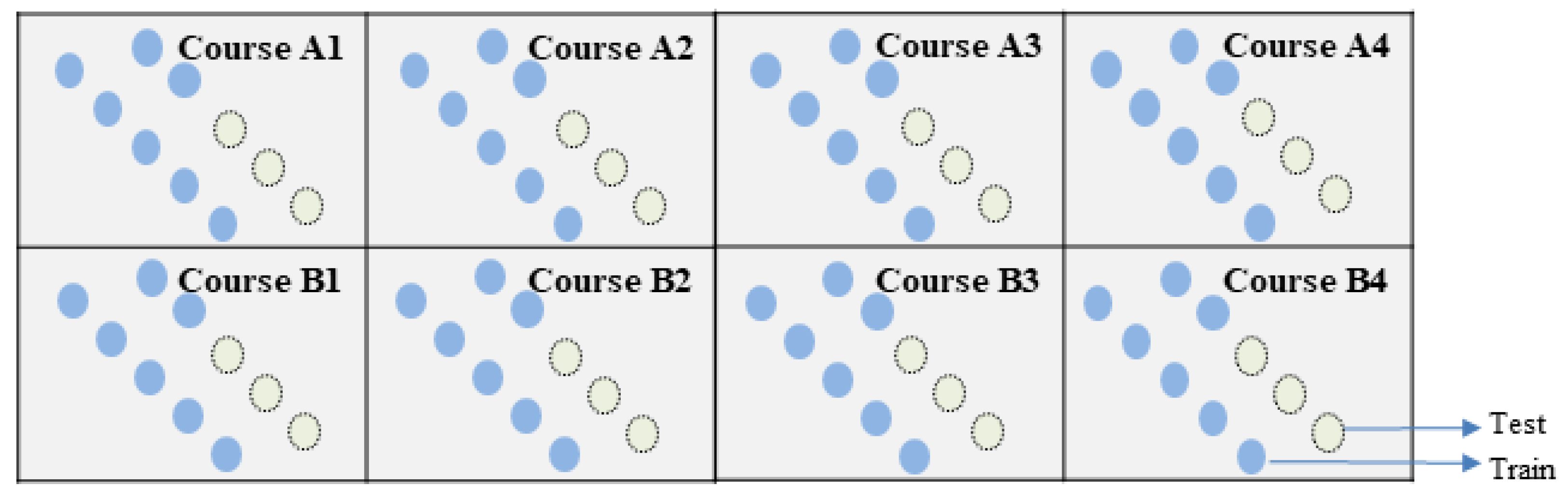
Since educational data are based on courses and semesters, the data have certain relevance within the same course or semester. Therefore, after splitting the training data and test data according to the 80% and 20% ratio, the training and test data will still be correlated (Figure 3). In other words, training and test data may come from the same course or semester [3,9,10,11]. This phenomenon will not happen in reality, although the prediction accuracy will be slightly higher. In reality, it is impossible to train the data of one course and then predict the result itself or to train the data of one semester and then predict the result of the same semester. Because predictions are time-based, training can only be performed on previous data, and future results can be forecasted. These sections were slightly improved in this study.
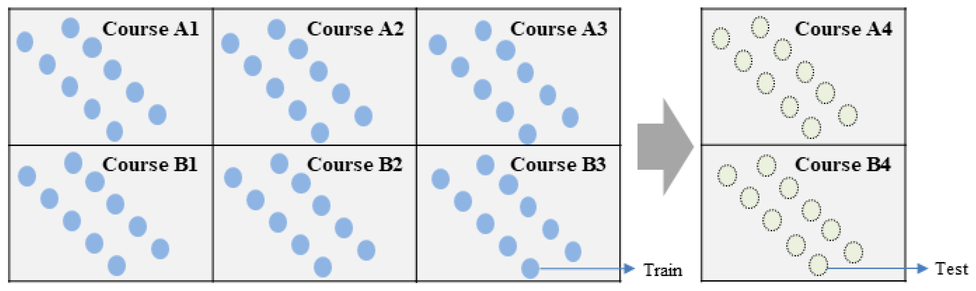
Prediction experiments were conducted by considering the time series of the LMS data. The data from previous semesters were used for training, while the subsequent semester’s data were used for testing. In this work, training data must come from the prior semesters of the test data (Figure 4). Data from four semesters are available in the OULAD. The last semester is the test semester.
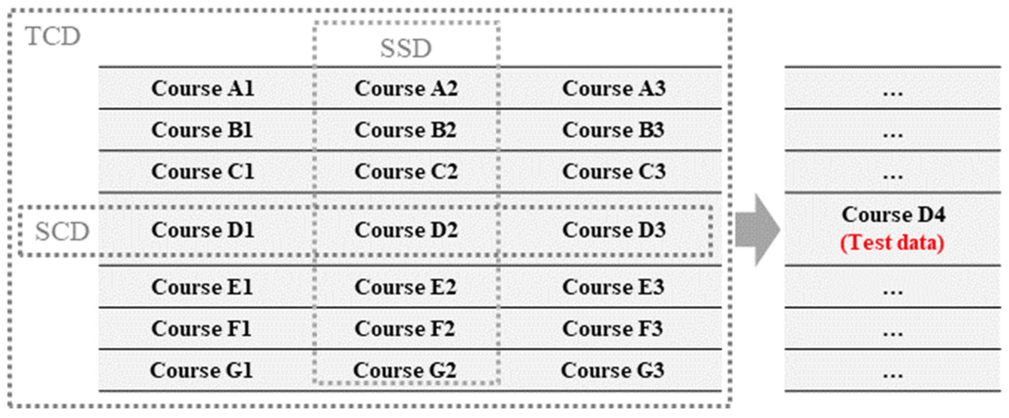
In previous semesters’ data, which data should be utilised for learning? In this regard, we distinguished between three types of training data. The first uses the total course data of all the previous semesters, called TCD; the second uses the same course data from all the previous semesters, called SCD; and the third uses data from a particular previous semester with the same semester code, called SSD.
Three kinds of training data schemes are presented in Table 4 and Figure 5. For example, suppose data from the course AAA in the 2014J semester are used for testing. In this case, TCD contains all the courses in the first three semesters, and SCD includes data for the same courses with 2014J–AAA. Only AAA course data from the first three semesters were used. SSD contains only the same semester code data as all the courses in the 2013J semester.
In this study, the previous semester was not considered the nearest previous semester (refer to Table 4 and Figure 5). The nearest previous semester was not used for prediction because the number of weeks in semester B and semester J differed slightly. In the OULAD, the average number of weeks in the data with semester code B is 34, while in the data with semester code J, the average number of weeks is 38, which is a large discrepancy.
The SCD method aims to check if the prediction accuracy can be improved by studying the same course data. The SSD method was used for testing because different semesters sometimes have different characteristics, such as different lengths and content. TCD is the default mode for comparison.
3.3. Time Points for the Prediction
Since the Open University is a distance-learning university, the school’s semester system differs from that of a regular four-year university. According to the official OULAD data download page, 2013B represents the semester that started in February 2013, and 2013J represents the semester that started in October 2013 [36]. A simple descriptive statistic shows that the average number of weeks across semesters in the OULAD data is approximately 36 weeks. The longest semester is 38 weeks, and the shortest semester is 33 weeks. Therefore, to ensure the fairness of the experiment, the last observation time point was set to 32 weeks.
Although prediction is required every week in a real-world environment, examining all the weeks is too complicated. Thus, in this study, four time points were selected for the prediction as follows: the prediction at the beginning of the semester was calculated according to the 8th week; the middle of the semester was calculated according to the 16th week; the second half of the semester was calculated according to the 24th week; and the end of the semester was calculated according to the 32nd week. Because forecasting aims to predict future possibilities, predictions before the second half of the semester are more critical and have more practical value than those at the end of the semester. The same experiment was conducted at these four time points (see Figure 6).
3.4. Algorithms
Based on previous research [3,5,16], this study tested the prediction results of eight single and three voting algorithms. The eight algorithms included the gradient boosting (GB), bagging, XGBoost, AdaBoost, random forest (RF), logistic regression (LR), support vector machine (SVM), and K-nearest neighbour (KNN) algorithms.
This study also used three types of voting classifiers: Vote-3, Vote-5, and Vote-8. Among these three types, Vote-3 votes on the three basic algorithms: LR, SVM, and KNN. Vote-5 votes on five newer algorithms: XGB, RF, bagging, AdaBoost, and GB. Vote-8 combines Vote-3 and Vote-5, which together vote on eight algorithms (Table 5). The enhancement of the prediction accuracy attributed to the voting methods can be evaluated compared to a single algorithm. The code used in the research has also been shared on GitHub [37].
3.5. Variables
The variables used in our prediction model were as follows [36]. Demographic data are the basic information of learners, and VLE data are the recorded dates for learners to visit, click, and learn in the LMS system. The original data are based on the date, recording the user’s activity at each login. In consideration of prior studies, the main parameters used in the model were chosen after data processing [3,5,16]. There are 20 VLE activity types recorded in the dataset. The cumulative number of clicks for each activity type, the number of visits for each activity type, and the number of days visited were calculated at each time point. The variables are presented in Table 6.
3.6. Evaluation
This study used the F1 score, area under the ROC curve (AUC), and accuracy (ACC) to test the prediction accuracy [38,39]. These evaluations are based on the confusion matrix, a commonly used machine-learning evaluation criterion. The confusion matrix is a table used in classification tasks to summarise the performance of a machine-learning model. It provides a detailed breakdown of the model’s predictions, showing how many instances of each class were correctly or incorrectly predicted (see Figure 7) [40].
- ▪
- True Negative (TN): The number of instances that were actually negative and were correctly predicted as negative.
- ▪
- False Positive (FP): The number of instances that were actually negative but were incorrectly predicted as positive.
- ▪
- False Negative (FN): The number of instances that were actually positive but were incorrectly predicted as negative.
- ▪
- True Positive (TP): The number of instances that were actually positive and were correctly predicted as positive.
The F1 score is the harmonic mean of precision and recall. Accuracy represents the proportion of correctly classified samples out of the total samples. AUC measures the area under the ROC curve, which represents the trade-off between the true positive rate (TPR or recall) and the false positive rate (FPR) [39].
3.7. Explanation with SHAP
SHAP was employed to interpret the model, providing insights into the basis for the model’s predictions [27]. Previous studies using the SHAP algorithm mainly explained the model from an individual instances (local) perspective in the form of a force plot or the important predictor variables of the whole model (global) perspective in the form of a summary plot [30,32,33]. This explanation applies to a single model but is less applicable when comparing two or more models.
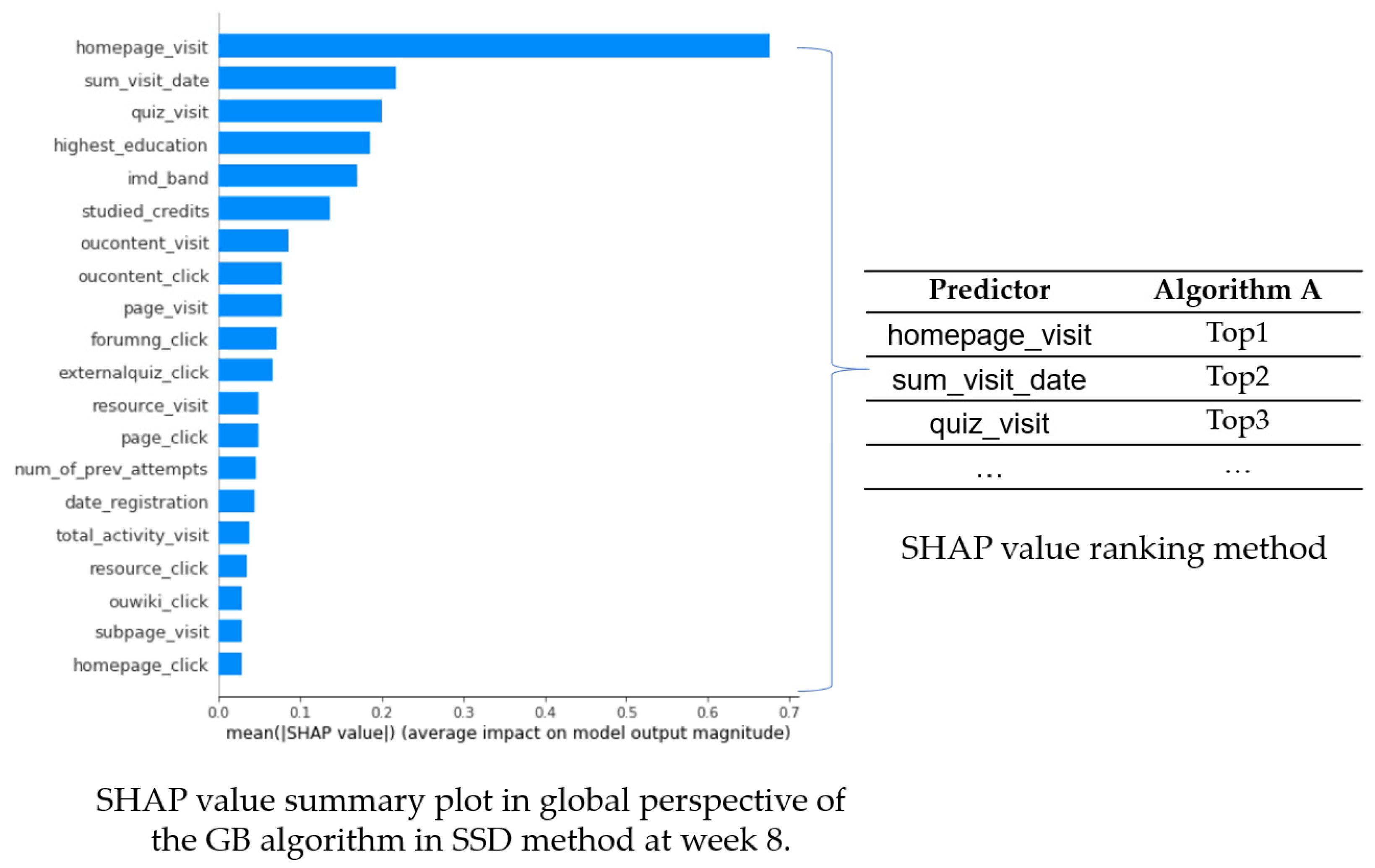
This study used the average of the absolute SHAP values, which is used in the summary_plot, and ranked the average values to compare the differences in predictors between two or more algorithms (Figure 8).
4. Experiment
4.1. Prediction Results
The experiments were conducted following the research design outlined in Figure 2. The experiments were performed on high-performance computers equipped with 20 ft GPUs. The prediction results of each algorithm are presented in Table 7. In this table, the F1 scores of each algorithm are shown. Furthermore, an investigation into the AUC revealed a pattern similar to that observed for the F1 score.
The results indicate the following:
- (1)
- The prediction accuracy gradually increased as the number of weeks increased. As more weekly data were used, the closer the training data was to the final exam, and the better it reflected student learning. So, the prediction accuracy was highest for week 32.
- (2)
- The algorithm with the highest prediction accuracy across the weekly time points was GB in week 8 (0.759); GB was the same as Vote-5 and Vote-8 in week 16 (0.788); and the best prediction was from Vote-5 in week 24 (0.812) and week 32 (0.84).
- (3)
- With the average value calculated in the last line among the three data split methods, the prediction accuracy of SSD was the highest at each time point. As seen in Table 7, the best-performing algorithms at each time point was SSD.
SSD had a higher F1 score than TCD and SCD at all four prediction time points. The result was very positive because SSD only used the data for the same semester code, the training data were reduced, the calculation speed of the model was accelerated, and the lighter prediction model was helpful for practical applications. An explanation of its high accuracy is that semester lengths may differ when the semester code is different; for example, the average number of weeks in semester B is 34, while the average number of weeks in semester J is 38. For the same time point, 32 weeks in semester B represents two weeks left until the end of the lifting period, while in semester J, it represents six weeks left until the end. If the TCD or SCD method was used, the data from semester B were used to predict semester J, increasing the prediction error. Therefore, when using the data for the same semester code for training, the activity data, such as VLE clicks and visits, were more regular and in the same pattern. Since the training data of the SSD method had the same semester length as the test data, the model learning was more targeted. SCD’s prediction accuracy was far from our expectations. The reason for its low accuracy may be an insufficient training sample size. TCD took twenty-one courses, SSD took seven, and SCD only took three.
Table 7 shows the average prediction accuracy of seven courses from AAA to GGG at each time point. To specify the results in more detail, the prediction accuracies of the GB algorithm with Vote-5 in week 24 are listed in Table 8 for each course, as divided into three evaluation criteria, F1, AUC, and ACC, for presentation. Table 8 shows that in week 24, the prediction accuracy of Vote-5 outperformed that of the GB algorithm in the three main evaluation metrics.
LR had a very high prediction accuracy in week 24 (Table 7). Although LR could achieve a prediction accuracy of 0.829 in week 24 when using the TCD method, LR’s accuracy using the TCD method was relatively low in other weeks. The higher prediction accuracy of LR using TCD, which occurred only once, did not prove the prediction stability of LR.
In predicting students at risk of dropping out, to prevent the occurrence of at-risk students and detect and intervene as soon as possible, the prediction in the first half-semester is more important than in the second half-semester. The results show that GB yielded more accurate predictions in the first half-semester, whereas the Vote algorithm yielded better predictions in the second half-semester.
4.2. Interpretation Using XAI
Further examination of the prediction details for each course was conducted to understand why the prediction accuracy of the Vote-5 algorithm was lower than that of the GB algorithm in the eighth week. The SHAP algorithm was employed to compare the primary variables used in the prediction process.
First, Table 7 shows that XGB had the lowest result among the prediction results for week 8. XGB was included in Vote-5 due to its strong prediction performance in the second half of the semester and its favourable performance in earlier studies [16]. The prediction performance of the XGB and GB algorithms in each of the seven courses in week 8 was compared in detail. Additional details of the experiment led to the conclusion that the prediction accuracy of XGB was lower than that of GB, especially in the DDD and GGG courses. Table 9 provides a detailed comparison of these two courses. The two algorithms differ significantly regarding the main predictor variables used.
The sorting shown in Table 9 was performed according to the average of the absolute values of the SHAP value for each variable. The results show that the order of main variables used differed between the two algorithms. In previous studies, researchers used SHAP to explain more in the form of graphs or plots [30,32]. However, comparing and explaining more than two models using graphs is difficult. The primary variable differs between multiple models.
For week 8, in all seven courses, the variable SHAP value ranking table of the GB algorithm is presented in Table 10. Although the order of the main variables used by GB in the seven courses differed, the TOP 3 variables mainly focused on homepage_visit, external quiz_click, quiz_visit, sum_visit_date, highest_education, and studied_credits. Here, studied_credits is the total number of credits for the modules the student is studying.
5. Conclusion and Discussion
This study conducted at-risk prediction experiments that reflect reality more closely than similar experiments in previous studies [3,5]. This study viewed the at-risk prediction results on a per-course basis and used data from previous semesters to predict the current semester. Four prediction time points were selected, and the model was trained using three different training data schemes. Eight single and three voting algorithms were selected.
The experiments revealed that different algorithms performed differently for various courses and time points. After the 16th week, the prediction accuracy using the Vote-5 algorithm was higher than that using the single GB algorithm. In the 8th week, the effect of Vote-5 was absent due to the lower data accumulation. The model used in this study achieved a prediction accuracy of 0.759, 0.788, 0.812, and 0.84 at four representative time points, i.e., week 8, week 16, week 24, and week 32, respectively.
When choosing the training data for the model, the SSD method performed best with OULAD data, followed by TCD and, finally, SCD. Training data must be selected according to the characteristics of the data. Our experiments demonstrated that the prediction accuracy could be improved by choosing the relevant training data closest to the test data, even when a relatively small dataset was used for learning. With OULAD data, using the same semester code method saved time and improved the prediction accuracy. Experiments performed on other data should select the training data according to the specific characteristics of each dataset. Consequently, we developed and tested a model using SSD data for training and GB and Vote-5 for prediction.
SHAP was employed to perform a comparative analysis of the primary variables utilised in the prediction model. Previous research mostly listed the SHAP value chart of a particular model; the current study is innovative in that it compared the variable ranking of the two models [30,32]. Examining the order of the primary predictors used by the model allows for a deeper understanding of the basis for the model by providing insights into the distinct prediction methods of various algorithms. This approach will help teachers understand at-risk students more.
Universities can use the machine-learning-based prediction model proposed in this study to measure student dropout risk in real time and alert teachers. This study confirmed that accurately predicting dropout rates using students’ online learning behaviours is feasible. Furthermore, informing teachers that the number of homepage visits, quiz visits, cumulative days visited, total credits taken, and the multiple deprivation index (IMD) band of the student’s residence are the main predictors of dropout rates will encourage them to pay more attention to these features.
Moreover, this study found that the relative prediction accuracy of the algorithms could differ between the first half of a semester and the second half of a semester. This finding suggests that the best method for predicting the dropout rate may differ between the first and second half of the semester. This study did not explore the specific reasons for this difference, although teachers can be mindful of it in their practice.
This study has some limitations. First, the variables of the assessment scores were not included in the model, which will be considered in future research. Second, the data used in this study are somewhat dated; more in-depth studies using more recent data from during the COVID-19 pandemic are planned. The integrated model in this study did not show a higher prediction effect at the eighth week; future research should explore a model with better prediction accuracy at all time points. In this study, SHAP was only used to explain the model for week 8; future studies should attempt to explain more models at other time points, including the voting model. In addition, the results based on SHAP can be analysed by comparing the characteristics of data from each course.
Author Contributions
Conceptualisation, C.Z. and H.A.; methodology, C.Z.; software, C.Z.; validation, C.Z.; formal analysis, C.Z.; investigation, C.Z.; resources, C.Z.; data curation, C.Z.; writing—original draft preparation, C.Z.; writing—review and editing, C.Z. and H.A.; visualisation, C.Z.; supervision, C.Z. and H.A.; project administration, C.Z. All authors have read and agreed to the published version of the manuscript.
Funding
This research received no external funding.
Institutional Review Board Statement
Not applicable.
Informed Consent Statement
Not applicable.
Data Availability Statement
The dataset used in the current study is available at https://analyse.kmi.open.ac.uk/open_dataset. The Python code used in this study is available at https://github.com/githubthank/At-Risk_Prediction.
Conflicts of Interest
The authors declare no conflict of interest.
References
- Kuzilek, J.; Hlosta, M.; Zdrahal, Z. Open university learning analytics dataset. Sci. Data 2017, 4, 1–8. [Google Scholar] [CrossRef] [PubMed]
- Feng, W.; Tang, J.; Liu, T.X. Understanding dropouts in MOOCs. Proc. AAAI Conf. Artif. Intell. 2019, 33, 517–524. [Google Scholar] [CrossRef]
- Kuzilek, J.; Hlosta, M.; Herrmannova, D.; Zdrahal, Z.; Vaclavek, J.; Wolff, A. OU Analyse: Analysing at-risk students at The Open University. Learn. Anal. Rev. 2015, LAK15-1, 1–6. [Google Scholar]
- Alshabandar, R.; Hussain, A.; Keight, R.; Laws, A.; Baker, T. The application of Gaussian mixture models for the identification of at-risk learners in massive open online courses. In Proceedings of the 2018 IEEE Congress on Evolutionary Computation (CEC), Rio de Janeiro, Brazil, 8–13 July 2018; pp. 1–8. [Google Scholar]
- Hlosta, M.; Zdrahal, Z.; Zendulka, J. Ouroboros: Early identification of at-risk students without models based on legacy data. In Proceedings of the Seventh International Learning Analytics & Knowledge Conference, Vancouver, BC, Canada, 13–17 March 2017; pp. 6–15. [Google Scholar]
- Lykourentzou, I.; Giannoukos, I.; Nikolopoulos, V.; Mpardis, G.; Loumos, V. Dropout prediction in e-learning courses through the combination of machine learning techniques. Comput. Educ. 2009, 53, 950–965. [Google Scholar] [CrossRef]
- Chaplot, D.S.; Rhim, E.; Kim, J. Predicting student attrition in MOOCs using sentiment analysis and neural networks. In Proceedings of the Workshop at the 17th International Conference on Artificial Intelligence in Education (AIED-WS 2015), Madrid, Spain, 22–26 June 2015; pp. 7–12. [Google Scholar]
- Liang, J.; Li, C.; Zheng, L. Machine learning application in MOOCs: Dropout prediction. In Proceedings of the 2016 11th International Conference on Computer Science & Education (ICCSE), Nagoya, Japan, 23–25 August 2016; pp. 52–57. [Google Scholar]
- Cobos, R.; Wilde, A.; Zaluska, E. Predicting attrition from massive open online courses in FutureLearn and edX. In Proceedings of the 7th International Learning Analytics and Knowledge Conference, Vancouver, BC, Canada, 13–17 March 2017. [Google Scholar]
- Yukselturk, E.; Ozekes, S.; Turel, Y.K. Predicting dropout student: An application of data mining methods in an online education program. Eur. J. Open Distance e-Learn. 2014, 17, 118–133. [Google Scholar] [CrossRef]
- Queiroga, E.M.; Lopes, J.L.; Kappel, K.; Aguiar, M.; Araújo, R.M.; Munoz, R.; Villarroel, R.; Cechinel, C. A learning analytics approach to identify students at risk of dropout: A case study with a technical distance education course. Appl. Sci. 2020, 10, 3998. [Google Scholar] [CrossRef]
- Mubarak, A.A.; Cao, H.; Zhang, W. Prediction of students’ early dropout based on their interaction logs in online learning environment. Interact. Learn. Environ. 2022, 30, 1414–1433. [Google Scholar] [CrossRef]
- Haiyang, L.; Wang, Z.; Benachour, P.; Tubman, P. A time series classification method for behaviour-based dropout prediction. In Proceedings of the 2018 IEEE 18th International Conference on Advanced Learning Technologies (ICALT), Mumbai, India, 9–13 July 2018; pp. 191–195. [Google Scholar]
- Zhou, Y.; Zhao, J.; Zhang, J. Prediction of learners’ dropout in E-learning based on the unusual behaviors. Interact. Learn. Environ. 2020, 31, 1–25. [Google Scholar] [CrossRef]
- Abd El-Rady, A. An ontological model to predict dropout students using machine learning techniques. In Proceedings of the 2020 3rd International Conference on Computer Applications & Information Security (ICCAIS), Riyadh, Saudi Arabia, 19–21 March 2020; IEEE: New York, NY, USA; pp. 1–5. [Google Scholar]
- Jha, N.I.; Ghergulescu, I.; Moldovan, A.N. OULAD MOOC dropout and result prediction using ensemble, deep learning and regression techniques. In Proceedings of the 11th International Conference on Computer Supported Education (CSEDU 2019), Crete, Greece, 2–4 May 2019; pp. 154–164. [Google Scholar]
- Tan, M.; Shao, P. Prediction of student dropout in e-Learning program through the use of machine learning method. Int. J. Emerg. Technol. Learn. 2015, 10, 11–17. [Google Scholar] [CrossRef]
- Batool, S.; Rashid, J.; Nisar, M.W.; Kim, J.; Mahmood, T.; Hussain, A. A random forest students’ performance prediction (rfspp) model based on students’ demographic features. In Proceedings of the 2021 Mohammad Ali Jinnah University International Conference on Computing (MAJICC), Karachi, Pakistan, 15–17 July 2021; pp. 1–4. [Google Scholar]
- Kittler, J.; Hatef, M.; Duin, R.P.; Matas, J. On combining classifiers. IEEE Trans. Pattern Anal. Mach. Intell. 1998, 20, 226–239. [Google Scholar] [CrossRef]
- Kizilcec, R.F.; Piech, C.; Schneider, E. Deconstructing disengagement: Analyzing learner subpopulations in massive open online courses. In Proceedings of the Third International Conference on Learning Analytics and Knowledge, Leuven, Belgium, 8–13 April 2013; pp. 170–179. [Google Scholar]
- Aldowah, H.; Al-Samarraie, H.; Alzahrani, A.I.; Alalwan, N. Factors affecting student dropout in MOOCs: A cause and effect decision-making model. J. Comput. High. Educ. 2020, 32, 429–454. [Google Scholar] [CrossRef]
- Coussement, K.; Phan, M.; De Caigny, A.; Benoit, D.F.; Raes, A. Predicting student dropout in subscription-based online learning environments: The beneficial impact of the logit leaf model. Decis. Support Syst. 2020, 135, 113325. [Google Scholar] [CrossRef]
- Dewan MA, A.; Lin, F.; Wen, D. Predicting dropout-prone students in e-learning education system. In Proceedings of the 2015 IEEE 12th International Conference on Ubiquitous Intelligence and Computing and 2015 IEEE 12th International Conference on Autonomic and Trusted Computing and 2015 IEEE 15th International Conference on Scalable Computing and Communications and Its Associated Workshops (UIC-ATC-ScalCom), Beijing, China, 10–14 August 2015; pp. 1735–1740. [Google Scholar]
- da Silva, P.M.; Lima, M.N.; Soares, W.L.; Silva, I.R.; de Fagundes, R.A.; de Souza, F.F. Ensemble regression models applied to dropout in higher education. In Proceedings of the 2019 8th Brazilian Conference on Intelligent Systems (BRACIS), Salvador, Brazil, 15–18 October 2019; pp. 120–125. [Google Scholar]
- Patacsil, F.F. Survival analysis approach for early prediction of student dropout using enrollment student data and ensemble models. Univers. J. Educ. Res. 2020, 8, 4036–4047. [Google Scholar] [CrossRef]
- Ribeiro, M.T.; Singh, S.; Guestrin, C. “Why should I trust you?” Explaining the predictions of any classifier. In Proceedings of the 22nd ACM SIGKDD International Conference on Knowledge Discovery and Data Mining, San Francisco, CA, USA, 13–17 August 2016; pp. 1135–1144. [Google Scholar]
- Lundberg, S.M.; Lee, S.I. Consistent feature attribution for tree ensembles. arXiv 2017, arXiv:1706.06060. [Google Scholar]
- Bach, S.; Binder, A.; Montavon, G.; Klauschen, F.; Müller, K.R.; Samek, W. On pixel-wise explanations for non-linear classifier decisions by layer-wise relevance propagation. PLoS ONE 2015, 10, e0130140. [Google Scholar] [CrossRef] [PubMed]
- Selvaraju, R.R.; Cogswell, M.; Das, A.; Vedantam, R.; Parikh, D.; Batra, D. Grad-cam: Visual explanations from deep networks via gradient-based localization. In Proceedings of the IEEE International Conference on Computer Vision, Venice, Italy, 22–29 October 2017; pp. 618–626. [Google Scholar]
- Alwarthan, S.; Aslam, N.; Khan, I.U. An explainable model for identifying at-risk student at higher education. IEEE Access 2022, 10, 107649–107668. [Google Scholar] [CrossRef]
- Smith, B.I.; Chimedza, C.; Bührmann, J.H. Individualized help for at-risk students using model-agnostic and counterfactual explanations. Educ. Inf. Technol. 2022, 27, 1539–1558. [Google Scholar] [CrossRef]
- Dass, S.; Gary, K.; Cunningham, J. Predicting student dropout in self-paced MOOC course using random forest model. Information 2021, 12, 476. [Google Scholar] [CrossRef]
- Baranyi, M.; Nagy, M.; Molontay, R. Interpretable deep learning for university dropout prediction. In Proceedings of the 21st Annual Conference on Information Technology Education, Virtual Event, USA, 7–9 October 2020; pp. 13–19. [Google Scholar]
- Albreiki, B. Framework for automatically suggesting remedial actions to help students at risk based on explainable ML and rule-based models. Int. J. Educ. Technol. High. Educ. 2022, 19, 1–26. [Google Scholar] [CrossRef]
- Alonso, J.M.; Casalino, G. Explainable artificial intelligence for human-centric data analysis in virtual learning environments. In International Workshop on Higher Education Learning Methodologies and Technologies Online; Springer: Cham, Switzerland, 2019; pp. 125–138. [Google Scholar]
- OULAD Dataset Link. Available online: https://analyse.kmi.open.ac.uk/open_dataset (accessed on 12 November 2023).
- Github Code Link. Available online: https://github.com/githubthank/At-Risk_Prediction (accessed on 12 November 2023).
- Sasaki, Y. The truth of the F-measure. Teach Tutor Mater 2007, 1, 1–5. [Google Scholar]
- Fawcett, T. An introduction to ROC analysis. Pattern Recognit. Lett. 2006, 27, 861–874. [Google Scholar] [CrossRef]
- Powers, D.M. Evaluation: From precision, recall and F-measure to ROC, informedness, markedness and correlation. J. Mach. Learn. Technol. 2011, 2, 37–63. [Google Scholar]
Figure 1.
Voting classifier algorithm.

Figure 2.
Research framework.

Figure 3.
Data split method of previous research.

Figure 4.
Data split method in this study.

Figure 5.
Three kinds of training data schemes.

Figure 6.
Prediction time points.

Figure 7.
Confusion matrix and the formula of the accuracy and F1 score.

Figure 8.
SHAP value ranking method.


Table 1.
At-risk prediction in e-learning.
| Citation | Dataset | Algorithms |
|---|---|---|
| Lykourentzou et al. [6] | The National Technical University of Athens | FFNN, SVM, PESFAM |
| Yukselturk et al. [10] | Government University in the capital city of Turkey | KNN, DT, NB, ANN, |
| Chaplot et al. [7] | Coursera | NN, SA |
| Kuzilek et al. [3] | The Open University (UK) | KNN, CART, NB, Voting |
| Tan and Shao [17] | Open University of China | DT, BN, ANN |
| Cobos et al. [9] | EdX | GBM, KNN, LR, XGB |
| Hlosta et al. [5] | The Open University (UK) | LR, SVM, RF, NB, XGB |
| Haiyang et al. [13] | The Open University (UK) | TSF |
| Alshabandar et al. [4] | The Open University (UK) | EDDA |
| Jha et al. [16] | The Open University (UK) | GB, DRF, DL, GLM |
| Queiroga et al. [11] | Instituto Federal Sul Rio-Grandense (IFSul) in Brazil | GA, AdaBoost, DT, LR, MLP, RF |
| Zhou et al. [14] | E-learning big data technology company in China | Cox proportional hazard model |
| Mubarak et al. [12] | The Open University (UK) | SELOR, IOHMM, LR, SVM, DT, RF |
Table 2.
At-risk prediction in e-learning using ensemble algorithms.
| Citation | Dataset | Algorithms |
|---|---|---|
| Dewan et al. [23] | Simulation data | Vote (KNN, RBF, SVM) |
| Kuzilek et al. [3] | The Open University (UK) | Vote (KNN, CART, NB) |
| da Silva et al. [24] | National Institute of Educational Studies and Research (INEP) in the year 2013, Brazil | Ensemble (bagging + LR, robust regression, ridge regression), lasso regression, boosting, RF, support vector regression, KNN |
| Patacsil [25] | Pangasinan State University Urdaneta City Campus | DT, forest tree, J-48, ensemble model (bagging + DT, bagging + forest tree, bagging + J-48), AdaBoost + DT, AdaBoost + forest tree, AdaBoost + J-48 |
Table 3.
At-risk prediction in e-learning using eXplainable AI.
| Citation | Dataset | Algorithms |
|---|---|---|
| Alonso et al. [35] | The Open University (UK) | J48, RepTree, random tree, FURIA (+ ExpliClas) |
| Baranyi [33] | Budapest University of Technology and Economics | FCNN, TabNet, XGB, RF, bagging (+ SHAP) |
| Dass [32] | Math course College Algebra and Open edX offered by EdPlus at Arizona State University | RF (+ SHAP) |
| Alwarthan et al. [30] | The preparatory year students from the humanities track at Imam Abdulrahman Bin Faisal University (SMOTE) | RF, ANN, SVM (+ LIME, + SHAP) |
| Albreiki [34] | United Arab Emirates University (UAEU) | XGB, LightGBM, SVM, GaussianNB, ExtraTrees, bagging, RF, MLP (+ LIME) |
Table 4.
Three kinds of training data schemes.
| Semester 2013-B | Semester 2013-J | Semester 2014-B | Semester 2014-J | |
| Course AAA | (TCD) | (TCD) | (TCD) | (Test data) |
| Course GGG | (TCD) | (TCD) | (TCD) | |
| Semester 2013-B | Semester 2013-J | Semester 2014-B | Semester 2014-J | |
| Course AAA | (SCD) | (SCD) | (SCD) | (Test data) |
| Course GGG | ||||
| Semester 2013-B | Semester 2013-J | Semester 2014-B | Semester 2014-J | |
| Course AAA | (SSD) | (Test data) | ||
| Course GGG | (SSD) | |||
Table 5.
Table of algorithms.
| Algorithm | GB | Bagging | XGB | AdaBoost | RF | LR | SVM | KNN |
| Vote-5 (XGB, RF, bagging, AdaBoost, GB) | Vote-3 (LR, SVM, KNN) | |||||||
| Vote-8 (LR, SVM, KNN, XGB, RF, bagging, AdaBoost, GB) | ||||||||
Table 6.
Experiment variables.
| Type | Variable |
|---|---|
| Demographic data (independent variables) | Studied_Credits |
| Number_of_Previous_Attempts | |
| Highest_Education | |
| IMD_Band | |
| Age_Band | |
| Gender | |
| Region | |
| Disability | |
| Date_registration | |
| VLE activity data (independent variables) | The number of clicks for each 20 VLE activity variables |
| The number of visits for each 20 VLE activity variables | |
| The number of clicks for all the VLE activity variables | |
| The number of visits for all the VLE activity variables | |
| The number of visit days | |
| Dependent variable | Final_result |
Table 7.
F1 scores using different experiment methods.
| Algorithm | Week 8 (F1) | Week 16 (F1) | Week 24 (F1) | Week 32 (F1) | ||||||||
|---|---|---|---|---|---|---|---|---|---|---|---|---|
| TCD | SCD | SSD | TCD | SCD | SSD | TCD | SCD | SSD | TCD | SCD | SSD | |
| LR | 0.732 | 0.702 | 0.742 | 0.754 | 0.745 | 0.776 | 0.829 | 0.777 | 0.774 | 0.802 | 0.841 | 0.807 |
| SVM | 0.688 | 0.730 | 0.728 | 0.743 | 0.752 | 0.766 | 0.781 | 0.794 | 0.798 | 0.817 | 0.831 | 0.825 |
| KNN | 0.690 | 0.733 | 0.723 | 0.737 | 0.750 | 0.750 | 0.772 | 0.803 | 0.767 | 0.806 | 0.833 | 0.806 |
| XGB | 0.706 | 0.685 | 0.709 | 0.769 | 0.758 | 0.768 | 0.780 | 0.779 | 0.797 | 0.817 | 0.832 | 0.835 |
| RF | 0.712 | 0.682 | 0.738 | 0.770 | 0.750 | 0.785 | 0.796 | 0.777 | 0.809 | 0.820 | 0.821 | 0.839 |
| Bagging | 0.712 | 0.643 | 0.741 | 0.765 | 0.756 | 0.780 | 0.781 | 0.733 | 0.803 | 0.821 | 0.816 | 0.839 |
| AdaBoost | 0.722 | 0.666 | 0.745 | 0.761 | 0.748 | 0.767 | 0.757 | 0.784 | 0.781 | 0.778 | 0.781 | 0.819 |
| GB | 0.733 | 0.658 | 0.759 | 0.782 | 0.749 | 0.788 | 0.793 | 0.771 | 0.798 | 0.808 | 0.797 | 0.836 |
| Vote-3 | 0.720 | 0.735 | 0.745 | 0.760 | 0.775 | 0.779 | 0.793 | 0.805 | 0.800 | 0.824 | 0.838 | 0.830 |
| Vote-5 | 0.724 | 0.675 | 0.745 | 0.783 | 0.760 | 0.788 | 0.797 | 0.787 | 0.812 | 0.824 | 0.833 | 0.840 |
| Vote-8 | 0.719 | 0.674 | 0.747 | 0.776 | 0.756 | 0.788 | 0.788 | 0.787 | 0.803 | 0.814 | 0.828 | 0.837 |
| Average | 0.714 | 0.689 | 0.738 | 0.764 | 0.754 | 0.776 | 0.788 | 0.782 | 0.795 | 0.812 | 0.823 | 0.828 |
Note: Bolded values show the best performance for each period. F1 means F1 Score, the harmonic mean of precision and recall. TCD means prediction using the total course data from all previous semesters. SCD means prediction using only data from the same course in all previous semesters. SSD means prediction using only a particular previous semester with the same semester code.
Table 8.
Results of predictions using the same semester code data (SSD) in the 24th week.
| Course | Gradient Boosting (GB) | Vote-5 | ||||
|---|---|---|---|---|---|---|
| F1 | AUC | ACC | F1 | AUC | ACC | |
| AAA | 0.817 | 0.697 | 0.745 | 0.846 | 0.701 | 0.775 |
| BBB | 0.733 | 0.766 | 0.765 | 0.765 | 0.783 | 0.782 |
| CCC | 0.744 | 0.77 | 0.74 | 0.744 | 0.77 | 0.739 |
| DDD | 0.696 | 0.747 | 0.763 | 0.705 | 0.754 | 0.77 |
| EEE | 0.9 | 0.862 | 0.877 | 0.908 | 0.875 | 0.888 |
| FFF | 0.849 | 0.85 | 0.847 | 0.866 | 0.866 | 0.862 |
| GGG | 0.844 | 0.816 | 0.818 | 0.85 | 0.814 | 0.821 |
| Avg | 0.798 | 0.787 | 0.794 | 0.812 | 0.795 | 0.805 |
Note: Bolded values show the best performance for each course. F1 means F1 Score, the harmonic mean of precision and recall. AUC means the area under the ROC curve. ACC means the accuracy of correctly classified.
Table 9.
SHAP value ranking table of XGB and GB using the SSD method at week 8.
| Feature | Course DDD | Course GGG | ||
|---|---|---|---|---|
| XGBoost | GB | XGBoost | GB | |
| homepage_visit | Top 1 | Top 1 | Top 1 | Top 2 |
| external_quiz_click | Top 2 | Top 2 | Top 10 | |
| quiz_visit | Top 7 | Top 3 | Top 6 | |
| sum_visit_date | Top 4 | Top 4 | Top 6 | Top 4 |
| highest_education | Top 6 | Top 5 | Top 3 | Top 3 |
| studied_credits | Top 5 | Top 6 | Top 2 | Top 1 |
| imd_band | Top 9 | Top 7 | Top 5 | Top 5 |
| ouwiki_click | Top 8 | Top 8 | ||
| forumng_click | Top 9 | |||
| resource_visit | Top 10 | Top 8 | ||
| page_visit | Top 9 | |||
| resource_click | Top 7 | |||
| oucontent_click | Top 10 | |||
| date_registration | Top 7 | |||
| homepage_click | Top 3 | Top 4 | ||
| total_activity_click | Top 10 | Top 8 | ||
Table 10.
SHAP value ranking table for the GB algorithm using the SSD method at week 8.
| Feature | AAA | BBB | CCC | DDD | EEE | FFF | GGG |
|---|---|---|---|---|---|---|---|
| homepage_visit | Top 1 | Top 1 | Top 1 | Top 1 | Top 1 | Top 1 | Top 2 |
| external_quiz_click | Top 10 | Top 2 | Top 10 | Top 10 | |||
| quiz_visit | Top 3 | Top 2 | Top 2 | Top 3 | Top 2 | Top 2 | Top 6 |
| sum_visit_date | Top 2 | Top 4 | Top 5 | Top 4 | Top 5 | Top 3 | Top 4 |
| highest_education | Top 4 | Top 3 | Top 4 | Top 5 | Top 3 | Top 4 | Top 3 |
| studied_credits | Top 6 | Top 5 | Top 3 | Top 6 | Top 4 | Top 5 | Top 1 |
| imd_band | Top 5 | Top 6 | Top 6 | Top 7 | Top 6 | Top 6 | Top 5 |
| ouwiki_click | Top 8 | ||||||
| forumng_click | Top 10 | Top 7 | Top 9 | Top 7 | |||
| resource_visit | Top 8 | Top 9 | Top 10 | Top 7 | Top 8 | ||
| page_visit | Top 9 | Top 9 | Top 8 | Top 9 | Top 8 | Top 9 | |
| resource_click | Top 10 | Top 7 | |||||
| oucontent_click | Top 8 | Top 10 | |||||
| page_click | |||||||
| oucontent_visit | Top 7 | Top 8 | Top 9 | ||||
| quiz_click | Top 7 |
Disclaimer/Publisher’s Note: The statements, opinions and data contained in all publications are solely those of the individual author(s) and contributor(s) and not of MDPI and/or the editor(s). MDPI and/or the editor(s) disclaim responsibility for any injury to people or property resulting from any ideas, methods, instructions or products referred to in the content. |
© 2023 by the authors. Licensee MDPI, Basel, Switzerland. This article is an open access article distributed under the terms and conditions of the Creative Commons Attribution (CC BY) license (https://creativecommons.org/licenses/by/4.0/).
Share and Cite
MDPI and ACS Style
Zhang, C.; Ahn, H. E-Learning at-Risk Group Prediction Considering the Semester and Realistic Factors. Educ. Sci. 2023, 13, 1130. https://0-doi-org.brum.beds.ac.uk/10.3390/educsci13111130
AMA Style
Zhang C, Ahn H. E-Learning at-Risk Group Prediction Considering the Semester and Realistic Factors. Education Sciences. 2023; 13(11):1130. https://0-doi-org.brum.beds.ac.uk/10.3390/educsci13111130
Chicago/Turabian StyleZhang, Chenglong, and Hyunchul Ahn. 2023. "E-Learning at-Risk Group Prediction Considering the Semester and Realistic Factors" Education Sciences 13, no. 11: 1130. https://0-doi-org.brum.beds.ac.uk/10.3390/educsci13111130
Note that from the first issue of 2016, this journal uses article numbers instead of page numbers. See further details here.