
Optimal Sizing of Stand-Alone Microgrids Based on Recent Metaheuristic Algorithms


1
Electrical Engineering Department, Faculty of Engineering, Minia University, Minia 61111, Egypt
2
College of Engineering and Technology, American University of the Middle East, Egaila 54200, Kuwait
3
Nuclear Research Center, Engineering Department, ETRR-2, Atomic Energy Authority (EAEA), Cairo 11787, Egypt
4
Nuclear Research Center, Reactors Department, Egyptian Atomic Energy Authority, Cairo 11787, Egypt
5
Electrical Power Systems Department, Moscow Power Engineering Institute, 111250 Moscow, Russia
*
Authors to whom correspondence should be addressed.
Mathematics 2022, 10(1), 140; https://0-doi-org.brum.beds.ac.uk/10.3390/math10010140
Submission received: 9 December 2021
/
Revised: 27 December 2021
/
Accepted: 27 December 2021
/
Published: 4 January 2022
(This article belongs to the Topic Multi-Energy Systems)
Abstract
:Scientists have been paying more attention to the shortage of water and energy sources all over the world, especially in the Middle East and North Africa (MENA). In this article, a microgrid configuration of a photovoltaic (PV) plant with fuel cell (FC) and battery storage systems has been optimally designed. A real case study in Egypt in Dobaa region of supplying safety loads at a nuclear power plant during emergency cases is considered, where the load characteristics and the location data have been taken into consideration. Recently, many optimization algorithms have been developed by researchers, and these algorithms differ from one another in their performance and effectiveness. On the other hand, there are recent optimization algorithms that were not used to solve the problem of microgrids design in order to evaluate their performance and effectiveness. Optimization algorithms of equilibrium optimizer (EQ), bat optimization (BAT), and black-hole-based optimization (BHB) algorithms have been applied and compared in this paper. The optimization algorithms are individually used to optimize and size the energy systems to minimize the cost. The energy systems have been modeled and evaluated using MATLAB.
1. Introduction
Recently, Egypt has shown interest and determination to be one of the worldwide energy producers. In 2030, Egypt plans to increase its renewable energy production to 30% of its demand to support the rising population and growth [1,2,3]. Egypt’s location provides it with an excellent average irradiance all over the year. In addition, the wind energy atlas shows a great ability to depend on wind energy. In the last decade, the total installed capacity of new and renewable energy sources of wind and solar power plants has been raised from 1157 MW in 2017/2018 to 2247 MW in 2018/2019 with an increase of 94.2%, as reported in the 2018/2019 annual report of the Egyptian electricity holding company [4,5]. Likewise, the total energy generated from wind and solar sources, which are connected to the unified national grid, has been increased from 2871 GWh in 2017/2018 to 4543 GWh in 2018/2019 with a growth rate of 58.2% [1,2,3,4,5,6]; on the other hand, solar energy generation has increased by 184% reaching a value of 1525 GWh in 2019 [1,2,3,4,5,6].
Several renewable energy configurations have been designed and evaluated for such cases. Different configurations that are based on solar, wind, and fuel cells have been introduced [7,8,9]. Solar PV energy is a great source of clean energy in Egypt source; the high average irradiance all over the year [4], as well as the low costs of both operation and maintenance, led to a remarkable increase in the investments in PV plants to be the safest source in distant zones [7,8,9]. PV plants became the main energy source in most of the presented system configurations in Egypt as well as other countries [1,2,3,4,5,6,7,8,9]. Wind energy, storage batteries, geothermal, wave, tidal energies, and fuel cells are other sources that can be used with PV forming a hybrid system. The necessity of hybridization of other energy sources with PV sources is due to the variation in the generated solar energy with many factors such as meteorological conditions. Another suggested case study of a microgrid is to feed the nuclear power plants (NPPs) during emergencies, enhancing the electrical system safety and NPP reliability.
Design of emergency power systems provides electrically independent and physically separated power distribution divisions. One is designated odd and the other even. The distribution design provides power to redundant station loads and prevents failures or damage of one division cascaded to the others. Integration of all power sources in a microgrid arrangement enhances the safety of operation, normal shutdown, and unplanned shutdown, as well as overall plant safety. In addition, it mitigates the negative impact of emergency power absence on the environment. Solar and/or wind energy may supply the services and emergency load, while fuel cells can be used as storage devices.
Backup diesel generators have been used for compensating the lack of solar energy in the shortage periods [10]. However, the dependency on fossil fuels is still the main problem besides environmental conditions [3]. On the other side, batteries storage units are the first decision as a traditional storage component. The battery storage units assist the system to be both stable and reliable. More attention has been paid to reducing the cost of battery units and raising its efficiency and lifetime. Researchers have proposed the usage of battery units to improve the power quality of power systems that are being interconnected with renewable energy sources [7,8,9,10]. Fuel cells have been utilized as a reliable storage device with acceptable efficiency [11]. Fuel cells have distinguished advantages compared to the battery units, which include lower cost and less negative effect on the environment. Water-based FC with a combined electrolyzer unit is the standard type that is used with renewable energy sources. From the reported papers [7,8,9,10,11,12], it could be noted that the battery storage units increase the cost of the COE of all configured systems. Moreover, the grid-connected hybrid systems, in most cases, have the best COE. The reasons may be summarized in the lower cost of kWh obtained from the grid compared to the initial costs obtained from renewable energy sources. However, in recent years, acceptable rate reduction in the initial costs of renewable energy sources increased the chances of using such sources.
Several research studies have been carried to develop a reliable procedure to optimize the configuration of hybrid energy systems. Few reported attempts considered real case studies, while others focused on the techniques and methodologies [12,13,14,15,16,17,18,19,20,21]. Great efforts have been made to better manage the uncertainties of renewable energy systems (RES), cost of energy (COE), and load demands (LD) by various recent research studies. In [22], the authors proposed the management strategy of RES uncertainties, the electricity price, and LD based on a hybrid stochastic/robust (HSR) optimizer in different scenarios, which have the advantage of improving the convergence characteristics. The authors in [23] developed a distributed robust optimization approach to overcome the restrictions of the dispatchable flexible resources taking into account the uncertainties from RES and LD based on different constraints that can be appropriate in piratical schemes with tacking the transmission loss in the consideration.
In 2020 [12], a hybrid configuration composed of PV plant, WT plant, battery units, and diesel generators was designed, involving a comprehensive comparison between the different possible configurations. The simulation and optimization process has been done using HOMER® (Hybrid Optimization of Multiple Energy Resources, Boulder County, CO, USA) and NEPLAN® (NEPLAN AG, Zurich, Switzerland) platforms. A case study in Egypt has been considered for evaluating the designed configurations to determine the best configuration involving renewable and conventional energy sources. The results showed that the most effective design is the interconnected grid system with PV and diesel generators without any storage devices with a COE of 0.124 USD/kWh. A procedure for designing an isolated microgrid in Con Dao Island in Vietnam has been presented in [13]. The results through HOMMER show that a reliable operation of the designed microgrid.
Away from the fixed configurational platforms, many optimization algorithms have been proposed and applied for determining the optimal configuration of the microgrids. In [14], the optimal sizing of the energy storage system using the state of energy model was reported for an active distribution network. The results show an effective reduction in the possible error in the sizing optimization considering the case of insufficient data at the planning stage. In [15], a valuable effort has been made to present a method for optimizing the size of battery and ultracapacitor hybrid storage systems. The technique can be used for plug-in electric vehicles (PEVs) and smart grids. The presented energy management method had been applied in real-time applications with Markov chain and stochastic dynamic programming (SDP) algorithm. Moreover, a village in Egypt has been recognized as a case study. A complete system from PV, wind, and diesel generators with battery storage units has been developed to feed people with electricity [10]. A fuel cell and renewable energy sources have been combined in an energy hybrid system [11]. Various optimization algorithms of water cycle optimizer, hybrid particle swarm, whale optimizer, and moth-flame optimizer have been applied for designing different configurations of microgrids involving photovoltaic, diesel generators with battery storage units or hydroelectric pumped storage considering real data have been presented in [6,11]. The results show that the whale optimization algorithm and whale optimization algorithm gives the best results regarding the best COE and convergence characteristics for the specified case of study. A grid-connected photovoltaic and wind turbine hybrid system has been designed with the application of the methods of GA and PSO as presented in [16]. The results showed that the COE waw minimized by continuing feeding to the load demand. A techno-economic of a stand-alone hybrid system involving hybrid pumped and battery storage with photovoltaic has been presented with the application of the algorithms of GA, firefly algorithm, and grey wolf optimizer in [17]. In [17], a case of study for feeding a low load has been considered. The results prove the ability of the grey wolf optimizer to minimize the COE of the system. To improve the energy-use efficiency in a case study related to agricultural fields, GA has been applied to optimize the configuration of a hybrid energy system for reducing environmental impacts [18]. In Spain, a PV/WT/Biomass/H2/fuel cell hybrid system based on model predictive control and genetic algorithm results in a COE of 0.123 USD/kWh [19].
The application of the optimization techniques is essential for finding solutions and optimal configuration of the energy systems in many fields, such as agricultural, milling industry, nuclear power plant systems, and flood control operations, to find the optimal configuration with satisfying the constraints [20,21]. The optimization leads to finding the optimum and finest solutions between reasonable alternates, which ensure satisfying the considered problem constraints. Additionally, the complex task, the multidisciplinary problem of designing the microgrid systems considering many variables and constraints, leads to implementing it as an optimization problem to achieve one or more objectives such as minimizing cost, minimizing loss of power supply probability, and/or maximizing the energy reliability.
This paper presents a comprehensive comparison between the performances of three metaheuristic methods of equilibrium optimizer (EQ), bat optimization (BAT), and black-hole-based optimization (BHB) to optimize and get the techno-economic optimal configuration of microgrids to evaluate their effectiveness. Acceptable convergence characteristics of the three optimization techniques have been proved considering other optimization problems. However, no attempt has been made to present a comprehensive comparison between the performance of the three algorithms to optimize the sizing of such a hybrid energy system of this paper. Therefore, for a closer look at their performance, the application of these methods was considered to optimize the hybrid energy system (PV plant, FC systems, and battery storage systems) considering a real case study of Egypt in the Dobaa region. Moreover, statistical tests were performed to evaluate the robustness of the three applied algorithms.
The article is developed as follows: Section 2 illustrates methods involving the system configurations, complete microgrid mathematical model, energy management methodology, the sizing of microgrid problem formalization, the applied optimization techniques, and the case of study. The numeric results and discussions are executed in Section 3. The last section contributes to the conclusion of the proposed work.
2. Methods
2.1. System Configurations
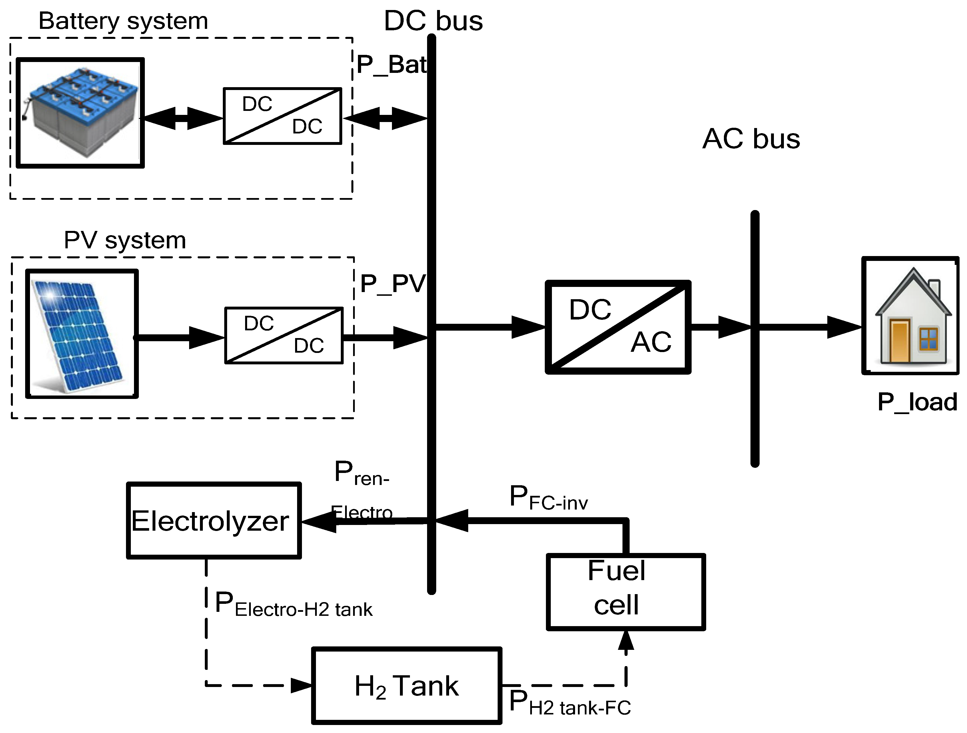
The configuration of a stand-alone microgrid is illustrated in Figure 1. This is a general configuration that contains a PV power plant with FC. Moreover, a battery was included as a storage device. This system is designed to introduce an essential solution in remote areas.
2.2. Complete Microgrid Mathematical Model
2.2.1. Solar System
The solar system is modeled considering the variations of the produced power from the PV solar system with both irradiance and temperature. The model of the produced power is illustrated using Equations (1) and (2) [10,11].
where NPV and PPV_rated indicate the PV modules number and the nominal power of each, while ηPV and ηwire represent the efficiencies of the PV and connected wire, respectively. Moreover, G(t) and Gnom represent solar irradiance at the operating temperature and the standard one of 1000 W/m2, respectively. ΒT, TC, and TC_nom indicate temperature coefficient module, cell temperature, and standard temperature of 25 °C, respectively. Furthermore, the cell temperature is estimated as follows:
where Tambient and TTest denote the module’s ambient and tested temperatures, respectively.
2.2.2. Battery Storage Unit
Battery storage units have been used to mitigate the variation of the PV and wind-generated power, which vary with many uncontrolled operation conditions, for instance, irradiance, temperature, and wind speed. The usage of storage units will be useful to control power flow to loads. Several studies reported that the lead-acid battery has a wide usage for such applications because of its availability and competitive price with respect to other battery types. Factors affecting the battery bank sizing include lifetime, temperature as well as depth of discharge (DOD) [10,24]. The capacity boundary of the battery banks can be weighed considering the state of charge (SOC).
Moreover, SOC respecting the storage banks is determined using the charging and discharging energy. The state of charge is estimated using time as per Equations (3)–(6). There are two modes of operation: the first one is the charging mode, while the other is the discharging mode. In the period of charging, the charged energy is calculated as follows:
where ECH(t) represents the charged energy during Δt, which is one hour at instant t. Pload(t) represents the load power at the same instant t, while ηconv and ηCH are the efficiencies of converter and charging, respectively. Moreover, the state of charge is estimated as
where SOC (t) and SOC(t − 1) denote battery SOCs at two instances of and t − 1, one-to-one. Additionally, σ denotes the rate of self-discharging. While the discharging mode energy and SOC can be calculated as follows:
where EDIS(t) represents the discharging energy at a time t. At the same time, ηDIS denotes the discharging efficiency of the battery.
2.2.3. Electrolyzer
The electrolyzer is implemented based on the water-electrolysis concept, producing hydrogen and oxygen by flowing a DC-current among two electrodes. Subsequently, the hydrogen is gathered on all sides of the anode surface. According to the water electrolyzer mentioned by [25,26,27], the generated hydrogen is gathered at a pressure of 30 bar. This value is very high as compared with the produced one from the reactant-pressure to supply the proton exchange membrane fuel cell (PEMFC). In many studies, the generated hydrogen from the electrolyzer can be supplied to the hydrogen tank, or its pressure is increased to 200 bar by a compressor to boost the energy stored density [25]. The other studies stated that the hydrogen evaluated from the electrolyzer is applied to a low-pressure tank until it is charged; therefore, a compressor is utilized to force the stored hydrogen to a high-pressure tank. Hence, the energy depleted by the compressor is decreased because it is not in the process of launching the whole time [25,26]. In this work, the generated hydrogen is applied to the hydrogen tank. The electrolyzer can be simulated via the transmitted power from the DC-bus to the hydrogen tank, and it can be expressed by the following formula [25,26,27],
where PElectro−tank is the output electrolyzer power that is injected into the hydrogen tank. Pren−Electro is the output electrolyzer power. The ηElectro is the electrolyzer efficiency.
2.2.4. Hydrogen Tank
In the proposed work, the hydrogen tank is simulated via the energy-stored quantity (Etank) in the hydrogen tank at a time t. The Etank can be formulated as follows [25]:
where Ptank−FC(t) is the equivalent power that pulled out from the hydrogen tank and applied to the fuel cell (FC), and ηstorage is the efficiency of the storage tank, and it indicates the losses, and it can be provided as 95% for all operating scenarios [25]. Δt is the interval of the simulation process, and it is deemed to be one hour in the proposed work.
The mass of stored hydrogen Mtank in the tank can be expressed by the following equation [25,26,27]:
where HHVH2 is the higher heating value of hydrogen (HHV). In line with [26], the amount of HHV is deemed as 39.7 kWh/m2. The energy stored in the tank comes among a predefined upper and lower limit of the tank capacity. According to some issues related to hydrogen nature, there is a recommendation that the low quantity (lower limit) of stored hydrogen is not discharged and can be considered here by 5%. Consequently,
where Mtank is ranged between the upper Mtank,max and lower Mtank,min limits of hydrogen tank at time t.
2.2.5. Fuel Cell (FC)
The electrolysis of the hydrogen FC is working in reverse to generate electric current when the hydrogen is recombined with the oxygen. However, the PEMFC is manufactured in large generating sizes to be reliable with a short-power release time of around 1–3 s [25].
In this work, the efficiency of the FC (ηFC) is considered to be 50% constant value. Therefore, the produced power can be estimated in a simple way based on the input power Ptank−FC and ηFC of the FC by the following formula:
2.2.6. DC/AC Converter
The main roles of the inverter are to convert the produced DC power from renewable sources and the FC source into AC power, besides exceeding the supplied power to the grid. In this study and based on [28], the inverter efficiency (ηinv) is supposed to be 90% as a constant value. Hence, the output power of the inverter can be estimated using the following equation:
2.3. Energy Flow Scenarios
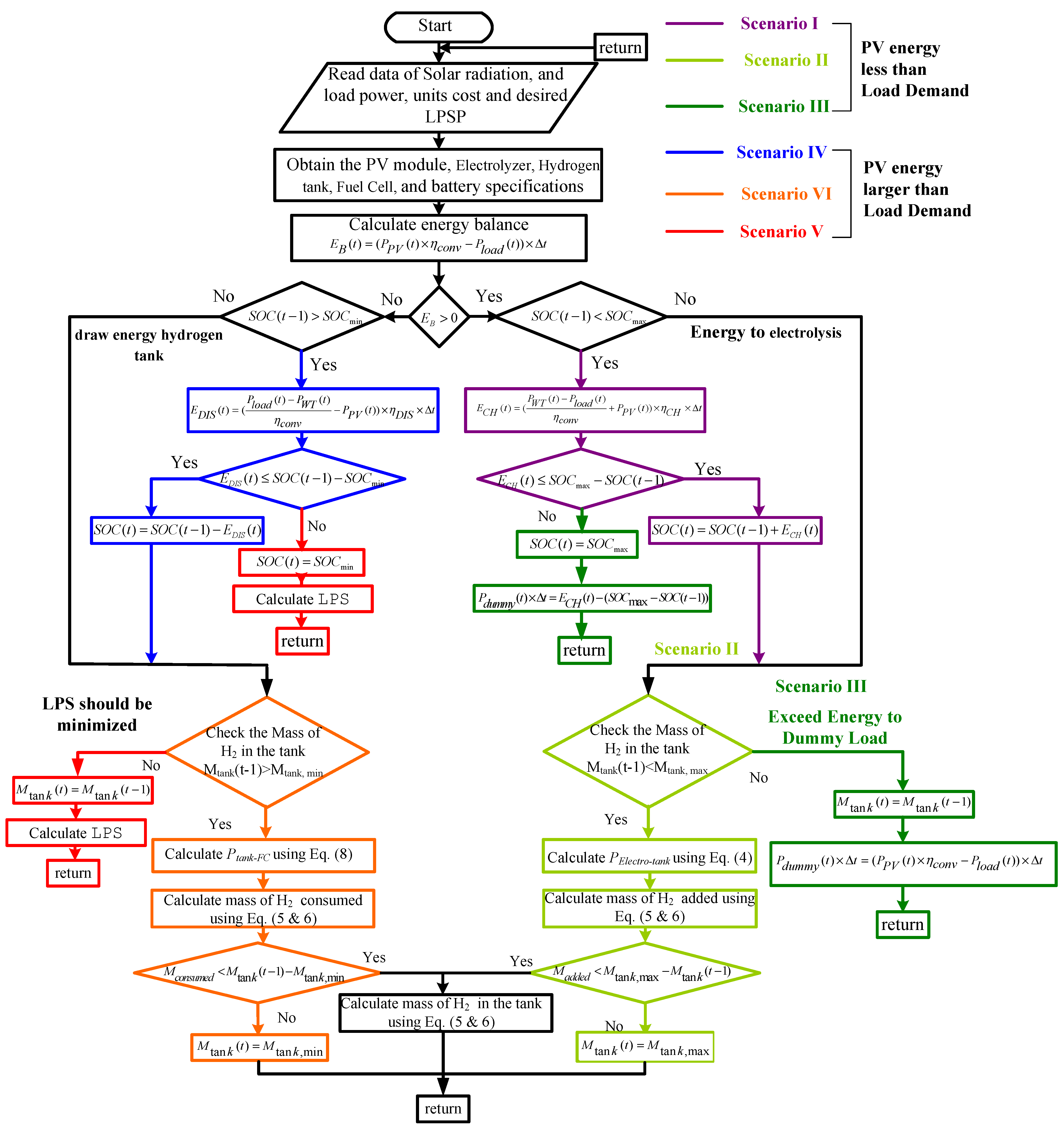
The methodology of the energy management system in a microgrid is planned to ensure continued energy covering the load demand. The energy management can be concluded in the following six scenarios. The first three scenarios are related to the generated energy from PV being less than the demand load; in this case, the battery and FC should be operated to cover the load demand energy. The other three scenarios are related to the generated energy from PV being larger than the demand load; in this case, the battery and FC should be operated to store the extra energy.
2.3.1. Case 1
- Scenario I:
The battery should operate in the discharging mode of the battery to feed the load demand when renewable energy does not cover it. So, in this case, the load power shearing is as follows:
- Scenario II:
Continuously; if the renewable energy and battery do not cover the load demand, this is the time of FC operation. The generated power from the FC is estimated as
- Scenario III:
Continuously; if the renewable energy, battery, and FC, does not suffice the load needs, there is a shortage in the energy to supply the load needs. The LPS should be calculated to be minimized. Moreover, a solution of DG may be used.
2.3.2. Case 2
- Scenario IV:
On the other hand, when the generated energy from renewables exceeds the load demand, the battery will be operated in charging mode. The power fellow in this scenario will be demonstrated as follows:
- Scenario V:
Sometimes the battery is full in the time of the renewable energy is exceeds the load demand. In this scenario, the extra energy will be stored in the FC tank. The power fellow in this interval is expressed as:
- Scenario VI:
Sometimes, the battery is full in the time of the renewable energy is exceeds the load demand. The extra energy is supplied to the dummy load in this scenario. The dummy load in this interval is expressed as
All scenarios can be visualized as the flowchart of Figure 2.
2.4. Sizing of Microgrid Problem Formalization
2.4.1. Optimized Objective Function Indices
There are many indices that should be minimized to ensure the excellent design of the microgrid. Three indices have been considered, which are (1) the cost of rnergy (COC), (2) loss of power supply probability (LPSP), and (3) the dummy load (Pdummy) [10,29,30]. Therefore, the objective function is composed of the four indices with a weighted ratio. The system will be designed in order to minimize the weighted objective function.
- (1)
- Cost of Energy (COC)
The net present cost (NPC) is utilized to estimate the whole cost of the hybrid micro-grid. The system annual cost of investment Cann_tot can be expressed by the following formula:
where, , , and are the annual costs of the system components, system components’ replacements, operation and maintenance, respectively.
- (a)
- The Annual Capital Cost of the Microgrid System
The capital recovery factor (CRF) is utilized changing the initial investment to annual capital costs based on the following equation:
where r and Msys are the rate of interest (%) and the life span of the whole hybrid system under study.
The annual capital cost of the individual subsystems is evaluated using the next expressions,
where , , , and are the initial capital cost of PV system integration, the initial cost of the battery bank, and the initial cost of all components of FC, respectively. MPV, Mbatt, and MFC are the lifetime of PV modules, battery banks, and FC, consequently.
Therefore, the annual capital investment cost of the hybrid system is formulated as follows:
where , , , and are the annual-capital-cost share of the integration of the PV, FC, battery bank, and converter, consequently.
- (b)
- The Operation and Maintenance Cost
The operation and maintenance cost of the proposed scheme is estimated in the following form:
where, , , , and are the operation and maintenance costs of PV, battery banks, converter, and FC per unit time, respectively. , , , and are the operating time of PV, battery banks, converter, and FC, respectively.
- (c)
- The Annual Replacement Cost
The replacement cost of the hybrid system components during its lifetime is determined by the next formula [10,11,12,13,14,15,16,17,18,19,20,21,22,23,24,25,26,27],
where, , , , and nrep are the inflation-rate of replacement, the unit’s size utilized in the system, the cost of the replaced units, besides the number of the replacements during the project time Msys.
Hence, the net present cost (NPC) is expressed as follows,
The cost of energy (COE) is defined as the generated electrical energy cost from the hybrid system in (USD/kWh). The COE is expressed as
- (2)
- Loss of Power Supply Probability (LPSP)
The LPSP is defined as a design factor. It takes the measurements of the insufficient operation probability of the power supply in the case of the hybrid microgrid is unsuccessful in satisfying the energy demand. The loss of power supply is given by the following formula:
LPSP is known as a practical index to estimate the reliability in the issues of the optimum capacity of hybrid renewable energy systems. Thus, the LPSP is evaluated based on the summation of the overall load demand within all study periods, and it can be mathematically written as follows:
2.4.2. The Proposed Objective Function
The objective function (OF) of this work is proposed to minimize the COE, LPSP, in addition to the dummy load (Pdummy) based on the optimization technique. Subsequently, the OF is created in the following expression:
In this work, the weighting factors Ψ1, Ψ2, and Ψ3 are selected based on trial and error to achieve the best results. This selection is considered according to the following conditions; weighting factors summation are equal to unity, their values ϵ (0, 1), and the Ψ2 value must be higher than Ψ1, and Ψ3 values for ensuring the whole system reliability. Therefore, the produced Ψ1, Ψ2, and Ψ3 values are 0.2, 0.6, and 0.2, respectively.
2.4.3. Design of Constrains for Optimization
In off-grid hybrid systems, the operation of the system components must be considered based on constraints. To ensure the optimal operation of the system to confirm the condition in Equation (29), the generated energy at a time (t) is balanced with the energy consumed by the load. This constraint can be expressed as follows:
Equation (30) is considered as one of the optimization policies to assure that the power storage per hour by hydrogen tank at a time should be performed within limits, and it can be represented as
Avoiding the over/under charging issues, the SOS of the battery bank is constrained between its maximum and minimum values. Where the is considered the full size of the battery, on the other hand, the is subjected to the depth of discharge. This condition can be illustrated by Equations (31) and (32):
The LPSP can be lower than the system indicator of predefined reliability (). In this work, the is equal to 0.04 [10]. This can be formulated as follows:
2.5. Optimization Algorithms
2.5.1. Bat Optimization (BAT)
Bat algorithm (BA) is inspired by the echolocation manner of bats detecting their foods [31]. Only mammals can detect their prey based on sonar waves “echolocation” avoiding barriers in the darkness. Based on the echolocation attitude, bats can determine the distance of object “prey” as follows [31]:
- Based on the echolocation characteristics, the bat can detect their prey and recognize the variation between food and surrounding barriers.
- The flying bat is in a random form toward a place (xi) via velocity (vi) and frequency (Fmin), wide wavelength (λ), and loudness (Lo) for detecting the prey. It has the capability to control its pulses λ/Fmin based on pulse rate emission r via a range of 0–1 to approximate its goal.
- Based on [31], the loudness has been supposed to be ranged from maximum value (Lo) to a minimum value (Lmin).
The virtual movements of ith bat can be evaluated based on xi and vi in D-dimension. Additionally, the values of xi and vi are upgrading at each iteration, and the process can be defined as follows:
where β ϵ [0, 1] is a random vector that is extracted from a uniform distribution, and x* is the current global best solution from all bats. Locally, if a current best solution is so far, then it is generated new solutions based on a local walk randomly as formulated below:
where ε ϵ [−1, 1] is a random number, and Lt is the average of loudness at t time. In the case of the bat being very close to prey, it reduces its loudness increasing the emitted rate of pulses. It can be assumed that when a bat detected its prey, then the Lo = 1 and Lmin = 0, and it can be formulated as
where α and γ are constant values that are α > 0 and γ < 1. In addition,
Note that the initial values of Lo and ri can range between 0 and 1.
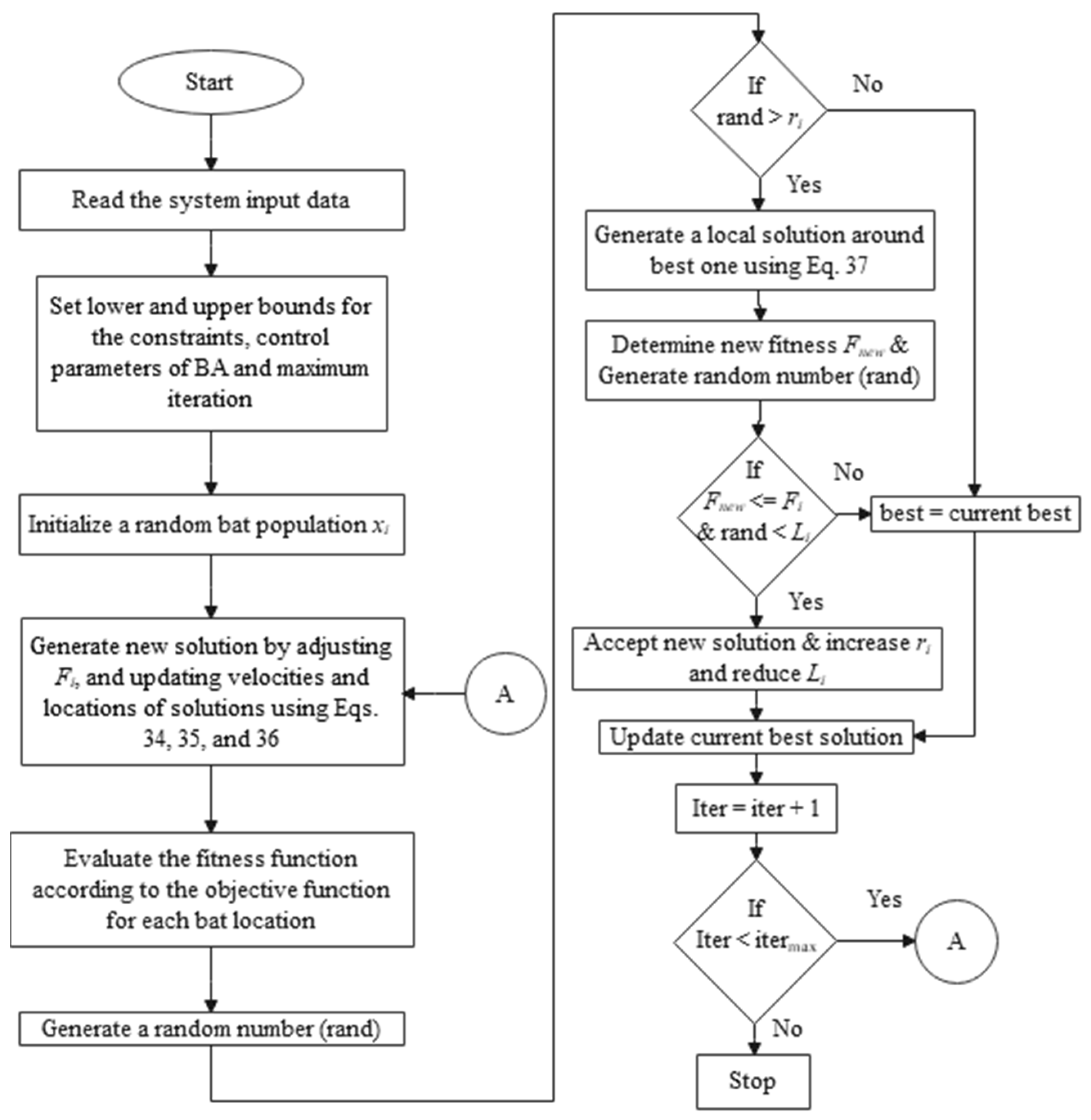
The steps of the BAT technique process can be deduced in the flowchart in Figure 3.
2.5.2. Black-Hole-Based Optimization Technique (BHB)
The BHB technique was inspired by the black-hole phenomenon [32]. It is a population-based algorithm, where a “black-hole” is known as the best solution/candidate of the population at every iteration, and the other solutions are known as “normal stars”. The basic election of the black hole is one of the genuine candidates of the population. The black hole attracts all solutions based on their current placement, including a random number. The normal stars can be pulled around the black hole after the initializing process. In addition, the black hole will allow the too-closed stars to be gone forever.
The proposed BHB can be formulated in the following process [32]:
Process 1: Initializing. For stars, a population size “N” has been generated with random sittings in a research space that is distributed in limited upper and lower boundaries.
Process 2: Run the program performing all constraints for every star of the population. If the satisfied star constraints, then it is workable; otherwise, it is not workable.
Process 3: Evaluate the fitness function for every workable star.
Process 4: Record the best fitness/star as the black-hole XBH star.
Process 5: Start with count t = 1.
Process 6: Alter the sitting of every star based on the following Equation (40):
where t is the iteration number, Xi is the sitting of the star at iteration t, and XBH is the sitting of the black-hole in the search space.
Process 7: If a star gets a sitting where the parameters of the proposed design are lower than previous, then update their sittings as the following:
Process 8: Calculate the radius of events horizon R based on the following Equation (42):
where the F(XBH) is the fitness content of the black hole, and the F(Xi) is the fitness content of ith star.
Process 9: If a star passes the event horizon R of the black hole, alter it with a new one in a random sitting in the space. Otherwise, go to process 6.
Process 10: Raise generation count t = t + 1.
Process 11: If t ≤ tmax, start again from process 6. Otherwise, stop.
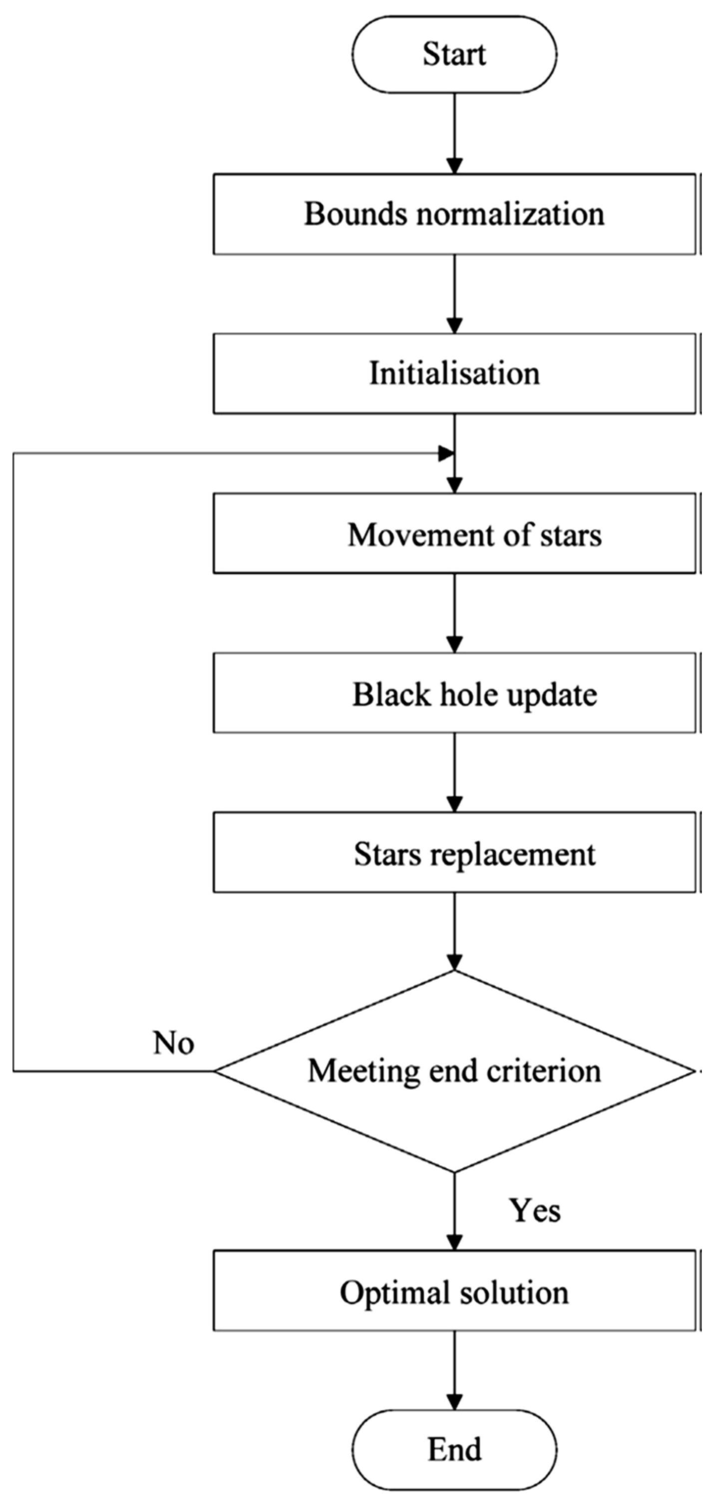
According to the above process, the flowchart of the proposed BHB technique is shown in Figure 4.
2.5.3. Equilibrium Optimizer (EQ)
The EQ technique was created by Farmarzi in 2020 [33]. It is a meta-heuristic technique that simulates the dynamics and equilibrium mass balance schemes. This technique can be initiated with concentrations of ith particles “C” via special number and dimensions as recorded in the following equation:
where the Bl and Bu are the lower and upper boundaries of the search space, the r ϵ (0, 1) is uniform random.
Based on evaluating the fitness function, the “C” can be upgraded via computing the equilibrium solutions to deduce the best candidates. The upgrading process of the EQ technique can be deduced in the following form:
where the exponential term “E” and the rate of generation “G” can be known as
where a1 and a2 are constants and equals 2 and 1, respectively, m1 ϵ (0, 1) is random vector, iter and max_iter are the iteration number and the maximum one respectively. r1 and r2 ϵ [0, 1] are random numbers, GP = 0.5 and it is the generated probability.
Within every upgrading, the proposed fitness function is calculated for every particles’ concentration to evaluate their states and to include the best so far particles. Based on Equation (44), the upgrading process of every concentration particle re-generated depends on the sharing of three sections. The first section is random, and it is extracted from the equilibrium pool. The other sections focus on the variations in concentrations. The last two sections are in charge of the exploitation accuracy and the global searching in the research space to deduce the optimum issues, respectively.
Figure 5 illustrates the flowchart of the proposed EQ technique.
2.6. Case Study
To evaluate the energy management system based on various optimization algorithms, a real study case was introduced with the purpose of designing a hybrid renewable energy system, and it was selected in the Dobaa region in Egypt. The microgrid has been designed for the emergency operation of the projected nuclear station of Dobaa in Egypt at Geographical coordinates of 30.040566, 26.806641 (30°02′26″, 26°48′24″) [34]. For the emergency operation, the microgrid should be disconnected from the electrical grid. The location of the site, as mentioned, is in the Dobaa nuclear station, as shown in Figure 6. The data of horizontal solar radiation are presented in Figure 7. As the temperature represents an essential factor for the PV performance, the monthly average temperature is shown in Figure 8. The estimated emergency average load demand per month and the estimated load curve per day are introduced in Figure 9 and Figure 10. The load curve was calculated and estimated based on the expected load of the plant in an emergency. It should be noted the residential loads in the period from 7 pm to 10 pm. Other domestic facilities were recorded. The average load and the maximum load demand were 265 kW and 420 kW, respectively.
3. Results and Discussions
MATLAB package was used in order to determine the optimal configuration-based individual optimization algorithms. For each algorithm, the maximum iterations and search agents number were considered to be 200 and 30, respectively. According to this work, the capacity of the proposed microgrid (hybrid system) is realized as PV rated power and their modules number, the mass of hydrogen tank, number of battery units, the rated power of the electrolyzer and fuel cell. The optimization algorithm should determine the configuration of the energy system to minimize the objective function. The data specifications of the system components can be found in [11] and are given in Table 1.
3.1. The Optimal Configuration of Energy System
Table 2 displays the comprehensive outcomes of the optimization procedures of BAT algorithm, equilibrium optimizer, and black hole algorithm. The minimum value of each is highlighted in the table for visualizing the best results. The minimum best objective function was obtained by the EQ algorithm. Moreover, the best COE is 0.289129, which is obtained by BAT algorithm, while LPSP and dummy Load indices with BAT algorithm are 0.045548 and 0.113331, respectively, which indicate more load is not covered in certain periods and other periods; the dummy load index shows that more surprise energy is dissipated. The results of the EQ algorithm for LPSP and dummy load are 0.043986 and 0.113607, respectively. This indicates that although the COE is higher than that of the BAT algorithm, the LPSP of 0.0436418 was obtained, which results from more uninterrupted energy to the load.
The net present values are 546067.9, 550426, and 571437.7 for BAT, EQ, and BHB optimizers, respectively. Although the net present value of EQ is higher than that of BAT by 0.9664%, the recommended design is that of the EQ algorithm. This recommendation is because of the decrease of the LPSP with the EQ algorithm rather than that of the BAT algorithm. In general, the two designs based on BAT and EQ algorithms can be considered concerning the priority of LPSP or COE. Figure 11 and Figure 12 visualize the obtained results of the various configurations of the microgrid based on the three algorithms.
3.2. Performance of Different Algorithms
Figure 13 illustrates the convergence curves for the proposed BAT, EQ, and BHB techniques. From this figure, the proposed optimizers can achieve the optimal values of the recommended objective function to be 0.112231, 0.1074, and 0.108078 for BAT, EQ, and BHB algorithms, respectively, which indicated that the EQ has the best minimum objective function. Nevertheless, Figure 13 demonstrates that the EQ is the fastest one compared with BAT and BHB optimization techniques. The detailed results of the three algorithms are presented in Section 3.3.
3.3. Statistical Results
The BAT algorithm was implemented for 30 individual runs. The statistical results of the BAT, EQ, and BHB algorithms are listed in Table 3. The results show that the minimum and maximum obtained cost functions of the BAT algorithm are 0.112231 and 0.13043, respectively, while the stranded division and the average obtained results of the BAT algorithm are 0.117865 and 0.469301, respectively. On the other hand, the statistical results show that the obtained minimum and maximum values of the cost functions of the EQ algorithm are 0.1074 and 0.112216, respectively, while the stranded division and the average values EQ algorithm are 0.223387 and 0.110812, respectively. Moreover, the table shows that the minimum and maximum obtained cost functions of BHB are 0.108078 and 0.124731, respectively. In comparison, the stranded division and the average results of BHB are 0.41938 and 0.114019, respectively. The obtained results show that the best-obtained results are acceptable for all algorithms, but EQ and BHB algorithms are better algorithms rather than BAT. Furthermore, the statistical indices show that the divisions between the results of individual runs of the BAT algorithm are bigger than those of the EQ and BHB.
The convergence curves of the 30 individual runs are shown in Figure 14 for the three algorithms. Furthermore, the boxplot of the best objective functions is shown in Figure 13. On the other side, the Wilcoxon signed-rank test was performed to validate the application of the BAT, EQ, and BHB algorithms. The results show that the value of the rank h is 1 for the three algorithms, which indicates that the test rejects the null hypothesis of zero median. Moreover, the p is 1.73 × 10⁻⁶, 1.82 × 10⁻⁵, and 1.73 × 10⁻⁶, which proves the robustness of the BAT, EQ, and BHB algorithms, respectively. The box plot has been plotted for the three algorithms for more visualization of the performance of the three algorithms, as shown in Figure 15. The figure demonstrates the superiority of the EQ algorithm for optimizing the size of the microgrid for the considered case study.
3.4. Operation of the Microgrid
The operation of the microgrid is investigated in this part. The performance of the microgrid is shown in Figure 16. Figure 16 illustrates the generated power change per hour of proposed hybrid system components at the optimal case of the EQ technique. Figure 16a shows the load demand (Pload), the hole generated power from the renewable energy (PPV), and the difference between the renewable generation and the load (Pdiff). Moreover, Figure 16b illustrates the battery charge, discharge, tank, and fuel cell during the operation period.
Furthermore, Figure 16c displays the dummy load and LPSP. Because of the design conditions, it is not easy to realize the optimization requirements even though keeping LPSP or dummy load to be zero. Through the hourly period of the high generated power from renewables, the extra energy is utilized to charge the battery and fill the hydrogen tank. For more clearance of the energy management concept behindhand the optimization techniques, the simulated numeric results are focused on the hybrid system performance for one day at the optimal conditions of their operation.
Figure 17 displays the results for a certain day regarding the optimum capacity from the EQ optimizer. According to Figure 17a, it is noticeable that the per diem curve of load demand includes two topmost points. The first one is nearby at 1 pm, where the temperature is high during this time. Hence, all existing equipment is required to be in service to decrease the air temperature. The second topmost point is nearby at 6 pm after the sunset. Within the nighttime till the early hours, the generated power from the renewable sources is very low; consequently, the battery and full cell are operating to cover the electricity demand. If the same conditions are still, the LPSP, as shown in Figure 17c, has a value. During the sunrise, around 6 am, the generated power from the PV station increases. Consequently, the electric energy over the load needs is utilized to charge the battery and fill up the hydrogen tank. Through the daytime between 2 pm and 6 pm, the generated power from the nontraditional sources is higher than the load needs. Therefore, the excess power is used to fill the tank and charge the battery, as shown in Figure 17b. The hydrogen increased until the tank amounted to its maximum limit and the battery charging. When the battery and the tank also are fully charged, the excess power is pushed into the dummy load, as shown by Figure 17c.
4. Conclusions and Future Directions
In this paper, a stand-alone microgrid has been designed to feed emergency loads of a nuclear power plant using recent optimization algorithms of equilibrium optimizer (EQO), bat optimization (BAT), and black hole (BH). A comprehensive comparison between the ability and performance of the algorithms was conducted to solve the problem of microgrids design. A configuration of a microgrid consisting of a PV plant with FC and battery storage systems was optimally designed, and the possibility of integrating with a nuclear power plant to enhance the emergency power supplies was studied. The optimization algorithms are individually used to optimize and size the energy systems to minimize the cost and ensure the optimized microgrid’s reliability. The energy systems were modeled and evaluated in MATLAB.
The results show that the EQ algorithm has a better performance than the other algorithms considering the best objective function value. The objective function was improved to 0.1074 using the EQ algorithm, while its values were 0.112231 and 0.108078 with BAT and BHB. However, the COE of the EQ-based results is higher than the BAT algorithm, while it is lower than the BHB. On the other hand, the reliability index of the EQ algorithm is better than the BAT algorithm, which is the main reason to increase the COE of the EQ algorithm. The results of BHB indicate that the LPSP is a smaller one with respect to the EQ and BAT, while the dummy load of the BHB is higher than those of the BAT and EQ algorithms. Finally, the designed microgrid based on the EQ and BHB is recommended based on the obtained results of the simulation of the microgrid operation and statistical analyses. It should be remarked that the storage energy cost is considered one of the main reasons to increase the COE and affect the system reliability. Using other renewable energy sources such as bioenergy or wind energy may enhance the system performance. Therefore, in future work, different configurations of off-grid and grid-connected microgrids should be designed to include a wind power plant, bioenergy, and/or diesel generator to increase the system’s reliability and reduce the COE.
Author Contributions
Conceptualization, A.A.Z.D. and M.M.Z.; Methodology, A.A.Z.D. and M.A.T.; Software, A.A.Z.D.; Data curation, A.A.Z.D., A.M.E.-R. and M.A.T.; Formal analysis, A.A.Z.D., A.M.E.-R. and M.A.T.; Visualization, A.A.Z.D., A.M.E.-R. and M.A.T.; Investigation, A.M.E.-R. and M.M.Z.; Analysis, A.A.Z.D. and A.M.E.-R.; Writing—original draft, A.A.Z.D. and M.A.T.; Writing—review and editing, A.A.Z.D., A.M.E.-R. and M.M.Z. All authors have read and agreed to the published version of the manuscript.
Funding
This research received no external funding.
Institutional Review Board Statement
Not applicable.
Informed Consent Statement
Not applicable.
Data Availability Statement
Not applicable.
Acknowledgments
The researchers (Ahmed A. Zaki Diab and Mohamed A. Tolba) are funded by a full scholarship (Mission 2020/21 and Mission 2019/20) from the Ministry of Higher Education of Egypt. However, the current research work is not funded by the mentioned Ministry in Egypt or any other organization/foundation.
Conflicts of Interest
The authors declare no conflict of interest. Non-financial competing interest.
References
- The Arab Republic of Egypt, Ministry of Electricity and Energy. Egyptian Electricity Holding Company_Annual Report 2015–2016. Available online: http://www.moee.gov.eg/english_new/report.aspx (accessed on 10 April 2021).
- Sultan, M.H.; Kuznetsov, O.N.; Diab, A.A.Z. Site selection of large-scale grid-connected solar PV system in Egypt. In 2018 IEEE Conference of Russian Young Researchers in Electrical and Electronic Engineering (EIConRus); IEEE: New York, NY, USA, 2018; pp. 813–818. [Google Scholar]
- Sultan, H.M.; Diab, A.A.Z.; Oleg, N.K.; Irina, S.Z. Design and evaluation of PV-wind hybrid system with hydroelectric pumped storage on the National Power System of Egypt. Glob. Energy Interconnect. 2018, 1, 301–311. [Google Scholar]
- The Official Website of the Ministry of Electricity and Energy. Available online: http://www.moee.gov.eg (accessed on 10 April 2021).
- Tolba, M.A.; Diab, A.A.Z.; Tulsky, V.N.; Abdelaziz, A.Y. LVCI approach for optimal allocation of distributed generations and capacitor banks in distribution grids based on moth–flame optimization algorithm. Electr. Eng. 2018, 100, 2059–2084. [Google Scholar] [CrossRef]
- Diab, A.A.Z.; Sultan, H.M.; Kuznetsov, O.N. Optimal sizing of hybrid solar/wind/hydroelectric pumped storage energy system in Egypt based on different meta-heuristic techniques. Environ. Sci. Pollut. Res. 2019, 27, 32318–32340. [Google Scholar] [CrossRef] [PubMed]
- Shouman, R.; El Shenawy, E.T.; Khattab, N.M. Market financial analysis and cost performance for photovoltaic technology through international and national perspective with case study for Egypt. Renew. Sustain. Energy Rev. 2016, 57, 540–549. [Google Scholar] [CrossRef]
- Kamel, O.M.; Abdelaziz, A.Y.; Zaki Diab, A.A. Damping Oscillation Techniques for Wind Farm DFIG Integrated into Inter-Connected Power System. Electr. Power Compon. Syst. 2020, 48, 1551–1570. [Google Scholar] [CrossRef]
- Ngan, M.S.; Tan, C.W. Assessment of economic viability for PV/wind/diesel hybrid energy system in Southern Peninsular Malaysia. Renew. Sustain. Energy Rev. 2012, 16, 634–647. [Google Scholar] [CrossRef]
- Diab, A.A.Z.; Sultan, H.M.; Mohamed, I.S.; Kuznetsov, O.N.; Do, T.D. Application of different optimization algorithms for optimal sizing of PV/wind/diesel/battery storage stand-alone hybrid microgrid. IEEE Access 2019, 7, 119223–119245. [Google Scholar] [CrossRef]
- Diab, A.A.Z.; El-ajmi, S.I.; Sultan, H.M.; Hassan, Y.B. Modified farmland fertility optimization algorithm for optimal design of a grid-connected hybrid renewable energy system with fuel cell storage: Case study of Ataka, Egypt. Int. J. Adv. Comput. Sci. Appl. 2019, 10, 119–132. [Google Scholar] [CrossRef]
- Rezk, H.; Al-Dhaifallah, M.; Hassan, Y.B.; Ziedan, H.A. Optimization and Energy Management of Hybrid Photovoltaic-Diesel-Battery System to Pump and Desalinate Water at Isolated Regions. IEEE Access 2020, 8, 102512–102529. [Google Scholar] [CrossRef]
- Tran, Q.T.; Davies, K.; Sepasi, S. Isolation Microgrid Design for Remote Areas with the Integration of Renewable Energy: A Case Study of Con Dao Island in Vietnam. Clean Technol. 2021, 3, 804–820. [Google Scholar] [CrossRef]
- Xiang, Y.; Han, W.; Zhang, J.; Liu, J.; Liu, Y. Optimal sizing of energy storage system in active distribution networks using Fourier–Legendre series based state of energy function. IEEE Trans. Power Syst. 2017, 33, 2313–2315. [Google Scholar] [CrossRef]
- Lu, X.; Wang, H. Optimal sizing and energy management for cost-effective PEV hybrid energy storage systems. IEEE Trans. Ind. Inform. 2019, 16, 3407–3416. [Google Scholar] [CrossRef]
- Gonzalez, A.; Riba, J.R.; Rius, A.; Puig, R. Optimal sizing of a hybrid grid-connected photovoltaic and wind power system. Appl. Energy 2015, 154, 752–762. [Google Scholar] [CrossRef] [Green Version]
- Biswas, A.; Kumar, A. Techno-Economic Optimization of a Stand-alone PV/PHS/Battery systems for very low load situation. Int. J. Renew. Energy Res. 2017, 7, 844–856. [Google Scholar]
- Kaab, A.; Sharifi, M.; Mobli, H.; Nabavi-Pelesaraei, A.; Chau, K.W. Use of optimization techniques for energy use efficiency and environmental life cycle assessment modification in sugarcane production. Energy 2019, 181, 1298–1320. [Google Scholar] [CrossRef]
- Acevedo-Arenas, C.Y.; Correcher, A.; Sánchez-Díaz, C.; Ariza, E.; Alfonso-Solar, D.; Vargas-Salgado, C.; Petit-Suárez, J.F. MPC for optimal dispatch of an AC-linked hybrid PV/wind/biomass/H2 system incorporating demand response. Energy Convers. Manag. 2019, 186, 241–257. [Google Scholar] [CrossRef]
- Ciardiello, A.; Rosso, F.; Dell’Olmo, J.; Ciancio, V.; Ferrero, M.; Salata, F. Multi-objective approach to the optimization of shape and envelope in building energy design. Appl. Energy 2020, 280, 115984. [Google Scholar] [CrossRef]
- Gassar, A.A.; Koo, C.; Kim, T.W.; Cha, S.H. Performance Optimization Studies on Heating, Cooling and Lighting Energy Systems of Buildings during the Design Stage: A Review. Sustainability 2021, 13, 9815. [Google Scholar] [CrossRef]
- Chang, X.; Xu, Y.; Gu, W.; Sun, H.; Chow, M.-Y.; Yi, Z. Accelerated Distributed Hybrid Stochastic/Robust Energy Management of Smart Grids. IEEE Trans. Ind. Inform. 2021, 17, 5335–5347. [Google Scholar] [CrossRef]
- Chang, X.; Xu, Y.; Sun, H.; Khan, I. A distributed robust optimization approach for the economic dispatch of flexible resources. Int. J. Electr. Power Energy Syst. 2021, 124, 106360. [Google Scholar] [CrossRef]
- Ekren, O.; Ekren, B.Y. Size optimization of a PV/wind hybrid energy conversion system with battery storage using simulated annealing. Appl. Energy 2010, 87, 592–598. [Google Scholar] [CrossRef]
- Garcia, R.S.; Weisser, D. A wind–diesel system with hydrogen storage: Joint optimization of design and dispatch. Renew. Energy 2006, 31, 2296–2320. [Google Scholar] [CrossRef]
- El-Sharkh, M.Y.; Tanrioven, M.; Rahman, A.; Alam, M.S. Cost related sensitivity analysis for optimal operation of a grid-parallel PEM fuel cell power plant. J. Power Sources 2006, 161, 1198–1207. [Google Scholar] [CrossRef]
- Kashefi, K.; Riahy, G.H.; Kouhsari, S.M. Optimal design of a reliable hydrogen-based stand-alone wind/PV generating system, considering component outages. Renew. Energy 2009, 34, 2380–2390. [Google Scholar] [CrossRef]
- Khan, M.J.; Iqbal, M.T. Pre-feasibility study of stand-alone hybrid energy systems for applications in Newfoundland. Renew. Energy 2005, 30, 835–854. [Google Scholar] [CrossRef]
- Mohamed, M.; Eltamaly, A.; Alolah, A.; Hatata, Y.A. A novel framework-based cuckoo search algorithm for sizing and optimization of grid-independent hybrid renewable energy systems. Int. J. Green Energy 2018, 16, 86–100. [Google Scholar] [CrossRef]
- Ramli, M.A.M.; Bouchekara, H.R.E.H.; Alghamdi, A.S. Optimal sizing of PV/wind/diesel hybrid microgrid system using multiobjective self-adaptive differential evolution algorithm. Renew. Energy 2018, 121, 400–411. [Google Scholar] [CrossRef]
- Yang, X.-S. A new meta heuristic bat-Inspired algorithm. In Nature Inspired Cooperative Strategies for Optimization (NISCO 2010); Gonzalez, J.R., Ed.; Studies in Computational Intelligence; Springer: Berlin/Heidelberg, Germany, 2010; pp. 65–74. [Google Scholar]
- Bouchekara, H.R.E.H. Optimal design of electromagnetic devices using a black-Hole-Based optimization technique. IEEE Trans. Magn. 2013, 49, 5709–5714. [Google Scholar] [CrossRef]
- Faramarzi, A.; Heidarinejad, M.; Stephens, B.; Mirjalili, S. Equilibrium optimizer: A novel optimization algorithm. Knowl.-Based Syst. 2020, 191, 2020. [Google Scholar] [CrossRef]
- Available online: Solargis.com (accessed on 15 April 2021).
Figure 1.
Arrangement of the studied microgrid.

Figure 2.
Scenarios of energy management flowchart.

Figure 3.
Flowchart of BAT technique.

Figure 4.
Flowchart of BHB technique.

Figure 5.
Flowchart of EQ Technique.

Figure 6.
Location of the studied microgrid.

Figure 7.
Solar radiation for the study area.

Figure 8.
Temperature for the study area.

Figure 9.
The average load demand per month.

Figure 10.
The load curve per day of the study area.

Figure 11.
Indices of the energy system based on various algorithms.

Figure 12.
Configuration of the energy system based on various algorithms.

Figure 13.
Convergence curves of the three algorithms.

Figure 14.
Convergence curves of the three algorithms over 30 runs: (a) 30-run convergence curves of BAT, (b) 30-run convergence curves of EQ, and (c) 30-run convergence curves of BHB.
Figure 14.
Convergence curves of the three algorithms over 30 runs: (a) 30-run convergence curves of BAT, (b) 30-run convergence curves of EQ, and (c) 30-run convergence curves of BHB.

Figure 15.
Box plots of the three algorithms over 30 runs: (a) box plot of BAT, (b) box plot of EQ, and (c) box plot of BHB.
Figure 15.
Box plots of the three algorithms over 30 runs: (a) box plot of BAT, (b) box plot of EQ, and (c) box plot of BHB.

Figure 16.
The results for the operation of the microgrid over one year considering the optimal configuration based on EQ technique. (a) Load, PV, and the different power. (b) Performance of the charging and discharging of the storage units for the battery and FC. (c) Dummy load and LPSP.
Figure 16.
The results for the operation of the microgrid over one year considering the optimal configuration based on EQ technique. (a) Load, PV, and the different power. (b) Performance of the charging and discharging of the storage units for the battery and FC. (c) Dummy load and LPSP.

Figure 17.
Numeric results of the microgrid operation for one working day via optimal configuration using EQ technique. (a) Load, PV, and the different power. (b) Performance of the charging and discharging of the storage units for the battery and FC. (c) Dummy load and LPSP.
Figure 17.
Numeric results of the microgrid operation for one working day via optimal configuration using EQ technique. (a) Load, PV, and the different power. (b) Performance of the charging and discharging of the storage units for the battery and FC. (c) Dummy load and LPSP.


Table 1.
The system components’ descriptions [11].
Table 1.
The system components’ descriptions [11].
| Component | Capital Cost (USD/Unit) | Replacement Cost (USD/Unit) | O&M (USD/Unit–yr) | Lifetime (yr) | Efficiency (%) | Unit |
|---|---|---|---|---|---|---|
| PV array | 7000 | 6000 | 20 | 20 | 0.15 | 1 kW |
| Electrolyzer | 2000 | 1500 | 25 | 20 | 75 | 1 kW |
| Hydrogen tank | 1300 | 1200 | 15 | 20 | 95 | 1 kg |
| Fuel cell | 3000 | 2500 | 175 | 5 | 50 | 1 kW |
| Battery bank | 146.5 | 102.55 | - | 10 | 86 | 12 V (50 Ah) |
| DC/AC converter | 800 | 750 | 8 | 15 | 90 | 1 kW |
Table 2.
Optimization parameters of microgrid configurations based on the three algorithms.
| Items | BAT | EQ | BHB | |
|---|---|---|---|---|
| Best objective function | 0.112231 | 0.1074 | 0.108078 | |
| Best solution | PV (kw) | 339.6977 | 339.6308 | 348.8188 |
| Battery | 4695.026 | 4909.019 | 4893.064 | |
| Electrolyzer (kw) | 459.6776 | 452.9702 | 491.7788 | |
| Tank (kg) | 88.80917 | 87.25968 | 107.2796 | |
| FC (kw) | 34.73013 | 34.10566 | 35.4967 | |
| COE | 0.289129 | 0.291437 | 0.302562 | |
| NPV | 546067.9 | 550426 | 571437.7 | |
| LPSP | 0.045548 | 0.043986 | 0.039623 | |
| Dummy load | 0.113331 | 0.113607 | 0.118959 | |
Table 3.
Statistical results of the three algorithms of BAT, EQ, and BHB.
| Items | BAT | EQ (Best Results) | BHB |
|---|---|---|---|
| cost_min | 0.112231 | 0.1074 | 0.108078 |
| cost_maxworst | 0.13043 | 0.112216 | 0.124731 |
| cost_mean | 0.117865 | 0.110812 | 0.114019 |
| cost_median | 0.117716 | 0.112215 | 0.113443 |
| cost_sD | 0.469301 | 0.223387 | 0.41938 |
| RE | 1.506026 | 0.762435 | 1.649028 |
| MAE | 0.005634 | 0.003412 | 0.005941 |
| RMSE | 0.007282 | 0.004053 | 0.007231 |
| eff | 95.36117 | 96.95946 | 94.91016 |
| p | 1.73 × 10⁻⁶ | 1.82 × 10⁻⁵ | 1.73 × 10⁻⁶ |
| h | 1 | 1 | 1 |
Publisher’s Note: MDPI stays neutral with regard to jurisdictional claims in published maps and institutional affiliations. |
© 2022 by the authors. Licensee MDPI, Basel, Switzerland. This article is an open access article distributed under the terms and conditions of the Creative Commons Attribution (CC BY) license (https://creativecommons.org/licenses/by/4.0/).
Share and Cite
MDPI and ACS Style
Diab, A.A.Z.; El-Rifaie, A.M.; Zaky, M.M.; Tolba, M.A. Optimal Sizing of Stand-Alone Microgrids Based on Recent Metaheuristic Algorithms. Mathematics 2022, 10, 140. https://0-doi-org.brum.beds.ac.uk/10.3390/math10010140
AMA Style
Diab AAZ, El-Rifaie AM, Zaky MM, Tolba MA. Optimal Sizing of Stand-Alone Microgrids Based on Recent Metaheuristic Algorithms. Mathematics. 2022; 10(1):140. https://0-doi-org.brum.beds.ac.uk/10.3390/math10010140
Chicago/Turabian StyleDiab, Ahmed A. Zaki, Ali M. El-Rifaie, Magdy M. Zaky, and Mohamed A. Tolba. 2022. "Optimal Sizing of Stand-Alone Microgrids Based on Recent Metaheuristic Algorithms" Mathematics 10, no. 1: 140. https://0-doi-org.brum.beds.ac.uk/10.3390/math10010140
Note that from the first issue of 2016, this journal uses article numbers instead of page numbers. See further details here.