
Well-Balanced High-Order Discontinuous Galerkin Methods for Systems of Balance Laws


1
Departamento de Análisis Matemático, Estadística e Investigación Operativa y Matemática Aplicada, Facultad de Ciencias, Universidad de Málaga, 29080 Malaga, Spain
2
Departamento de Matemáticas, Campus de Rabanales, Universidad de Córdoba, 14071 Cordoba, Spain
*
Author to whom correspondence should be addressed.
Mathematics 2022, 10(1), 15; https://0-doi-org.brum.beds.ac.uk/10.3390/math10010015
Submission received: 29 November 2021
/
Revised: 15 December 2021
/
Accepted: 16 December 2021
/
Published: 21 December 2021
(This article belongs to the Special Issue Modeling and Numerical Analysis of Energy and Environment 2021)
Abstract
:This work introduces a general strategy to develop well-balanced high-order Discontinuous Galerkin (DG) numerical schemes for systems of balance laws. The essence of our approach is a local projection step that guarantees the exactly well-balanced character of the resulting numerical method for smooth stationary solutions. The strategy can be adapted to some well-known different time marching DG discretisations. Particularly, in this article, Runge–Kutta DG and ADER DG methods are studied. Additionally, a limiting procedure based on a modified WENO approach is described to deal with the spurious oscillations generated in the presence of non-smooth solutions, keeping the well-balanced properties of the scheme intact. The resulting numerical method is then exactly well-balanced and high-order in space and time for smooth solutions. Finally, some numerical results are depicted using different systems of balance laws to show the performance of the introduced numerical strategy.
1. Introduction
We consider one-dimensional systems of balance laws of the form
Here, is the state vector taking values in the space of admissibly states ; is the flux; is a function that takes into account the geometrical source terms that are multiplied by the known function ; and contains algebraic source terms. We suppose that the system is hyperbolic, and therefore the jacobian matrix of the flux has M distinct real eigenvalues.
The system (1) often admits steady-state solutions that, in most cases, are non-trivial. Moreover, these solutions usually convey significant physical meaning. A paradigmatic example of this is the lake-at-rest solution of the well-known shallow-water equations. The correct preservation of these solutions plays an essential role in any simulation. Well-balanced (or exactly well-balanced) numerical schemes aim to preserve all or at least a relevant set of specific steady-state solutions up to machine precision. A precise definition of well-balanced method is given in Section 2.
An essential advantage of well-balanced schemes is that they can accurately resolve small perturbations to steady-state solutions with relatively coarse meshes. Indeed, if a numerical method cannot preserve stationary solutions or recover a stationary solution after a perturbation, the oscillations introduced may destroy the numerical solution for long integration times. Additionally, the numerical solution may be lost entirely if the perturbation is in the same order as the discretisation errors introduced by a non well-balanced method. Then, a finer mesh or a higher-order numerical method may be considered. Still, in this case, the computational effort can quickly become excessive. The ability of the numerical scheme to correctly preserve stationary solutions becomes then a matter of paramount importance.
The first effort to preserve stationary solution was originally introduced by Bermúdez and Vázquez-Cendón in [1] for the sallow water system, where the C-property was defined as the ability of a numerical scheme to solve a set of stationary solutions exactly or, at least, with enhanced accuracy. Since then, multiple works have been published on well-balanced numerical methods [2,3,4,5,6,7,8,9,10,11,12,13,14,15,16,17,18,19,20,21,22,23,24,25,26,27,28,29,30,31,32,33,34]. It is of interest to highlight the recent work in [35], where the authors develop high order exactly well-balanced methods for systems of conservation laws for finite volume method with both continuous and discontinuous source terms. A similar strategy is presented in [36] for finite-difference methods. This paper extends the numerical strategy introduced within the framework of finite volume methods in [35] to Discontinuous Galerkin (DG) methods, describing a general approach to preserve stationary solutions for general systems of conservation laws.
The DG methods were introduced by Reed and Hill in [37] and were later extended to nonlinear hyperbolic systems of conservation laws by Cockburn and Shu in a series of publications [38,39,40,41]. Since then, several authors have proposed DG numerical schemes that are exactly well-balanced for a set of stationary solutions but they mainly focus on a particular system, most commonly the shallow water equations (see [42,43,44,45,46,47,48,49,50,51,52,53]).
Many hyperbolic systems of conservation laws are frequently numerically approximated with Discontinuous Galerkin methods as they allow to scale the numerical order of accuracy of the scheme quickly, thus providing an excellent resolution with coarse meshes. That makes these schemes especially well-suited when the computational effort is an important issue. A natural approach when discretising hyperbolic systems would be to use the methods of lines, in which all but the time dimension is approximated by the DG approach. The resulting time dimensional system of ODE can be then discretised using explicit methods such as Runge–Kutta [54,55,56,57,58,59,60]. A more sophisticated approach that allows reaching arbitrary high order in space and time in a fully implicit manner consist on ADER (Arbitrary high order DErivative Riemann problem) approach. The ADER technique was first developed by Toro and Titarev for finite volume methods [61,62,63,64] and later extended to DG methods [55,65,66]. Since then, it has been widely used in order to solve many hyperbolic systems of conservation laws see [67,68,69,70,71,72]. The recent ADER approach for DG methods is based on a predictor-corrector scheme that computes an approximated predictor solution through a fixed point algorithm locally in each element. With the DG method providing arbitrary high order in space, the combination of both techniques allows one-step fully discrete arbitrary high order in space and time numerical schemes.
The DG and ADER-DG methods have been successfully applied to geophysical flows. In the framework of the one-layer shallow water model, we highlight the work in [68,69,70,73] among others, and in the multilayer shallow water case in [74,75]. More recently, advances on hyperbolic reformulations of nonlinear dispersive shallow water systems that make use of the DG or ADER-DG techniques are found on [67,76,77,78].
A recurrent problem when high order methods are used is the appearance of spurious oscillations at discontinuities that appear when the hyperbolic system of conservation laws is considered. To avoid that, several limiting techniques exist. For instance, a multi-dimensional and optimal-order detector (MOOD) can be used (see in [79]). Alternatively, other limiter strategies are the minmod type total variation bounded (TVB) limiter [38,80], the moment-based limiter [81] and the improved moment limiter [82]. Another approach to limiting is the one based on WENO methodology, mainly developed by Shu, Qiu, and Zhu et al. (see in [83,84,85]). The WENO limiter approach uses a convex combination of all available neighbour polynomials, assigning essentially zero weights to stencils containing discontinuities. This work proposes a limiter procedure based on this method but takes advantage of a well-balanced reconstruction operator that preserves the well-balanced properties of the numerical method.
This paper is organised as follows. In Section 2, a brief description of the considered numerical schemes are performed, including Runge–Kutta and ADER discretisations in time. Section 3 describes the followed well-balanced methodology proposed for the numerical schemes studied. Next, in Section 4, a limiter procedure that preserves the well-balanced features of the numerical schemes is proposed. Then, in Section 5 some numerical tests are provided for the Shallow water, Burger, Euler with gravity and the hyperbolic dispersive Gavrilyuk–Favrie equations. Finally, some conclusions are given in Section 6.
2. Discontinuous Galerking Method
We briefly recall the DG method to discretise the general system (1) for one-spatial domains. We consider a set of element cells , with constant length The numerical solution of the PDE (1) at a given time t at each subset is represented by and is described in terms of piece-wise polynomials of degree N on the spatial direction. We shall denote by the space of piece-wise polynomials up to degree N so that .
An orthogonal nodal basis is defined by the Lagrange interpolation polynomials over the Gauss–Legendre quadrature nodes on the cell element . We stress that the piece-wise solution may be discontinuous across elements, allowing jump discontinuities at cell interfaces.
Given the element , the discrete solution projected on the nodal spatial basis polynomials reads
with being the unknown degrees of freedom, and where the Einstein summation convention over two repeated indices has been considered. In this work, we suppose that is a given function and it is known at every point of the domain. In the subsequent notation, we omit the space dependency of for the sake of simplicity.
The DG methods results then from multiplying the PDE system (1) with a polynomial test function and integrating over the spatial element . That leads to the following weak formulation where we seek such that, for all ,
holds for all test functions . The dependence on x and t has been dropped for the sake of compactness. Using (2), the flux function is integrated by parts and the weak formulation (3) can be rewritten as
where the first integral contains the so-called element mass matrix, which is diagonal since the DG polynomial basis is orthogonal. Likewise, denotes the set of all interior points of . The second integral accounts for the smooth part of the flux, while the last integral accounts for the presence of the continuous source terms. Finally, describes the jump across element interfaces given by a consistent numerical flux of the homogeneous system
where and are the boundary extrapolated states at the left and right of the interface , respectively. Note that the numerical fluxes are multiplied by the evaluation of the Lagrange base at the cell interfaces, . In this work, the standard HLL Riemann solver is used. However, the numerical methods described in this work can be easily extended to more accurate Riemann solvers such as the Polynomial Viscosity Methods or Rational Viscosity Methods (see [86,87,88,89]).
Definition 1.
Given a continuous stationary solution U of system (1), the semi-discrete numerical scheme (4) is said to be well-balanced (or exactly well-balanced) if the set is an equilibrium of the ODE system, where is the set of nodal spatial points. Note that this definition mimics the one given in [35] or [31] for finite volume methods.
It is clear that the semi-discrete method (4), as it is formulated, is not well-balanced in general. The following section will describe a procedure to define DG well-balanced methods.
The semi-discrete numerical scheme (4) can be then approximated with any time-marching numerical method. This work uses classical Runge–Kutta methods and the family of one-step ADER-DG methods based on a predictor-corrector scheme. In the next Subsection, a brief description of the aforementioned time discretisation methods is given. The interested reader can be referred to [38,39,40,41,80,90] for DG Runge–Kutta methods or [67,68,69,70,71,72] for ADER-DG methods.
2.1. Runge–Kutta Time Discretization
We first remark that due to the choice of an orthogonal DG polynomial basis, the mass-matrix appearing in the semi-discrete system (4) is diagonal, and that leads us to write (4) for each element and degree of freedom in the more compact form
where is the spatial discretization operator. To discretise the time variable total variation diminishing (TVD) schemes have been considered in this work.
For instance, the third order Runge–Kutta scheme applied to the time interval being the time-step, reads
2.2. ADER Time Discretization
The predictor-corrector ADER-DG approach leads to a high-order one-step method in both space and time. Here, the high-order accuracy in time is reached with a local space and time predictor guess. The spatial-time predictor is computed based on a weak formulation of the PDE. Given the known solution at time , a Cauchy problem in the cell element is solved without considering interactions between the neighbour elements. The predictor solution is then used in (4) to compute the numerical solution at the subsequent time step.
Here, we briefly recall the numerical procedure. Given a space-time control volume , the predictor solution is projected onto the local space-time basis,
where again the Einstein notation has been used. If the system (1) is multiplied by the space-time test function and integrated over , it yields
Using Equation (8), Equation (9) becomes a nonlinear system for the unknowns that can be solved via a fixed point algorithm detailed in [65,91]. Notice that (9) is completely local, without any interaction with neighbouring cells. The iterative method converges in steps at most for linear homogeneous systems [92].
Finally, the one-step high-order in both space and time ADER-DG method, after replacing by in the right-hand side of (4), and integrating in the time interval reads
where
Remark 1.
DG methods are restricted to the Courant–Friedrichs–Lewy (CFL) condition
3. Well-Balanced Technique
In this Section, we detail a well-balanced technique for the Runge–Kutta DG methods (4)–(7) and the ADER-DG method (9) and (10).
3.1. Well-Balanced Runge–Kutta DG Methods
We propose now a spatial DG discretization method that exactly preserves stationary solutions. Later, we will discuss the well-balanced technique for the chosen time marching discretization. As in [35], we begin by computing a suited stationary solution in each element at each time step :
- Seek for the stationary solution of the minimization problem inThe previous problem is in general difficult. Nevertheless if depends on a set of parameters, problem (12) reduces, in general, to a non-linear system of equations if the integrals in (12b) are approximated by quadrature formulas defined in terms of the Gaussian nodal points of the DG polynomials. Moreover, in some situations, like the ones considered below, (12a) and (12b) are enough to determine uniquely the local stationary solution. For instance, if is of the formthen the integration of (12b) by using quadrature rules leads towhere are the Gaussian quadrature rule weights and nodes respectively. This quadrature rule must be of the same order of the DG space approximation at the element Similarly, for stationary solutions of the formthe constant can be simply computed from (12b) and yields
- Compute the fluctuation DG polynomial:where is the projection of into . Note that (12c) guarantees that is minimal in -norm.
- To preserve stationary solutions, the numerical method (4) is modified as follows:where are the coordinates of the projection of into , andis the usual first-order consistent numerical flux evaluated at the stateswhere and are the stationary solutions computed at the step 1 at cells and , respectively, and and are the extrapolated values of the fluctuation computed at step 2 onto the left and right cell interfaces respectively. Finally, denotes the evaluation of the physical flux function at the stationary solution at the intercells:
Remark 2.
Remark 3.
Theorem 1.
Proof.
We consider as initial condition , that implies
and the three volume integrals are zero. In the same way, the fluctuations , therefore the extrapolated values onto the element interfaces, and are exactly zero as well. The continuity of implies that and the consistency of the numerical flux implies that
The same reasoning can be applied to prove that We conclude that in an equilibrium of the ODE system given by the semi-discrete numerical method (18). □
Once the semi-discrete well-balanced method (18) has been proposed, the Cauchy problem
for an autonomous ODE system has to be solved. Here is given by the right-hand side of (18). Clearly, a stationary solution is solution of (21) if and only if
Therefore, given a time discretization of the form
for (21), the final discrete method is well-balanced for the stationary solution if and only if
3.2. Well-Balanced ADER DG Methods
To design a well-balanced method based on the ADER time discretization, we follow a similar strategy as for the well-balanced DG Runge–Kutta method. Given an element a time-step and the known numerical solution
- First, we seek for the discrete stationary solution of the Cauchy problem in , as in the first step of the previous Section 3.1.
- Then, we define the fluctuation DG polynomialand the local space-time predictor given in (9) is modified as follows:Once the nonlinear system for the unknown has been solved via a fixed point algorithm, the space-time predictor is recovered as
- Finally, the one-step ADER-DG method described in (10) is modified as follows:whereis the usual first order consistent numerical flux evaluated at the reconstructed predictor stateswhere and are the stationary solutions computed at the step 1 at cells and , respectively, and and are the extrapolated values of the fluctuation computed at step 2 onto the left and right cell interfaces, respectively.Additionally, denotes the evaluation of the physical flux at the local stationary solution at the inter-cells:
Note that the added terms in the DG system (18) and ADER-DG system (26) are zero up to the order of the method. In this way, when the solution is far from a stationary solution, the solution yielded by these systems will be the same as their non-well-balanced counterparts (4) and (10) up to the order of the method. Additionally, in Section 5 a numerical example is given where a comparison between a well-balanced and non well-balanced simulation for a problem far from the equilibrium.
Finally, we stress that, although the techniques here have been described for the particular case of one-dimensional problems, all methods can be easily extended in a dimension by dimension fashion for the case of multiple spatial dimensions. For an implementation of the DG method in the higher spatial dimension case, we refer the reader to the work in [76].
4. A Well-Balanced WENO Limiting Procedure
We now detail the limiting procedure employed in this work, based on Zhong and Shu’s work in [83], where the authors propose a weighted essentially non-oscillatory (WENO) limiter for Runge–Kutta DG methods.
The main difference with our proposal is that we limit the fluctuations with respect to the stationary solutions, denoted by rather than the solution itself. Once the fluctuation has been limited, the numerical solution can be recovered by adding the stationary solution.
The limiter can be seen as a two-steps procedure as in [83]: in the first stage, the cells that need limiting, or troubled cells, are identified. Then, in the second step, the cells that were deemed as troubled are limited.
For both Runge–Kutta and ADER time-marching discretisation, the limiting procedure is applied a priori and only once at the beginning of each time step.
4.1. Detector of Troubled Cells
We use the TVD minmod limiter detector following ideas detailed in [41,83]. We first define
where denotes the fluctuation with respect to the discrete stationary solution that has been computed as it is detailed in Section 3.1,
We also define
where and are the evaluation of the polynomial fluctuation onto the left and right cell interfaces respectively. Then, the minmod is applied as follows:
where
and the following minmod functions are given by
Here, M is a parameter to be properly chosen depending on the PDE system. Finally, a cell is marked as troubled if
4.2. Limiting Procedure
The limiting technique for the cells marked as troubled by the detector described in the previous Subsection is now detailed. The general idea is to reconstruct a new polynomial solution at a troubled cell as a convex combination of its neighbouring polynomials.
If the cell is deemed troubled, then the first step consist on projecting the fluctuation at each neighbour element into a first-order DG polynomial with the following form:
that is a first order polynomial that preserves the cell average of . Here, the sub-index p denotes the projected polynomial using (35). We remark that we have used again to denote the fluctuation with respect to the stationary solution as in (29). Likewise, denotes the centre of the element and the time dependency has been dropped to simplify the notation.
This projected polynomial is then used to rewrite the new polynomial fluctuation on the element as follows:
where
which ensures that has the same cell average as . As we have made use of the fluctuation to calculate the new limited solution, the final limited solution is computed as
The normalized weights for the WENO convex combination in (36) follows the classical WENO procedure:
The parameters used in this paper are and is set to The employed values for r are in and will be better detailed in the next Subsection. Finally, the smooth indicators are defined as
Again, we stress that the general limiting procedure described here is applied once per time-step for either Runge–Kutta or ADER time discretisation.
4.3. Double-Loop Limiting Procedure
Even though the component-wise WENO technique is essentially non-oscillatory, the resulting scheme may still generate spurious oscillations, especially at very high order. We, therefore, propose the following strategy.
- First, the procedure (35)–(38) with the value is used to produce a candidate solution This candidate solution is evaluated once more by the detector described in Section 4.1.
- Then, if the element is once again considered as troubled, the limiting strategy (35)–(38) will be repeated changing the projector operator. Now, the fluctuation is projected into a constant value given byAdditionally, the parameter r will be set to . This strategy will ensure a smoother discrete solution for highly oscillating regions near strong discontinuities.
That finishes the limiting technique description.
Remark 4.
It is essential to notice that the stationary solutions considered in this work are smooth, and therefore the detector does not mark cells as troubled. However, let us suppose that roundoff errors or local extremes provoke that an element is marked as troubled in the presence of a stationary solution. In that case, the use of the fluctuation (29) will ensure that the stationary solution is preserved, since the procedure (35)–(38) is exact for the null operator.
5. Numerical Test
In this Section, some numerical experiments are conducted to test the proposed numerical first, second, third and fourth-order schemes for Runge–Kutta and ADER time discretisations.
We consider four systems: Burgers, Shallow water, Euler with gravity and the hyperbolic dispersive Gavrilyuk–Favrie equations. For each system, a brief description is given. Then, we test the ability of the numerical scheme to preserve stationary solutions. Afterwards, some numerical tests consisting of a perturbation of a stationary solution are shown alongside the behaviour of the well-balanced limiter technique proposed in this paper.
The CFL number in (11) is always set to , meanwhile the limiter value M defined in (33) is set to except for the problem (63) that is set to For the rest of the limiter parameters appearing in Section 4, we maintain the same values that were defined in that Subsection.
Remark that for the two-spatial domain dispersive system, the CFL condition (11) for DG methods in the case of two dimensional domains reads
and we set Besides, for the two dimensional system, the values of the weights for the limiter are set to for the central element, and for the four neighbouring elements.
5.1. Burgers’ Equation
Let us consider the one-dimensional scalar balance law consisting of Burgers’ equation with a source term written in the form (1) with
whose stationary solutions are given by
and with a known continuous function.
5.1.1. Preservation of a Stationary Solution
In this numerical experiment we set as initial condition a stationary solution of the form (43) to ensure the well-balancing properties of the proposed methods for the system (42). The initial condition considered is given by
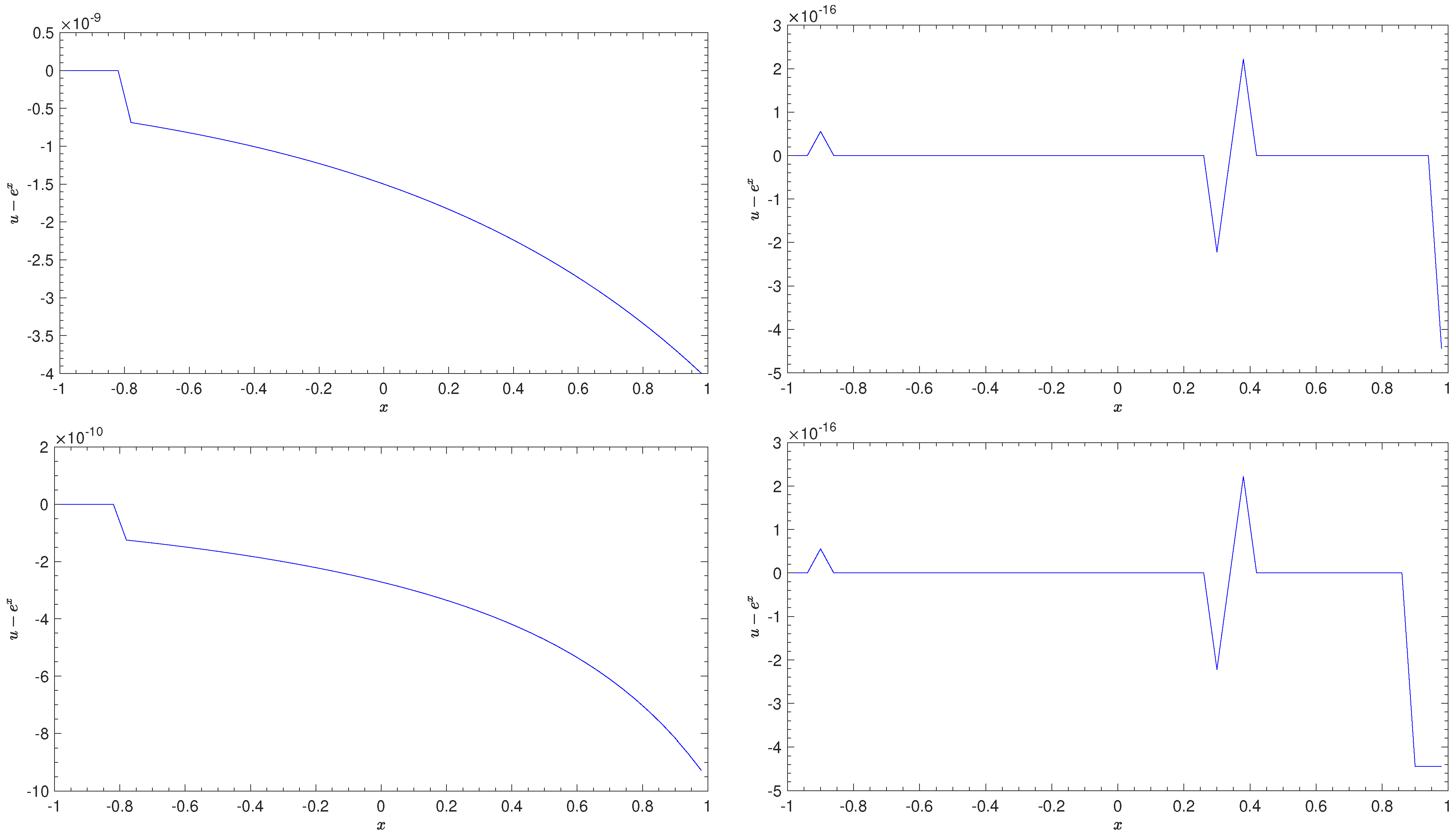
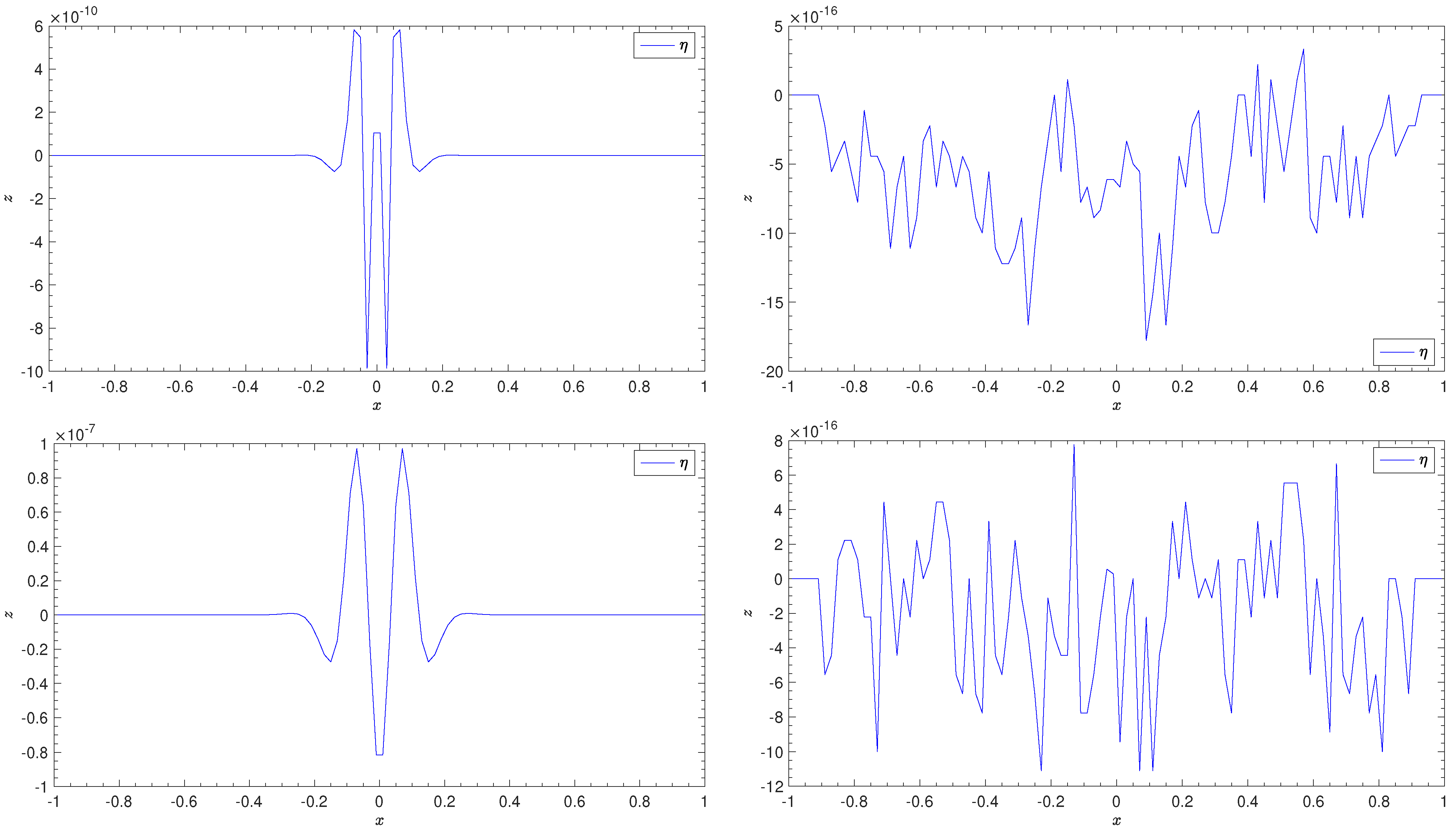
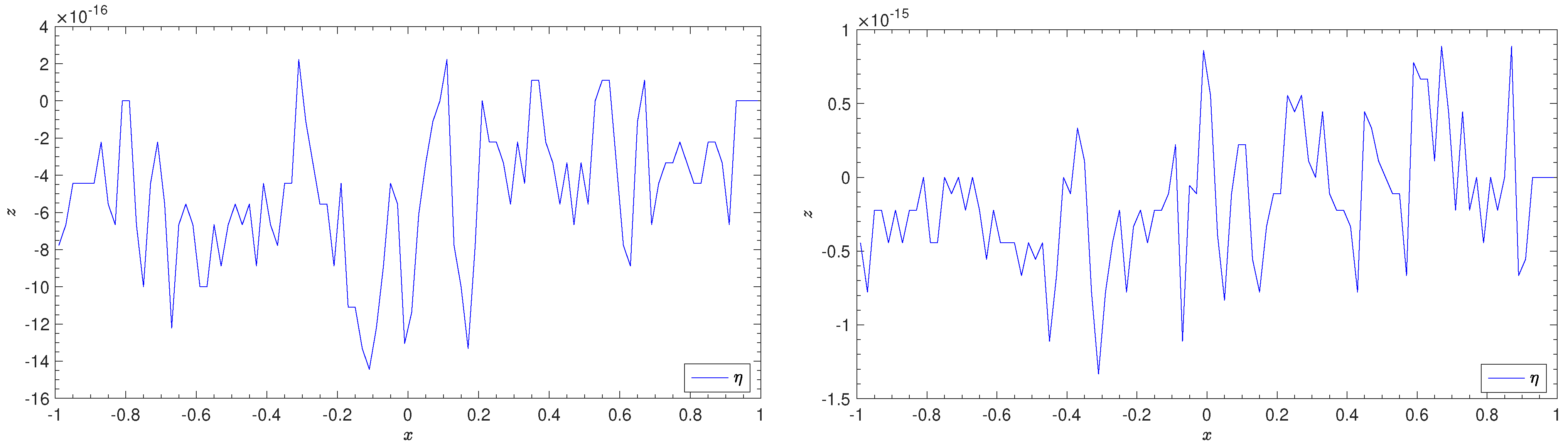
The computational domain is Dirichlet and open boundary conditions were imposed at the left and at the right of the domain, respectively. Figure 1 shows the error between the computed numerical solutions and the stationary one given by . As it can be seen in Figure 1 and Table 1, the well-balanced methods can preserve the stationary solution at a final time s.
5.1.2. Perturbed Stationary Solutions
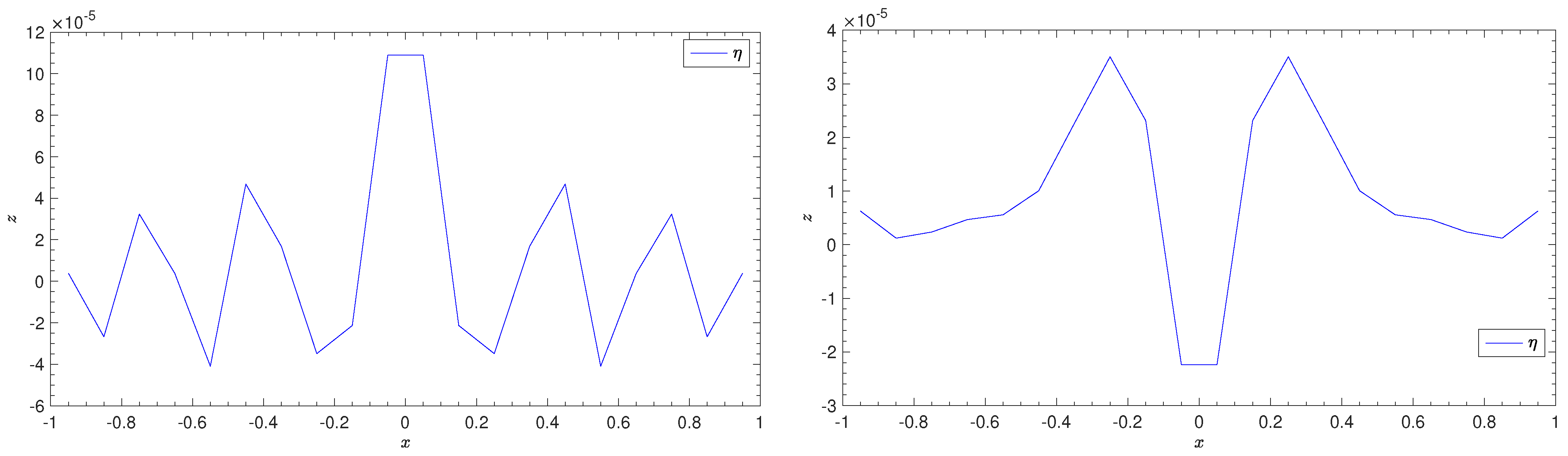
We consider now a perturbation of the stationary solution (44) given by
The computational domain is covered with a coarse mesh of elements. Dirichlet and open boundary conditions are imposed at the left and the right of the domain, respectively. The numerical experiment is run up to time s with the fourth-order DG method and for both Runge–Kutta and ADER time discretisations.
Figure 2 shows the error between the computed numerical solutions and the stationary one given by . As it can be seen, once the perturbation has left the domain, the well-balanced numerical scheme is able to recover the stationary solution , in contrast with the non well-balanced scheme.
5.1.3. Limited Simulation
In this final example, we aim to check the robustness of the proposed limiter technique described in this paper. To do that, we consider the initial condition
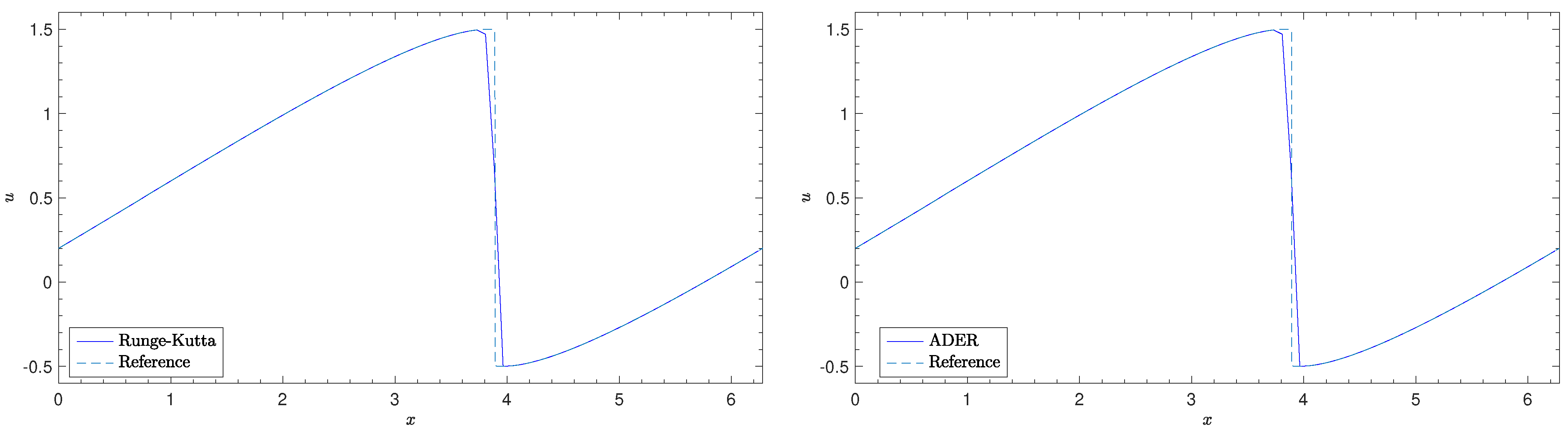
The computational domain is covered with a coarse mesh of elements. Periodic boundary conditions were imposed everywhere. Figure 3 shows the numerical approximation of u with different time-marching discretisations at the final time s, as well as a reference solution that has been computed by a first order scheme with 20,000 elements. As it can be seen, the proposed schemes provide an accurate approximation without producing any spurious oscillations, even for the case of coarse meshes.
5.1.4. Well-Balanced and Non-Well-Balanced Schemes Comparison
We perform now a comparison between the well-balanced and non-well-balanced schemes for a solution which is not a perturbation of an equilibrium state. Particularly, the following initial condition is considered:
Periodic boundary conditions and 100 discretization points are considered in a computational domain . Figure 4 depicts the results for a Runge–Kutta second and third order scheme. The reference solution has been computed using a first order method with 20,000 discretization points. As it can be seen, the results shows that the well-balanced and non well-balanced methods are in fact very similar regardless of the order of the method. Similar results are obtained for ADER time marching methods.
5.2. Shallow Water Equations
Let us consider the one-dimensional shallow water equations written in the form (1) with
where is the total water depth, u is the depth-averaged velocity on the -direction, and is the known still water depth that we will suppose to be continuous. Finally, is the gravitational acceleration. In this case we adapt the well-balanced strategy described in Section 3 to preserve the stationary solutions corresponding to water at rest:
where is the free-surface elevation.
A well-balance method could also be design following the ideas described in [93].
5.2.1. Order of Accuracy Test
We begin by checking numerically the order of accuracy of the numerical scheme for a Runge–Kutta and ADER time discretisation for a second-, third-, and fourth-order schemes. As pointed before, we consider here only a well-balanced method that preserves the water at rest solution adapting the strategy described in Section 3. The computational domain is , and periodic boundary conditions are imposed everywhere. We then simulate the propagation of a Gaussian wave, with the initial condition given by
and until the final time second, with a set of refined meshes. Table 2 shows the errors and the numerical convergence rates. The expected convergence order of the Runge–Kutta and ADER DG methods can be observed.
5.2.2. Preserving Stationary Solutions
In this experiment, we set as initial condition a stationary solution of the form (49) to ensure that the well-balanced methods are able to preserve it up to machine precision, while the non well-balanced methods fail. The initial condition considered is given by
The computational domain is and Dirichlet boundary conditions are imposed everywhere. As it can be seen in Figure 5 and Table 3 and Table 4, the well-balanced methods are able to preserve the stationary solution at a final time s for both time-marching discretisations and relative coarse meshes. Again, the numerical solutions are compared with the stationary solution (51) as reference.
5.2.3. Perturbed Stationary Solutions
We consider now a perturbation of the stationary solution (51) given by
The computational domain is covered with elements. Dirichlet and free-outflow boundary conditions are imposed at the right and the left of the domain, respectively.
As it can be seen in Figure 6, the well-balanced scheme can recover the stationary solution at a final time s with the fourth-order DG method and for both Runge–Kutta and ADER time discretisations. In this case, we plot the difference between the numerically computed free surfaces and the exact stationary (51), which is zero.
Moreover, in order to show the better performance of a well-balanced method against a non well-balanced method, we propose a similar numerical test on a very coarse mesh composed by 20 elements. Here, we consider the initial condition given by
The numerical computation is then run up to the short time s; the perturbation does not reach boundaries in this case, and therefore periodic boundary conditions were imposed everywhere.
As the perturbation is of the order , being the order of the scheme, we can expect that only the well-balanced method yields satisfactory results. In contrast, the non well-balanced scheme introduces oscillations of that order that destroy the solution. Here we only show the numerical results in Figure 7 for the Runge–Kutta time discretisation. Similar results can be observed for ADER time discretisations.
5.2.4. Limited Simulation
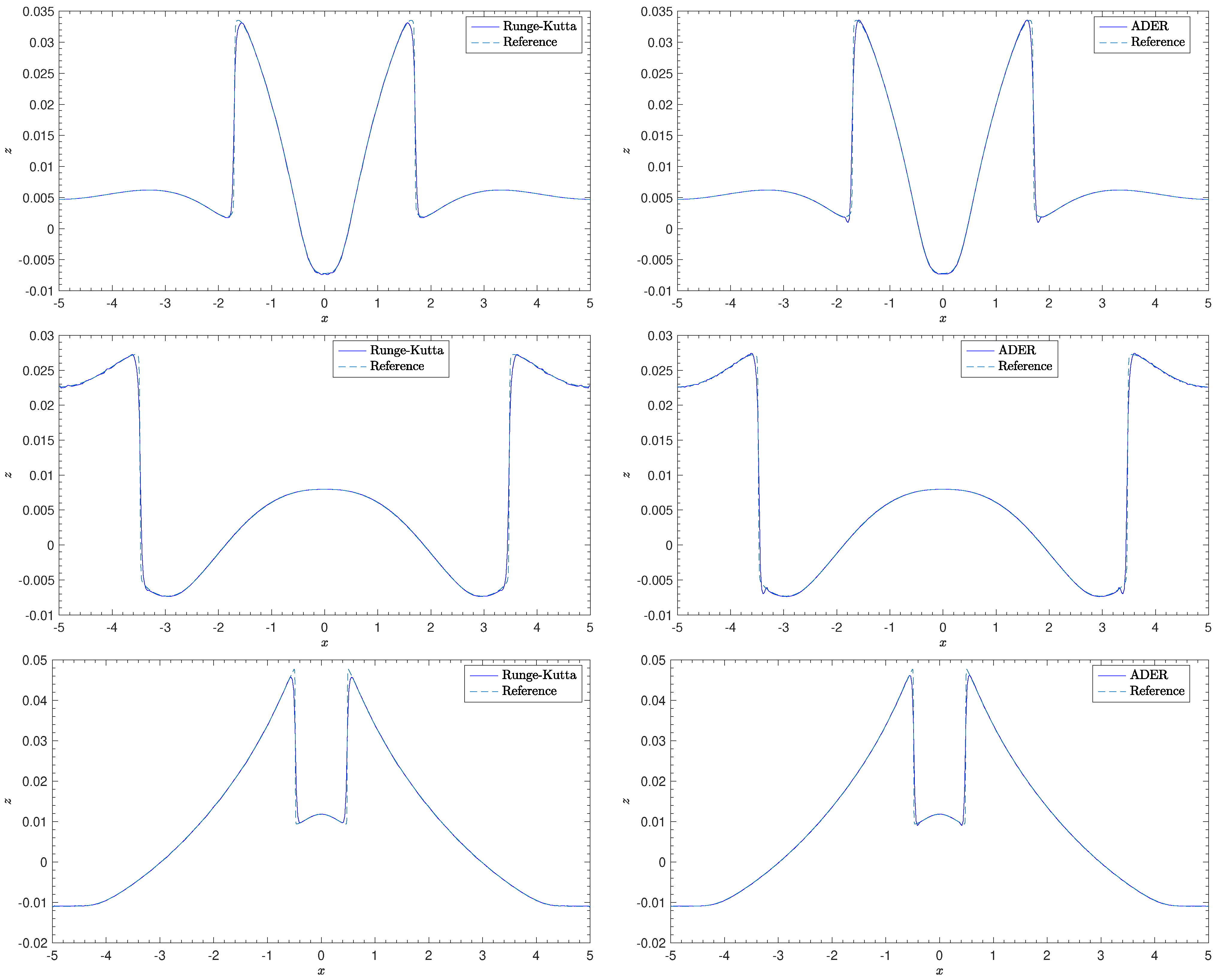
In order to check the robustness of the limiting procedure described in Section 4.3, we consider now a situation far from the equilibrium, where the use of some limiting technique is mandatory. The computational domain is covered now with a very refined mesh of elements. The initial condition is set to
Periodic boundary conditions are imposed to obtain more interactions between waves. Some snapshots of the computed free surface are depicted in Figure 8. As it can be observed, there are no oscillations at the neighbourhood of the shock waves, which indicates that the limiting approach provides a high overall quality of the computed numerical solution. The solution is depicted alongside a reference solution that has been computed by a first order scheme with 20,000 elements.
Note that the small oscillations appearing with the ADER method could be prevented with an ad hoc tuning of the parameters associated with the limiter described in Section 4. Here, we have maintained the same parameters for both approaches to compare both Runge–Kutta and ADER methods.
5.3. Compressible Euler Equations with Gravitational Force
We consider the gas dynamic Euler equations written as in (1):
being the density, u the velocity, E the total energy, and a given continuous gravitational potential. The internal energy e is given by . The pressure is given by e through the equation of state (ideal gas),
where is the adiabatic constant that will take the value unless stated otherwise.
In this work, we will focus on the hydrostatic steady states solutions given by
According to [35], a family of stationary solutions of (55) with are
where is a given continuous function and is given by
The numerical methods are then chosen to preserve one of those families given by the choice of
that results in the following set of stationary solutions with ,
5.3.1. Preserving Stationary Solutions
In this experiment, we set as initial condition a stationary solution of the form (60) to check the well-balancing properties of the proposed methods for the system (55). The initial condition is given by
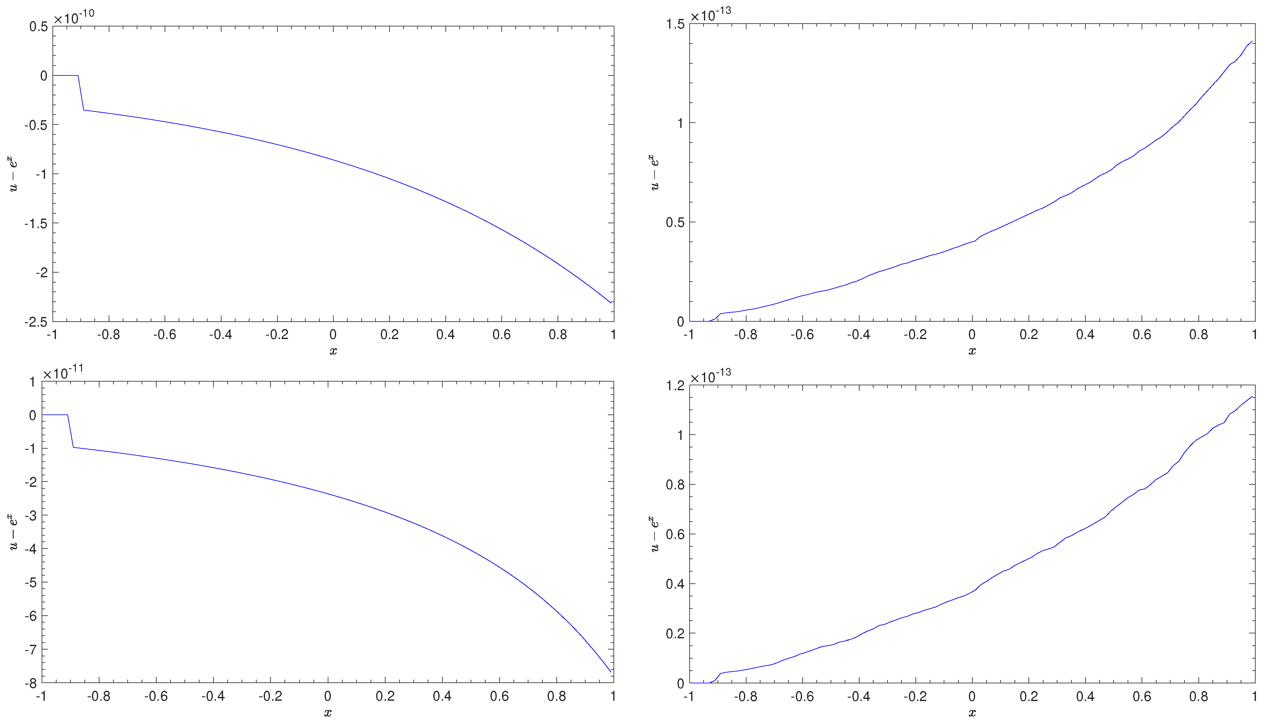
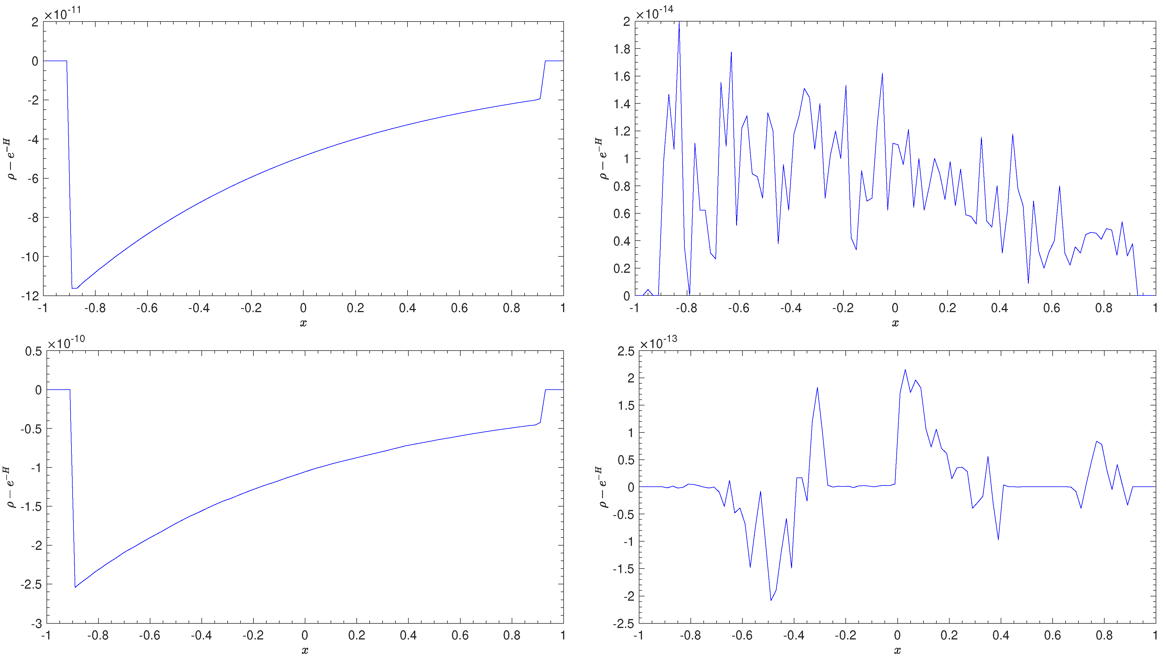
The computational domain is and Dirichlet boundary conditions were imposed everywhere. Figure 9 shows the error between the compute numerical solutions and the stationary one given by (61). As it can be seen in Figure 9 and Table 5, the well-balanced methods can preserve the stationary solution at a final time s.
5.3.2. Limited Simulation
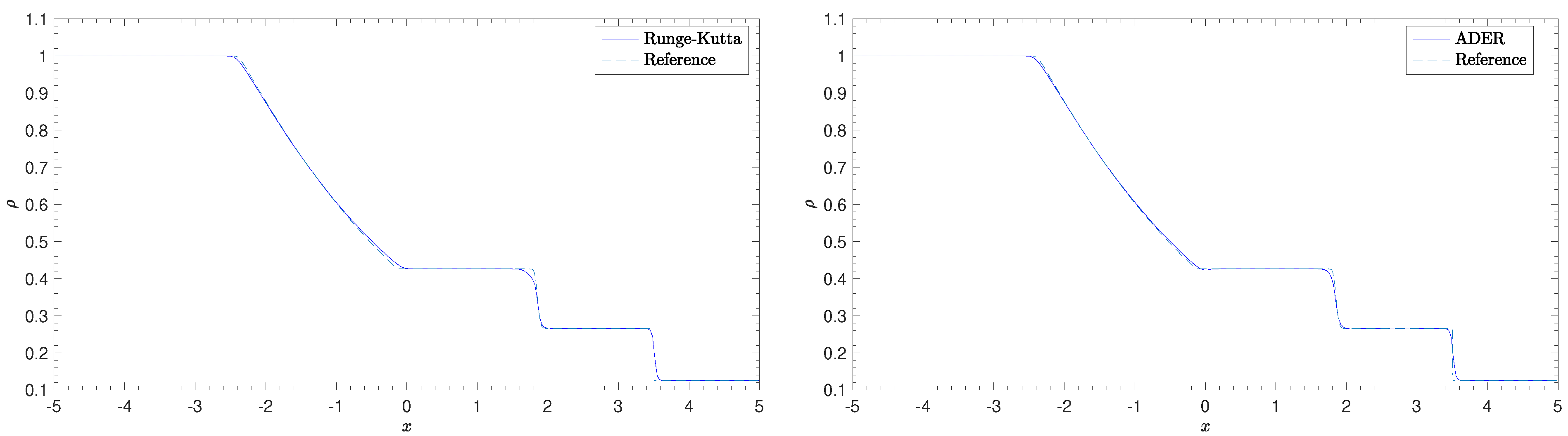
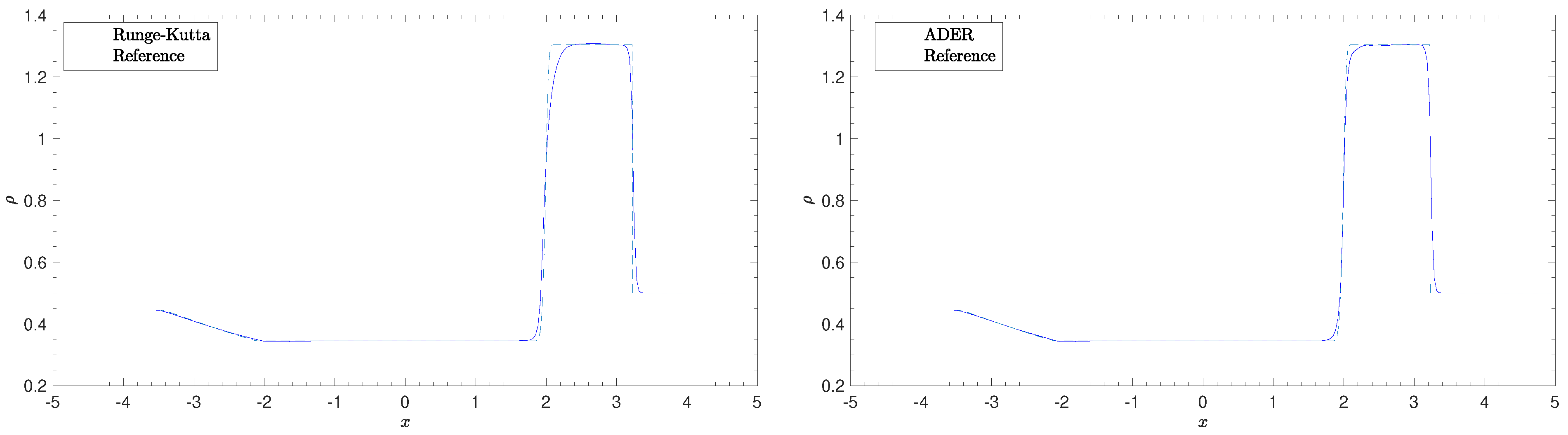
We check again the well behaviour of the proposed mixed-order technique described in this paper. To do that, we set and consider the following discontinuous initial condition given by
Then, we set the values for the two well-known numerical tests:
In both cases, the computational domain is covered with elements. The limiter value M defined in (33) is set to and the CFL number to Free outflow boundary conditions were imposed everywhere.
5.4. Dispersive Gavrilyuk–Favrie Equations
Finally, we will consider a hyperbolic dispersive shallow water system that was firstly introduced in [96] for the case of a flat bottom bathymetry, and later extended for the non-flat bottom case in [78]. The system can be seen as a hyperbolic relaxation approach of the elliptic Serre–Green–Naghdi equations, and is formally deduced from a master Lagrangian formalism. The system for the case of two-spatial domains reads
where
Here, is the water depth, is the known still water depth that we will assume to be continuous, and are the depth averaged velocities at the and z direction respectively. Furthermore, is the non-hydrostatic pressure
is the gravitational acceleration, and is a large pressure constant parameter that makes the system (66) formally converges to the elliptic Serre–Green–Naghdi equations [97] when Finally, is an auxiliary equilibrium variable introduced in the relaxation procedure. In the following, we will set for the numerical test considered.
The system satisfied an extra energy conservation law, and the eigenstructure is fully well known. For more details, the reader is refereed to [78]. As for Shallow-water equations, we will consider the family of stationary lake at rest solutions given by
where is the free-surface elevation.
There are many crucial reasons for considering the numerical validation of the proposed methods for that system here: we will validate the proposed numerical methodology for dispersive shallow flows numerical solutions, and the case of two spatial dimensions; the system introduces a non-homogeneous geometrical source term ; the usual steady-states lake at rest solutions for this system contains nonlinear relations between the conserved variables, and that makes standard well-balancing techniques no longer valid to preserve them. Finally, up to our knowledge, this is the first time that a well-balanced high-order method has been proposed for this particular dispersive hyperbolic system.
5.4.1. Preserving Stationary Solutions
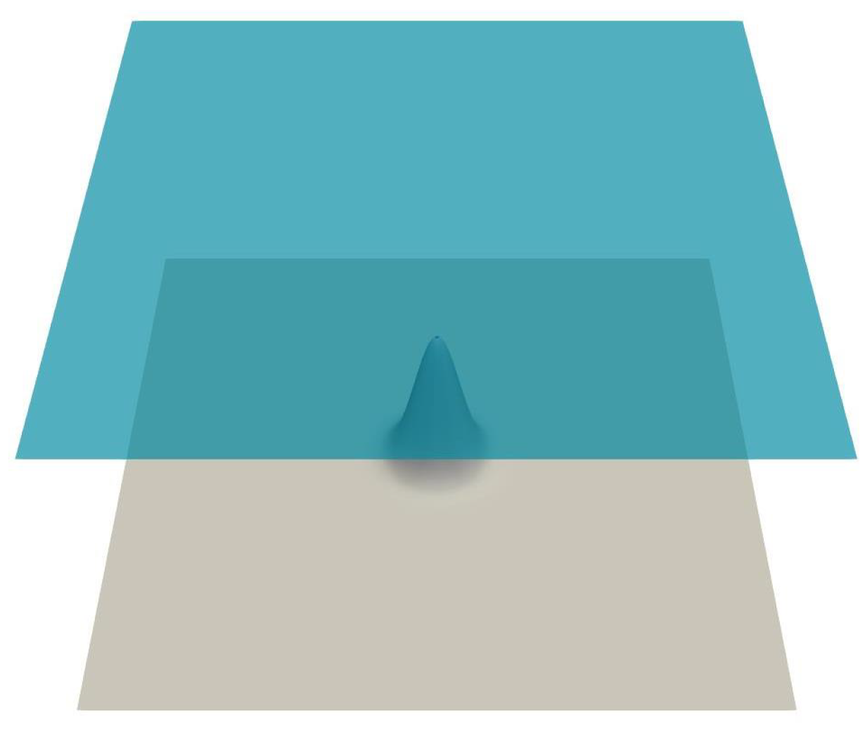
In this first numerical experiment, we set as initial condition a stationary solution of the form (67) to check the well-balancing abilities of the proposed methods for the system (66). The initial condition considered (see Figure 12) is given by
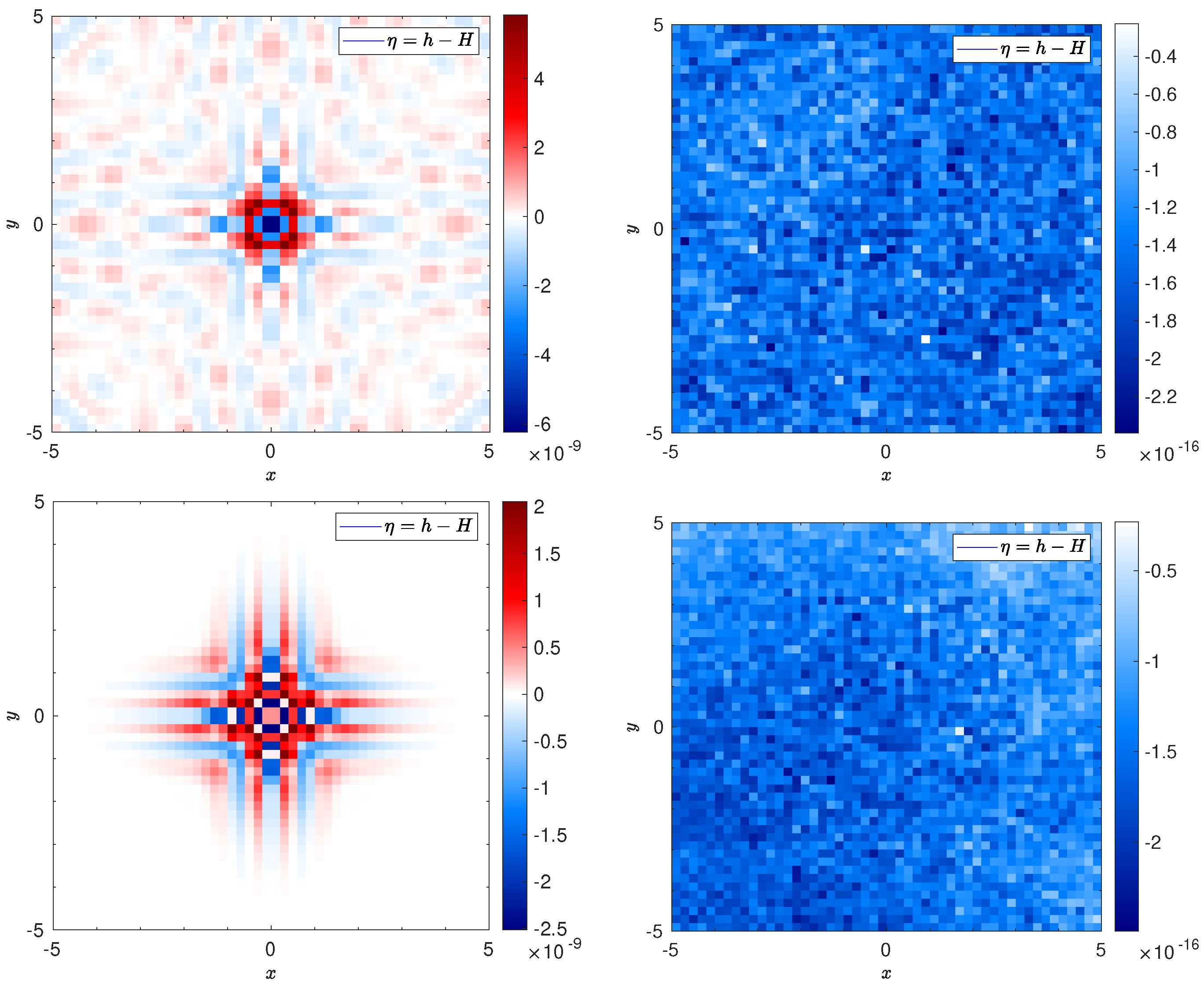
The computational domain is and periodic boundary conditions are imposed. As it can be seen in Figure 13 and Figure 14 and Table 6, the well-balanced methods are able to preserve the stationary solution at a final time s for both time-marching discretization and relative coarse meshes. Note that the solutions are compared against the stationary solution (68) as reference.
5.4.2. Limited Simulation
Next, we check the behaviour of the proposed mixed-order technique described in this paper. To do that, we set the following circular dam-break initial condition:
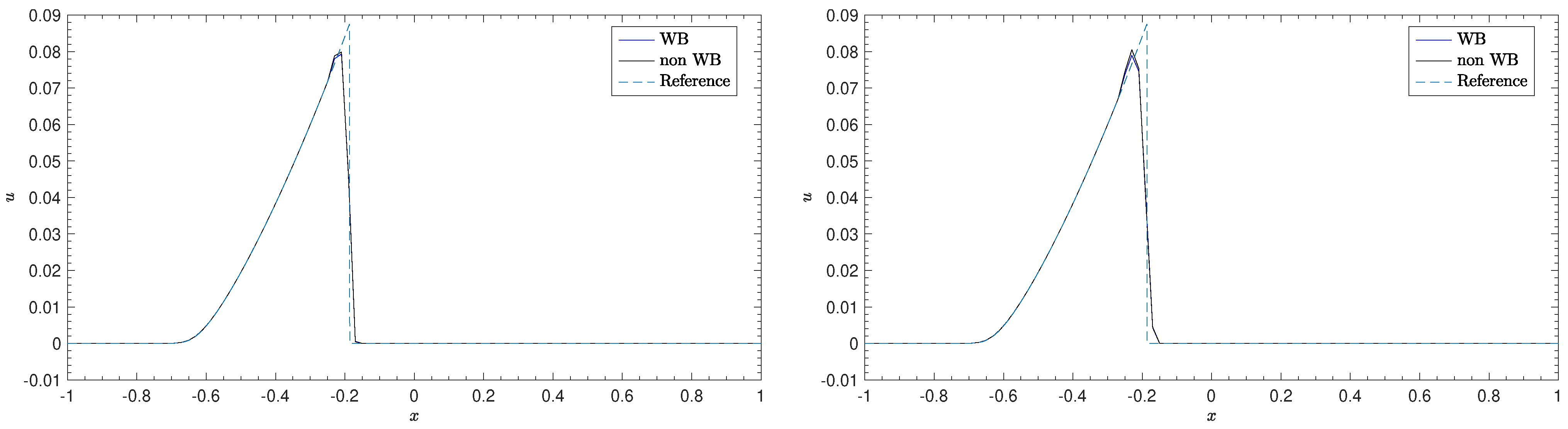
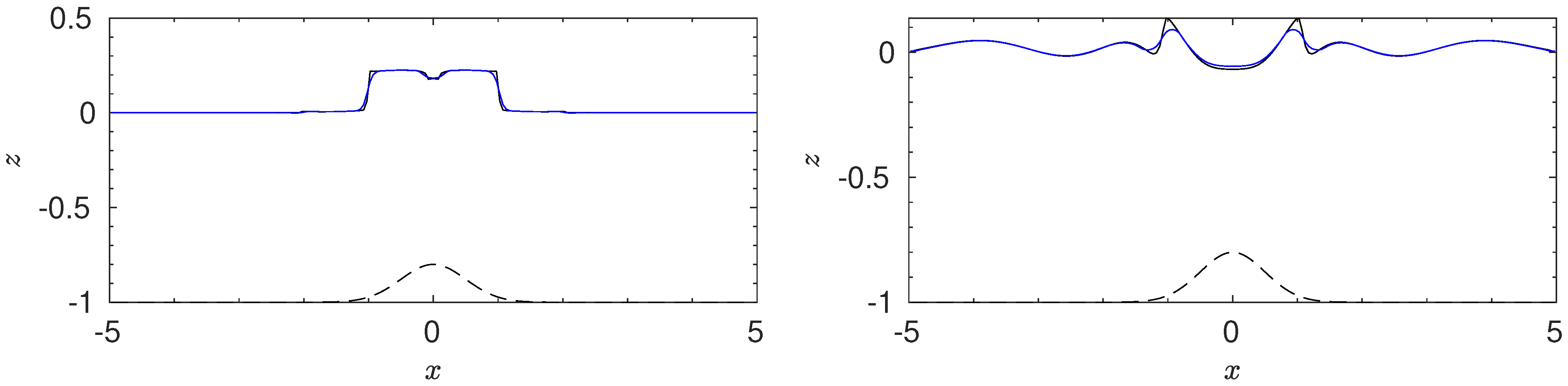
The computational domain is covered with a mesh of elements. We set periodic boundary conditions everywhere. Some snapshots of a section at of the computed free-surface are depicted in Figure 15 with a fourth-order Runge–Kutta time marching discretization. As it can be observed, the comparison between a limited and a non-limited simulation shows that there is no oscillations at the neighbourhood of the dispersive shock waves. Note that the high-oscillatory and over-amplified waves appearing in Figure 15 from the unlimited numerical solution, are not of the nature of this hyperbolic dispersive system.
6. Conclusions
We have presented a novel and general technique for preserving stationary solutions for Discontinuous Galerkin methods. This general approach is able to transform standard DG schemes in exactly well-balanced arbitrary high-order Discontinuous Galerkin methods for both Runge–Kutta and ADER time-marching discretisations.
For continuous source terms, the methodology only uses a well-suited definition of a well-balanced reconstruction operator and not on the Riemann-solver. Therefore, the well-balanced technique does not rely on the particular details of the system. That makes the method very general and can be applied to any system of hyperbolic PDEs, as long as the desired stationary solutions to be maintained are known.
Furthermore, the standard WENO limiting procedure is carefully considered. Here, we extend classical ideas to propose a novel WENO limiter that preserve stationary solutions. That makes the final numerical methods proposed here arbitrary high-order, essentially non-oscillatory and well-balanced.
We have tested the numerical methodology derived here with some standard systems, proving the well-balancing properties of the approach, the high-order accuracy, and the general well behaviour of the technique in the presence of strong discontinuities.
Author Contributions
Conceptualisation, M.J.C.D., C.E., and E.G.F.; methodology, C.E. and E.G.F.; software, C.E. and E.G.F.; validation, E.G.F. and C.E.; formal analysis, M.J.C.D., E.G.F., and C.E.; investigation, E.G.F., C.E., and M.J.C.D.; resources, M.J.C.D., E.G.F., and C.E.; data curation, C.E. and E.G.F.; writing—original draft preparation, E.G.F. and C.E.; writing—review and editing, M.J.C.D., C.E., and E.G.F.; visualisation, E.G.F. and C.E.; supervision, M.J.C.D.; project administration, M.J.C.D.; funding acquisition, M.J.C.D. All authors have read and agreed to the published version of the manuscript.
Funding
This research has been partially supported by the Spanish Government and FEDER through the coordinated Research project RTI2018-096064-B-C1, the Junta de Andalucía research project P18-RT-3163, the Junta de Andalucia-FEDER-University of Málaga research project UMA18-FEDERJA-16 and the University of Málaga. The University of Málaga has partially supported this research through the “Contrato Puente”.
Institutional Review Board Statement
Not applicable.
Informed Consent Statement
Not applicable.
Data Availability Statement
The code and datasets employed in the current paper are available from the authors on reasonable request.
Conflicts of Interest
The authors declare no conflict of interest.
References
- Bermúdez, A.; Vázquez, M.E. Upwind methods for hyperbolic conservation laws with source terms. Comput. Fluids 1994, 23, 1049–1071. [Google Scholar] [CrossRef]
- Audusse, E.; Bouchut, F.; Bristeau, M.O.; Klein, R.; Perthame, B. A fast and stable well-balanced scheme with hydrostatic reconstruction for shallow water flows. SIAM J. Sci. Comput. 2004, 25, 2050–2065. [Google Scholar] [CrossRef]
- Berberich, J.P.; Chandrashekar, P.; Klingenberg, C. High order well-balanced finite volume methods for multi-dimensional systems of hyperbolic balance laws. Comput. Fluids 2021, 219, 104858. [Google Scholar] [CrossRef]
- Guerrero Fernández, E.; Castro-Díaz, M.J.; Luna, T.M.d. A Second-Order Well-Balanced Finite Volume Scheme for the Multilayer Shallow Water Model with Variable Density. Mathematics 2020, 8, 848. [Google Scholar] [CrossRef]
- Bermúdez, A.; López, X.; Vázquez-Cendón, M.E. Finite volume methods for multi-component Euler equations with source terms. Comput. Fluids 2017, 156, 113–134. [Google Scholar] [CrossRef]
- Bouchut, F. Nonlinear Stability of Finite Volume Methods for Hyperbolic Conservation Laws: And Well-Balanced Schemes for Sources; Springer Science & Business Media: Berlin/Heidelberg, Germany, 2004. [Google Scholar]
- Brufau, P.; Vázquez-Cendón, M.; García-Navarro, P. A numerical model for the flooding and drying of irregular domains. Int. J. Numer. Methods Fluids 2002, 39, 247–275. [Google Scholar] [CrossRef]
- Canestrelli, A.; Siviglia, A.; Dumbser, M.; Toro, E.F. Well-balanced high-order centred schemes for non-conservative hyperbolic systems. Applications to shallow water equations with fixed and mobile bed. Adv. Water Resour. 2009, 32, 834–844. [Google Scholar] [CrossRef]
- Castro Díaz, M.J.; Chacón Rebollo, T.; Fernández-Nieto, E.D.; Parés, C. On Well-Balanced Finite Volume Methods for Nonconservative Nonhomogeneous Hyperbolic Systems. SIAM J. Sci. Comput. 2007, 29, 1093–1126. [Google Scholar] [CrossRef] [Green Version]
- Chacón Rebollo, T.; Domínguez Delgado, A.; Fernández Nieto, E.D. A family of stable numerical solvers for the shallow water equations with source terms. Comput. Methods Appl. Mech. Eng. 2003, 192, 203–225. [Google Scholar] [CrossRef]
- Chacón Rebollo, T.; Delgado, A.; Fernández-Nieto, E. Asymptotically balanced schemes for non-homogeneous hyperbolic systems—Application to the Shallow Water equations. Comptes Rendus Math. 2004, 338, 85–90. [Google Scholar] [CrossRef]
- Chandrashekar, P.; Zenk, M. Well-balanced nodal discontinuous Galerkin method for Euler equations with gravity. J. Sci. Comput. 2017, 71, 1062–1093. [Google Scholar] [CrossRef] [Green Version]
- Desveaux, V.; Zenk, M.; Berthon, C.; Klingenberg, C. A well-balanced scheme to capture non-explicit steady states in the Euler equations with gravity. Int. J. Numer. Methods Fluids 2016, 81, 104–127. [Google Scholar] [CrossRef]
- Desveaux, V.; Zenk, M.; Berthon, C.; Klingenberg, C. Well-balanced schemes to capture non-explicit steady states: Ripa model. Math. Comput. 2016, 85, 1571–1602. [Google Scholar] [CrossRef]
- Gaburro, E.; Castro, M.J.; Dumbser, M. Well-balanced Arbitrary-Lagrangian-Eulerian finite volume schemes on moving nonconforming meshes for the Euler equations of gas dynamics with gravity. Mon. Not. R. Astron. Soc. 2018, 477, 2251–2275. [Google Scholar] [CrossRef] [Green Version]
- Gaburro, E.; Castro, M.J.; Dumbser, M. A well balanced diffuse interface method for complex nonhydrostatic free surface flows. Comput. Fluids 2018, 175, 180–198. [Google Scholar] [CrossRef] [Green Version]
- Gaburro, E.; Dumbser, M.; Castro, M.J. Direct Arbitrary-Lagrangian-Eulerian finite volume schemes on moving nonconforming unstructured meshes. Comput. Fluids 2017, 159, 254–275. [Google Scholar] [CrossRef] [Green Version]
- Gosse, L. A well-balanced flux-vector splitting scheme designed for hyperbolic systems of conservation laws with source terms. Comput. Math. Appl. 2000, 39, 135–159. [Google Scholar] [CrossRef] [Green Version]
- Gosse, L. A well-balanced scheme using non-conservative products designed for hyperbolic systems of conservation laws with source terms. Math. Model. Methods Appl. Sci. 2001, 11, 339–365. [Google Scholar] [CrossRef] [Green Version]
- Gosse, L. Localization effects and measure source terms in numerical schemes for balance laws. Math. Comput. 2002, 71, 553–582. [Google Scholar] [CrossRef] [Green Version]
- Greenberg, J.; Leroux, A.; Baraille, R.; Noussair, A. Analysis and approximation of conservation laws with source terms. SIAM J. Numer. Anal. 1997, 34, 1980–2007. [Google Scholar] [CrossRef]
- Greenberg, J.M.; LeRoux, A.Y. A well-balanced scheme for the numerical processing of source terms in hyperbolic equations. SIAM J. Numer. Anal. 1996, 33, 1–16. [Google Scholar] [CrossRef]
- Grosheintz-Laval, L.; Käppeli, R. High-order well-balanced finite volume schemes for the Euler equations with gravitation. J. Comput. Phys. 2019, 378, 324–343. [Google Scholar] [CrossRef] [Green Version]
- Käppeli, R.; Mishra, S. Well-balanced schemes for the Euler equations with gravitation. J. Comput. Phys. 2014, 259, 199–219. [Google Scholar] [CrossRef]
- LeVeque, R.J. Balancing Source Terms and Flux Gradients in High-Resolution Godunov Methods: The Quasi-Steady Wave-Propagation Algorithm. J. Comput. Phys. 1998, 146, 346–365. [Google Scholar] [CrossRef] [Green Version]
- Noelle, S.; Pankratz, N.; Puppo, G.; Natvig, J.R. Well-balanced finite volume schemes of arbitrary order of accuracy for shallow water flows. J. Comput. Phys. 2006, 213, 474–499. [Google Scholar] [CrossRef]
- Noelle, S.; Xing, Y.; Shu, C.W. High-order well-balanced finite volume WENO schemes for shallow water equation with moving water. J. Comput. Phys. 2007, 226, 29–58. [Google Scholar] [CrossRef]
- Pelanti, M.; Bouchut, F.; Mangeney, A. A Roe-type scheme for two-phase shallow granular flows over variable topography. ESAIM Math. Model. Numer. Anal. Modélisation Mathématique Anal. Numérique 2008, 42, 851–885. [Google Scholar] [CrossRef] [Green Version]
- Perthame, B.; Simeoni, C. A kinetic scheme for the Saint-Venant system with a source term. Calcolo 2001, 38, 201–231. [Google Scholar] [CrossRef]
- Perthame, B.; Simeoni, C. Convergence of the upwind interface source method for hyperbolic conservation laws. In Hyperbolic Problems: Theory, Numerics, Applications; Springer: Berlin/Heidelberg, Germany, 2003; pp. 61–78. [Google Scholar]
- Gómez-Bueno, I.; Castro, M.J.; Parés, C. High-order well-balanced methods for systems of balance laws: A control-based approach. Appl. Math. Comput. 2021, 394, 125820. [Google Scholar] [CrossRef]
- Tang, H.; Tang, T.; Xu, K. A gas-kinetic scheme for shallow-water equations with source terms. Z. Angew. Math. Phys. ZAMP 2004, 55, 365–382. [Google Scholar] [CrossRef]
- Touma, R.; Koley, U.; Klingenberg, C. Well-balanced unstaggered central schemes for the Euler equations with gravitation. SIAM J. Sci. Comput. 2016, 38, B773–B807. [Google Scholar] [CrossRef]
- Müller, L.O.; Parés, C.; Toro, E.F. Well-balanced high-order numerical schemes for one-dimensional blood flow in vessels with varying mechanical properties. J. Comput. Phys. 2013, 242, 53–85. [Google Scholar] [CrossRef]
- Castro, M.J.; Parés, C. Well-balanced high-order finite volume methods for systems of balance laws. J. Sci. Comput. 2020, 82, 48. [Google Scholar] [CrossRef]
- Parés, C.; Parés-Pulido, C. Well-balanced high-order finite difference methods for systems of balance laws. J. Comput. Phys. 2021, 425, 109880. [Google Scholar] [CrossRef]
- Reed, W.H.; Hill, T. Triangular Mesh Methods for the Neutron Transport Equation; Technical Report; Los Alamos Scientific Lab.: Los Alamos, NM, USA, 1973. [Google Scholar]
- Cockburn, B.; Hou, S.; Shu, C.W. The Runge-Kutta Local Projection Discontinuous Galerkin Finite Element Method for Conservation Laws. IV: The Multidimensional Case. Math. Comput. 1990, 54, 545–581. [Google Scholar]
- Cockburn, B.; Lin, S.Y.; Shu, C.W. TVB Runge-Kutta local projection discontinuous Galerkin finite element method for conservation laws III: One-dimensional systems. J. Comput. Phys. 1989, 84, 90–113. [Google Scholar] [CrossRef] [Green Version]
- Cockburn, B.; Shu, C.W. TVB Runge-Kutta Local Projection Discontinuous Galerkin Finite Element Method for Conservation Laws II: General Framework. Math. Comput. 1989, 52, 411–435. [Google Scholar]
- Cockburn, B.; Shu, C.-W. The Runge-Kutta local projection P1-discontinuous-Galerkin finite element method for scalar conservation laws. ESAIM: M2AN 1991, 25, 337–361. [Google Scholar] [CrossRef]
- Xing, Y.; Zhang, X.; Shu, C.W. Positivity-preserving high order well-balanced discontinuous Galerkin methods for the shallow water equations. Adv. Water Resour. 2010, 33, 1476–1493. [Google Scholar] [CrossRef]
- Xing, Y. Exactly well-balanced discontinuous Galerkin methods for the shallow water equations with moving water equilibrium. J. Comput. Phys. 2014, 257, 536–553. [Google Scholar] [CrossRef]
- Xing, Y.; Shu, C.W. High order finite difference WENO schemes with the exact conservation property for the shallow water equations. J. Comput. Phys. 2005, 208, 206–227. [Google Scholar] [CrossRef]
- Xing, Y.; Shu, C.W. High Order Well-Balanced Finite Volume WENO Schemes and Discontinuous Galerkin Methods for a Class of Hyperbolic Systems with Source Terms. J. Comput. Phys. 2006, 214, 567–598. [Google Scholar] [CrossRef]
- Xing, Y.; Shu, C.W.; Noelle, S. On the Advantage of Well-Balanced Schemes for Moving-Water Equilibria of the Shallow Water Equations. J. Sci. Comput. 2011, 48, 339–349. [Google Scholar] [CrossRef] [Green Version]
- Bollermann, A.; Noelle, S.; Lukacova-Medvidova, M. Finite volume evolution Galerkin methods for the shallow water equations with dry beds. Commun. Comput. Phys. 2010, 10. [Google Scholar] [CrossRef] [Green Version]
- Xing, Y.; Zhang, X. Positivity-preserving well-balanced discontinuous Galerkin methods for the shallow water equations on unstructured triangular meshes. J. Sci. Comput. 2013, 57, 19–41. [Google Scholar] [CrossRef]
- Li, G.; Xing, Y. Well-balanced discontinuous Galerkin methods for the Euler equations under gravitational fields. J. Sci. Comput. 2016, 67, 493–513. [Google Scholar] [CrossRef]
- Li, G.; Xing, Y. Well-balanced discontinuous Galerkin methods with hydrostatic reconstruction for the Euler equations with gravitation. J. Comput. Phys. 2018, 352, 445–462. [Google Scholar] [CrossRef]
- Ern, A.; Piperno, S.; Djadel, K. A well-balanced Runge–Kutta discontinuous Galerkin method for the shallow-water equations with flooding and drying. Int. J. Numer. Methods Fluids 2008, 58, 1–25. [Google Scholar] [CrossRef] [Green Version]
- Vater, S.; Beisiegel, N.; Behrens, J. A limiter-based well-balanced discontinuous Galerkin method for shallow-water flows with wetting and drying: One-dimensional case. Adv. Water Resour. 2015, 85, 1–13. [Google Scholar] [CrossRef]
- Gassner, G.J.; Winters, A.R.; Kopriva, D.A. A well balanced and entropy conservative discontinuous Galerkin spectral element method for the shallow water equations. Appl. Math. Comput. 2016, 272, 291–308. [Google Scholar] [CrossRef] [Green Version]
- Taube, A.; Dumbser, M.; Balsara, D.S.; Munz, C.D. Arbitrary high-order discontinuous Galerkin schemes for the magnetohydrodynamic equations. J. Sci. Comput. 2007, 30, 441–464. [Google Scholar] [CrossRef]
- Dumbser, M.; Munz, C.D. Building blocks for arbitrary high order discontinuous Galerkin schemes. J. Sci. Comput. 2006, 27, 215–230. [Google Scholar] [CrossRef]
- Qiu, J.; Dumbser, M.; Shu, C.W. The discontinuous Galerkin method with Lax–Wendroff type time discretizations. Comput. Methods Appl. Mech. Eng. 2005, 194, 4528–4543. [Google Scholar] [CrossRef]
- Tumolo, G.; Bonaventura, L.; Restelli, M. A semi-implicit, semi-Lagrangian, p-adaptive discontinuous Galerkin method for the shallow water equations. J. Comput. Phys. 2013, 232, 46–67. [Google Scholar] [CrossRef]
- Dumbser, M.; Casulli, V. A staggered semi-implicit spectral discontinuous Galerkin scheme for the shallow water equations. Appl. Math. Comput. 2013, 219, 8057–8077. [Google Scholar] [CrossRef]
- Tavelli, M.; Dumbser, M. A high order semi-implicit discontinuous Galerkin method for the two dimensional shallow water equations on staggered unstructured meshes. Appl. Math. Comput. 2014, 234, 623–644. [Google Scholar] [CrossRef]
- Busto, S.; Tavelli, M.; Boscheri, W.; Dumbser, M. Efficient high order accurate staggered semi-implicit discontinuous Galerkin methods for natural convection problems. Comput. Fluids 2020, 198, 104399. [Google Scholar] [CrossRef] [Green Version]
- Titarev, V.; Toro, E. ADER: Arbitrary high order godunov approach. J. Sci. Comput. 2002, 17, 609–618. [Google Scholar] [CrossRef]
- Toro, E.; Titarev, V. Solution of the generalized Riemann problem for advection-reaction equations. Proc. R. Soc. A Math. Phys. Eng. Sci. 2002, 458, 271–281. [Google Scholar] [CrossRef]
- Titarev, V.; Toro, E. ADER schemes for three-dimensional non-linear hyperbolic systems. J. Comput. Phys. 2005, 204, 715–736. [Google Scholar] [CrossRef]
- Toro, E.; Titarev, V. Derivative Riemann solvers for systems of conservation laws and ADER methods. J. Comput. Phys. 2006, 212, 150–165. [Google Scholar] [CrossRef]
- Dumbser, M.; Enaux, C.; Toro, E.F. Finite volume schemes of very high order of accuracy for stiff hyperbolic balance laws. J. Comput. Phys. 2008, 227, 3971–4001. [Google Scholar] [CrossRef]
- Dumbser, M.; Balsara, D.S.; Toro, E.F.; Munz, C.D. A unified framework for the construction of one-step finite volume and discontinuous Galerkin schemes on unstructured meshes. J. Comput. Phys. 2008, 227, 8209–8253. [Google Scholar] [CrossRef]
- Escalante, C.; de Luna, T.M.; Castro, M. Non-hydrostatic pressure shallow flows: GPU implementation using finite volume and finite difference scheme. Appl. Math. Comput. 2018, 338, 631–659. [Google Scholar] [CrossRef] [Green Version]
- Li, G.; Song, L.; Gao, J. High order well-balanced discontinuous Galerkin methods based on hydrostatic reconstruction for shallow water equations. J. Comput. Appl. Math. 2018, 340, 546–560. [Google Scholar] [CrossRef]
- Li, G.; Li, J.; Qian, S.; Gao, J. A well-balanced ADER discontinuous Galerkin method based on differential transformation procedure for shallow water equations. Appl. Math. Comput. 2021, 395, 125848. [Google Scholar] [CrossRef]
- Wu, X.; Kubatko, E.J.; Chan, J. High-order entropy stable discontinuous Galerkin methods for the shallow water equations: Curved triangular meshes and GPU acceleration. Comput. Math. Appl. 2021, 82, 179–199. [Google Scholar] [CrossRef]
- Dumbser, M.; Castro, M.; Parés, C.; Toro, E.F. ADER schemes on unstructured meshes for nonconservative hyperbolic systems: Applications to geophysical flows. Comput. Fluids 2009, 38, 1731–1748. [Google Scholar] [CrossRef]
- Izem, N.; Seaid, M.; Wakrim, M. A discontinuous Galerkin method for two-layer shallow water equations. Math. Comput. Simul. 2016, 120, 12–23. [Google Scholar] [CrossRef]
- Wintermeyer, N.; Winters, A.R.; Gassner, G.J.; Warburton, T. An entropy stable discontinuous Galerkin method for the shallow water equations on curvilinear meshes with wet/dry fronts accelerated by GPUs. J. Comput. Phys. 2018, 375, 447–480. [Google Scholar] [CrossRef] [Green Version]
- Higdon, R.L. Discontinuous Galerkin methods for multi-layer ocean modeling: Viscosity and thin layers. J. Comput. Phys. 2020, 401, 109018. [Google Scholar] [CrossRef]
- Fernández, E.G.; Díaz, M.J.C.; Dumbser, M.; de Luna, T.M. An Arbitrary High Order Well-Balanced ADER-DG Numerical Scheme for the Multilayer Shallow-Water Model with Variable Density. J. Sci. Comput. 2021, 90, 52. [Google Scholar] [CrossRef]
- Escalante, C.; Dumbser, M.; Castro, M. An efficient hyperbolic relaxation system for dispersive non-hydrostatic water waves and its solution with high order discontinuous Galerkin schemes. J. Comput. Phys. 2019, 394, 385–416. [Google Scholar] [CrossRef]
- Bassi, C.; Bonaventura, L.; Busto, S.; Dumbser, M. A hyperbolic reformulation of the Serre-Green-Naghdi model for general bottom topographies. Comput. Fluids 2020, 212, 104716. [Google Scholar] [CrossRef]
- Busto Ulloa, S.; Dumbser, M.; Escalante, C.; Favrie, N.; Gavrilyuk, S. On high order ADER discontinuous galerkin schemes for first order hyperbolic reformulations of nonlinear dispersive systems. J. Sci. Comput. 2021, 87. [Google Scholar] [CrossRef]
- Dumbser, M.; Zanotti, O.; Loubère, R.; Diot, S. A posteriori subcell limiting of the discontinuous Galerkin finite element method for hyperbolic conservation laws. J. Comput. Phys. 2014, 278, 47–75. [Google Scholar] [CrossRef] [Green Version]
- Cockburn, B.; Shu, C.W. The Runge–Kutta Discontinuous Galerkin Method for Conservation Laws V: Multidimensional Systems. J. Comput. Phys. 1998, 141, 199–224. [Google Scholar] [CrossRef]
- Biswas, R.; Devine, K.D.; Flaherty, J.E. Parallel, adaptive finite element methods for conservation laws. Appl. Numer. Math. 1994, 14, 255–283. [Google Scholar] [CrossRef]
- Burbeau, A.; Sagaut, P.; Bruneau, C.H. A Problem-Independent Limiter for High-Order Runge–Kutta Discontinuous Galerkin Methods. J. Comput. Phys. 2001, 169, 111–150. [Google Scholar] [CrossRef]
- Zhong, X.; Shu, C.W. A simple weighted essentially nonoscillatory limiter for Runge–Kutta discontinuous Galerkin methods. J. Comput. Phys. 2013, 232, 397–415. [Google Scholar] [CrossRef]
- Qiu, J.; Shu, C.W. Runge–Kutta discontinuous Galerkin method using WENO limiters. SIAM J. Sci. Comput. 2005, 26, 907–929. [Google Scholar] [CrossRef]
- Shi, J.; Hu, C.; Shu, C.W. A technique of treating negative weights in WENO schemes. J. Comput. Phys. 2002, 175, 108–127. [Google Scholar] [CrossRef] [Green Version]
- Castro, M.; Fernández-Nieto, E. A Class of Computationally Fast First Order Finite Volume Solvers: PVM Methods. SIAM J. Sci. Comput. 2012, 34. [Google Scholar] [CrossRef] [Green Version]
- Castro, M.J.; de Luna, T.M.; Parés, C. Well-balanced schemes and path-conservative numerical methods. In Handbook of Numerical Analysis; Elsevier: Amsterdam, The Netherlands, 2017; Volume 18, pp. 131–175. [Google Scholar]
- Gallardo, J.M.; Schneider, K.A.; Castro, M.J. On a class of two-dimensional incomplete Riemann solvers. J. Comput. Phys. 2019, 386, 541–567. [Google Scholar] [CrossRef] [Green Version]
- Castro, M.J.; Gallardo, J.M.; Marquina, A. A class of incomplete Riemann solvers based on uniform rational approximations to the absolute value function. J. Sci. Comput. 2014, 60, 363–389. [Google Scholar] [CrossRef]
- Shu, C.W.; Osher, S. Efficient implementation of essentially non-oscillatory shock-capturing schemes. J. Comput. Phys. 1988, 77, 439–471. [Google Scholar] [CrossRef] [Green Version]
- Hidalgo, A.; Dumbser, M. ADER schemes for nonlinear systems of stiff advection–diffusion–reaction equations. J. Sci. Comput. 2011, 48, 173–189. [Google Scholar] [CrossRef]
- Jackson, H. On the eigenvalues of the ADER-WENO Galerkin predictor. J. Comput. Phys. 2017, 333, 409–413. [Google Scholar] [CrossRef]
- Castro Díaz, M.; López-García, J.; Parés, C. High order exactly well-balanced numerical methods for shallow water systems. J. Comput. Phys. 2013, 246, 242–264. [Google Scholar] [CrossRef]
- Sod, G.A. A survey of several finite difference methods for systems of nonlinear hyperbolic conservation laws. J. Comput. Phys. 1978, 27, 1–31. [Google Scholar] [CrossRef] [Green Version]
- Lax, P.D. Weak solutions of nonlinear hyperbolic equations and their numerical computation. Commun. Pure Appl. Math. 1954, 7, 159–193. [Google Scholar] [CrossRef]
- Favrie, N.; Gavrilyuk, S. A rapid numerical method for solving Serre–Green–Naghdi equations describing long free surface gravity waves. Nonlinearity 2017, 30, 2718. [Google Scholar] [CrossRef] [Green Version]
- Green, A.E.; Naghdi, P.M. A derivation of equations for wave propagation in water of variable depth. J. Fluid Mech. 1976, 78, 237–246. [Google Scholar] [CrossRef]
Figure 1.
Fluctuation for the stationary problem (44) for the Burgers’ equation at time s with the fourth order non well-balanced (left) and well-balanced (right) numerical schemes. An uniform Cartesian mesh of elements has been used. Upper and lower panels stands for Runge–Kutta and ADER time-marching discretisations, respectively.

Figure 2.
Fluctuation with respect to the stationary solution (45) for the Burgers’ equation at time s with the fourth order non well-balanced (left) and well-balanced (right) methods. An uniform Cartesian mesh of elements has been used. Upper and lower panels stands for Runge–Kutta and ADER time marching discretisations respectively.

Figure 3.
Computed variable u for the problem (46) (Burgers’ equation) with the fourth-order well-balanced Runge–Kutta (left) and ADER (right) numerical methods at time s. An uniform Cartesian mesh of elements has been used.
Figure 3.
Computed variable u for the problem (46) (Burgers’ equation) with the fourth-order well-balanced Runge–Kutta (left) and ADER (right) numerical methods at time s. An uniform Cartesian mesh of elements has been used.

Figure 4.
Computed variable u for the problem (47) (Burgers’ equation) with the second (left) and third (right) order well-balanced Runge–Kutta numerical methods at time s. An uniform Cartesian mesh of elements has been used.
Figure 4.
Computed variable u for the problem (47) (Burgers’ equation) with the second (left) and third (right) order well-balanced Runge–Kutta numerical methods at time s. An uniform Cartesian mesh of elements has been used.

Figure 5.
Computed free surface for the stationary problem (51) (sallow-water equations) at time s with the fourth order non well-balanced (left) and well-balanced (right) methods. An uniform Cartesian mesh of elements has been used. Upper and lower panels stands for Runge–Kutta and ADER time-marching discretisations respectively.

Figure 6.
Computed free surface of the perturbed stationary solution (52) (sallow-water equations) with the fourth order well-balanced Runge–Kutta (left) and ADER (right) DG schemes at s. A uniform Cartesian mesh of elements has been used.
Figure 6.
Computed free surface of the perturbed stationary solution (52) (sallow-water equations) with the fourth order well-balanced Runge–Kutta (left) and ADER (right) DG schemes at s. A uniform Cartesian mesh of elements has been used.

Figure 7.
Computed free surface of the smaller perturbed stationary solution (53) (sallow-water equations) with the fourth order non well-balanced (left) and well-balanced (right) Runge–Kutta DG method at s. A coarse uniform Cartesian mesh of elements has been used.
Figure 7.
Computed free surface of the smaller perturbed stationary solution (53) (sallow-water equations) with the fourth order non well-balanced (left) and well-balanced (right) Runge–Kutta DG method at s. A coarse uniform Cartesian mesh of elements has been used.

Figure 8.
Computed free surface for the problem (54) (shallow water equations) with the fourth-order well-balanced Runge–Kutta (left) and ADER (right) numerical methods at times s (from upper to lower panels). An uniform Cartesian mesh of elements has been used.
Figure 8.
Computed free surface for the problem (54) (shallow water equations) with the fourth-order well-balanced Runge–Kutta (left) and ADER (right) numerical methods at times s (from upper to lower panels). An uniform Cartesian mesh of elements has been used.

Figure 9.
Computed density variable fluctuation for the stationary problem (61) (Euler equations) at time s with the fourth order non well-balanced (left) and well-balanced (right) methods. An uniform Cartesian mesh of elements has been used. Upper and lower panels stands for Runge–Kutta and ADER time-marching discretisations, respectively.

Figure 10.
Computed density variable for the problem (63) (Euler equations) with the fourth-order well-balanced Runge–Kutta (left) and ADER (right) numerical methods at time s. An uniform Cartesian mesh of elements has been used.
Figure 10.
Computed density variable for the problem (63) (Euler equations) with the fourth-order well-balanced Runge–Kutta (left) and ADER (right) numerical methods at time s. An uniform Cartesian mesh of elements has been used.

Figure 11.
Computed density variable for the problem (64) (Euler equations) with the fourth-order well-balanced Runge–Kutta (left) and ADER (right) numerical methods at time s. An uniform Cartesian mesh of elements has been used.
Figure 11.
Computed density variable for the problem (64) (Euler equations) with the fourth-order well-balanced Runge–Kutta (left) and ADER (right) numerical methods at time s. An uniform Cartesian mesh of elements has been used.

Figure 12.
Bottom and the initial lake at rest free surface condition for the stationary problem (68) (dispersive Gavrilyuk–Favrie equations).
Figure 12.
Bottom and the initial lake at rest free surface condition for the stationary problem (68) (dispersive Gavrilyuk–Favrie equations).

Figure 13.
Computed free surface for the stationary problem (68) (dispersive Gavrilyuk–Favrie equations) at time s with the fourth-order non-well-balanced (left) and well-balanced (right) methods. A uniform Cartesian mesh of elements has been used. Upper and lower panels stands for Runge–Kutta and ADER time-marching discretisations, respectively.

Figure 14.
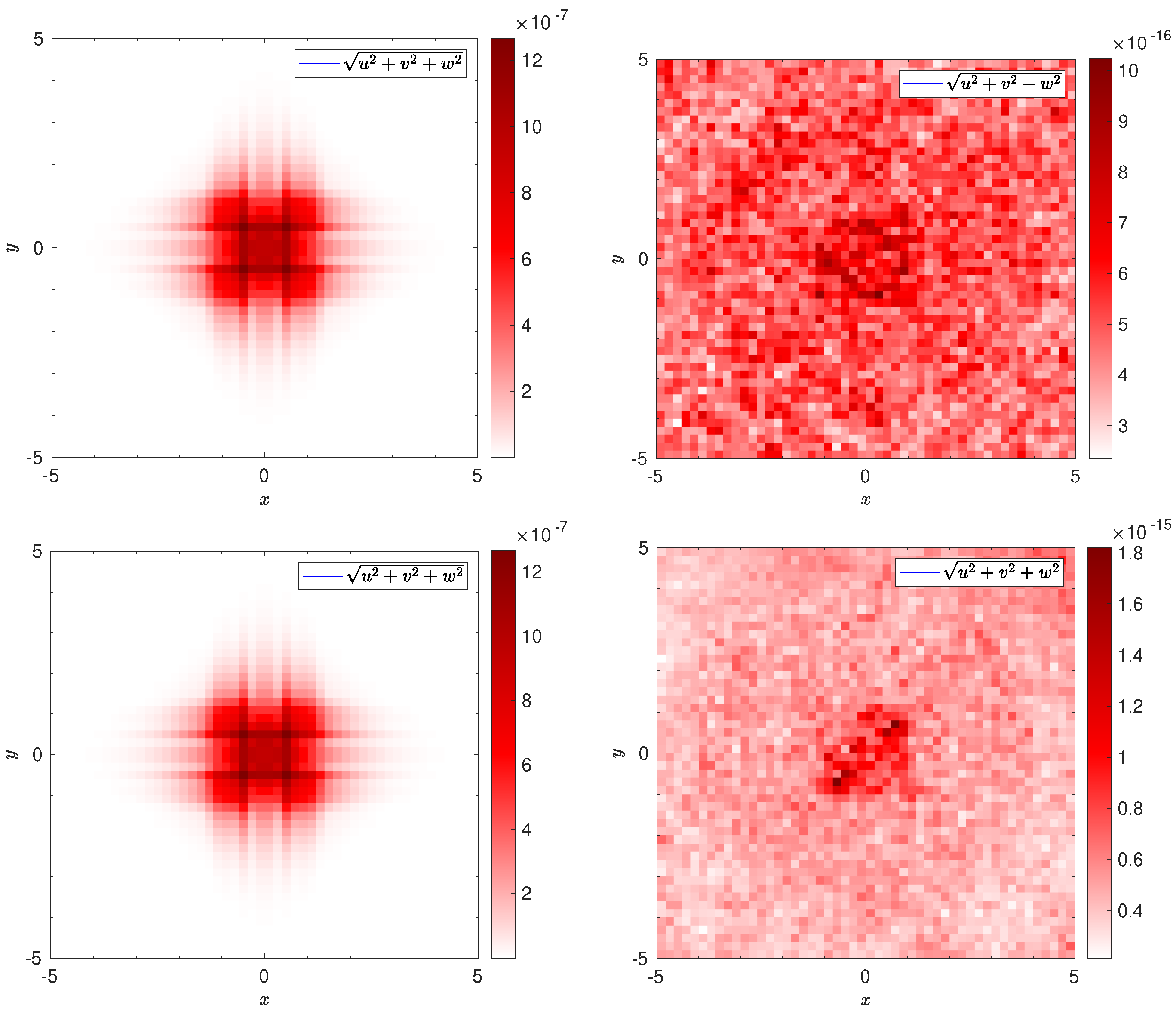
Computed velocity norm for the stationary problem (68) (dispersive Gavrilyuk–Favrie equations) at time s with the fourth order non well-balanced (left) and well-balanced (right) methods. An uniform Cartesian mesh of elements has been used. Upper and lower panels stands for Runge–Kutta and ADER time-marching discretisations, respectively.
Figure 14.
Computed velocity norm for the stationary problem (68) (dispersive Gavrilyuk–Favrie equations) at time s with the fourth order non well-balanced (left) and well-balanced (right) methods. An uniform Cartesian mesh of elements has been used. Upper and lower panels stands for Runge–Kutta and ADER time-marching discretisations, respectively.

Figure 15.
Cross section at of the computed free-surface for the problem (69) (dispersive Gavrilyuk–Favrie equations) at time s (left) and s (right) with the fourth order limited (blue) and non-limited (black) Runge–Kutta DG method. A uniform Cartesian mesh of elements has been used. Dashed lines stand for the bottom topography


Table 1.
Numerical validation of the well-balanced and non well-balanced methods for the stationary problem (44) (Burgers’ equation). Table contains errors for the variable u at a final time s for both Runge–Kutta and ADER DG schemes of order Uniform Cartesian meshes of elements has been used.
Table 1.
Numerical validation of the well-balanced and non well-balanced methods for the stationary problem (44) (Burgers’ equation). Table contains errors for the variable u at a final time s for both Runge–Kutta and ADER DG schemes of order Uniform Cartesian meshes of elements has been used.
| Non Well-Balanced | Well-Balanced | ||||
|---|---|---|---|---|---|
| N | Runge-Kutta | ADER | Runge-Kutta | ADER | |
| 0 | 25 | 0 | 0 | ||
| 50 | 0 | ||||
| 100 | 0 | ||||
| 200 | 0 | 0 | |||
| 1 | 25 | 0 | |||
| 50 | 0 | 0 | |||
| 100 | |||||
| 200 | |||||
| 2 | 25 | 0 | |||
| 50 | 0 | ||||
| 100 | 0 | ||||
| 200 | |||||
| 3 | 25 | ||||
| 50 | |||||
| 100 | |||||
| 200 | |||||
Table 2.
Numerical convergence results for the initial condition (50) (shallow water equations). High-order Runge–Kutta and ADER DG schemes of order Uniform Cartesian meshes of elements has been used. The errors refer to the variables h and at a final time s.
Table 2.
Numerical convergence results for the initial condition (50) (shallow water equations). High-order Runge–Kutta and ADER DG schemes of order Uniform Cartesian meshes of elements has been used. The errors refer to the variables h and at a final time s.
| Runge-Kutta | ADER | ||||||||
|---|---|---|---|---|---|---|---|---|---|
| Error | Order | Error | Order | Error | Order | Error | Order | ||
| 1 | 25 | - | - | - | |||||
| 50 | |||||||||
| 100 | |||||||||
| 200 | |||||||||
| 2 | 25 | - | - | - | - | ||||
| 50 | |||||||||
| 100 | |||||||||
| 200 | |||||||||
| 3 | 25 | - | - | - | - | ||||
| 50 | 3.94 | ||||||||
| 100 | 3.96 | ||||||||
| 200 | 3.98 | ||||||||
Table 3.
Numerical validation of the well-balanced and non well-balanced methods for the stationary problem (51) (shallow water equations). Table contains errors for the water depth variable h at a final time s for Runge–Kutta and ADER DG schemes of order Uniform Cartesian meshes of elements has been used.
| Non-Well-Balanced | Well-Balanced | ||||
|---|---|---|---|---|---|
| N | Runge–Kutta | ADER | Runge-Kutta | ADER | |
| 0 | 25 | ||||
| 50 | |||||
| 100 | |||||
| 200 | |||||
| 1 | 25 | ||||
| 50 | |||||
| 100 | |||||
| 200 | |||||
| 2 | 25 | ||||
| 50 | |||||
| 100 | |||||
| 200 | |||||
| 3 | 25 | ||||
| 50 | |||||
| 100 | |||||
| 200 | |||||
Table 4.
Numerical validation of the well-balanced and non well-balanced methods for the stationary problem (51) (shallow water equations). Table contains errors for the conserved variable at a final time s for Runge–Kutta and ADER DG schemes of order Uniform Cartesian meshes of elements has been used.
| Non-Well-Balanced | Well-Balanced | ||||
|---|---|---|---|---|---|
| N | Runge–Kutta | ADER | Runge–Kutta | ADER | |
| 0 | 25 | ||||
| 50 | |||||
| 100 | |||||
| 200 | |||||
| 1 | 25 | ||||
| 50 | |||||
| 100 | |||||
| 200 | |||||
| 2 | 25 | ||||
| 50 | |||||
| 100 | |||||
| 200 | |||||
| 3 | 25 | ||||
| 50 | |||||
| 100 | |||||
| 200 | |||||
Table 5.
Numerical validation of the well-balanced and non well-balanced methods for the stationary problem (61) (Euler equations). Table contains errors for the density variable at a final time s for both Runge–Kutta and ADER DG schemes of order Uniform Castesian meshes of elements has been used.
Table 5.
Numerical validation of the well-balanced and non well-balanced methods for the stationary problem (61) (Euler equations). Table contains errors for the density variable at a final time s for both Runge–Kutta and ADER DG schemes of order Uniform Castesian meshes of elements has been used.
| Non-Well-Balanced | Well-Balanced | ||||
|---|---|---|---|---|---|
| N | Runge–Kutta | ADER | Runge–Kutta | ADER | |
| 0 | 25 | ||||
| 50 | |||||
| 100 | |||||
| 200 | |||||
| 1 | 25 | ||||
| 50 | |||||
| 100 | |||||
| 200 | |||||
| 2 | 25 | ||||
| 50 | |||||
| 100 | |||||
| 200 | |||||
| 3 | 25 | ||||
| 50 | |||||
| 100 | |||||
| 200 | |||||
Table 6.
Numerical validation of the well-balanced and non well-balanced methods for the stationary problem (68) (dispersive Gavrilyuk–Favrie equations). Table contains errors for the water depth variable h at a final time s for Runge–Kutta and ADER DG schemes of order Uniform Cartesian meshes of elements has been used.
| Non-Well-Balanced | Well-Balanced | ||||
|---|---|---|---|---|---|
| N | Runge–Kutta | ADER | Runge–Kutta | ADER | |
| 0 | 20 × 20 | 0 | 0 | ||
| 30 × 30 | 0 | 0 | |||
| 40 × 40 | 0 | 0 | |||
| 50 × 50 | 0 | 0 | |||
| 1 | 20 × 20 | 0 | 0 | ||
| 30 × 30 | |||||
| 40 × 40 | 0 | 0 | |||
| 50 × 50 | |||||
| 2 | 20 × 20 | 0 | 0 | ||
| 30 × 30 | |||||
| 40 × 40 | 0 | 0 | |||
| 50 × 50 | |||||
| 3 | 20 × 20 | 0 | 0 | ||
| 30 × 30 | |||||
| 40 × 40 | |||||
| 50 × 50 | |||||
Publisher’s Note: MDPI stays neutral with regard to jurisdictional claims in published maps and institutional affiliations. |
© 2021 by the authors. Licensee MDPI, Basel, Switzerland. This article is an open access article distributed under the terms and conditions of the Creative Commons Attribution (CC BY) license (https://creativecommons.org/licenses/by/4.0/).
Share and Cite
MDPI and ACS Style
Guerrero Fernández, E.; Escalante, C.; Castro Díaz, M.J. Well-Balanced High-Order Discontinuous Galerkin Methods for Systems of Balance Laws. Mathematics 2022, 10, 15. https://0-doi-org.brum.beds.ac.uk/10.3390/math10010015
AMA Style
Guerrero Fernández E, Escalante C, Castro Díaz MJ. Well-Balanced High-Order Discontinuous Galerkin Methods for Systems of Balance Laws. Mathematics. 2022; 10(1):15. https://0-doi-org.brum.beds.ac.uk/10.3390/math10010015
Chicago/Turabian StyleGuerrero Fernández, Ernesto, Cipriano Escalante, and Manuel J. Castro Díaz. 2022. "Well-Balanced High-Order Discontinuous Galerkin Methods for Systems of Balance Laws" Mathematics 10, no. 1: 15. https://0-doi-org.brum.beds.ac.uk/10.3390/math10010015
Note that from the first issue of 2016, this journal uses article numbers instead of page numbers. See further details here.