
Incorporating ‘Mortgage-Loan’ Contracts into an Agricultural Supply Chain Model under Stochastic Output


Business School, Hunan Normal University, Changsha 410081, China
*
Author to whom correspondence should be addressed.
Mathematics 2022, 10(1), 85; https://0-doi-org.brum.beds.ac.uk/10.3390/math10010085
Submission received: 20 November 2021
/
Revised: 22 December 2021
/
Accepted: 22 December 2021
/
Published: 27 December 2021
(This article belongs to the Special Issue Supply Chain Management and Mathematical Logistics)
Abstract
:This paper constructs an internal financing model in which the purchaser acts as the core leading enterprise to provide loans when the farmer has fixed assets as collateral. Numerical results show that the existence of fixed assets will increase the expected profit of the farmer, redistributing the risk and profit between the purchaser and the farmer. At the same time, the purchaser and the government are encouraged to provide more funds to the farmer with low value of its fixed assets, which will aid the overall return of the supply chain and the development of supply chain finance. In addition, under the framework of this model, the increase of agricultural production is beneficial to the farmer, not the purchaser. In the case of the same output level, we can alleviate this problem by selecting high-end agricultural products with high price elasticity of demand and high choking price so as to improve the profits of both purchaser and farmer.
1. Introduction
Supply chain has received a lot of attention from scholars since the 1980s [1]. The deeper reason for its development is that along with the globalization of trade, the world’s leading companies have outsourced their operations to reduce their costs. This move has formed the global industrial chain, bringing the concept of supply chain management with the leading companies at the core [2]. Baron used the expected utility function as the objective function of system decision making, studying the problem of optimal decision making in the framework of the newsboy model [3]. This type of research approach is also the main approach in existing supply chain studies. Pasternack proposed that in the context of the newsboy model, specific contractual arrangements can provide effective coordination of the operation of the supply chain [4]. On this basis, Cachon and Larivere developed a general framework for revenue sharing contracts. They compared it with traditional coordination contracts, exploring its performance and scope of application in depth [5], and concluded that the contract has better results. Based on the different economic backgrounds of each country, the development of enterprises in different countries has shown different focuses, which has also led to the enrichment and development of research related to supply chain management from different directions [6,7,8].
In the process of supply chain production, each production link is interdependent, and the shortcomings formed at any node will affect the overall efficiency of the supply chain [9]. At the end of the last century, entrepreneurs and scholars found that the capital constraint and financing cost of small and medium-sized enterprises are the key factors that restrict the development of the supply chain [10]. Financing is critical to the supply chain [11]. Specifically, there are two financing channels for SMEs. The first channel is collateral-based loans provided by banks, where the collateral is usually the supplier’s physical assets such as plant, equipment and inventory [12]. The second channel is factoring, where the supplier sells the receivables at a discount to the financial institution for immediate cash payment [13,14]. However, both channels require suppliers to have certain tangible internal resources, which may not be easily available. Thus, the exploration of the value of the financial supply chain has become a new area of interest. The supply chain finance, as a special financial model serving and relying on the supply chain, has gradually surfaced. Supply chain finance only provides targeted financial services to the participants in the supply chain. It can integrate and distribute the capital flow, commercial flow, logistics flow and information flow in the supply chain [15].
Most of the previous studies, which are based on a newsvendor model, analyze the interactions between production and financing decisions [16]. However, the academic community has not yet formed a unified definition of supply chain finance. Timme restricts supply chain finance to the scope where financial institutions participate, that is, the third-party financial institutions outside the supply chain provide financing services for participants in the supply chain [17]. Hoffmann sees supply chain finance as a coordination of financial resources among participants within the supply chain [18]. Through effective control, the value of capital can be added. Combining the above two mainstream discussions, existing studies have mostly integrated the two approaches within the framework of supply chain finance. It can be divided into two categories: external financing and internal financing [19]. One of the most common forms of external financing is known as purchase order financing (POF), in which financial institutions provide loans to suppliers based on purchase orders issued by reputable manufacturers in the supply chain. The providers of POF include traditional commercial banks and specialized POF lenders [20,21]. Unlike asset-based loans and factoring which require tangible assets as collateral, the repayment of POF loans is dependent on the successful delivery of the underlying purchase order by the supplier. Because POF loans are simply purchase orders issued by creditworthy buyers, the main risk associated with POF is not the credit risk of the buyer but the performance risk of the supplier [22]. The most representative endogenous financing is commercial credit, which allows the core company to relieve the financial pressure of the led party through advance payment or deferred collection [23]. Lamoureux and Evans made a new definition on the basis of previous research. They believe that supply chain finance integrates transaction information in the supply chain, and established a cost analysis framework for it [24]. Then, they sought the optimal financing model. Most of the existing studies are adding more realistic elements to the classical analytical framework. Deng et al. considered the influence of the green credit policy provided by the government on the decision variables of both sides in the game under the POF financing model [25]. It is argued that the government’s provision of green credit support along with enhanced regulation of the environment can lead to an increase in overall supply chain profits, and this initiative has a positive externality of environmental improvement. Yan et al., on the other hand, considered a three-stage supply chain model containing manufacturers, capital-constrained retailers, and banks that provide loans, and solved for the respective optimal performance in the Stackelberg game framework [26]. As the scope of the study continues to expand, the perspectives of the study become richer. Song et al. studied the profitability of different SMEs in supply chain finance by using strong connections and weak connections as the distinguishing point. In their empirical analysis, it is more detailed and deeper to use the sample data of 208 SMEs that have carried out supply chain financing services [27]. Fang and Xu investigates the financing options for a capital-constrained manufacturer when both green credit financing and mixed financing options were available [28].
The agricultural supply chain is a special branch of the supply chain, which is different from other industrial supply chains. Its special characteristics are determined by the role of agricultural products and the performance of the supply chain hosts and customers [29], and the reason is mainly from the high risk associated with the uncertainty of production in the agricultural industry. Uncertainty in agricultural production mainly refers to the fact that the output of agricultural products is often random due to uncertainties factors such as weather and seasons [30]. For agricultural product suppliers who invest a certain volume of agricultural materials, their actual output and expected output often have a certain difference. This is what we call the risk of output uncertainty. In the long term, the development of agriculture has been constrained by this risk. Therefore, many scholars have researched and discussed this issue. Wang and Gerchak earlier studied the problem of contract farming under the stochastic situation of output and demand, providing relevant suggestions for the optimal decision of contract farming [31]. Zant suggested that the default risk due to this output uncertainty can be effectively hedged by hedging in the futures market [32]. Bogetoft and Olesen argued that it is necessary to consider coordination, incentives, and transaction costs before designing contracts [33]. Allen and Schuster suggested a capacity optimization approach to manage and mitigate output uncertainty, while He and Zhang considered the risk sharing mechanism under stochastic output [34,35]. Therefore, they concluded that output stochasticity can improve supply chain performance. In order to reduce the overall operating cost of agriculture in the stochastic output scenario, the “company + farmers” model of contract farming is proposed to effectively reduce the blindness of farmers’ decision making. Through the rational decision making of the production parties, the stable operation of each production chain is ensured. It makes an important contribution to the improvement of the overall efficiency of the agricultural supply chain and the increase of farmers’ income [36]. Inderfurth and Vogelgesang studied supply chain coordination under output uncertainty [37]. Chen et al. systematically studied the supply chain situation of farmers constrained by funds under the output uncertainty, solving the optimization problem of purchasers and farmers [38]. Nong and Pang proposed a richer form of financing, which improves both the operability and the overall risk resistance of the supply chain from the perspective of enhancing flexibility [39]. Toole and Hennessy started to investigate the issue of the impact of subsidies on agricultural supply chains [40]. Huang and Lin further introduce an insurance mechanism in the presence of government subsidies based on the study of the risks associated with output uncertainty. They made the policy recommendation that government subsidies should always be provided in order to maximize social welfare [41]. As the research progresses, the direction of the study becomes more specific. Cai et al. studied the situation of a three-stage supply chain consisting of logistics suppliers, producers, and distributors. They consider the contractual choice of the three parties in the game to maximize their respective profits when the product is perishable [42]. On the basis of the same consideration of a three- stage supply chain, Bergeb et al. expand on the scope of risk. They explored financing under conditions of uncertainty in output, demand and market prices [43]. With the rapid development of the economic environment, existing studies have begun to introduce the impact of blockchain technology, COVID-19 and other factors on agricultural supply chains in different countries [44,45,46].
As can be seen, all of these studies have addressed the issue of financial constraints on farmers from the outside. None of them have considered that farmers can provide collateral to lenders to increase the probability of loan success. We believe that the existence of loan collateral actually provides a risk-sharing mechanism between the farmer and the lender. In the previous supply chain literature, there has not been much consideration of loan collateral and risk-sharing mechanism factors. When Kouvelis et al. studied the impact of different financing models on firms’ profits, they found that the value of collateral affects the level of their own profits when firms use external financing models [47]. Bai et al. have explored repurchase mechanisms based on inventory pledge financing supply chain coordination in their study on solving the financing problems of SMEs [48]. Lin et al. analyzed the impact of risk-sharing contracts under output uncertainty on the profitability of each party in the contract agricultural supply chain [49]. Nonetheless, the field of agricultural supply chain finance still considers less the situation where farmers have collateral.
This paper focuses on the introduction of the ‘mortgage-loan’ contractual model in traditional agricultural supply chain production and considers the implications of this model for all participants in the supply chain. The basic framework is to solve for the values of the decision variables that maximize the profit of the acquirer and the farmer in turn, using a sequential game in the context of intra-agricultural supply chain financing. Then, we liberalize the range of exogenous variables one by one to study the sensitivity analysis of exogenous variables on each decision quantity and the profit of both sides of the game, and reasonable policy recommendations are given accordingly. The model presented in this paper is a new exploration of risk-sharing mechanisms and therefore simplifies and ignores the impact of traditional risk-sharing approaches such as government subsidies and agricultural insurance. The model can therefore be optimally extended by continuing to include these traditional methods in subsequent studies.
The main contributions of this article can be summarized as follows:
- A new model of agricultural supply chain lending is proposed. This model assumes that the farmers have only fixed assets that can be used for production and that such fixed assets are pledged to obtain loans to purchase production materials. This is in fact a risk-sharing mechanism. It can promote the probability of loan success while effectively reducing the risk borne by the purchaser. It can also effectively reduce the moral hazard problem of farmers as they bear part of the responsibility for loan failure;
- In the absence of external financing, the purchaser will face both the wholesale price and the loan rate as two decision variables. Therefore, unlike the previous Stackelberg game where each level of the game process only determines one decision variable, the purchaser as the second level of the game will decide both the optimal wholesale price and the lending rate to maximize its own profit. This makes the model more realistic;
- In the numerical simulation section, we consider that the calculated optimal decision variables may not meet the realistic situation, such as the loan interest rate can be higher than the national allowed loan standard. It is also common for the loan amount to exceed the lending capacity of the purchaser. Therefore, we specify the range of values of each decision variable. We stipulate that the two sides of the game play within the range of values, so that the optimal decision will be a more realistic guidance.
2. The Model
2.1. The Model Construction
2.1.1. The Theoretical Framework and Variable Definitions
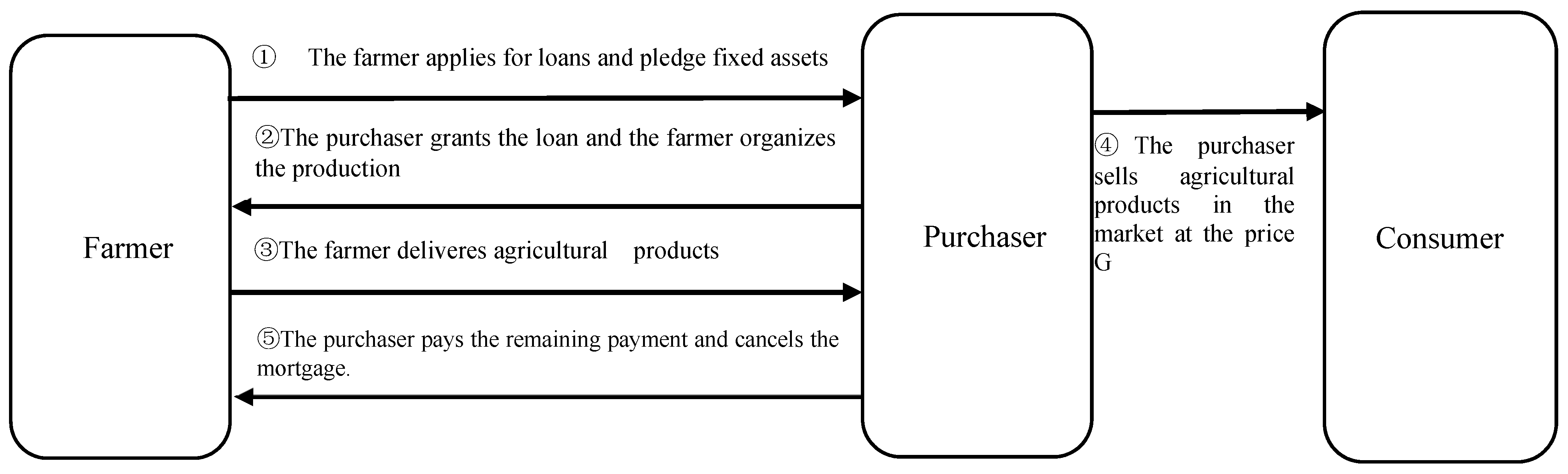
Here, we consider a two-level supply chain model. The model consists of a farmer who has fixed assets for production and a purchaser who purchases all the crops produced by the farmer, both of which are risk neutral and the purchaser is the core firm of the supply chain. In the first stage of production, the farmer faces a production capital shortage and needs to apply for a loan from the purchaser for production in that production period. The farmer can take the fixed assets used in production as collateral for the purchaser to apply for a loan with an interest rate of . After obtaining a loan that allows him to purchase production materials, farmer organize his production. At the end of a production cycle, the purchaser buys the produce and deducts the farmer’s loan. At this point a loan cycle ends.
Before constructing the model, we further make the following assumptions:
- Crop production is usually subject to a high degree of external uncertainty, such as the effects of climate, pests and other factors. We therefore use to represent the uncertain output, where is the uncertainty variable affecting output. The cumulative distribution function is , and the probability density function is , where ;
- At the end of the production period, the purchaser buys all the farmer’s produce at price and sells it on the market. For the sake of analysis, we use the assumption of equilibrium between supply and demand for agricultural products, i.e., the market is able to clear (). At this point the purchaser can sell all the produce at price G. Where , is the ratio of the purchase price set by the purchaser to the market price, then ;
- Reference to the setting of Cai et al. [42], we assume that the market for agricultural products is an elastic market. The price demand function can be expressed as , where is the inverse of the price elasticity of demand.
All parameters are set as shown in Table 1 below.
2.1.2. Discussion of Production Situation Classification
The purchaser completes all sales and pays the remaining amount to the farmer after deducting the principal and interest on the loan receivable. Because of the uncertainty of the farmer’s output, we can divide the results into two main categories of cases based on production and sales. In the first type of situation, the value of the payment delivered by the farmer to the purchaser is greater than the principal and interest of the loan. The purchaser pays the farmer normally and returns all the collateral to the farmer. The second type of situation is that the value of the loan is less than the principal and interest of the loan. At this time, it can be divided into two small cases. Specifically, in the first case, although the payment is less than the principal and interest of the loan, the difference is less than the farmer’s mortgage. Hence, the purchaser does not provide the farmer with the payment for products, but must return part of the mortgage. The second case is that the value of the purchase price plus the collateral is still less than the loan principal and interest. Now, the purchaser retains all the sales income and the collateral, but does not claim the remaining debt from the farmer. The timeline of this loan is shown in Figure 1:
2.1.3. The Utility Function
In the early stage of production, the farmers mortgage their fixed assets to the purchaser to obtain loan funds for production. The product will be delivered at the end of the production period, then the loan principal and interest will be repaid after the purchaser completes the sale. First, the sales income of farmers is , and is known from the market clearing conditions. From the above expressions of and , we can get . Therefore, the sales income of the farmer can be expressed as . In summary, the utility function of the farmer’s income is
After acquiring all the farmer’s products, the purchaser will sell them in the market. We have assumed that the purchaser will be able to sell all of the product at price G. Therefore, it can be concluded that part of the purchaser’s expected income comes from the sales profit, that is, the sales income minus the acquisition cost. Another part of the purchaser’s profit comes from the loan interest income. From the classification we discussed above, it’s not difficult to know that when the farmer can always repay the loan principal and interest normally, the purchaser’s income is , and if the farmer is still insufficient to repay the principal and interest of the loan with the mortgaged assets, the income of the purchaser will be . Therefore, the utility function of the purchaser can be expressed as
2.2. Optimal Solution
The Stackelberg game, proposed by H. Von Stackelberg, is a model for solving the optimal decision of each firm when there is asymmetric competition between the leader and the led firm [50]. The model takes into account the fact that there are leaders and leaders in the game, so it is widely used in solving problems related to supply chain management [51,52]. This paper is still based on the framework of the Stackelberg game and considers that the farmer and the purchaser make their decisions separately in a rule with game sequencing. The specific steps are as follows: the purchaser, as the core enterprise of the supply chain, has the dominant power to set the optimal loan rate and the optimal purchase price that can maximize its profit before the farmer’s decision. From the equation the purchase price is determined by the market price of agricultural products , and the purchase discount, which is expressed as the ratio of the purchase price to the market price . Considering that the price of agricultural products is determined by the market. Neither the farmer nor the purchaser has control over this variable. It can be considered as an exogenous variable in the model. Therefore, discussing the purchase price , one of the purchaser’s decision variables, can be equated to considering the ratio of the purchase price decided by the purchaser to the market price . On the basis of the purchaser’s decision, the farmer determine their own loan amount, and then they carry out the production according to the loan interest rate and the purchase price. In the case of a given production function, the optimal loan amount of farmer can be determined by using the principle of profit maximization. According to the characteristics of the Stackelberg game, the solution sequence should be as follows: assuming that the loan interest rate and the ratio of the purchase price to the market price are given, we can find the optimal loan amount and the optimal output of the farmer. The amount is a reaction function about the loan interest rate and the purchase price discount. Substituting the reaction function into the profit function of the core enterprise, we can solve the purchaser’s maximizing profit, and then the optimal loan interest rate and the optimal purchase price can be solved.
2.2.1. Solving for the Optimal Loan Amount
According to the described Stackelberg game, it is clear that there is a critical value of productivity that makes it impossible for the farmer to return the entire loan principal and interest even with the addition of fixed assets, which we set to . From this, inequalities can be established: . Thus, we can get
When is satisfied, the farmer can always repay the loan principal and interest at this time. The profit can be expressed as . When meets , the farmer will lose all collateral assets. From this, we can write the expression of the farmer’s expected return as
Therefore, the optimization problem for the farmer is
Regarding the optimal strategy of the farmer, we can obtain the following proposition.
Proposition 1.
Assume the farmer’s optimization problem is that we investigate the optimal loan amount in order to maximize the profit of the farmer. That is,
Then, the optimal loan amount for the farmer is given by:.
That is, when, the profit of the farmer reaches maximal value,
The proof of Proposition 1 is given in Appendix A.
The above equation is the optimal amount for the farmer, so there exists an optimal choice of loan amount for the farmer subject to a given loan interest rate. It is not difficult to conclude that the expression of contains the variable . Therefore, we call at this point a reaction function with respect to and .
2.2.2. Solving for the Purchaser’s Optimal Decision Variables
According to the Stackelberg game, the optimal interest rate and the purchase price set by the purchaser are based on the premise that the volume of the farmer’s loan is accurately predicted to be the optimal loan amount . In other words, the purchaser can obtain the farmer’s response function, making the optimal decision based on the response function. In the process of solving the optimal lending rate of the purchaser, all will be represented by .
It is known that a portion of the purchaser’s profit is derived from the sale of the product, and the expected profit of this portion can be expressed as
Another part of the profit comes from the interest income of the loan. So, from the above discussion, it is clear that the total expected return function of the purchaser is
The purchaser’s optimization problem is
Hence, the important proposition about the optimal decision of the purchaser is received as follows:
Proposition 2.
Suppose that the response function of the farmer is known. Assume that the purchaser’s optimization problem is that we choose the optimal interest rate r* and ratio of the optimal purchase price to the market price y* in order to maximize the purchaser’s profit. That is,
Then, the optimal interest rate r* and ratio of the optimal purchase price to the market price y* correspond to the solution of the following system of equations:
and
The proof of Proposition 2 is given in Appendix B.
Remark 1.
By using the joint cubic equation system, we can get the optimal loan rateand the optimal purchase price (where is determined by ) that should be set such that the purchaser’s profit is maximized. The specific numerical solution we will analyze by MATLAB software in the next section after substituting the corresponding parameters and setting the qualifying conditions that are consistent with the reality.
3. Numerical Analysis
In this section, we will use MATLAB software to find the optimal decision variables for the farmer and the purchaser by giving specific values that fit the actual situation. In addition, we will extend the range of exogenous variables to perform sensitivity analysis on the decision variables and profits of each party.
3.1. The Selection of Parameter Base Values
We prioritize the use of previous representative literature on the values of parameters in numerical arithmetic examples. We use these values as a basis for sensitivity analysis by expanding the range of values in the second subsection. According to Cai et al., we let and 0,000 [53]. With reference to Lin and Ye, we set obeys a uniform distribution of [54]. We refer to Chen et al. by fitting corn and early rice yield price data to obtain a setting of between 10 and 20, taking [38].
We conduct numerical simulations using the above-mentioned set of base parameters to find the values of the decision variables that maximize the profit of the farmer and the purchaser. At the same time, we restrict the range of decision variables in order to fit the actual situation, where , , . Figure 2a,b below shows the variation of profit of the purchaser and the farmer with their respective decision variables.
From the Stackelberg game, it is clear that the leading enterprise decides the decision variables first based on the profit maximization principle. Figure 2a shows a surface plot of the change in the purchaser’s profit with the ratio of the purchase price to the market price () and the loan interest rate (). We can see that there exists a point (, ) that makes the purchaser’s profit maximum. Substituting the optimal decision variables and of the purchaser into the profit function of the farmer, we can get the Figure 2b. It expresses the change in the profit of the farmer with the loan amount. We can see that the profit of the farmer is maximized when = 9.
Based on the above analysis, we can obtain a base result of the model as shown in Table 2.
3.2. Sensitivity Analysis for Changing Each Parameter
3.2.1. Expanding the Range of Values of Fixed Assets
According to the loan process, the farmer pledges the fixed assets that can be used for production to the purchaser. Then the purchaser issues the corresponding loan and determines the loan interest rate, the purchase price and some other variables. Therefore, the farmers’ fixed assets are not only the necessary tools for production, but also the basis for obtaining loans. However, the difference in the production of the farmer and the newness of the equipment may make the value of fixed assets available for mortgage different. In this section, we will present the detailed steps of conducting sensitivity analysis, and all subsequent sections will follow the method. First, we analyze how the two decision variables of the purchaser will change with the increase of fixed assets under the Stackelberg game. Next, we will analyze the trend of the loan amount of the farmer. Figure 3 represents the trend of the purchaser’s profit.
The purchaser’s profit plane represents the decision plane of the purchaser at different levels of . We can see that the purchaser’s profit plane sinks as the farmer’s fixed assets increase, that is say, the purchaser’s expected profit will be decreasing. In the selection of the optimal decision variables of the purchaser, points A1, A2 and A3 will be selected in turn. The corresponding values are , and . According to the Stackelberg’s sequence, we need to solve for the optimal decision variables of the farmer by substituting the purchaser’s decision variables into the profit function of the farmer with different values of . The change curve of farmer’s profit function is shown in Figure 4.
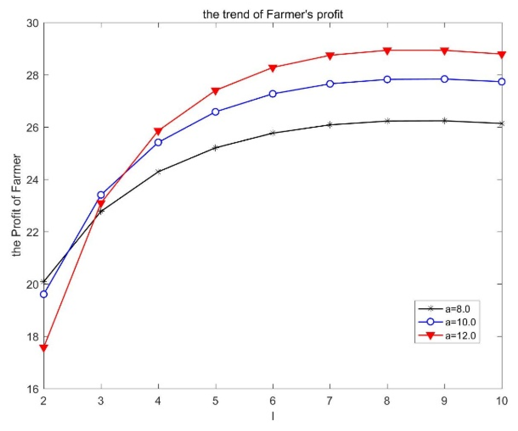
On top of the decision already made by the purchaser, the farmer’s decision remains to maximize profit. By observing Figure 4, we can see that among the three sets of values of above, the optimal decision of the farmer is all at , but with the increase of fixed assets , the optimal profit of the farmer is monotonically increasing. In order to analyze the changes more accurately, we need to increase the density of the fixed assets changes to further observe the trend of optimal profit of both parties. Figure 5 below represents the curve of the best profit of the farmer and the purchaser, as well as the change trend of each decision variable when the fixed asset increases from 80,000 by 25,000–120,000.
Figure 5a represents the trends in their respective optimal decision variables for both the purchaser and the farmer, where the coordinates of the left vertical axis in the figure represent the decision variables and of the purchaser and the coordinates of the right vertical axis represent the decision variables of the farmer. Figure 5b represents the trend of profit of the purchaser and the farmer respectively as increases. First, it can be seen that with the increase in fixed assets, the farmer’s optimal loan amount and the ratio of the purchaser’s purchase price to the market value do not change. Hence, the increase in the farmer’s fixed assets does not make the farmer expand production as a result, and because the low purchase price represents a strong bargaining position of the purchaser, the lower the purchase price the greater the profit margin the purchaser obtains. Hence, the increase in fixed assets alone does not prompt the purchaser to make concessions with other parameters remaining unchanged. Second, with the increase of fixed assets , the farmer’s profit will increase while the purchaser’s expected profit will decrease. The reason may be the fact that, as the fixed assets increase, the critical value of the farmer’s inability to return the loan properly will decrease. It is known from the previous analysis that the farmer does not increase the loan amount to expand production. Therefore, the moral hazard of inactive production by the farmer increases, and the risk to the purchaser increases. In addition, combined with the loan interest rate curve, it is found that an increase in interest rate will lead to an increase in the absolute value of the slope of the purchaser’s profit curve. In other words, the rate of decline in the purchaser’s profit has accelerated. It may because that the increase in loan interest rates has increased the pressure on farmers to repay the loans, thereby increasing the risk of the purchaser of recovering the principal and interest of the loan. This has led to a decline in the purchaser’s expected profit growth rate.
3.2.2. The Change of the Choking Price
The choking price, an exogenous variable in the model, is the maximum price at which the purchaser can sell the agricultural products in the product market. Although the final price of agricultural products will also be influenced by the market supply and demand, the choking price determines its upper limit. That will directly affect the profit of the farmer and the purchaser. Therefore, similar to the previous analysis, in this section we will expand the range of the choking price by increasing its value from 13 to 23 sequentially in 1-unit step. We use MATLAB to perform numerical simulations to obtain trend plots of the changes in each decision variable between the farmer and the purchaser.
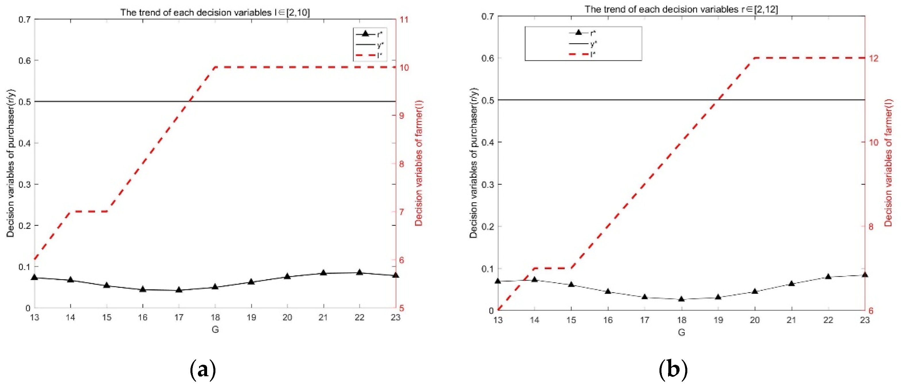
Figure 6a indicate the influence of the choking price on the purchaser’s optimal decision variable and the optimal loan amount for the farmer. It is not difficult to find that the ratio of the purchase price to the market price, which is one of the purchaser’s decision variables, has always remained unchanged at the level of . This is mainly because, as explained above, in order to make the model more in line with the actual situation, we limit the value range of the decision variable. In order to maximize its own profits, the purchaser will inevitably make the most beneficial choice. Therefore, no matter how the choking price changes, the lowest purchase price can enable the purchaser to obtain more benefits from the farmers without causing damage to itself. However, another decision variable of the purchaser will increase first and then decrease as the choking price increases. Combined with the analysis of the right-hand vertical axis in Figure 6a, which indicates the trend in the amount of loans to the farmer, we can conclude the reason. As the choking price rises, the profit that the purchaser and the farmer can obtain in the product market will increase. Furthermore, the probability that the farmer can repay the loans normally will increase. At this time, the purchaser is willing to lower the interest rate in order to allow the farmer to increase the loan amount and expand production. However, when the loan amount of farmer reaches the upper limit of the purchaser’s loan credit, it will be meaningless to reduce interest rates to stimulate farmers to increase loans. As the choking price continues to rise, the purchaser begins to increase the loan interest rate. The farmer is willing to maintain the original production scale, too. Based on the characteristics of the Stackelberg game, the purchaser can always judge the decisions of the farmer in advance. Hence, they will raise its loan interest rate. We know that the upper limit of the purchaser’s loan limit has hindered the growth of farmer’s optimal decision-making. Therefore, Figure 6b show that when we relax the upper limit of the loan limit, the lowest loan interest rate has shifted to the right. The optimal loan amount for the farmer has continued to rise to 120,000 with the increase in the choking price. Based on the changes in the above decision variables, we can analyze the profit curves of all parties, as shown in Figure 7.
Both the profit of the farmer and the purchaser are positively correlated with the choking price, which shows that the increase in the choking price can bring incremental benefits to both parties in the game. However, it can be seen that the effect of growth on both parties is not equal. There is a certain trade-off relationship between the growth rate of the farmer and the purchaser. Specifically, when is between 15 and 18, the purchaser’s profit grows the fastest, and is also the position where the optimal loan amount of the farmer appears inflection point. Therefore, the reason for the rapid growth of the initial profit of the purchaser is because it has benefited from the growth of the choking price and the expansion of the loan business volume. While a very important factor in the later profit slowdown comes from the stagnation of the growth of the loan amount of the farmer. Compared with Figure 7b, as the upper limit of the loan limit increases, the position of the purchaser’s profit slowdown has also shifted to the right to . It also causes the overall profit level of the purchaser and farmer to be better than when the loan amount is 10 million. This suggests that the purchaser’s increase in the upper limit of the loan limit or the introduction of third-party financial institutions in the supply chain to expand the ability of loans will maximize the overall benefits of the supply chain.
3.2.3. The Change of the Output Uncertainty Variable
Uncertainty in output is a key factor that determines whether the farmer can repay loans normally, even can earn profits. It has been explained in the selection of the basic values of the parameters that we set the uncertainty variable affecting the output as a continuous random variable that satisfies a uniform distribution. In this section, we will gradually change the distribution interval of to study the changes in the optimal decision variables of the farmer and the purchaser under different distribution intervals. At the same time, we observe the profit trend of the farmer and the purchaser. We change the end value of the interval while keeping the interval length of always at 1, so that the entire interval is shifted left and right. We make the right end value of the interval of (we set it as ) to continuously change between 1 and 2. When the length of the interval remains unchanged, we can think that the larger can bring the higher expected value of output. Similarly, if is smaller, the output will be worse. We first observe the changing trend of each decision variable, and the simulation results using MATLAB are shown in Figure 8 below.
Figure 8a shows the change trend of the optimal decision variables of the purchaser and the farmer with the continuous increase of the maximum value of . As the output situation becomes more and more ideal, the loan interest rate first decreases and then increases. The optimal loan amount for the farmer is in a steady upward trend. The decrease in interest rates in the previous part may be due to the improvement in output that can increase the probability of the farmer returning loans normally. As farmer tend to expand production, the purchaser is willing to lower the interest rate, thereby stimulating the farmer to increase the amount of loans. On the other hand, the increase in interest rates in the later period may be caused by excessively high output expectations. At this time, the supply of agricultural products increased, leading to a sharp drop in market prices. The profit obtained by the purchaser in the product market even shows negative growth. So, the purchaser can not only obtain more interest income by increasing the interest rate, but also restrain the continuous increase in the loan line of the farmer. Considering that the market price has a greater impact on the part of the purchaser’s profit from selling products, the purchaser can make more profits in the product market by changing the purchase price. This means that when the purchaser has a stronger negotiating position, he can acquire agricultural products from the farmer at a lower price, which will slow down the negative impact of the purchaser from falling prices. Figure 8b represents the change trend of each decision variable after expanding the value range of the ratio of the purchase price to the market price. We let y between 0.4 and 0.9. Comparing with the previous situation, it can be seen that if the purchaser can acquire agricultural products from the farmer at a lower price, the purchaser will not reduce the interest rate in order to promote the expansion of production by the farmer. On the contrary, he will raise the loan interest rate as the output increases, striving for more interest income.
Figure 9a shows that the profit of the farmer will increase with the increase of output while the profit of the purchaser will decrease with the increase of output. The main reason is that the ideal output situation will increase the expected output of the farmer. Correspondingly, the income of the farmer will also increase. Therefore, the decline in market prices will compress the purchaser’s profits. Upon further analysis and comparison from Figure 9b, we find that when the purchaser’s negotiation ability is stronger and the ratio of the purchase price to the market price is lower, the overall profit of the purchaser will shift upward, and the profit of the corresponding farmer will shift downward. At the same time, the growth rate of farmer household’s profits is significantly more gradual compared to Figure 9a. This suggests that with the increase in the bargaining power of the purchaser, part of the negative impact of the price decline brought about by the increase in output has been passed on from the purchaser to the farmer.
3.2.4. The Sensitivity Analysis of Expanding Variance
We have already discussed the impact of gradual idealization of output conditions on both sides of the supply chain when the length of the interval of assumed output uncertainty remains unchanged. Because we have set the output to follow a uniform distribution, the variance of the output corresponding to the same interval length will also remain unchanged. However, the larger the variance, the greater the fluctuation of the output. It is different from the single output of the previous study. The increase in the variance increases the maximum possible output and the uncertainty of the output. Therefore, it will be the purpose of this section to study what decisions made by both sides of the game will be the most beneficial for themselves under this increasing uncertainty. We progressively increase the length of the output uncertainty to obtain the trend in the amount of the loan as well as the profit of both parties.
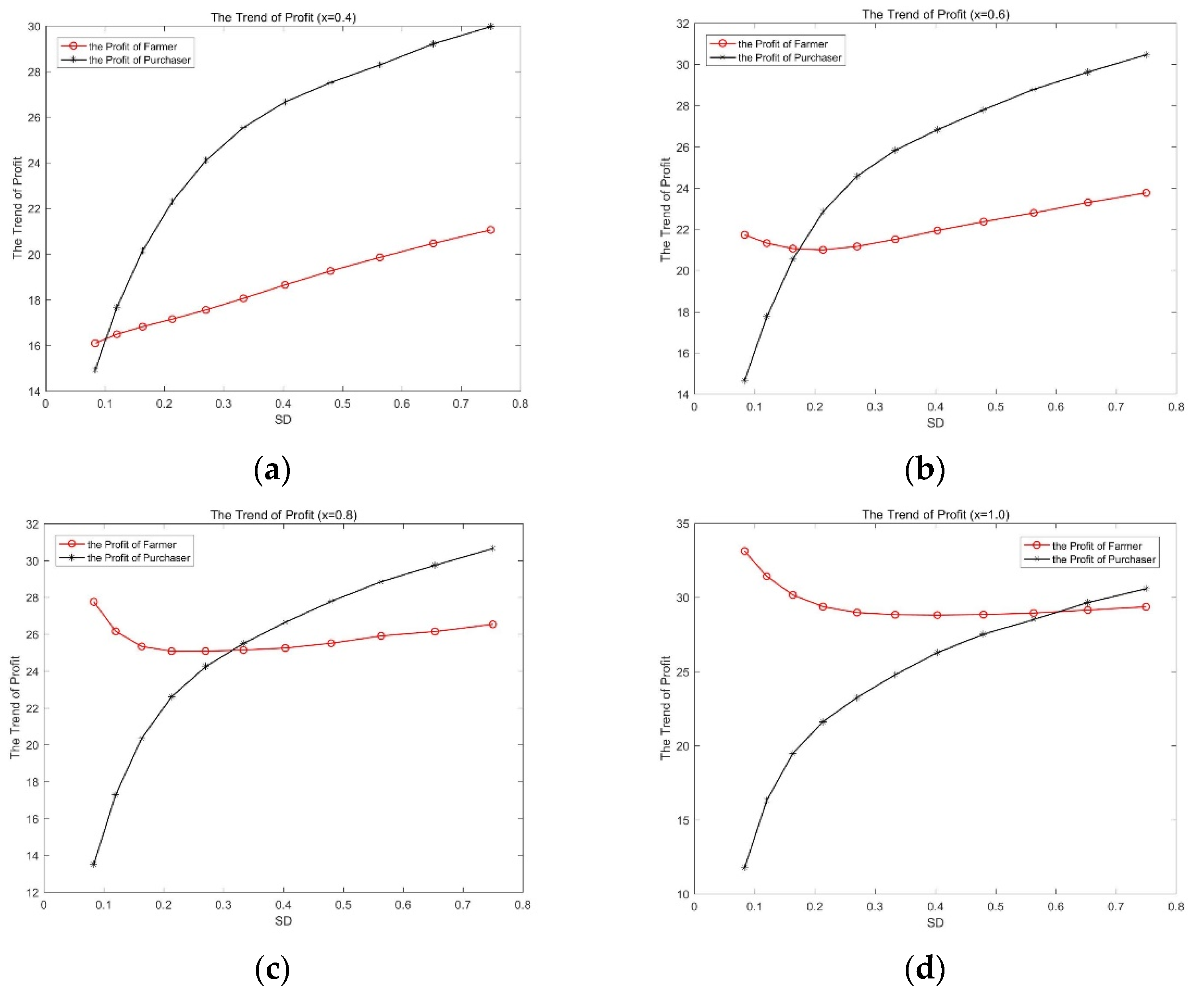
We suppose is between and . According to the characteristics of the uniform distribution function, we can get . The horizontal axis represents the variance of the variable with uncertain output. Each graph is drawn by sequentially increasing the value of at the right endpoint of the interval while holding fixed. Figure 10a–d, respectively, represent the change in the graph for the case where the output becomes more desirable as the value of at the left endpoint is gradually increased.
The vertical axis of Figure 10 represents the profit of the farmer and the purchaser. In areas with relatively small variance, the profit of the farmer will have a small downward trend. This is because when output is in a less-than-ideal area, although the farmer have gradually expanded production with the increase in expected output, the increase in loan amount has also increased the pressure on the farmer to repay. In turn, the expected profits of the farmer have fallen. On the whole, the profits of the farmer and the purchaser are in direct proportion to the variance of because of the continuous increase in expected output. In addition, the purchaser will have a slowing turning point in the process of profit increase. This is still due to the constraints of the loan ceiling, which prevents the increase of the loan volume of the farmer. After the turning point, the profits of the purchaser only come from the increase in price gap from the product market not the borrowing market. With the gradual increase of the left endpoint value , the farmer’s returns as a whole clearly flatten upwards while the profit growth of the purchaser is not significant. There is even a negative growth (Figure 10c,d). The reason is similar to the previous analysis. When the output situation improves completely and the harvest is still better even if the worst scenario happens, the market price of agricultural products decreases significantly. It is detrimental for the purchaser who has already mad profits through larger price gap while the farmer is less affected.
4. Discussion
4.1. Conclusions and Policy Recommendations
In previous studies of internal financing models in agricultural supply chains, because the acquirer acts as the core supply chain firm providing loans to farmer, most studies have tacitly assumed that the purchaser bears the full risk associated with production. No consideration is given to the fact that when the core company is simultaneously issuing loans and purchasing agricultural products, it can maximize its own profits by controlling two decision variables at the same time, nor does it take into account the risk-sharing mechanisms that can be achieved through the pledging of fixed assets by farmer. Therefore, we study a secondary order agricultural supply chain finance model that includes a farmer and a purchaser under output uncertainty. The farmer owns the fixed assets for production and can pledge them in the model. In the framework of the Stackelberg game, the acquirer provides loans to farmer who is facing financial constraints on his production. At this point, the acquirer can determine both the interest rate on the loan and the ratio of wholesale to market price, while the decision variable for the farmer is the amount of the loan.
After numerical simulations, we came to the following conclusions:
- The introduction of a fixed asset collateral model in the agricultural supply chain effectively reduces the risk borne by the purchaser while increasing the profitability of the farmer. This is because by using fixed assets as collateral for loans, farmers are actively assuming some of the risks associated with production uncertainty. Risks are thus shared among the supply chain participants, and profits are redistributed between them;
- We examined the various factors that affect profitability under this lending model. It was found that the selection of high-end agricultural products for cultivation significantly increases the profitability of all participants in the supply chain;
- We find that a steady increase in output does not improve the overall profitability of the supply chain, as market prices would fall significantly as a result. The acquirer at this point is likely to use its strong negotiating position to drive down the purchase price in order to secure its own profits. This will eventually lead to the phenomenon of “cheap corps hurt the agricultures”, which will affect the incentive of farmers to produce.
Based on these conclusions, we offer the following policy recommendations for real-life application:
- The agricultural supply chain contract model proposed in this paper can effectively improve the probability of loan success, thus contributing to the long-term development of the agricultural supply chain. Acquirers and government departments can promote their use as they see fit;
- Government departments need to guide farmers in their production decisions and encourage them to produce high-end agricultural products. Local governments can provide appropriate targeted financial subsidies for this purpose;
- When necessary, government departments can make reasonable use of national granaries and other means to buy agricultural products directly from farmers. The purpose of this is twofold. Firstly, it prevents malicious purchases by buyers in high yield years, thus protecting the interests of farmers and reducing irrational factors that are detrimental to the long-term development of the market. The second is that when production technology improves rapidly, the government is able to take the initiative to pace development and artificially make the variance in the supply of agricultural products larger, so that the supply of agricultural products spirals upwards in terms of quantity.
4.2. Shortcomings and Further Research
Based on the set of assumptions made in this paper to simplify the analysis, as well as more complex external factors that we have not yet taken into account. There are at least the following shortcomings in this paper, as well as possible directions for further research based on them.
- This paper does not take into account government subsidies and agricultural insurance, which are traditional ways of reducing risk. This paper provides a new contractual model for agricultural supply chains, so using this model as a framework and continuing to include these traditional methods in subsequent studies can lead to further optimization of the model. It will also be more useful as a guide to practical work;
- For simplicity of analysis, it is assumed that the market can be cleared and that there is no depreciation on the pledged fixed assets that could result in a loss on realization. Further liberalization of such assumptions, while having no impact on the basic conclusions we draw, could be more in line with the more complex economic environment we actually face, leading to more meaningful research conclusions;
- External financing models such as loans from banks and other financial institutions are not included in this paper for comparative analysis. However, in the course of this paper, we can find that obtaining more external financial support can bring more opportunities for growth in the supply chain as a whole. Therefore, further expansion of the scope of the cross-sectional comparison can seek out a more reasonable model;
- On the basis of the conclusions we have drawn from the model construction, it is also of great interest to carry out an empirical analysis using real-world data. This will allow the conclusions presented in this paper to be further supported on a practical level.
Author Contributions
Conceptualization, L.D.; methodology, S.W.; validation, L.D., S.W. and Y.W.; software, S.W.; formal analysis, S.W. and Y.W.; investigation, Y.L.; resources, L.D.; data curation, S.W.; writing—original draft preparation, L.D.; writing—review and editing, S.W. and Y.W.; visualization, L.D. and S.W.; supervision, L.D. and Y.L.; project administration, L.D.; funding acquisition, L.D. All authors have read and agreed to the published version of the manuscript.
Funding
The article is supported by The National Social Science Fund of China (No. 19BGL002).
Data Availability Statement
Not applicable.
Conflicts of Interest
The authors declare no conflict of interest.
Appendix A. Proof of Proposition 1
To solve the optimization problem (P1), we take the partial derivative of the formula with respect to , which leads to the first-order optimal solution corresponding to the loan amount . The steps are as follows:
Let the above formula be equal to 0, and it can be known from the integral median theorem,
Satisfy
easy to know
so, when
let , we can get the amount of the loan
Appendix B. The Proof of Proposition 2
To solve the optimization problem (P2), we obtain partial derivatives of Formula (4) with respect to and respectively. The specific solving steps are as follows:
Note
Let both partial derivatives be 0 at the same time, namely
So, we get the conclusion of Proposition 2.
References
- Babbar, S.; Prasad, S. International purchasing, inventory management and logistics research: An assessment and agenda. Int. J. Phys. Distr. Log. 1998, 28, 403–433. [Google Scholar] [CrossRef]
- Simon, C.; Pietro, R.; Mihalis, G. Supply chain management: An analytical framework for critical literature review. J. Purch. Supply Manag. 2000, 6, 67–83. [Google Scholar]
- Baron, B. Point estimation and risk preferences. J. Am. Stat. Assoc. 1973, 68, 944–950. [Google Scholar] [CrossRef]
- Pasternack, B. Optimal pricing and return policies for perishable commodities. Market. Sci. 1985, 4, 166–176. [Google Scholar] [CrossRef]
- Cachon, G.; Lariviere, M. Supply chain coordination with revenue-sharing contracts: Strengths and limitations. Manag. Sci. 2005, 51, 30–44. [Google Scholar] [CrossRef] [Green Version]
- Wang, Y.Y.; Yu, Z.Q.; Shen, L.; Fan, R.; Tang, R. Decisions and coordination in e-commerce supply chain under logistics outsourcing and altruistic preferences. Mathematics 2021, 9, 253. [Google Scholar] [CrossRef]
- David, B.; John, F.; Björn, S. Enablers and barriers in German online food retailing. Supply Chain Forum 2014, 15, 4–11. [Google Scholar]
- Godsell, J.; Birtwistle, A.; Hoek, R. Building the supply chain to enable business alignment: Lessons from British American Tobacco (BAT). Supply Chain Manag. 2010, 15, 10–15. [Google Scholar] [CrossRef]
- Miles, R.E.; Snow, C.C. Organization theory and supply chain management: An evolving research perspective. J. Oper. Manag. 2007, 25, 459–463. [Google Scholar] [CrossRef]
- Gomm, M.L. Supply chain finance: Applying finance theory to supply chain management to enhance finance in supply chains. Int. J. Logist. Res. App. 2010, 13, 133–142. [Google Scholar] [CrossRef]
- Alavi, S.; Jabbarzadeh, A. Supply chain network design using trade credit and bank credit: A robust optimization model with real world application. Comput. Ind. Eng. 2018, 125, 69–86. [Google Scholar] [CrossRef]
- Buzacott, J.; Zhang, R. Inventory management with asset-based financing. Manag. Sci. 2004, 50, 1274–1292. [Google Scholar] [CrossRef]
- Klapper, L. The role of factoring for financing small and medium enterprises. J. Bank. Financ. 2006, 30, 3111–3130. [Google Scholar] [CrossRef] [Green Version]
- ManMohan, S.; Christopher, S. Special issue of production and operations management: Socially responsible operations. Prod. Oper. Manag. 2012, 21, 795–796. [Google Scholar]
- Lamoureux, M. Supply chain finance prime. Supply Chain Financ. 2007, 4, 34–48. [Google Scholar]
- Xu, X.; Birge, J. Joint production and financing decisions: Modeling and analysis. Supply Chain Financ. 2005, 4, 34–48. [Google Scholar] [CrossRef] [Green Version]
- Timme, S.; Williams, C. The financial-SCM connection. Supply Chain Manag. Rev. 2000, 4, 33–40. [Google Scholar]
- Hoffmann, E. Supply chain finance—Some conceptual insights. Beiträge zu Beschaffung und Logistik 2005, 1, 213–214. [Google Scholar]
- Christopher, S.; Tang, S.; Yang, A.; Wu, J. Sourcing from suppliers with financial constraints and performance risk. Manuf. Serv. Oper. Manag. 2018, 20, 70–84. [Google Scholar]
- Martin, A. The Places They Go When Banks Say No. New York Times. 31 January 2010. Available online: http://www.nytimes.com/2010/01/31/business/smallbusiness/31order.html?dbk (accessed on 17 November 2021).
- Tice, C. Can a Purchase Order Loan Keep Your Business Growing. Entrepreneur. 17 June 2010. Available online: http://www.entrepreneur.com/article/207058 (accessed on 17 November 2021).
- Gustin, D. Purchase Order Finance, the Tough Nut to Crack. Trade Financing Matters. 28 April 2014. Available online: http://spendmatters.com/tfmatters/purchase-order-finance-the-tough-nut-to-crack/ (accessed on 17 November 2021).
- Petersen, M.; Rajan, R. Trade credit: Theories and evidence. Rev. Financ. Stud. 1997, 10, 661–691. [Google Scholar] [CrossRef]
- Lamoureux, J.; Evans, T. Supply Chain Finance: A New Means to Support the Competitiveness and Resilience of Global Value Chains; Social Science Electronic Publishing: Rochester, NY, USA, 2012. [Google Scholar] [CrossRef]
- Deng, L.; Yang, L.; Li, W. Impact of green credit financing and carbon emission limits on the supply chain based on POF. Sustainability 2021, 13, 5814. [Google Scholar] [CrossRef]
- Yan, N.; Liu, C.; Liu, Y. Effects of risk aversion and decision preference on equilibriums in supply chain finance incorporating bank credit with credit guarantee. Supply Chain Manag. Rev. 2017, 33, 602–625. [Google Scholar] [CrossRef]
- Song, H.; Lu, Q. What kind of small and medium-sized enterprises can benefit from supply chain finance?—Based on the network and capability perspective. Manag. World 2017, 6, 104–121. [Google Scholar]
- Fang, L.; Xu, S. Financing equilibrium in a green supply chain with capital constraint. Comput. Ind. Eng. 2020, 143, 106390. [Google Scholar] [CrossRef]
- Wilson, T.P.; Clarke, W.R. Food safety and traceability in the agricultural supply chain: Using the Internet to deliver traceability. Supply Chain Manag. 1998, 3, 127–133. [Google Scholar] [CrossRef]
- Regan, A. Designing and managing the supply chain: Concepts, strategies, and case studies. Transport. Sci. 2002, 36, 354. [Google Scholar] [CrossRef] [Green Version]
- Wang, Y.; Gerchak, Y. Periodic review production models with variable capacity, random yield, and uncertain demand. Manag. Sci. 1996, 42, 130–137. [Google Scholar] [CrossRef]
- Zant, W. Hedging price risks of farmers by commodity boards: A simulation applied to the Indian natural rubber market. World Dev. 2001, 29, 691–710. [Google Scholar] [CrossRef]
- Bogetoft, P.; Olesen, H. Ten rules of thumb in contract design: Lessons from Danish agriculture. Eur. Rev. Agric. Econ. 2002, 29, 185–204. [Google Scholar] [CrossRef]
- Allen, S.; Schuster, E. Controlling the risk for an agricultural harvest. Manuf. Serv. Oper. Manag. 2004, 6, 225–236. [Google Scholar] [CrossRef] [Green Version]
- He, Y.; Zhang, J. Random yield risk sharing in a two-level supply chain. Int. J. Prod. Econ. 2008, 112, 769–781. [Google Scholar] [CrossRef]
- Sachiko, M.; Nicholas, M.; Hu, D. Impact of contract farming on income: Linking small farmers, packers, and supermarkets in China. World Dev. 2009, 37, 1781–1790. [Google Scholar]
- Inderfurth, K.; Vogelgesang, S. Concepts for safety stock determination under stochastic demand and different types of random production yield. Eur. J. Oper. Res. 2013, 224, 293–301. [Google Scholar] [CrossRef]
- Chen, Y.; Tu, H.; Zeng, Y. Loan pricing and production regulation mechanism of agricultural supply chain finance. Syst. Eng.-Theory 2018, 38, 1706–1716. [Google Scholar]
- Nong, G.; Pang, S. Coordination of agricultural products supply chain with stochastic yield by price compensation. IERI Procedia 2013, 5, 118–125. [Google Scholar] [CrossRef] [Green Version]
- Toole, C.; Hennessy, T. Do decoupled payments affect investment financing constraints? Evidence from Irish agriculture. Food Policy 2015, 56, 67–75. [Google Scholar]
- Huang, J.; Lin, Q. Government subsidy mechanism in contract-farming supply chain financing under loan guarantee insurance and output uncertainty. Chin. J. Manag. Sci. 2019, 27, 53–65. [Google Scholar]
- Cai, X.; Chen, J.; Xiao, Y. Fresh-product supply chain management with logistics outsourcing. Omega 2013, 41, 752–765. [Google Scholar] [CrossRef]
- Van, B.M.; Steeman, M.; Reindorp, M. Supply chain finance schemes in the procurement of agricultural products. J. Purch. Supply Manag. 2019, 25, 172–184. [Google Scholar]
- Niu, B.Z.; Shen, Z.F.; Xie, F.F. The value of blockchain and agricultural supply chain parties’ participation confronting random bacteria pollution. J. Clean. Prod. 2021, 319, 128579. [Google Scholar] [CrossRef]
- Yadav, V.S.; Singh, A.R.; Raut, R.D.; Govindarajan, U.H. Blockchain technology adoption barriers in the Indian agricultural supply chain: An integrated approach. Resour. Conserv. Recycl. 2020, 161, 104877. [Google Scholar] [CrossRef]
- Sharma, R.; Shishodia, A.; Kamble, S.; Gunasekaran, A.; Belhadi, A. Agriculture supply chain risks and COVID-19: Mitigation strategies and implications for the practitioners. Int. J. Logist. Res. App. 2020, 1–27. [Google Scholar] [CrossRef]
- Kouvelis, P.; Zhao, W.H. Financing the newsvendor: Supplier vs. bank, and the structure of optimal trade credit contracts. Oper. Res. 2012, 60, 566–580. [Google Scholar] [CrossRef]
- Bai, S.; Xu, N.; Yan, Z. Research on decisions on inventory financing based on core enterprise’s buy-back guarantee. Chin. J. Manag. Sci. 2012, 20, 309–314. [Google Scholar]
- Lin, L.; Guo, X.; Hu, Z.; Liang, L. The risk-sharing contracts under random yield and stochastic demand in agricultural supply chain. Chin. J. Manag. Sci. 2013, 2, 50–57. [Google Scholar]
- Stackelberg, H.V. Market Structure and Equilibrium; Springer: Berlin/Heidelberg, Germany, 2011. [Google Scholar]
- Bernstein, F.; Federgruen, A. Decentralized supply chains with competing retailers under demand uncertainty. Manag. Sci. 2005, 51, 18–29. [Google Scholar] [CrossRef] [Green Version]
- Hang, L.T.; Tung, N.S. Supply chain finance for SMEs—Case in danang city. Oper. Supply Chain Manag. 2019, 12, 237–244. [Google Scholar] [CrossRef]
- Cai, X.; Chen, J.; Xiao, Y. Optimization and coordination of fresh product supply chains with freshness-keeping effort. Prod. Oper. Manag. 2010, 19, 261–278. [Google Scholar] [CrossRef]
- Lin, Q.; Ye, F. Nash negotiation model of “company + farmers”-based contract agricultural supply chain. Syst. Eng.-Theory 2014, 34, 1769–1778. [Google Scholar]
Figure 1.
The timeline of this loan.

Figure 2.
The profit trend of purchaser and farmer. (a) Trend of purchaser’s profits influenced by their own decision variables; (b) Trends in farmer profits influenced by their own decision variables.
Figure 2.
The profit trend of purchaser and farmer. (a) Trend of purchaser’s profits influenced by their own decision variables; (b) Trends in farmer profits influenced by their own decision variables.

Figure 3.
Trend of purchaser’s profit influenced by its own decision variables under different fixed asset values. (a) For fixed assets a = 8.0; (b) For fixed assets a = 10.0; (c) For fixed assets a = 12.0.
Figure 3.
Trend of purchaser’s profit influenced by its own decision variables under different fixed asset values. (a) For fixed assets a = 8.0; (b) For fixed assets a = 10.0; (c) For fixed assets a = 12.0.

Figure 4.
Trend of farmer’s profit influenced by its own decision variables under different fixed asset values.
Figure 4.
Trend of farmer’s profit influenced by its own decision variables under different fixed asset values.

Figure 5.
In the case of continuous changes in the value of fixed assets. (a) The trend of each decision variables; (b) The trend of the profit of the purchaser and the farmer.
Figure 5.
In the case of continuous changes in the value of fixed assets. (a) The trend of each decision variables; (b) The trend of the profit of the purchaser and the farmer.

Figure 6.
The trend of each decision variables under continuous changes in . (a) In the case of other parameters are taken as base values; (b) Expand the range of values of the loanable amount, such that .
Figure 6.
The trend of each decision variables under continuous changes in . (a) In the case of other parameters are taken as base values; (b) Expand the range of values of the loanable amount, such that .

Figure 7.
The trend of the profit of the purchaser and the farmer under continuous changes in . (a) In the case of other parameters are taken as base values; (b) Expand the range of values of the loanable amount, such that .
Figure 7.
The trend of the profit of the purchaser and the farmer under continuous changes in . (a) In the case of other parameters are taken as base values; (b) Expand the range of values of the loanable amount, such that .

Figure 8.
The trends of all decision variables in the presence of sustained improvements in output. (a) In the case of other parameters are taken as base values; (b) Expand the range of values of the ratio of the purchase price to the market price, such that .
Figure 8.
The trends of all decision variables in the presence of sustained improvements in output. (a) In the case of other parameters are taken as base values; (b) Expand the range of values of the ratio of the purchase price to the market price, such that .

Figure 9.
The trends of the profit of the purchaser and the farmer in the presence of sustained improvements in output. (a) In the case of other parameters are taken as base values; (b) Expand the range of values of the ratio of the purchase price to the market price, such that .
Figure 9.
The trends of the profit of the purchaser and the farmer in the presence of sustained improvements in output. (a) In the case of other parameters are taken as base values; (b) Expand the range of values of the ratio of the purchase price to the market price, such that .

Figure 10.
When the variance of output continues to increase, the trend of profit of the purchaser and the farmer. (a) In the case of the worst output x = 0.4; (b) x = 0.6; (c) x = 0.8; (d) x = 1.0.
Figure 10.
When the variance of output continues to increase, the trend of profit of the purchaser and the farmer. (a) In the case of the worst output x = 0.4; (b) x = 0.6; (c) x = 0.8; (d) x = 1.0.


Table 1.
List of notations.
| Notation | Description |
|---|---|
| The value of fixed assets used as collateral | |
| The loan volume | |
| The loan interest rate | |
| The ratio of the purchase price to the market price | |
| The uncertainty variable in farm household output | |
| The cumulative probability distribution of the output | |
| The probability density of the output | |
| The volume of agricultural products produced | |
| The market price of unit product | |
| The purchase price of unit product | |
| The inverse of the price elasticity of demand | |
| The farmer’s profit | |
| The purchaser’s profit |
Table 2.
Numerical algorithm results.
| Notation | Description | Numerical Value |
|---|---|---|
| The amount of loan | 90,000 | |
| The loan interest rate | 3% | |
| The ratio of acquisition price to market price | 0.5 | |
| The farmer’s profit | 27.84 | |
| The purchaser’s profit | 13,570,000 |
Publisher’s Note: MDPI stays neutral with regard to jurisdictional claims in published maps and institutional affiliations. |
© 2021 by the authors. Licensee MDPI, Basel, Switzerland. This article is an open access article distributed under the terms and conditions of the Creative Commons Attribution (CC BY) license (https://creativecommons.org/licenses/by/4.0/).
Share and Cite
MDPI and ACS Style
Deng, L.; Wang, S.; Wen, Y.; Li, Y. Incorporating ‘Mortgage-Loan’ Contracts into an Agricultural Supply Chain Model under Stochastic Output. Mathematics 2022, 10, 85. https://0-doi-org.brum.beds.ac.uk/10.3390/math10010085
AMA Style
Deng L, Wang S, Wen Y, Li Y. Incorporating ‘Mortgage-Loan’ Contracts into an Agricultural Supply Chain Model under Stochastic Output. Mathematics. 2022; 10(1):85. https://0-doi-org.brum.beds.ac.uk/10.3390/math10010085
Chicago/Turabian StyleDeng, Liurui, Shuge Wang, Yixuan Wen, and Yuting Li. 2022. "Incorporating ‘Mortgage-Loan’ Contracts into an Agricultural Supply Chain Model under Stochastic Output" Mathematics 10, no. 1: 85. https://0-doi-org.brum.beds.ac.uk/10.3390/math10010085
Note that from the first issue of 2016, this journal uses article numbers instead of page numbers. See further details here.