Software Release Assessment under Multiple Alternatives with Consideration of Debuggers’ Learning Rate and Imperfect Debugging Environment

Abstract

In the software development life cycle, the quality and reliability of software are critical to software developers. Poor quality and reliability not only cause the loss of customers and sales but also increase the operational risk due to unreliable codes. Therefore, software developers should try their best to reduce such potential software defects by undertaking a software testing project. However, to pursue perfect and faultless software is unrealistic since the budget, time, and testing resources are limited, and the software developers need to reach a compromise that balances software reliability and the testing cost. Using the model presented in this study, software developers can devise multiple alternatives for a software testing project, and each alternative has its distinct allocation of human resources. The best alternative can therefore be selected. Furthermore, the allocation incorporates debuggers’ learning and negligent factors, both of which influence the efficiency of software testing in practice. Accordingly, the study considers both human factors and the nature of errors during the debugging process to develop a software reliability growth model to estimate the related costs and the reliability indicator. Additionally, the issue of error classification is also extended by considering the impacts of errors on the system, and the expected time required to remove simple or complex errors can be estimated based on different truncated exponential distributions. Finally, numerical examples are presented and sensitivity analyses are performed to provide managerial insights and useful directions to inform software release strategies.

1. Introduction

Nowadays, software reliability is always an important indicator for evaluating software quality and can be used as a basis to make an appropriate plan for software testing work. In modern software industries, software developers not only focus on the functionality of their developed software or systems but also ensure that software quality and stability are over an acceptable level. Once the software quality and stability cannot satisfy their clients’ or customers’ requirements, this will still cause the loss of sales or customer dissatisfaction no matter how superior the functionality and performance of software/system might be. However, due to the constraints of the project budget, human resources, and testing time, it is unrealistic for software developers to pursue a perfect and faultless software/system. Accordingly, in practice, most software developers will make a compromise plan instead of spending a huge budget pursuing a faultless software/system. Over the past few decades, various software reliability growth models (SRGMs) have been proposed, and most of them adopt a Non-Homogeneous Poisson Process (NHPP) to describe software testing and debugging phenomena [1,2,3,4,5,6,7,8,9,10,11,12,13,14,15,16,17,18,19,20,21].

Generally, testing staff’s learning and experience will influence the debugging efficiency, and the velocity of error detection will increase in the mid to late testing phase. Therefore, the curve of the mean value function of a software reliability growth model (SRGM) will present an S-shaped form. Yamada et al. [2] proposed an S-shaped reliability growth model for software error detection but they did not clearly point out which parameters are related to the learning factor in their proposed model. Li and Pham [22] took failure intensity functions into consideration for presenting a learning effect during a testing process. Huang et al. [23] developed an SRGM which considered testing effort. They believed that the efficiency of error detection may be lower in the early stage but that the growth rate of error detection will accelerate in the mid-stage. Therefore, the curve of the SRGM will present as S-shaped, indicating the learning effect that occurs in debugging works. Chiu et al. [7] state that the learning effect should be considered a crucial parameter in SRGM, and the value of this parameter can be used to estimate the inflection point during a testing period. In their experiments, the curve of SRGM can adapt to concave or S-shape forms, reflecting the learning effect that exists in testing works. Moreover, due to the fact that the parameter of the learning effect might be hard to estimate if the related historical data are insufficient, the decision-maker needs to utilize other methods for evaluating the parameters’ value. In order to solve this issue, Chiu et al. [24] extended their original model by utilizing a Bayesian method to reasonably estimate the parameters’ value regarding the learning effect. However, their research concerns perfect debugging SRGMs, and they did not take the testing staff’s negligence into consideration. Besides, they simply assumed that all software errors would be homogeneous, an unrealistic assumption because different error types will require different amounts of time to be rectified. Ahmad et al. [25] proposed a testing-effort dependent inflection S-Shaped SRGM that includes the learning effect in the software testing process. Raju [26] also proposed an inflection S-shaped software reliability model based on NHPP, and their model can be adapted to exponential and S-shaped data. Ramsamy et al. [27] state that most SRGMs do not take the learning factors of testing staff into consideration. In order to improve the adaptability of various software testing projects, they utilized learning and debugging indices to develop an SRGM. Kim and Kim [28] proposed SRGMs that were sensitive to learning effects by using Yamada and Ohba’s delayed S-shaped models. The study discussed the relationship between release time and testing efforts to minimize software development. Pachauri et al. [29] took the S-shaped curve, imperfect debugging, and error reduction factors into consideration to develop a multi-stage SRGM. Jin and Jin [30] extended the study of Huang et al. [23] to propose an SRGM that included testing effort, and their model can accommodate exponential and S-shaped data patterns simultaneously. Chiu et al. [31] extended their former model and assumed that the learning effect can be time-dependent and may grow linearly or exponentially with testing time. In addition, their extended model can describe the phenomenon of unstable debugging efficiency during the early testing stage. Based on the above discussion, it can be noted that although the learning effect has been taken into consideration in previous research, this work has not fully considered all possible factors regarding human resource issues, including the basic ability, learning efficacy, and negligent factor of testing staff. Accordingly, the present study will incorporate all of these elements to propose a software release decision model SRGM under multiple alternatives.

Moreover, most of the related studies only considered the scenario of perfect debugging. They simply assumed that the testing/debugging staff would not make mistakes again when they corrected the error codes. However, such an assumption might be unrealistic because humans are not perfect in nature, and it cannot be ruled out that testing/debugging staff’s carelessness may introduce new software defects. Therefore, recently, some studies have begun to investigate the issue of imperfect debugging SRGMs. Aktekin and Caglar [32] proposed a multiplicative failure rate that varied randomly during the test phase, and the model could explain the phenomenon of imperfect debugging in practice. Peng et al. [33] proposed an SRGM that considered testing-effort allocation for imperfect debugging processes. They designed three testing-effort functions (constant, Weibull, and logistic forms) to describe how the software developer allocates testing resources during a time horizon. Wang and Wu [34] proposed an imperfect debugging SRGM by utilizing a fault content function with a log-logistic distribution. They assumed that testing/debugging staff’s skills, case tools, and testing resources are complex and uncertain factors that significantly influence the testing process. Therefore, these factors might cause new software faults, which were produced in the testing process. Zhu and Pham [35] proposed a multi-release software reliability model that considered the remaining software faults from previous software releases and newly introduced faults different from those that existed earlier. Li and Pham [36] also highlighted that debugging and test coverage might not be perfect, since the operating environment might be uncertain and varied for testing projects. Therefore, they proposed a model that used randomly distributed variables to simulate the uncertainty of the operating environment. Zhao et al. [37] took the factors of perfect and imperfect debugging into consideration to propose a Bayesian SRGM to deal with the issue of the uncertainty of software reliability. Saraf and Iqbal [38] developed an SRGM that incorporated two types of imperfect debugging and the change-point factor to deal with the issue of multiple versions for a software release. Li et al. [39] proposed an NHPP-based SRGM that concerns testability growth effort, rectifying delays, and imperfect debugging. Within the above-mentioned studies, the common assumption is that new software errors are simply introduced with testing time. However, pure testing work is only used to discover errors in the system and should not produce any new errors because program codes are not changed during pure testing work. Therefore, in this study, the software error correction process and debugging staff’s negligence are considered, and our assessment of efficiency includes the results from the detected software error patterns. This is different from the idea of a traditional imperfect debugging SRGM.

It is easy to understand how the processing time for removing or correcting each error could be different, because different types of errors need different amounts of time to be corrected. Furthermore, the processing time for removing or correcting an error should be regarded as a random variable, which needs to be estimated in advance from the related historical data. However, most existing SRGMs simply assume that such processing time is constant and unitary. Obviously, this assumption might be unrealistic in practice. Accordingly, some related studies have begun to revise the former assumption and focus on the issue of multiple error types in order to improve the practicality of SRGMs. Kapur et al. [9,10] assumed that error detection rates are different for various error types. In their model, the errors can be classified as simple, difficult, and complex types. Jain et al. [40] constructed an SRGM that considered simple and complex errors during the debugging process. Garmabaki et al. [41] examined software version up-gradation and error conditions with different degrees of severity to construct software reliability models for different software versions, in which the number of error removals in each version included the detected errors in the current version and those left from the previous versions. Khatri and Chhillar [42] classified software faults into three types (simple, difficult, and complex) to develop an imperfect SRGM. This classification was conducted according to the degree of error correction difficulty. Kaushal and Khullar [43] proposed Neural Network Approaches to predict software errors for NASA’s public defect datasets. They classified software faults into different types according to the severity of the damage caused by the fault. Song and Rhew [44] developed a method for identifying the types of software errors automatically. They roughly classified software errors into logic, data, interface, document, and computational problems. Wang et al. [45] also took two types of faults into consideration to propose an SRGM and assumed that the two types of faults are mutually independent. Zhu and Pham [46] proposed a two-phase SRGM that considered software error dependency and imperfect fault removal, and they assumed the occurrence of two types of software error during the two-phase debugging process. Huang et al. [47] also considered two types of software error to develop an imperfect debugging SRGM. Based on the above discussion, previous studies have taken the issue of multiple error types into consideration because the correction for a complex error usually requires more time than a simple one does, and it is inappropriate to calculate the estimated time and cost for different error types by using a unified setting. Moreover, different errors require different processing time during a correction, and therefore the processing time for removing or correcting an error should be regarded as a random variable instead of a constant value. The decision-maker can reasonably estimate it by using the related operational data. However, most of the related studies have failed to recognize this factor. Accordingly, in order to increase practicability, our study assumes that the processing time for removing or correcting different error types follows specified probability distributions with different parameters.

In general, the testing environment might be changed due to increasing testing staff, upgrades to hardware, or changing case tools, and these factors will cause changes in debugging efficiency. The timing of changes in the testing environment is known as a change-point within the SRGM. Huang [5] proposed an SRGM that considered both testing effort and change-points. Huang and Hung [48] extended their former model to propose a model with multiple change-points based on the assumption that software developers will upgrade the developed software many times during a software’s life cycle in practice. Hu et al. [49] proposed a modified adaptive testing model, and considered how a testing environment may be changed due to the change in a testing policy. Inoue et al. [50] proposed an all-stage truncated multiple change-point model for assessing software reliability. They utilized a zero-truncated Poisson distribution to describe the counting process for software errors. Nagaraju et al. [51] proposed an SRGM that incorporated heterogeneous change-points and an error detection process that can be characterized by different time segments. Ke and Huang [52] highlighted that a development environment or method might be changed for some reason, and that such changes in the development process must be taken into consideration when adjusting the former analysis regarding software reliability. Pradhan et al. [53] also took the change-point issue into consideration when they proposed a testing-effort-based NHPP software reliability growth model. Khurshid et al. [54] proposed an imperfect debugging model, and they integrated testing effort, the fault-reduction factor, and change-point issues into their study. SRGMs that incorporate the change-point issue can bring more flexibility than the traditional models when the software developers face varied development or running environments. Accordingly, in this study, the change-point issue is taken into consideration, since, in practice, a software developer may increase manpower and resources within a testing system to accelerate testing tasks, and these changes might result in a change in software reliability. Thus, the current study incorporates these practical considerations within its model.

To sum up, this study considers the multiple issues of software testing in order to construct a software reliability growth model under multiple alternatives. Furthermore, the best timing for software release can be evaluated by considering reliability and cost. In addition, the parameters of the proposed model are more intuitive and can be more easily estimated or evaluated. Accordingly, we consider our study to be helpful to software industries aiming to release their software products or systems to the market. We identify three advantages of the present study, as follows: (1) The study integrates the issues of learning effect, human factors, imperfect debugging, multiple errors classification, change-point, etc., to construct a software reliability growth model under multiple alternatives. It is different from most of the related studies, which only take some of these factors into consideration. (2) The proposed model exhibits better performance with regards to goodness-of-fit compared with other existing models in statistical analyses. The estimation methods of the parameters’ values and confidence intervals are also developed in this study. (3) The model presented in this study is easier for practical applications. The optimal timing for software release can be obtained by the proposed model in terms of testing cost under the constraint of software reliability. The managers can evaluate all the feasible alternatives and decide on one of them before proceeding with software testing work. The rest of this paper is organized as follows: Section 2 presents the development of the model, parameter estimation, and the optimal software release model. Section 3 provides the model verification and comparison. The application and numerical analysis are presented in Section 4. Finally, Section 5 draws the concluding remarks and identifies topics for future studies.

2. Software Reliability Modeling

In recent years, NHPP has been widely and successfully used to examine reliability issues for a range of hardware and software applications. NHPP is a derivative of HPP; the major difference between these two stochastic processes is that the NHPP allows for the expected number of failures to vary with time. Since expected software faults decrease with testing time during the debugging process, it is suitable for application within software reliability growth models.

An implemented software system needs to be tested and debugged in advance to ensure quality when the system is released to the market. Several feasible alternatives can be designed and prepared for the software department or company, with the decision-maker selecting the best option for the software testing work. To balance system stability and related costs, the managers need to know the efficiency of any system reliability improvements under different resource allocations. Therefore, the managers will estimate the testing/debugging efficiency and the spending budget under several resource alternatives in advance. However, it is not easy to effectively estimate testing/debugging efficiency when the managers want to design and change input resources over time. Moreover, the environment of software testing might be changed or adjusted in practice due to changing testing staff, hardware, tools, or strategies midway through the testing process, and these changes may result in changes in testing/debugging efficiency. Accordingly, it is necessary to develop an effective SRGM that can deal with such issues of multiple testing alternatives or testing environment changes.

Generally, the process of software reliability growth can be described by mathematical functions as a counting process, $\left\{N\left(t\right), t\ge 0\right\}$, where $N\left(t\right)$ follows an NHPP with the mean value function $M\left(t\right)$, and this probability can be formulated as follows:

$$\mathrm{Pr}\left(N\left(t\right)=k\right)=\frac{{\left[M\left(t\right)\right]}^k{e}^{-M\left(t\right)}}{k!}, k=0,1,2,\dots$$

(1)

From another perspective, the mean value function can be expressed as the expected number of errors detected within the time period $\left[0,t\right]$:

$$M\left(t\right)={{\displaystyle \int }}_0^t\lambda \left(x\right)dx.$$

(2)

Furthermore, software reliability $R(x | t)$ can be defined as the probability of no errors being detected within the time period $\left[t,t+x\right]$, and it can be formulated as follows:

$$R(x | t)=e^{-\left[M\left(t+x\right)-M\left(t\right)\right]}.$$

(3)

The operating time $x$ is for the requirements of stability in practice, and the decision-maker can give an adequate value for managerial requirements. Note that enlarging the operating time will decrease the value of reliability. In addition, the value of software reliability will finally approach one when testing time approaches infinity ($\underset{t\to \infty }{\lim }R(x | t)\to 1$). The notations and terminologies are presented in

Table 1. The Notations and Terminologies.

$f\left(t\right)$: the intensity function of the fraction of the errors detected at time $t$

$F\left(t\right)$: the cumulative fraction of the errors detected in the time interval (0,$t$)

$\alpha$: the autonomous errors-detected factor

$\beta$: the learning factor

$\gamma$: the negligent factor

$a$: the initial number of all potential errors in the software system

$A\left(t\right)$: the function of the total errors at time $t$ in the software system

$M\left(t\right)$: the mean value function, and it represents the accumulated number of software errors detected during the time interval (0,$t$)

$M_v^p\left(t\right)$: the mean value function for alternative $p$ with testing environment $v$ ($v=b$, before changing point $\tau$; $v=f$, after changing point $\tau$)

$M_v^{p,y}\left(t\right)$: the mean value function for alternative $p$ with testing environment $v$ for error type $y$

$\lambda \left(t\right)$: the intensity function that denotes the number of the errors detected at time $t$

$D\left(t\right)$: the function of the error detection rate

$R\left(x|t\right)$: the software reliability, which is defined as the probability of no errors being detected within the time interval $\left[t,t+x\right]$

$G_y\left({\theta }_y,{\xi }_y\right)$: the probability density function of the time for correcting an error type y=s (simple errors), y = d (difficult errors) or y = c (complex errors));

$t_r$: The time required for performing a correction of software error

${\xi }_y$: The pre-specified upper time limit for performing a correction of software error type $y$

${\theta }_y$: the parameter of the function $G_y\left({\theta }_y,{\xi }_y\right)$; ${\widehat{\theta }}_y$ denote the estimator of ${\theta }_y$

$E\left[{\theta }_y,{\xi }_y,t_r\right]$: the expected time for performing a correction of software error type $y$ under parameters ${\xi }_y$ and ${\theta }_y$

$R_{mr}$: the minimal requirement of the system’s reliability for testing alternatives

, and they will be used throughout the study:

2.1. Basic Model Development

In general, it is unrealistic to assume that testing work will be conducted under perfect debugging conditions because the debugging staff may always produce new errors or bugs when removing and correcting the detected ones. Therefore, some of the related studies have made the assumption that software errors may be increased by testing time, and this can be called the issue of imperfect debugging in SRGM. In our proposed model, the major influential factors include testing staffs’ autonomous errors-detected factor $\alpha$, learning factor $\beta$, and negligent factor $\gamma$. 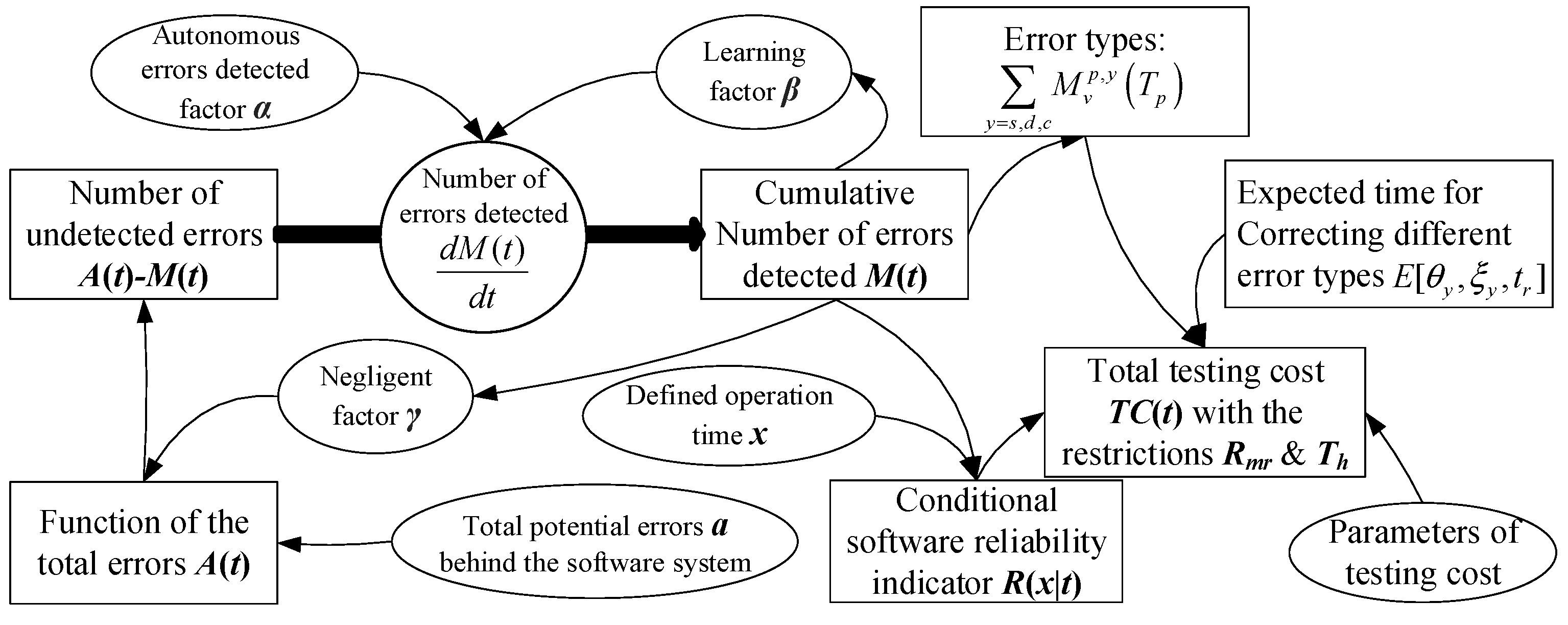It should be noted that the values of the parameters $\alpha$, $\beta$, and $\gamma$ must be greater than zero. In order to describe the concept of the proposed model, a causal loop diagram is used to illustrate the process of software reliability growth. Figure 1 illustrates the logical concept of the process of the software testing/debugging task, and the total efficiency of error detection is associated with the three factors. The arrows indicate the direction of influence among these factors and/or components. The circles represent the factors regarding debugging works and testing costs. The rectangles represent the relevant components. Additionally, the meaning of the mean value function $M\left(t\right)$ can be regarded as the average of the cumulative number of errors detected. Therefore, the function $M\left(t\right)$ is used to estimate the expected cumulative number in practice. However, if we take the stochastic issue into consideration, the actual cumulative number will be influenced by random noise. Such a definition was often seen in similar studies.

In this causal loop diagram, the autonomous errors-detected factor $\alpha$ can be described as the rate at which testing staff can find errors by their original ability. In other words, these are software errors spontaneously found by testing staff without any reference to the previous error patterns. Therefore, this ability originates from the testing staff’s intelligence and previous training, and it is unrelated to the learning factor, i.e., knowledge acquired from the current project. Furthermore, the learning factor $\beta$ indicates the testing staff’s learning ability, which is based on the previous error patterns. Therefore, the learning effect would increase with the testing time. Both factors can improve the efficiency of software debugging. However, the negligent factor $\gamma$ is the main cause of the phenomenon of imperfect debugging, and it can be regarded as the increased rate of new errors due to the debugging staff’s carelessness. In other words, the negligent factor negatively impacts on the efficiency of debugging, and it will increase the number of software errors. In this study, the number of the total software errors is set as a function of testing time, and we consider its increment to be related to the mean value function $M\left(t\right)$. Therefore, the function of the total software errors can be defined as follows:

$$A\left(t\right)=a+\gamma M\left(t\right),$$

(4)

where $a$ is the initial number of potential errors before the testing work started, and the new errors are those introduced along with the revised codes. The negligent factor $\gamma$ can be regarded as the rate of increase and is related to the accumulated number of software errors detected. In addition, $F\left(t\right)$ represents the cumulative fraction of the errors detected within the time range (0,$t$), and $A\left(t\right)-M\left(t\right)$ signifies the undetected errors at time $t$. Accordingly, the process of the detection can be described using the following differential equation:

$$D\left(t\right)=\frac{dM\left(t\right)}{A\left(t\right)-M\left(t\right)}=\alpha +\beta F\left(t\right)$$

(5)

where the parameters $\alpha$ and $\beta$ must be greater than or equal to zero to ensure the effect of debugging activity is positive in the testing process. Equations (4) and (5) imply that the learning effect and imperfect debugging exist in the testing process. Accordingly, the mean value function $M\left(t\right)$ can be derived by using differential equation methods; the following steps are the process for deducing the function $M\left(t\right)$.

Since the cumulative fraction of the original detected pattern $F\left(t\right)$ is defined as $M\left(t\right)/a$ and the total errors increase with testing time, i.e., $A\left(t\right)=a+\gamma M\left(t\right)$, Equation (5) can be rewritten as $D\left(t\right)=\frac{dM\left(t\right)}{a-\left(1-\gamma \right)M\left(t\right)}=\alpha +\left(\frac{\beta }{a}\right)M\left(t\right)$. In order to deduce the math form of $M\left(t\right)$, we arrange the equation in the following steps:

$$dM\left(t\right)=\left(a-\left(1-\gamma \right)M\left(t\right)\right)\left(\alpha +\left(\frac{\beta }{a}\right)M\left(t\right)\right)$$

(6)

$$\Rightarrow \frac{dM\left(t\right)}{\left(a-\left(1-\gamma \right)M\left(t\right)\right)\left(\alpha +\left(\frac{\beta }{a}\right)M\left(t\right)\right)}=1$$

Taking the integral of both sides of the equation, we can obtain the result as follows:

$$\int \frac{dM\left(t\right)}{\left(a-\left(1-\gamma \right)M\left(t\right)\right)\left(\alpha +\left(\frac{\beta }{a}\right)M\left(t\right)\right)}dt=\int 1dt$$

$$\frac{\ln \left(a-\left(1-\gamma \right)M\left(t\right)\right)-\ln \left(a\alpha +\beta M\left(t\right)\right)}{-\beta -\alpha \left(1-\gamma \right)}=t+const$$

(7)

Solving the above equation for $M\left(t\right)$, we can obtain the math form of $M\left(t\right)$ with the unknown constant as the following equation:

$$M\left(t\right)=\frac{-a{e}^{\left(\alpha +\beta \right)\left(t+const\right)}+a\alpha e^{\alpha \gamma \left(t+const\right)}}{-\beta e^{\alpha \gamma \left(t+const\right)}+\left(\gamma -1\right)e^{\left(\alpha +\beta \right)\left(t+const\right)}}$$

(8)

Since the initial condition $M\left(0\right)=0$ is given (no error detected at testing time $t=0$), we can use it to solve the value of the unknown constant as follows:

$$M\left(0\right)=\frac{a{e}^{\left(\alpha +\beta \right)const}-a\alpha e^{\left(\alpha \gamma \right)const}}{\beta e^{\left(\alpha \gamma \right)const}+\left(1-\gamma \right)e^{\left(\alpha +\beta \right)const}}=0$$

(9)

Solving Equation (8) for the unknown constant, the constant can be obtained as follows:

$$const=\frac{\ln \left(\alpha \right)}{\left(1-\gamma \right)\alpha +\beta }$$

(10)

Substituting the constant into Equation (8), we can obtain the complete form of $M\left(t\right)$ as follows:

$$M\left(t\right)=\frac{a{e}^{\left(\alpha +\beta \right)\left(t+\ln \alpha )/\left(\left(1-\gamma \right)\alpha +\beta \right)\right)}-a\alpha e^{\alpha \gamma \left(t+\ln \left(\alpha \right)/\left(\left(1-\gamma \right)\alpha +\beta \right)\right)}}{\beta e^{\alpha \gamma \left(t+\ln \left(\alpha \right)/\left(\left(1-\gamma \right)\alpha +\beta \right)\right)}+\left(1-\gamma \right)e^{\left(\alpha +\beta \right)\left(t+\ln \left(\alpha \right)/\left(\left(1-\gamma \right)\alpha +\beta \right)\right)}}$$

(11)

Since $e^{\ln \left(\alpha \right)}=\alpha$, the form of $M\left(t\right)$ can be simplified as follows:

$$M\left(t\right)=\frac{a{\alpha }^{\frac{\alpha +\beta }{\left(1-\gamma \right)\alpha +\beta }}\left(e^{\alpha \gamma t}-e^{\left(\alpha +\beta \right)t}\right)}{\beta {\alpha }^{\frac{\alpha \gamma }{\left(1-\gamma \right)\alpha +\beta }}{e}^{\alpha \gamma t}+\left(1-\gamma \right){\alpha }^{\frac{\alpha +\beta }{\left(1-\gamma \right)\alpha +\beta }}{e}^{\left(\alpha +\beta \right)t}}$$

(12)

Furthermore, the intensity function $\lambda \left(t\right)$, i.e., the number of the errors detected at time $t$, can be obtained as follows:

$$\lambda \left(t\right)=\frac{dM\left(t\right)}{dt}=\frac{a{\alpha }^{\frac{\alpha +\beta }{\left(1-\gamma \right)\alpha +\beta }}\left(\left(1-\gamma \right)\alpha +\beta \right)\left(\left(1-\gamma \right){\alpha }^{\frac{\alpha +\beta }{\left(1-\gamma \right)\alpha +\beta }}+\beta {\alpha }^{\frac{\alpha \gamma }{\left(1-\gamma \right)\alpha +\beta }}\right)e^{\left(\left(1+\alpha \right)\gamma +\beta \right)t}}{{\left(\left(1-\gamma \right){\alpha }^{\frac{\alpha +\beta }{\left(1-\gamma \right)\alpha +\beta }}{e}^{\left(\alpha +\beta \right)t}+\beta {\alpha }^{\frac{\alpha \gamma }{\left(1-\gamma \right)\alpha +\beta }}{e}^{\alpha \gamma t}\right)}^2}.$$

(13)

In order to handle the variation of the error detection rate per error at time $t$, the form of the error detection rate needs to be known and can be derived by Equations (4), (6), and (12), as follows:

$$D\left(t\right)=\frac{dM\left(t\right)}{A\left(t\right)-M\left(t\right)}=\frac{\left(\left(1-\gamma \right)\alpha +\beta \right){\alpha }^{\frac{\alpha +\beta }{\left(1-\gamma \right)\alpha +\beta }}}{\left(1-\gamma \right){\alpha }^{\frac{\alpha +\beta }{\left(1-\gamma \right)\alpha +\beta }}+\beta {\alpha }^{\frac{\alpha \gamma }{\left(1-\gamma \right)\alpha +\beta }}{e}^{\left(\alpha \gamma -\left(\alpha +\beta \right)\right)t}}.$$

(14)

The error detection rate is a strictly increasing function, which means that the testing staff’s efficiency is always improving in the process. Proposition A1 provides proof that the error detection rate is increasing at any testing time. Please see the proof in Appendix A.

In general, testing staff’s learning effect will present an acceleration phenomenon in the testing process. Once the acceleration phenomenon is significant, the mean value function will present as S-shaped. However, the means by which to verify the S-shaped mean value function depends on whether the inflection point is greater than zero or not. By referring to Proposition A2, we can see that the mean value function will show the acceleration phenomenon as S-shaped if the condition $\gamma >\frac{\alpha -\beta }{\alpha }$ is supported. The existence of an inflection point implies that the learning effect is significant in the testing process, and the inflection time point can be given by the following:

$$t_{\mathrm{inflection}}\approx \frac{\alpha \gamma \ln \left[\alpha \right]-\left(\left(1-\gamma \right)\alpha +\beta \right)\left(\ln \left[\frac{1-\gamma }{\beta }\right]{\alpha }^{\frac{\alpha +\beta }{\left(1-\gamma \right)\alpha +\beta }}\right)}{{\left(\left(1-\gamma \right)\alpha +\beta \right)}^2}.$$

(15)

The related proof of Proposition A2 can be seen in Appendix A.

2.2. Parameter Estimation

The two estimation methods can be applied to estimate the model parameters in this study. These collected software failure data are used to demonstrate the fitting degrees among the proposed model and other existing ones.

(1) The least-square estimation method (LSE) is a standard approach in statistics for estimating model parameters by minimizing the sum of the squares of the residuals. A set of $n$ pairs of observed data is taken into consideration, i.e., $\left(t_0,M_0\right),\left(t_1,M_1\right),\left(t_2,M_2\right),\dots ,\left(t_n,M_n\right)$, to estimate all parameters of the proposed model. Here, $M_i$ is the number of total detected errors within the period [$0,t_n]$, and the calculation can be given by the following:

$$Min Error\left(a,\alpha ,\beta ,\gamma \right)={{\displaystyle \sum }}_{i=1}^n{\left(M_i-M\left(t_i\right)\right)}^2 .$$

(16)

Taking the first-order derivative of Equation (16) with respect to each parameter and letting them be equal to zero, the simultaneous equations can be given as follows:

$$\frac{\partial Error\left(a,\alpha ,\beta ,\gamma \right)}{\partial a}=\frac{\partial Error\left(a,\alpha ,\beta ,\gamma \right)}{\partial \alpha }=\frac{\partial Error\left(a,\alpha ,\beta ,\gamma \right)}{\partial \beta }=\frac{\partial Error\left(a,\alpha ,\beta ,\gamma \right)}{\partial \gamma }=0.$$

(17)

Since the closed-form expression of the solution cannot be obtained, numerical methods are employed to solve the simultaneous equations to obtain the estimated parameter values. However, if software testing managers use an error seeding method to estimate parameter $a$ according to the system scale, the estimation of the remaining parameters will be simplified by solving the simultaneous equations $\frac{\partial Error(\alpha ,\beta ,\gamma |\widehat{a})}{\partial \alpha }=\frac{\partial Error(\alpha ,\beta ,\gamma |\widehat{a})}{\partial \beta }=\frac{\partial Error(\alpha ,\beta ,\gamma |\widehat{a})}{\partial \gamma }=0$.

(2) The maximum likelihood estimation method (MLE) is another approach to estimate the parameters of an assumed probability distribution. Due to the operation of a Non-Homogeneous Poisson Process, the likelihood function can be given as follows:

$$\begin{array}{ll}L\left[a,\alpha ,\beta ,\gamma \right]=& \mathrm{Pr}\left\{N\left(t_1\right)=M_1,N\left(t_2\right)=M_2,N\left(t_3\right)=M_3,\dots ,N\left(t_n\right)=M_n\right\}\\ & ={\displaystyle \prod }_{i=1}^n\frac{{\left(M\left(t_i\right)-M\left(t_{i-1}\right)\right)}^{\left(M_i-M_{i-1}\right)}\left(e^{-\left(M\left(t_i\right)-M\left(t_{i-1}\right)\right)}\right)}{\left(M_i-M_{i-1}\right)!}.\end{array}$$

(18)

Taking the natural logarithm of Equation (18), the likelihood function can be given as follows:

$$\begin{array}{ll}\ln \left[L\left[a,\alpha ,\beta ,\gamma \right]\right]=& {{\displaystyle \sum }}_{i=1}^n\left(M_i-M_{i-1}\right)\ln \left[M\left(t_i\right)-M\left(t_{i-1}\right)\right]-{{\displaystyle \sum }}_{i=1}^n(M\left(t_i\right)-\\ & M\left(t_{i-1}\right))-{\displaystyle \sum }_{i=1}^n\ln \left[\left(M_i-M_{i-1}\right)!\right].\end{array}$$

(19)

Likewise, taking the first-order derivative of Equation (19) with respect to each parameter and letting them be equal to zero, the simultaneous equations can be given as follows:

$$\frac{\partial \ln \left[L\left[a,\alpha ,\beta ,\gamma \right]\right]}{\partial a}=\frac{\partial \ln \left[L\left[a,\alpha ,\beta ,\gamma \right]\right]}{\partial \alpha }=\frac{\partial \ln \left[L\left[a,\alpha ,\beta ,\gamma \right]\right]}{\partial \beta }=\frac{\partial \ln \left[L\left[a,\alpha ,\beta ,\gamma \right]\right]}{\partial \gamma }=0.$$

(20)

The estimated values of these parameters can be obtained by solving the log-likelihood function with numerical methods. However, if an error seeding method can be employed to estimate the initial number of all potential errors in advance, the estimation of the remaining parameters will be simplified by solving the simultaneous equations as $\frac{\partial \ln \left[L\left[\alpha ,\beta ,\gamma |\widehat{a}\right]\right]}{\partial \alpha }=\frac{\partial \ln \left[L\left[\alpha ,\beta ,\gamma |\widehat{a}\right]\right]}{\partial \beta }=\frac{\partial \ln \left[L\left[\alpha ,\beta ,\gamma |\widehat{a}\right]\right]}{\partial \gamma }=0$.

In addition, the confidence interval for the parameters $\alpha ,\beta ,\mathrm{and} \gamma$ can be derived from the variance–covariance matrix $\sum$ for all the maximum likelihood estimators. The Fisher information matrix F can be used to obtain the variance–covariance matrix $\sum$ as follows:

$$\mathsf{F}=\left[\begin{array}{ccc}E\left[\frac{-{\partial }^2\ln \left[L\left[\alpha ,\beta ,\gamma |\widehat{a}\right]\right]}{\partial {\alpha }^2}\right]& E\left[\frac{-{\partial }^2\ln \left[L\left[\alpha ,\beta ,\gamma |\widehat{a}\right]\right]}{\partial \alpha \partial \beta }\right]& E\left[\frac{-{\partial }^2\ln \left[L\left[\alpha ,\beta ,\gamma |\widehat{a}\right]\right]}{\partial \alpha \partial \gamma }\right]\\ E\left[\frac{-{\partial }^2\ln \left[L\left[\alpha ,\beta ,\gamma |\widehat{a}\right]\right]}{\partial \beta \partial \alpha }\right]& \frac{-{\partial }^2\ln \left[L\left[\alpha ,\beta ,\gamma |\widehat{a}\right]\right]}{\partial {\beta }^2}& E\left[\frac{-{\partial }^2\ln \left[L\left[\alpha ,\beta ,\gamma |\widehat{a}\right]\right]}{\partial \beta \partial \gamma }\right]\\ E\left[\frac{-{\partial }^2\ln \left[L\left[\alpha ,\beta ,\gamma |\widehat{a}\right]\right]}{\partial \gamma \partial \alpha }\right]& E\left[\frac{-{\partial }^2\ln \left[L\left[\alpha ,\beta ,\gamma |\widehat{a}\right]\right]}{\partial \gamma \partial \beta }\right]& E\left[\frac{-{\partial }^2\ln \left[L\left[\alpha ,\beta ,\gamma |\widehat{a}\right]\right]}{\partial {\gamma }^2}\right]\end{array}\right].$$

(21)

The variance–covariance matrix $\sum$ can be calculated by the inverse matrix of F, and it can be given as follows:

$$\sum ={\mathsf{F}}^{-1}=\left[\begin{array}{ccc}Var\left[\alpha \right]& Cov\left[\alpha ,\beta \right]& Cov\left[\alpha ,\gamma \right]\\ Cov\left[\beta ,\alpha \right]& Var\left[\beta \right]& Cov\left[\beta ,\gamma \right]\\ Cov\left[\gamma ,\alpha \right]& Cov\left[\gamma ,\beta \right]& Var\left[\gamma \right]\end{array}\right].$$

(22)

The variance–covariance matrix can be used to measure the possible bias of the estimated parameters. The two-sided approximate 100 × CR% (Critical Region) for the estimated parameters can be obtained as follows:

$$\widehat{\alpha }\pm t_{CR/2,n-4}\sqrt{Var\left[\alpha \right]},\widehat{\beta }\pm t_{CR/2,n-4}\sqrt{Var\left[\beta \right]} \mathrm{and} \widehat{\gamma }\pm t_{CR/2,n-4}\sqrt{Var\left[\gamma \right]},$$

(23)

where $t_{CR/2,n-3}$ is the critical value of a given area $CR/2$ of Student-t distribution with $n-4$ degrees of freedom.

2.3. Optimal Software Release with Consideration of Multiple Alternatives

In general, more than one feasible alternative is always prepared for the software department or company, and the testing manager will evaluate all the feasible alternatives and decide on one of them to proceed with the software testing work. However, the manager should consider not only savings in the related testing costs but also the need to meet the requirements of system reliability and release date. In order to balance these conflicting objectives, the manager needs to develop a decision model to evaluate which alternative is worthy to proceed with. According to historical data obtained from former testing projects and different arrangements of testing/debugging staff, the software testing engineers are able to devise multiple alternatives with the corresponding parameter values and costs. Accordingly, the proposed model can be presented as follows:

$$\begin{gathered} \underset{p=1..P}{Min}\left\{\underset{T_p}{Min} E\left[TC\left(T_p\right)\right]\right\}=S{C}_p+G{C}_p{T}_p+E{C}_y^p{M}_v^p\left(T_p|{\widehat{\alpha }}_p,{\widehat{\beta }}_p,{\widehat{\gamma }}_p\right)E\left[t_r|{\widehat{\theta }}_y,{\xi }_y\right] \\ +RC\left(1-R_v^p\left(x|T_p\right)\right)+OC\left(T_p\right) \\ Subject to: R_v^p\left(x|T_p\right)\le R_{mr}, for p=1..P \\ {T}_p\le T_U, for p=1..P \end{gathered}$$

(24)

The objective function (24) is to minimize the total testing cost at the alternative p’s testing time $T_p$ from the designed alternatives under the minimal requirement of system reliability $R_{mr}$ and the restricted timeline of software release $T_U$. The values ${\widehat{\alpha }}_p$, ${\widehat{\beta }}_p$, and ${\widehat{\gamma }}_p$ denote the estimated values of the model for testing alternative $p$. $R_v^p\left(x|T_p\right)$ is the defined reliability of no errors occurring within the operation time $x$ under testing alternative $p$ and it can be calculated by $R_v^p\left(x|T_p\right)=e^{-\left[M_v^p\left(T_p+x|{\widehat{\alpha }}_p,{\widehat{\beta }}_p,{\widehat{\gamma }}_p\right)-M_v^p\left(T_p|{\widehat{\alpha }}_p,{\widehat{\beta }}_p,{\widehat{\gamma }}_p\right)\right]}$. The objective function includes the five costs, which can be illustrated in the following descriptions. The setup cost of testing alternative $p$ includes the initial cost in testing planning, equipment, and preparation works, which is given by $S{C}_p$. $G{C}_p$ denotes the daily administrative cost per unit time during the testing period, which may include utility fees, office rental, and insurance. $E{C}_y^p$ denotes the cost of removing and correcting a simple, complex, or difficult error per unit time under testing alternative $p$. $M_v^p\left(T_p|{\widehat{\alpha }}_p,{\widehat{\beta }}_p,{\widehat{\gamma }}_p\right)$ denotes the total number of errors detected for alternative $p$ with testing environment $v$. However, the error types should be categorized into simple, complex, and difficult, and the number of simple, complex, and difficult errors can be formulated as follows:

$$\begin{gathered} \begin{array}{ll}{M}_v^p\left(T_p|{\widehat{\alpha }}_p,{\widehat{\beta }}_p,{\widehat{\gamma }}_p\right)& ={\displaystyle {\displaystyle \sum }_{y=s,c,d}}{M}_v^{p,y}\left(T_p|{\widehat{\alpha }}_p,{\widehat{\beta }}_p,{\widehat{\gamma }}_p\right)\\ & =M_v^{p,s}\left(T_p|{\widehat{\alpha }}_p,{\widehat{\beta }}_p,{\widehat{\gamma }}_p\right)+M_v^{p,d}\left(T_p|{\widehat{\alpha }}_p,{\widehat{\beta }}_p,{\widehat{\gamma }}_p\right)+M_v^{p,c}\left(T_p|{\widehat{\alpha }}_p,{\widehat{\beta }}_p,{\widehat{\gamma }}_p\right)\end{array} \\ \Rightarrow \left\{\begin{array}{c}{M}_v^{p,s}\left(T_p|{\widehat{\alpha }}_p,{\widehat{\beta }}_p,{\widehat{\gamma }}_p\right)=q_s{M}_v^p\left(T_p|{\widehat{\alpha }}_p,{\widehat{\beta }}_p,{\widehat{\gamma }}_p\right)\hfill \\ M_v^{p,d}\left(T_p|{\widehat{\alpha }}_p,{\widehat{\beta }}_p,{\widehat{\gamma }}_p\right)=q_d{M}_v^p\left(T_p|{\widehat{\alpha }}_p,{\widehat{\beta }}_p,{\widehat{\gamma }}_p\right) ,\hfill \\ M_v^{p,c}\left(T_p|{\widehat{\alpha }}_p,{\widehat{\beta }}_p,{\widehat{\gamma }}_p\right)=\left(1-q_s-q_d\right)M_v^p\left(T_p|{\widehat{\alpha }}_p,{\widehat{\beta }}_p,{\widehat{\gamma }}_p\right)\hfill \end{array}\right. \end{gathered}$$

(25)

where $q_s$ and $q_d$ are the estimated ratios of the simple and difficult errors respectively.

In addition, it is necessary to estimate the time for removing and rectifying an error in advance, which will be assumed to follow a truncated exponential distribution (Huang et al. [43]), as follows:

$$G_y\left({\theta }_y,{\xi }_y\right)={\left(1-e^{-{\xi }_y/{\theta }_y}\right)}^{-1}{\theta }_y{}^{-1}{e}^{-t_r/{\theta }_y},0<t_r<{\xi }_y \mathrm{and} 0<{\theta }_y<{\xi }_y.$$

(26)

${\xi }_y$ denotes the upper time limit for correcting an error, which is categorized into type $y$; $t_r$ is a random variable corresponding to the processing time for correcting an error; ${\theta }_y$ denotes the parameter for the expected time for correcting an error of type $y$, and a maximum likelihood estimation method can be used to evaluate the estimator ${\widehat{\theta }}_y$. In addition, complex errors always require more time to correct than simple ones because of the difficulty of the correction process. As a result, the upper time limit of difficult errors will be greater than for complex or simple ones (${\xi }_d>{\xi }_c>{\xi }_s$). Based on the above, taking the natural logarithm for the likelihood function based on Equation (26), the result can be obtained as follows:

$$\ln \left[{{\displaystyle \prod }}_{i=1}^n{\left(1-e^{-{\xi }_y/{\theta }_y}\right)}^{-1}{\theta }_y{}^{-1}{e}^{-t_r^{\left(i\right)}/{\theta }_y}\right]=-n\ln \left[1-e^{-{\xi }_y/{\theta }_y}\left]-n\ln \right[{\theta }_y\right]-{{\displaystyle \sum }}_{i=1}^n{t}_r^{\left(i\right)}/{\theta }_y.$$

(27)

In Equation (27), $t_r^{\left(i\right)}$ denotes the ith sample of the correction time from historical data ($D^{\left(n\right)}=${$t_r^{\left(1\right)}$,$t_r^{\left(2\right)}$,…,$t_r^{\left(n\right)}$}). Taking the first-order derivative of the log-likelihood function with respect to ${\theta }_y$ and allowing a value of 0, the value of the estimator ${\widehat{\theta }}_y$ can be obtained as follows:

$$\frac{\partial \left(n\ln \left[1-e^{-{\xi }_y/{\theta }_y}\left]-n\ln \right[{\theta }_y\right]-{{\displaystyle \sum }}_{i=1}^n{t}_r^{\left(i\right)}/{\theta }_y\right)}{\partial {\theta }_y}=\frac{n{\xi }_y{e}^{-{\xi }_y/{\theta }_y}}{\left(1-e^{-{\xi }_y/{\theta }_y}\right){\theta }_y{}^2}-\frac{n}{{\theta }_y}+\frac{{{\displaystyle \sum }}_{i=1}^n{t}_r^{\left(i\right)}}{{\theta }_y{}^2}=0.$$

(28)

We can solve equation (28) for ${\theta }_y$ by numerical methods to calculate the estimator ${\widehat{\theta }}_y$. Therefore, the expected time for correcting an error of type $y$ with the parameters ${\xi }_y$ and ${\widehat{\theta }}_y$ can be estimated from the following equation:

$$E[t_r|{\widehat{\theta }}_y,{\xi }_y]={{\displaystyle \int }}_0^{{\xi }_y}{t}_r{G}_y\left({\theta }_y,{\xi }_y\right)d{t}_r={{\displaystyle \int }}_0^{{\xi }_y}{t}_r{\left(1-e^{-{\xi }_y/{\widehat{\theta }}_y}\right)}^{-1}{\widehat{\theta }}_y{}^{-1}{e}^{-t_r/{\widehat{\theta }}_y}d{t}_r.$$

(29)

Due to the lack of a closed-form solution to Equation (29), a numerical integration method will be needed to obtain the value. Based on the above-mentioned considerations, the total cost of error correction during the testing process can be given as $E{C}_y^p{M}_v^p\left(T_p|{\widehat{\alpha }}_p,{\widehat{\beta }}_p,{\widehat{\gamma }}_p\right)E\left[t_r|{\widehat{\theta }}_y,{\xi }_y\right]$.

The risk cost can be regarded as the loss if an error occurs after the software has been released to the market or implemented within an organization. In this study, $RC$ can be a loss due to operational failure or damage to commercial reputation, and $1-R_v^p\left(x|T_p\right)$ is the probability of the occurrence of failures after the software release. Therefore, the expected risk cost can be evaluated as $RC\left(1-R_v^p\left(x|T_p\right)\right)$. In addition, delaying the software release may result in both tangible and intangible losses. Accordingly, the time-dependent opportunity loss due to a delay in the software release must be considered, and this can be defined as $OC\left(T_p\right)={\omega }_0{\left({\omega }_1+T_p\right)}^{{\omega }_2}$. ${\omega }_0$, ${\omega }_1$, and ${\omega }_2$ denote the scale coefficient, the intercept value, and the increasing degree of opportunity loss over time, respectively. In this study, we take the power-law form as the opportunity cost. However, if decision-makers have other considerations, the math form of the opportunity cost can be redefined according to their needs.

Moreover, the managers might intend to accelerate the current testing work for some reason, and will therefore incorporate more manpower or resources to shorten the testing period. Once the manager decides to proceed with it, the change-point $\tau$ will be shown in the curve of the mean value function. In such circumstances, the related parameters need to be re-estimated, and the mean value function should be redefined as follows:

$$\begin{array}{l}{M}_v^p\left(T_p|{\widehat{\alpha }}_p,{\widehat{\beta }}_p,{\widehat{\gamma }}_p\right)\\ \Rightarrow \left\{\begin{array}{c} M_b^p\left(T_p|{\widehat{\alpha }}_p,{\widehat{\beta }}_p,{\widehat{\gamma }}_p\right), \tau \ge T_p>0\hfill \\ M_f^p\left(T_p|{\widehat{\alpha }}_p^f,{\widehat{\beta }}_p^f,{\widehat{\gamma }}_p^f\right)-M_f^p\left(\tau |{\widehat{\alpha }}_p^f,{\widehat{\beta }}_p^f,{\widehat{\gamma }}_p^f\right)+M_b^p\left(\tau |{\widehat{\alpha }}_p,{\widehat{\beta }}_p,{\widehat{\gamma }}_p\right),& T_p>\tau \end{array}\right.\end{array}$$

(30)

where $M_b^p\left(T_p|{\widehat{\alpha }}_p,{\widehat{\beta }}_p,{\widehat{\gamma }}_p\right)$ and $M_f^p\left(T_p|{\widehat{\alpha }}_p^f,{\widehat{\beta }}_p^f,{\widehat{\gamma }}_p^f\right)$ denote the mean value functions before and after the change-point $\tau$. ${\widehat{\alpha }}_p^f$, ${\widehat{\beta }}_p^f$, and ${\widehat{\gamma }}_p^f$ denote the estimated parameters for the changing environment.

3. Model Verification and Comparison

The section assesses the different SRGMs’ fitness ability to different datasets in practice. The datasets are available and were used by the related studies in the research field.

Table 2. The Information for the Datasets.

Dataset	Reference	Source
(1)	Zhang and Pham (2006) [56]	Failure data of Telecommunication system
(2)	Wang et al.(2016) [34]	Medium scale software project
(3)	Peng et al.(2014) [33]	Testing data for the Room Air Development Center
(4)	Singpurwalla and Willson (1999) [57]	Failure data of NTDS system

presents the information of the datasets, and further details are provided in

Table 3. The Details of the Datasets {testing time, num. of defects}.

Data1={{0.5,5},{1,5},{1.4,5},{1.9,10},{2.4,15},{2.9,15},{3.3,15},{3.8,25},{4.3,30},{4.8,40},{5.2,45},{5.7,55},{6.2,65},{6.7,65},{7.1,80},{7.6,80},{8.1,85},{8.6,90},{9,90},{9.5,90},{10,100}}

Data2={{1,12},{2,23},{3,43},{4,64},{5,84},{6,97},{7,109},{8,111},{9,112},{10,114},{11,116},{12,123},{13,126},{14,128},{15,132},{16,141},{17,144}}

Data3={{4,2},{8.3,2},{10.3,2},{10.9,3},{13.2,4},{14.8,6},{16.6,7},{31.3,16},{56.4,29},{60.9,31},{70.4,42},{78.9,44},{108.4,55},{130.4,69},{169.9,87},{195.9,99},{220.9,111},{252.3,126},{282.3,132},{295.1,135},{300.1,136}}

Data4={{4,2},{8.3,2},{10.3,2},{10.9,3},{13.2,4},{14.8,6},{16.6,7},{31.3,16},{56.4,29},{60.9,31},{70.4,42},{78.9,44},{108.4,55},{130.4,69},{169.9,87},{195.9,99},{220.9,111},{252.3,126},{282.3,132},{295.1,135},{300.1,136}}

. In order to verify the validity of the fitness of the proposed model, the study compared it with the three alternative classic SRGMs with imperfect debugging, and these can be seen in

Table 4. Summary of Mean Value Function and Error Detection Rate Functions for the Imperfect Debugging SRGMs.

Imperfect Debugging SRGMs	$\mathit{M}\left(\mathit{t}\right)$$\mathbf{and} \mathit{D}\left(\mathit{t}\right)$
Pham et al. (1999) [3]	$M\left(t\right)=\frac{a\left(1-e^{-bt}\right)\left(1+\alpha t+\frac{\alpha t}{b}\right)}{1+e^{-bt}\beta }$ and $D\left(t\right)=\frac{b}{1+\beta e^{-bt}}$.
Kapur et al. (2008) [9]	$M\left(t\right)=\frac{a\left(1-e^{-bp\left(1-\alpha \right)t}\right)}{1-\alpha }$ and $D\left(t\right)=\frac{\left(1-\alpha \right)bp}{1-\alpha e^{-bpt\left(-1+\alpha \right)}}$.
Wang et al. (2015) [12]	$M\left(t\right)=\frac{a{\left(\alpha t\right)}^d}{1+{\left(\alpha t\right)}^d}+C\left(1-e^{-bt}\right)-ad{\left(\alpha t\right)}^d{e}^{-bt}\left(\frac{1}{d}+\frac{bt}{1+d}+\frac{b^2{t}^2}{2\left(2+d\right)}\right)$ and $D\left(t\right)=b$.
Proposed model	$M\left(t\right)=\frac{a{\alpha }^{\frac{\alpha +\beta }{\left(1-\gamma \right)\alpha +\beta }}\left(e^{\alpha \gamma t}-e^{\left(\alpha +\beta \right)t}\right)}{\beta {\alpha }^{\frac{\alpha \gamma }{\left(1-\gamma \right)\alpha +\beta }}{e}^{\alpha \gamma t}+\left(1-\gamma \right){\alpha }^{\frac{\alpha +\beta }{\left(1-\gamma \right)\alpha +\beta }}{e}^{\left(\alpha +\beta \right)t}}$ and $D\left(t\right)=\frac{\left(\left(1-\gamma \right)\alpha +\beta \right){\alpha }^{\frac{\alpha +\beta }{\left(1-\gamma \right)\alpha +\beta }}}{\left(1-\gamma \right){\alpha }^{\frac{\alpha +\beta }{\left(1-\gamma \right)\alpha +\beta }}+\beta {\alpha }^{\frac{\alpha \gamma }{\left(1-\gamma \right)\alpha +\beta }}{e}^{\left(\alpha \gamma -\left(\alpha +\beta \right)\right)t}}$.

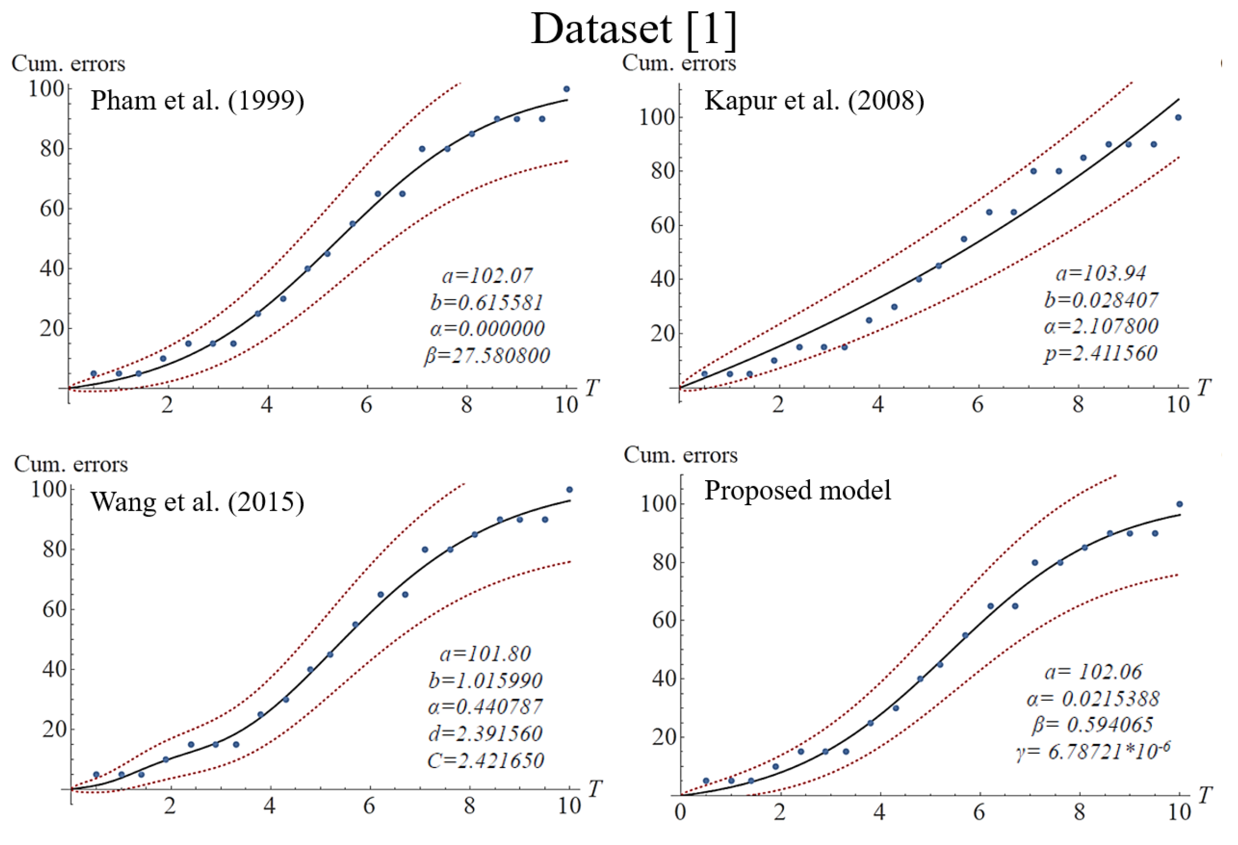
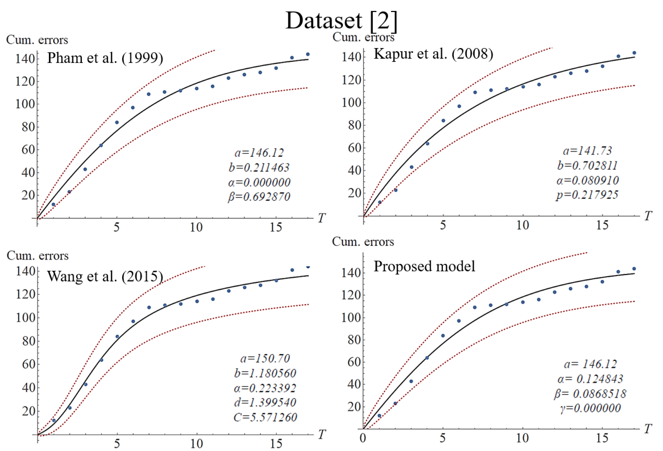
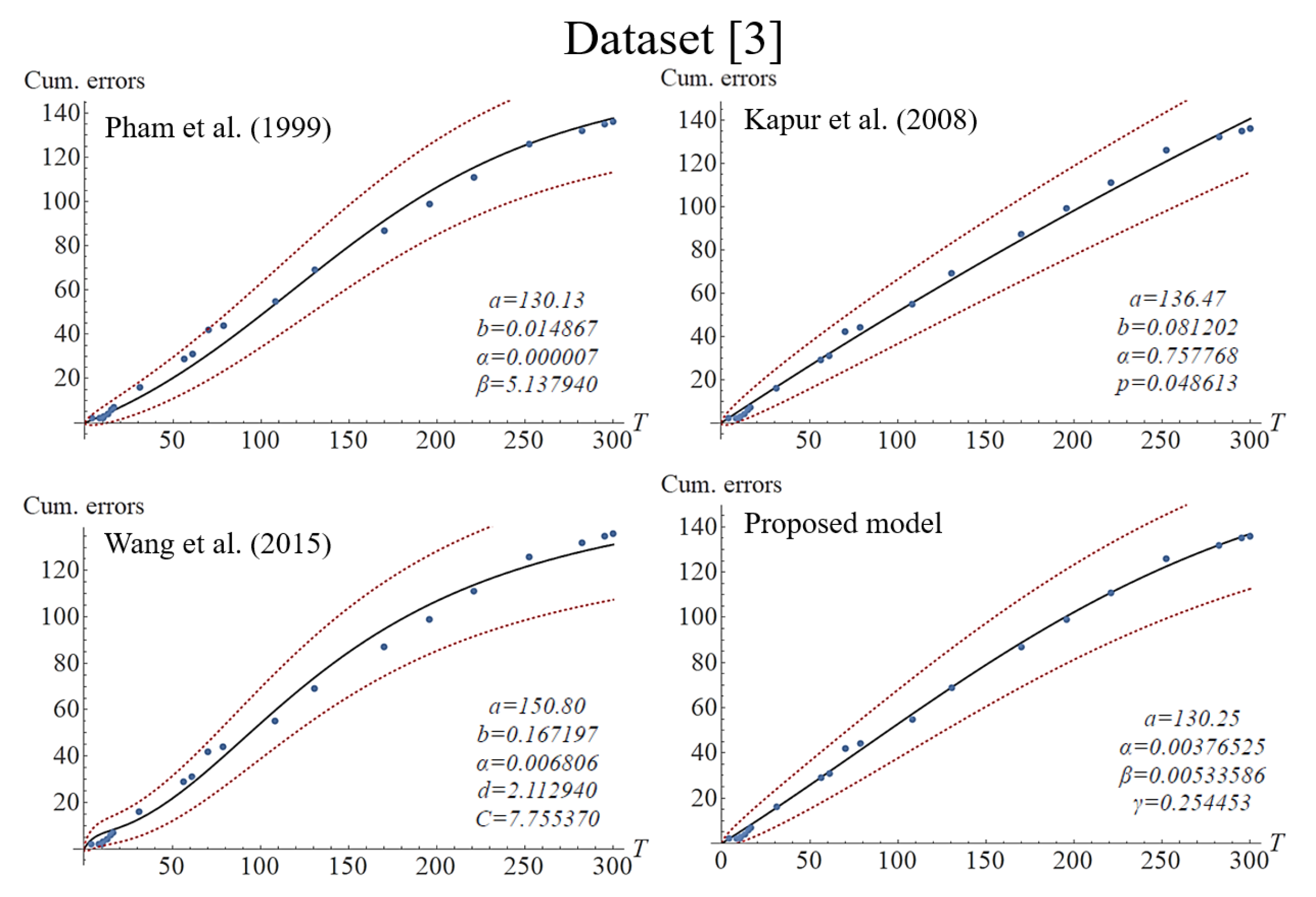
. Figure 1, Figure 2, Figure 3 and Figure 4 present the fitting results of each imperfect debugging SRGM under the different datasets with the traditional CI. In order to fairly investigate the effectiveness of these models, the three most common criteria were chosen. These evaluation criteria were as follows:

(1)

Mean square error (MSE) evaluates the difference between the estimated and true values, i.e., $MSE=\frac{{{\displaystyle \sum }}_{h=1}^n\left(m_h-m\left(t_h\right)\right)}{n-k}$, where $m_h$ is the cumulative number of detected errors from time 0 to $m_h$; $m\left(t_h\right)$ is the cumulative number of detected errors from o to $t_h$ estimated by using the mean value function; $n$ is the number of observations; and $k$ is the number of parameters.

(2)

R-squared explains the variability of data in a model, with a greater value indicating the model has a better fit, and can be given by $Rsq=1-\frac{{{\displaystyle \sum }}_{h=1}^n\left(m_h-m\left(t_h\right)\right)}{{{\displaystyle \sum }}_{h=1}^n\left(m_h-\frac{1}{n}{{\displaystyle \sum }}_{h=1}^n{m}_h\right)}$.

(3)

Akaike information criterion (AIC) [55] is defined as the log-likelihood term penalized by the number of model parameters, which is given by $AIC=n\ast ln\left[\frac{RSS}{n}\right]+2k$.

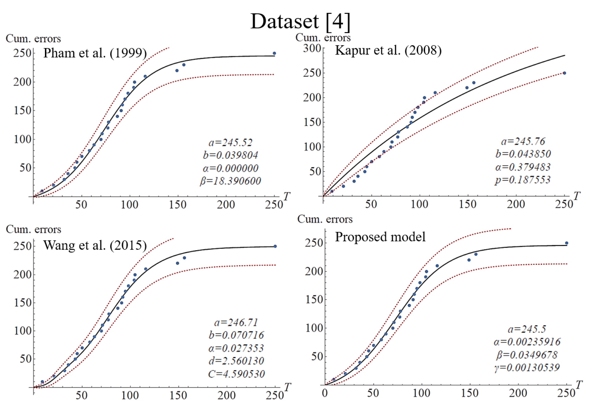
After the analysis of Goodness-of-Fit, it can be seen that the proposed model mostly outperforms the others in the criteria of MSE, R-squared, and AIC under datasets 3 and 4. Moreover, referring to the details in

Table 5. Comparisons of Different Fitting Criteria.

MSE	Data1	Data2	Data3	Data4
Pham et al. (1999) [3]	7.96	44.92	17.35	44.66
Kapur et al. (2008) [9]	42.16	51.86	9.05	463.39
Wang et al. (2015) [12]	6.67	19.22	20.48	41.78
Proposed model	7.96	44.92	4.43	40.91
R-Squared	Data1	Data2	Data3	Data4
Pham et al. (1999) [3]	99.31%	97.22%	99.33%	99.13%
Kapur et al. (2008) [9]	96.37%	96.79%	99.65%	90.92%
Wang et al. (2015) [12]	99.43%	98.81%	99.21%	99.18%
Proposed model	99.31%	97.22%	99.83%	99.20%
AIC	Data1	Data2	Data3	Data4
Pham et al. (1999) [3]	50.55	71.65	66.90	98.16
Kapur et al. (2008) [9]	85.55	74.09	53.24	154.30
Wang et al. (2015) [12]	48.82	59.22	72.39	98.55
Proposed model	50.55	71.65	38.25	96.05

and Figure 2 and Figure 3, we can see that Wang’s model presents an extremely fitting ability for datasets 1 and 2, with R-squared values of 99.43% and 98.81%, respectively. In general, such indicators can measure a model’s performance in adapting to different data patterns, and decision-makers can utilize the applicability of different scenarios to accurately predict the future. However, the situation of overfitting should also be avoided. Examining the bottom-left corners of Figure 2 and Figure 4 for Wang’s model, we can observe the fluctuating curves to fit datasets 1 and 3, which might be due to the phenomenon of overfitting. Overfitting is as an error that occurs in data modeling, in which a particular function may align too closely to a specific dataset but not to other datasets. In other words, a model may overly learn the detail and noise in a specific training dataset. Obviously, the phenomenon of overfitting may negatively impact the performance of a model for new and future datasets. Although the performance of our model may not be superior to that of Wang’s, such overfitting did not show in our model because the proposed model did not show fluctuating curves to fit datasets. It is worth noting that the number of model parameters can influence the fitting ability. In practice, increasing the number of model parameters can effectively improve a model’s flexibility and adaptability. As can be seen in the mean value function of Table 4, Wang’s model has five parameters, while the other models only used four parameters, and therefore Wang’s model can present more flexibility and adaptability than the other models. On the other hand, Kapur’s model shows weak adaptation to S-shaped datasets, perhaps having been developed for a specific scenario. Based on the data presented in Figure 2 and Figure 5, it can be seen that Kapur’s model could only present concave or exponential curves to the S-shaped datasets. Nonetheless, the Kapur model adapts well to the other datasets. In summary, our model presents a better validity of fitness in average cases. In other words, our model’s performance is not inferior to the others. Moreover, since it is easier to comprehend and evaluate our proposed model’s parameters, software testing managers can use them to adjust or modify the values, thereby more accurately predicting the efficiency of a testing scenario that might be changed in the future.

4. Application and Numerical Analysis

Suppose that a business application software provider has developed a commercial software product, and the development of the work is close to the last phase. Therefore, the product manager has to decide the best timing to release the software product. In general, numerous potential software bugs exist in the software, and the number can be estimated by using error seeding methods with consideration of the software scale. In this case, the number of software errors was estimated to be approximately 1650. However, in order to ensure the quality and stability of the software product, testing and debugging works are necessary to satisfy customers’ requirements. Although follow-up service packs can amend the defects of the developed software, customers’ minimal requirement for software reliability is 90%. Consequently, the product manager needs to arrange the appropriate software testing projects and schedules in advance to achieve the objectives of lower cost and higher reliability. However, due to the consideration of the company’s internal human resources, four software testing alternatives can be performed, with the manager choosing the most suitable. After investigation and evaluation by the company’s experts and senior engineers, the information and estimated parameters for the four candidate alternatives can be seen in

Table 6. Related Settings for Candidate Alternatives P1–P4.

Alternative P1	Alternative P2	Alternative P3	Alternative P4
Low-Intensity Manpower	Mediate-Intensity Manpower	Moderate-Intensity Manpower	High-Intensity Manpower
${\widehat{\alpha }}_1$ = 0.25, ${\widehat{\beta }}_1$ = 0.13, ${\widehat{\gamma }}_1$ = 0.06	${\widehat{\alpha }}_2$ = 0.27, ${\widehat{\beta }}_2$ = 0.13, ${\widehat{\gamma }}_2$ = 0.04	${\widehat{\alpha }}_3$ = 0.3, ${\widehat{\beta }}_3$ = 0.18, ${\widehat{\gamma }}_3$ = 0.03	${\widehat{\alpha }}_4$ = 0.32, ${\widehat{\beta }}_4$ = 0.2, ${\widehat{\gamma }}_4$ = 0.03
The initial cost in testing planning, equipment, and preparation works $S{C}_p$ The daily administrative cost per month during the testing period $G{C}_p$
$S{C}_1$ = 5000, $G{C}_1$ = 4500	$S{C}_2$ = 5100, $G{C}_2$ = 4500	$S{C}_3$ = 5200, $G{C}_3$ = 4500	$S{C}_4$ = 8000, $G{C}_4$ = 4500
The estimated ratios of different error types in the system: $q_s$ = 50%, $q_c$ = 30%, $q_d$ = 20%
The costs of removing and correcting different error types under different alternatives
$E{C}_s^1$ = 30, $E{C}_c^1$ = 40, $E{C}_d^1$ = 60	$E{C}_s^2$ = 32, $E{C}_c^2$ = 45, $E{C}_d^2$ = 60	$E{C}_s^3$ = 32, $E{C}_c^3$ = 46, $E{C}_d^3$ = 62	$E{C}_s^4$ = 35, $E{C}_c^4$ = 52, $E{C}_d^4$ = 72
The parameter for the correction time for different error types: ${\xi }_s$ = 5.5, $D^{\left(s\right)}$ = {2.5, 3.1, 0.5, 1.4, 1.5, 0.9, 1.2, 1.1, 0.2, 2.9, 2.3, 0.4}→${\widehat{\theta }}_s$ = 1.75, $E[t_r|{\widehat{\theta }}_s,{\xi }_s]\cong$1.5 h ${\xi }_c$ = 11, $D^{\left(c\right)}$ = {1.3, 4.9, 1.1, 4.2, 2.3, 2.7, 2.4, 1.3, 3.3, 3.1, 2.2, 1.4}→${\widehat{\theta }}_c$ = 2.70, $E[t_r|{\widehat{\theta }}_c,{\xi }_c]\cong$2.5 h ${\xi }_d$ = 15, $D^{\left(d\right)}$ = {4.5, 2.7, 1.5, 3.2, 4.1, 5.3, 3.1, 1.9, 2.5, 4.3, 6.2, 2.9}→${\widehat{\theta }}_d$ = 3.80, $E[t_r|{\widehat{\theta }}_d,{\xi }_d]\cong$3.5 h
The parameters for opportunity cost: ${\omega }_0$ = 1800, ${\omega }_1$ = 2.5 and ${\omega }_2$ = 1.5
The minimal requirement of reliability $R_{mr}$ = 90%, the defined operation time x = 2 h The expected risk cost $RC$ for 1% of system reliability = 3500 The restricted timeline of software release $T_U$ = 20 weeks Testing time for one week is about 44 h The estimated number of all potential errors in the software system $\widehat{a}$ = 1650

. Alternative P1 is devised for a project with low-intensity manpower. The testing team is composed of more junior staff. Even though the efficiency of such alternative testing work is inferior to the others, it can save the costs of removing and correcting different error types. On the contrary, alternative P4 can accelerate the testing work by using high-intensity manpower but it also costs more money due to the requirement of hiring senior staff with experience in testing. Furthermore, each testing staff member performs his/her job in rotation for 44 h per week. Every detected software bug will require different amounts of time to be corrected. The required time for removing bugs is assumed to follow a truncated exponential distribution, and the parameters of the distribution can be obtained by the proposed MLE method. After the calculation using MLE and historical data, the correct times for correcting simple, complex, and difficult errors are estimated to be approximately 1.5, 2.5, and 3.5 h. The manager can use this information to evaluate the related debugging cost. In addition, the risk cost and the opportunity loss are both taken into consideration. The expected risk cost per one percent loss in system reliability is about $3500. The opportunity loss is devised as a time-dependent function, and the parameters are estimated to be ${\omega }_0$ = 1800, ${\omega }_1$ = 2.5, and ${\omega }_2$ = 1.5. The other detailed information can be seen in Table 6.

After calculation employing the proposed model, as shown in

Table 7. The Comparative Results for the Four Alternatives at Different Testing Times.

Weeks	Total Testing Cost				System Reliability
Tp	P1	P2	P3	P4	P1	P2	P3	P4
12	$469,980	$447,576	$395,482	$406,673	57.45%	65.70%	81.56%	86.94%
12.5	$458,701	$437,842	$390,692	$404,546	62.95%	70.73%	85.11%	89.72%
13	$449,157	$430,179	$388,155	$404,438	67.95%	75.17%	88.03%	91.93%
13.5	$441,431	$424,525	$387,557	$405,998	72.44%	79.04%	90.41%	93.69%
14	$435,517	$420,754	$388,598	$408,920	76.42%	82.38%	92.34%	95.07%
14.5	$431,345	$418,705	$391,012	$412,949	79.90%	85.24%	93.90%	96.16%
15	$428,801	$418,204	$394,566	$417,872	82.94%	87.68%	95.14%	97.01%
15.5	$427,751	$419,071	$399,060	$423,518	85.55%	89.73%	96.14%	97.68%
16	$428,047	$421,135	$404,329	$429,748	87.80%	91.47%	96.94%	98.20%
16.5	$429,545	$424,239	$410,237	$436,453	89.72%	92.92%	97.57%	98.60%
17	$432,102	$428,239	$416,670	$443,544	91.36%	94.13%	98.08%	98.91%
17.5	$435,590	$433,011	$423,538	$450,952	92.74%	95.14%	98.48%	99.16%
18	$439,888	$438,444	$430,767	$458,624	93.91%	95.98%	98.79%	99.35%

and Figure 6, the curves of the four alternatives’ expected testing cost show convexity with testing time. Comparing the four alternatives, it can be seen that alternative P3 is more appropriate for the company since its expected testing cost is the lowest of all the other alternatives. Therefore, the manager should adopt alternative P3 and schedule the software release to occur after 13.5 weeks. The software reliability can reach 90.41% and the total expected cost is evaluated to be $387,557. 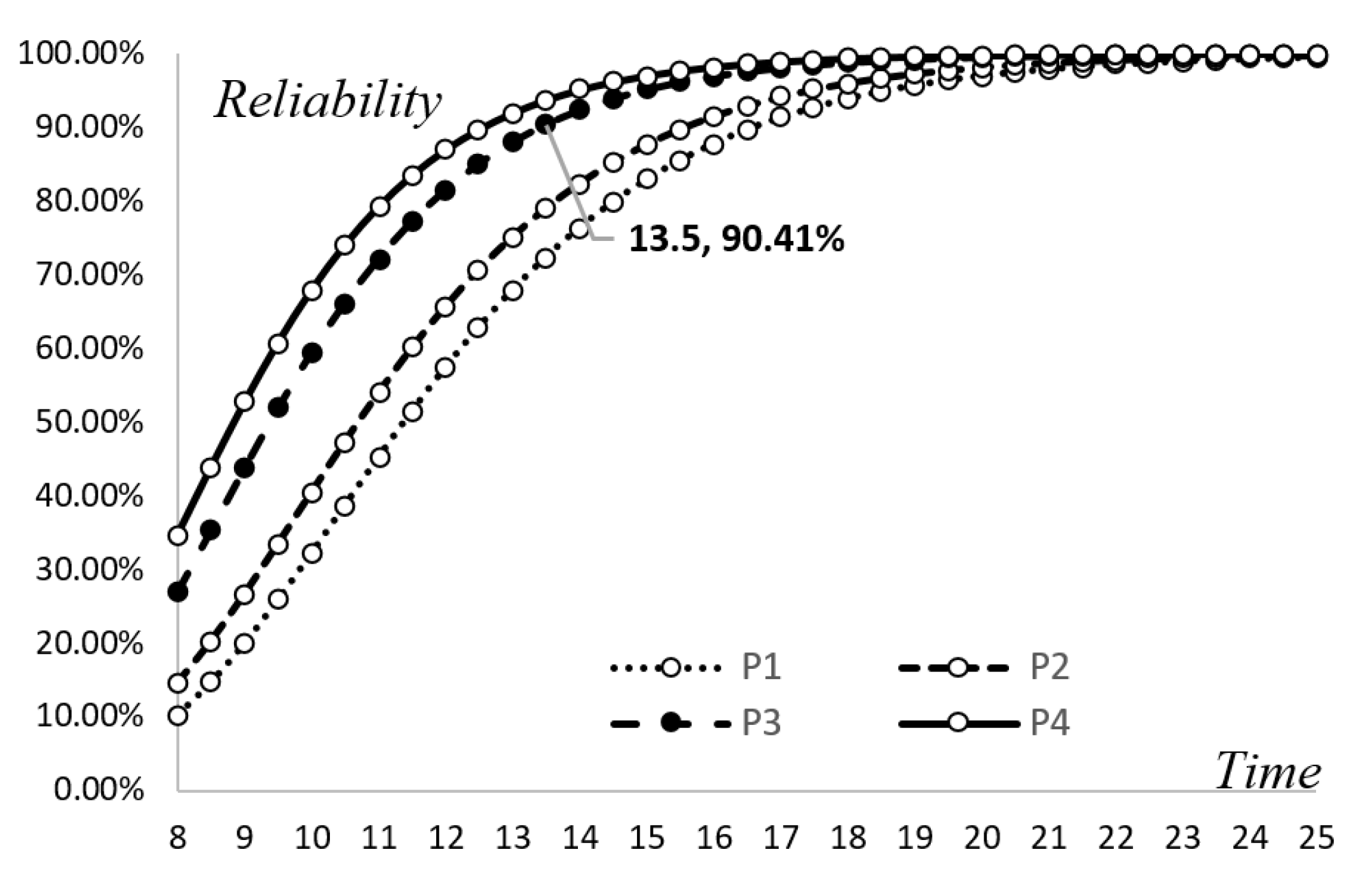With regard to alternatives P1 and P2, the lowest costs are $418,204 and $427,751 at times 15.5 and 15 weeks according to Table 7. However, despite the lower costs, these time points are not feasible solutions since the two alternatives’ software reliability can only reach 85.55% and 87.68% respectively, meaning they cannot satisfy the minimal requirement of software reliability for customers (90%). This minimal requirement would only be reached at 17 and 16 weeks of testing for these two alternatives, respectively. The growth of different alternatives can be seen in Figure 7. Moreover, alternative P4 can rapidly raise the reliability but the related cost is higher than the other alternatives, by about 5–15%. Alternative P3 therefore offers a compromise between reliability and testing cost, and the manager should choose to proceed with the testing work as long as the testing time is within 13.5–18 weeks.

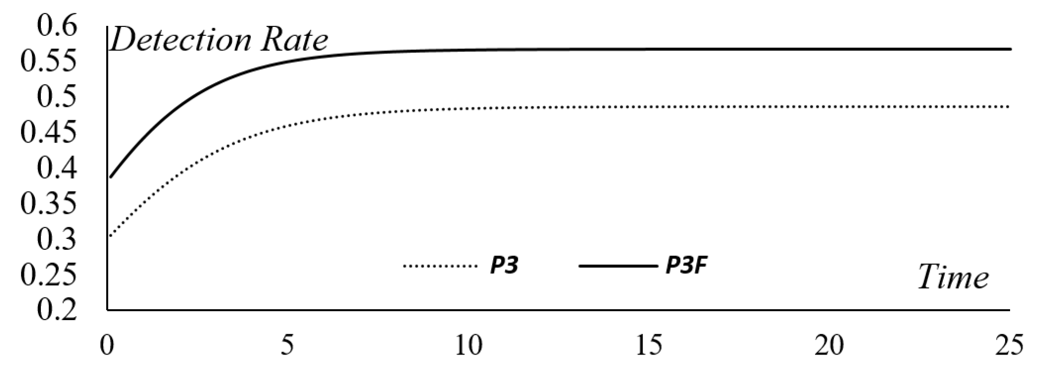
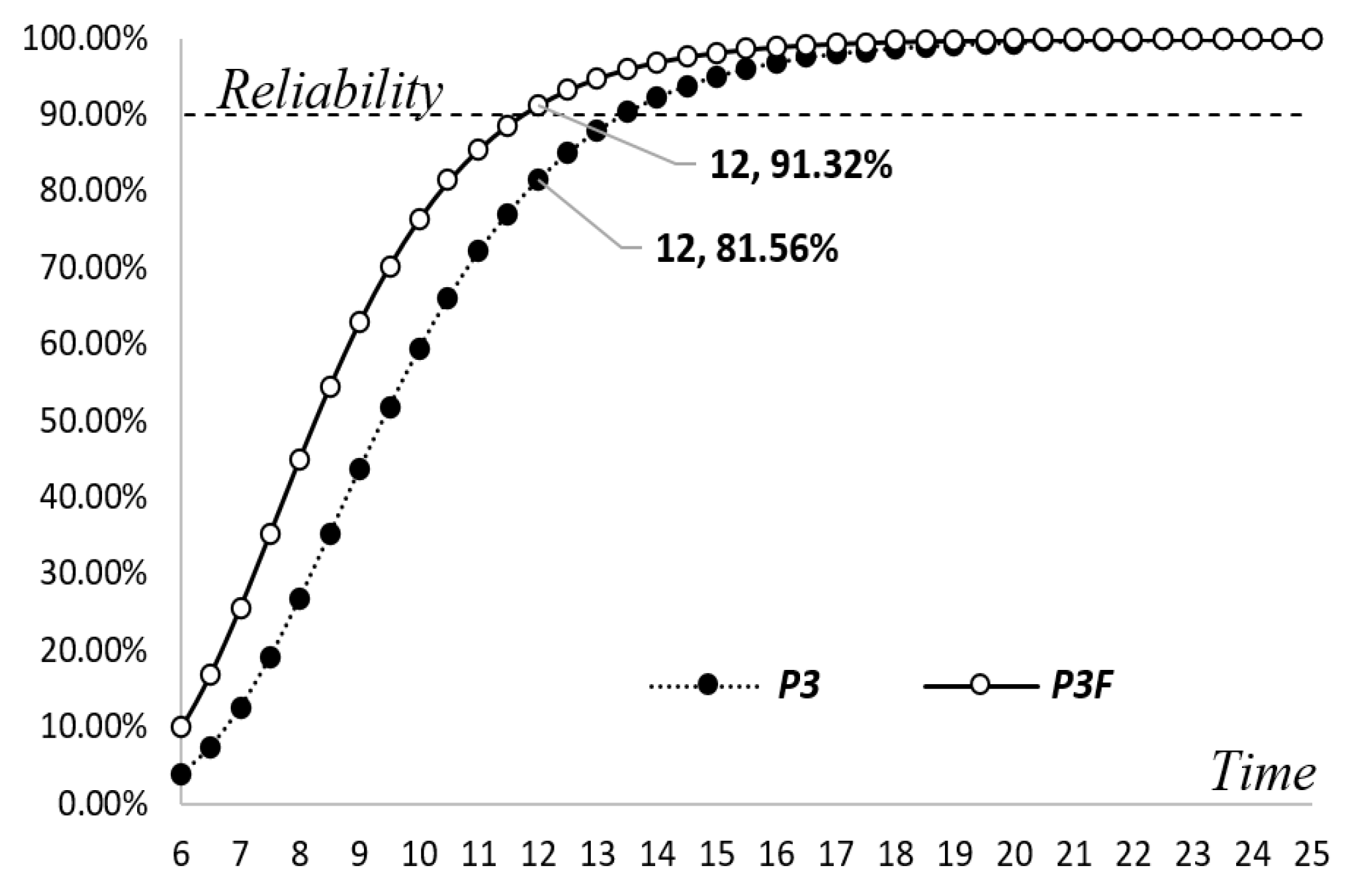
Furthermore, the manager may want to change his/her previous decision in order to release the software product as early as possible. Suppose that the testing work of alternative P3 has proceeded for 5 weeks, and then the manager decides to increase the manpower over the subsequent weeks in order to shorten the original testing schedule, for instance due to commercial competition. The estimated values of the new alternative’s parameters are presented in

Table 8. Related Parameters for the Original and New Alternatives.

Alternative P3	New Alternative (P3F) (after the Changed Testing Environment)
$\mathrm{The} \mathrm{timing} \mathrm{of} \mathrm{the} \mathrm{change} \mathrm{of} \mathrm{testing} \mathrm{alternative} \tau$ = 6 weeks
${\widehat{\alpha }}_3$$=0.3, {\widehat{\beta }}_3$$=0.18, {\widehat{\gamma }}_3$ = 0.03	${\widehat{\alpha }}_3^f$$=0.38, {\widehat{\beta }}_3^f$$=0.18, {\widehat{\gamma }}_3^f$ = 0.04
$S{C}_3$$=5200, G{C}_3$ = 4500	$S{C}_f$$=16,000, G{C}_f$ = 4500
$E{C}_s^3$$=32,E{C}_c^3$$=46,E{C}_d^3$ = 62	$E{C}_s^f$$=45,E{C}_c^f$$=60, E{C}_d^f$ = 70

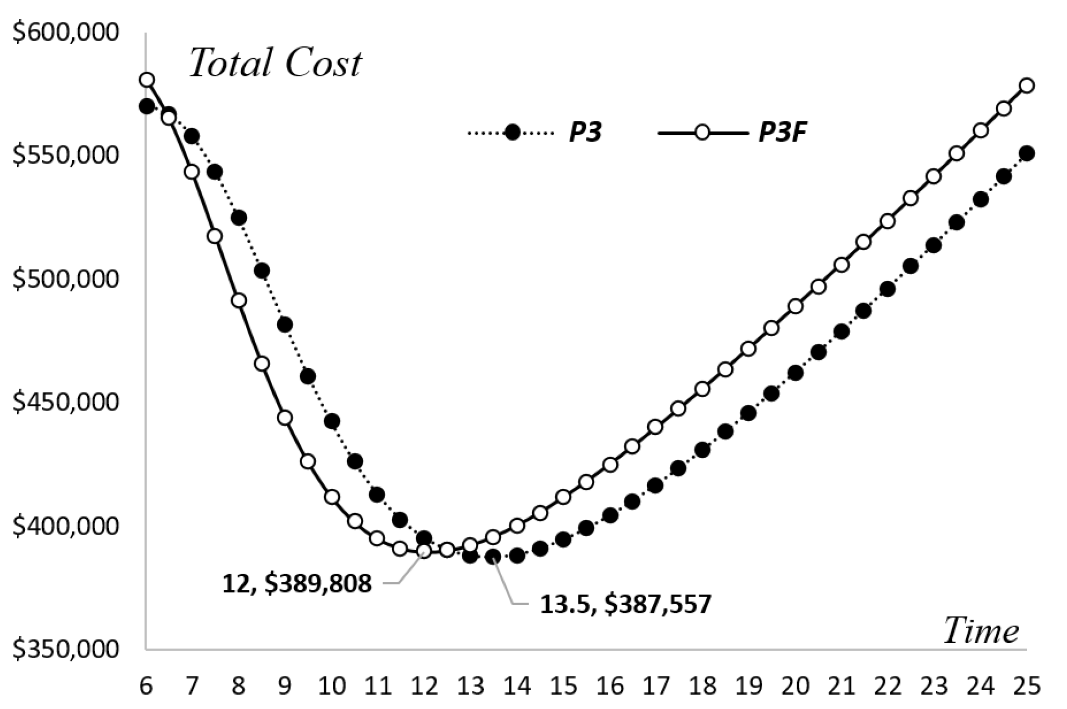
. The learning factor remains the same as before but both the autonomous errors-detected and negligent factors are higher than those in the previous setting. Since the detection rate can be used to investigate the efficiency of testing and debugging, Figure 8 is presented to compare the new alternative with the original one. Although the detection rate of the new alternative is always higher than the original one, it can be seen that the two patterns are similar to each other because the increase in the detection rate with time depends on the size of the learning factor. By employing Equation (30) of the change-point model, the comparative results for the original and new alternatives can be obtained and are presented in

Table 9. Comparative Results for the Former and the New Alternatives.

Weeks	Total Testing Cost		System Reliability
Tp	P3	P3F (after the Changed Environment)	P3	P3F (after the Changed Environment)
10	$442,364	$412,252	59.49%	76.40%
10.5	$426,205	$401,992	66.27%	81.45%
11	$413,024	$395,154	72.21%	85.52%
11.5	$402,837	$391,254	77.28%	88.77%
12	$395,482	$389,808	81.56%	91.32%
12.5	$390,692	$390,369	85.11%	93.32%
13	$388,155	$392,551	88.03%	94.87%
13.5	$387,557	$396,029	90.41%	96.07%
14	$388,598	$400,540	92.34%	96.99%
14.5	$391,012	$405,871	93.90%	97.70%
15	$394,566	$411,855	95.14%	98.24%

and Figure 9 and Figure 10. The optimal timing of software release for the new alternative should be scheduled for the end of the 12th week. The estimated testing cost is approximately equal to $389,808 with a reliability of 91.32%. Although the cost is slightly higher than that of the previous alternative, the duration of the testing can be shorter with no sacrifice in reliability. This is because the increase in the related debugging costs can be offset by the decrease in the opportunity loss. However, if the manager chose to follow the original alternative and did not increase the manpower to raise the testing efficiency, the reliability would only be 81.56% at the end of 12 weeks.

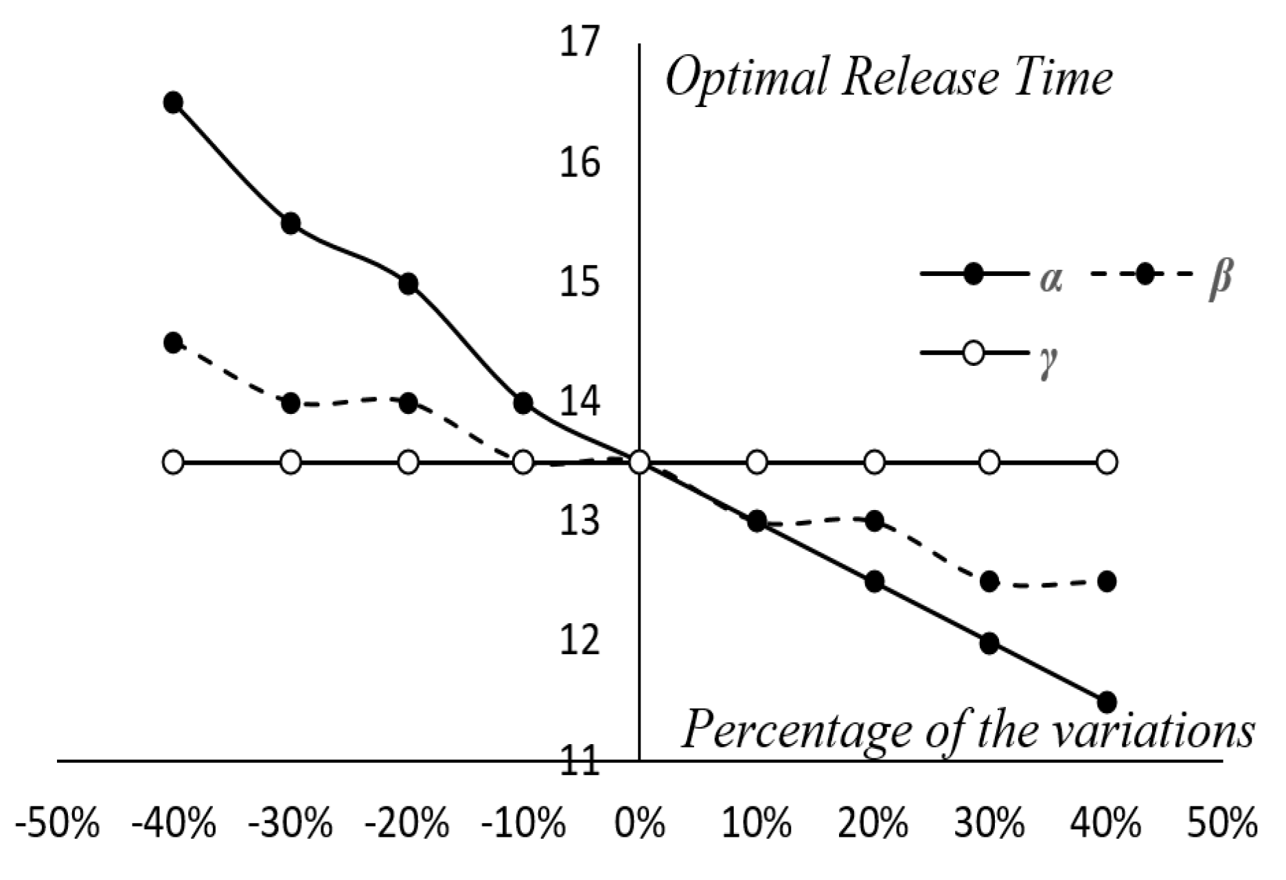
Some additional critical parameters were also considered by performing a sensitivity analysis to investigate their impacts on the total cost and the decision of software release time. Figure 11 presents the impacts of related parameters $\alpha$, $\beta$, $\gamma$, $S{C}_p$, $E{C}_y^p$, and $G{C}_p$ on the total cost. As can be seen in Figure 11, with regard to the model parameters, the cost is more sensitive to $\alpha$ and $\beta$. This means that misestimations of $\alpha$ and $\beta$ will disturb the testing alternative’s budget plan. If the manager underestimated $\alpha$ and $\beta$, it might lead to the overestimation of the testing cost. Furthermore, the misestimation of $\alpha$ and $\beta$ could also influence the company’s software release decision. As can be seen in Figure 12, if the manager overestimated $\alpha$ and $\beta$, he/she will shorten the testing period and rush to release the software. In other words, such a situation may cause dissatisfaction of customers and damage the company’s reputation since the software was released to the market while still unreliable. Moreover, from a different perspective, if the manager wants to increase the efficiency of testing, he/she has to provide more job training to the testing staff in advance, which also increases the cost of educating the testing staff. Although the education investment can raise the values of $\alpha$ and $\beta$, the manager needs to consider the trade-off between any investment in the staff’s skills and the benefit of reducing the cost of reliability improvements. Additionally, the time-dependent administrative cost $G{C}_p$ and the error-correction cost $E{C}_y^p$ would also impact the testing cost. In this case, saving 10% of the error-correction cost can reduce the total testing cost by about 4.5%. The administrative cost is less impactful; saving 10% of the administrative cost may only reduce the total testing cost by about 1.5%. Accordingly, the manager might need to pay attention to how to improve the use of the expenditure for the error-correction works.

5. Conclusions

In this study, we proposed an imperfect debugging software reliability growth model with consideration of human factors and the nature of errors during the debugging process to estimate the related costs and the reliability indicator. Compared with previous models, the estimation of the learning and negligent factors in the proposed model is more intuitive and can be more easily evaluated by internal engineers or domain experts. Furthermore, this study also extended the issue of error classification by considering the impacts of different error types on the system. The expected time required to correct the different types of errors was assumed to obey different truncated exponential distributions. Moreover, in this study, the presented model enables software developers to produce multiple alternatives for a testing project, each with its distinct allocation of human resources. The best alternative can then be identified by utilizing the proposed software release model. These allocations consider debuggers’ learning and negligent factors, which influence the efficiency of software testing in practice. Furthermore, the change-point issue was taken into consideration, i.e., the fact that a software developer may increase manpower and resources so as to accelerate the testing work in practice.

With regard to analyzing the impact of the model parameters $\alpha$, $\beta$, and $\gamma$ on the testing cost, raising $\alpha$ and $\beta$ can help improve debugging efficiency. However, the increase of $\alpha$ and $\beta$ requires more on-the-job training or more senior manpower to achieve. In addition, decreasing the value of parameter $\gamma$ depends on successfully reducing errors in correction work. On-the-job training and online case tools may also help reduce repetitions of the same mistakes. Although education investment is able to raise the values of $\alpha$ and $\beta$, the software developer has to consider the trade-off between any investment in staff’s skills and the given benefit in cost reduction due to reliability improvements. In addition, it should be noted that the optimal time to release a software product to the market is not only a matter of cost, because the software provider must also satisfy the minimal level of software reliability according to the contract or most customers’ requirements. In general, opportunity loss is related to the delay in the software release, and therefore the software developer should carefully estimate the parameters of the opportunity loss from marketing surveys.

Finally, two directions can be considered for future study: (1) The issue of multiple change-points could be taken into consideration since there are many environmental factors that may impact the debugging process at different times, resulting in the scenario of multiple change-points. Furthermore, error classification could also be extended to a function by considering the impacts of errors on the system. The testing staff can correct those errors that have more serious impacts on the system, and the probability distribution can be set to different forms in order to increase the flexibility of applications. (2) The time delay issue in developing a software reliability growth model could also be considered, i.e., the fact that software error correction will consume testing time and might therefore postpone the testing schedule. Most of the related studies have tended to ignore this factor and assume that the time required to correct software errors is zero, potentially leading to errors in the estimation of software reliability. Accordingly, future research might consider the time delay issue to make the model more realistic in practice.