
An Approach to Assessing Spatial Coherence of Current and Voltage Signals in Electrical Networks


1
Energy Research Institute of the Russian Academy of Sciences, 117186 Moscow, Russia
2
Department of Electroenergetics, Power Supply and Power Electronics, Nizhny Novgorod State Technical University, n.a. R.E. Alekseev, 603950 Nizhny Novgorod, Russia
3
Department of Power Supply and Electrical Engineering, Irkutsk National Research Technical University, 664074 Irkutsk, Russia
*
Author to whom correspondence should be addressed.
Mathematics 2022, 10(10), 1768; https://0-doi-org.brum.beds.ac.uk/10.3390/math10101768
Submission received: 5 April 2022
/
Revised: 17 May 2022
/
Accepted: 18 May 2022
/
Published: 22 May 2022
(This article belongs to the Special Issue Model Predictive Control and Optimization for Cyber-Physical Systems)
Abstract
:In the context of energy industry decentralization, electrical networks encounter deviations of power quality indices (PQI), including violations of the sinusoidality of current and voltage signals, which increase errors in the joint digital processing of spatially separated signals in digital devices. This paper addresses specific features of using the concept of spatial coherence in the measurement and digital processing of current and voltage signals. Methods for assessing the coherence of current and voltage signals during synchronized measurements are considered for the case of PQI deviation. The example of a double-ended transmission line fault location (hereafter, DTLFL) demonstrates that the lower the cross-correlation coefficient, the higher the error and the lower the accuracy of calculating the distance to the fault site. The nature of the influence of spatial coherence violations on errors in DTLFL depends on the expression used to calculate the distance to the fault point. The application of a normalized cross-correlation coefficient for finding errors in the digital processing of current and voltage signals, in the case of spatial coherence violation, was substantiated. The influence of interharmonics and noise on errors in DTLFL, in the case of violations of spatial coherence of signals, was investigated. The magnitude of distortions and error in estimating the current and voltage amplitude depends on the ratio between the amplitudes and phases of the fundamental and distorting interharmonics. Filtration of the original and decimated signals based on the discrete Fourier transform eliminates the noise components of the power frequency harmonics.
1. Introduction
The concept of “coherence” is fundamental and is employed in various technical applications related to fluctuating physical quantities. Coherence is used in systems for diagnosing malfunctions of induction motors connected to networks through a frequency-controlled drive [1]. It is also used in photoacoustic systems, to increase contrast and image resolution [2] and to implement multichannel post-filtering [3]. At the same time, “coherence” has specific features, depending on the applied problems, for example, in determining wind loads on lattice frame structures [4], and in electrical networks.
The trend towards the decentralization of the energy industry leads to the massive integration of heterogeneous distributed generation facilities [5], including those based on gas turbine and gas reciprocating generating plants [6], renewable energy sources, and other electrical equipment with elements of power electronics, into power systems [7]. These significantly affect the steady-state conditions, nature and parameters of transient processes, and power quality indices, including the sinusoidality of currents and voltages [8]. Scientific articles pay special attention to assessing the impact of renewable energy sources, in particular photovoltaic plants [9], on PQI, and the impact of PQI on the reliability of power systems [10]. Therefore, the choice of an adequate approach for assessing the coherence of current and voltage signals in synchronized measurements with deviating power quality indices is of great importance.
Spatial coherence plays an important role when using arrays of spatially distributed measurements of distorted current and voltage signals in the network branches and at nodes. Coherence is widely used in the creation of synchronized phasor measurement systems [11,12], relay protection devices [13], and monitoring and control systems [14]. If an array of measurements is considered a matrix of sampled values of a space–time oscillogram, spatial coherence is used to build linear combinations from the spatial samples [15]. MUSIC and ESPRIT are commonly used algorithms for processing spatially coherent signals [16,17].
Consider an array of synchronized current and voltage measurements at n points of the electrical network with the help of n corresponding sensors constituting an n- dimensional vector y(t) = {y(t, ζ1), y(t, ζ2), …, y(t, ζn)} of analytical signals, where the points {ζ1, ζ2, …, ζn} represent spatial location of n sensors [18]. In general, signals can be approximated as:
where A is a matrix of size n × d, and its columns {a(θi): i = 1, 2, …, d} are vectors related with d signals [elements s(t)], which have a corresponding array {θi: i = 1, 2, …, d} of initial phases; n(t) is an additive noise sensor.
The problem for discretized current and voltage signals becomes much more complicated, since they are specified, not in an analytical form, but by corresponding vectors of instantaneous values (or in a complex form), which are a set of samples over the observation interval.
The paper presents an approach for assessing the spatial coherence of current and voltage signals in electrical networks, with the example of two-ended power line fault location. The well-known fault location methods implemented in industrially produced devices for power line fault location do not factor in the coherence of spatially separated signals. This leads to significant errors in calculating the distances to fault points in the case of PQI deviation from the standard values, which increases the time it takes for the operational and repair personnel of electrical networks to locate the power line faults and the time of the power supply disruption for consumers.
This is the first time the normalized cross-correlation coefficient has been used to calculate the distances to the fault sites in power transmission lines, which significantly reduces errors and improves the accuracy of the calculation.
The modeling results proved that the errors in calculations carried out for the power line fault location according to the method proposed in this paper do not exceed 0.2% of the length of the power line. The errors in the calculations made by other known methods can account for several percent of the length of the power line, depending on the voltage class.
The method proposed makes it possible to factor in the complex effect of all PQI deviations using the value of the normalized coefficient of mutual correlation of current and voltage signals. Therefore, even significant PQI deviations will not lead to an increase in the DTLFL calculation error.
This paper aims to substantiate the necessity of using the normalized cross-correlation coefficient to find errors in the digital processing of current and voltage signals in digital devices.
2. Proposed Method for Assessing Spatial Coherence of Current and Voltage Signals in Electrical Networks
Accurate location of a transmission line fault is a complex and significant problem to solve [19]. Its solution makes it possible to considerably reduce the time of fault location in the operating transmission line and the period of emergency recovery work [20,21].
Fault location methods are divided into topographic and remote. Topographic methods involve finding faults in power transmission lines directly during the movement of the repair team along the route of the line. Remote fault location methods suggests using instruments and devices installed at substations and determining the distance to the fault point in the power transmission line using calculation methods [22].
Various fault location methods use transient or steady-state parameters, depending on the type of analyzed information from oscillograms of emergency processes. The methods using transient parameters include, for example, high-frequency fault location methods, while those employing steady-state parameters include low-frequency remote fault location methods [23]. The current and voltage measurements obtained from one or more end of the power transmission line [24] act as an emergency parameters database of the algorithms for fault location in the power transmission line. Depending on the number of measurement points, the fault location methods can be divided into single-ended, double-ended, and multi-ended (centralized).
It is essential for the entities operating power transmission lines to determine with maximum accuracy both the fault site and the power transmission line area to be examined by maintenance personnel, which depends on the magnitude of fault location errors [25].
The spatial coherence feature has not been used to date by any manufacturer of devices for power line fault location and has not been considered in scientific papers addressing fault location in power lines.
It is worth noting that the spatial coherence of current and voltage signals can be neglected in the case of single-ended fault location of power transmission lines, but it is effective to consider it in the cases of double-ended or multi-ended (given power transmission line branches) measurements of currents and voltages, which are used in the joint digital processing of spatially separated signals.
We will consider the case of comparing two sampled voltage signals. Assume that x(t) and y(t) represent the measurement of single signals u(t, ζ) at two different spatial points ζ1 and ζ2:
In a more general case, x(t) and y(t) can represent samples u(t, ζ) at two different points in space at different time instants:
Let us determine the mutual coherence between two space–time oscillograms x(t, ζ) and y(t, ζ).
Let us switch to complex sampled voltage signals with a sampling rate fD = 1/TD, observed on the time interval of N (k = 0, …, N − 1) samples, excluding index ζ. Synchronized presentation of voltage signals with a PQI deviation corresponds to the expressions:
where φ1(k) and φ2(k) are changes in discrete phase-type distribution, ψ1 and ψ2 are initial phases of voltage signals, and f0 is power frequency.
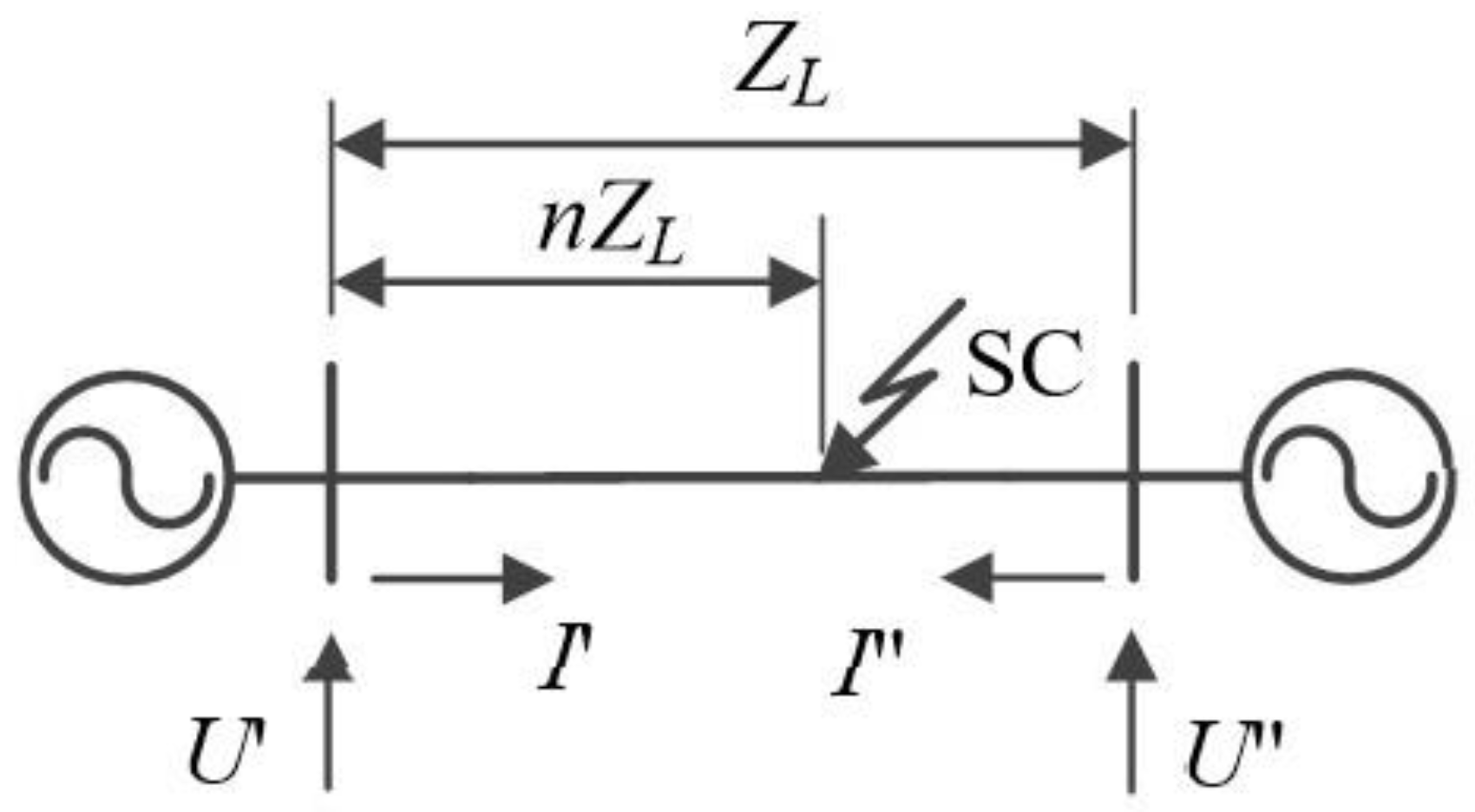
The discrete phase-type distribution φ1(k) and φ2(k) correspond to the discrepancy of the electromotive force (EMF) of power sources, for example, at the ends of a short-circuited power transmission line (Figure 1). In the case of the unsynchronized representation of signals, discrete delays are introduced into Expressions (4) and (5).
Complex vectors (amplitudes) for Expressions (4) and (5) of signals x(k, ψ1) and y(k, ψ2) take the form:
where .
Let us determine the correlation coefficient between discrete signals over an observation interval of N samples:
We write the real part of the number in the form , then Expression (8) can be represented as:
The first group sum in equality (9) can be neglected, since it corresponds to the summation of instantaneous values of a relatively rapidly oscillating function [26]. Then, the final relationship for the complex correlation coefficient takes the form:
In Expression (10), the complex correlation coefficient of the envelopes ρ is equal to
where
while ρ and β are the absolute value and argument of the correlation coefficient.
Using the introduced notation, we transform (10) into the equality
Analysis of Expression (13) shows that, due to phase uncertainty, the correlation coefficient is an undefined value, which does not allow it to be used to compare the considered signals. However, the absolute value of the correlation coefficient is independent of angles ψ1 and ψ2:
Therefore, it can be used to assess the correspondence (degree of similarity) of discrete signals to each other.
Let us define a set of processing operations, to form an absolute value of the correlation coefficient. Assume that the discrete signal x(k) is a reference and known in advance:
Since the correlation coefficient depends on the difference between the initial phases of analyzed signals, in the general case, one can choose a zero initial phase (ψ1 = 0) of signal x(k). Then the expression for the absolute value of the correlation coefficient will take the form:
Let us determine the real part of the complex correlation coefficient:
To estimate the imaginary part of the complex correlation coefficient, we take ψ1 = −π/2
where
and
3. Influence of Spatial Coherence of Current and Voltage Signals on the Accuracy of Double-Ended Fault Location in Power Transmission Lines
3.1. Determination of the Value of the Complex Correlation Coefficient
Current and voltage signals in electrical networks can be affected by distorting interference components [29]. Assume that signal y(k, ψ2) is distorted by discrete-time white noise n(k) with a constant spectral power density N0/2 [26]:
where y(k, ψ2) is determined according to (5), A and ψ2 are parameters of signal y(k, ψ2).
Signals x(k) and xs(k) are determined using Expressions (15) and (19) to calculate the complex correlation coefficient. Note that the discrete random signal yn(k, ψ2) corresponds to the random process with Gaussian distribution and mathematical expectation M[yn(k, ψ2)] = y(k, ψ2).
With the chosen notations, the real and imaginary components of the complex correlation coefficient at a discrete time instant k are determined using the following random variables:
Normal distributions of variables wR and wI correspond to the expressions:
where mwR, mwI and σ2wR, σ2wI are mathematical expectations and variances of random variables wR and wI.
Mathematical expectations mwR, mwI of random variables wR and wI are the results of transformations:
We obtain additional expressions for mathematical expectations:
where ρ and β are determined from equality (12).
We obtain variances of random values wR and wI subject to the equality of energies of signals x(k) and xs(k). Due to the identity of the calculations, we determine variance σ2wR only for signal wR, given that value σ2wR is determined by discrete noise component n(k) of process yn(k, ψ2) (20):
Considering that white noise is δ, i.e., a correlated random process, the mathematical expectation corresponds to the correlation function of the noise process n(k):
Obtain variance of signal wR:
where E is the energy of the quadrature component signal in the calculation of the complex correlation coefficient.
The cross-correlation coefficient of random variables wR and wI corresponds to the expression:
Based on the previously introduced transformations, we obtain:
Bearing in mind Expression (32), we have:
Hence it follows that wR and wI are orthogonal and uncorrelated.
The absolute value of the complex correlation coefficient is obtained by performing operations of linear and nonlinear processing of random variables distributed as per the normal distribution (23) and (24). In this case, the probability density takes a form according to the generalized Rayleigh law [26]:
where I0(·) is a zero-order Bessel function of the first kind; .
3.2. Description of Fault Location in the Power Transmission Line
Fast fault location in 110–220 kV power transmission lines is a crucial objective for power grid companies. The overall time of emergency-related restoration work largely depends on the accuracy of DTLFL [30]. Devices for DTLFL that use calculation methods based on the emergency operating parameters (currents and voltages of individual phases and their components measured during a short circuit) have found widespread use [31,32,33].
The power transmission line fault location devices of various manufacturers implement algorithms for calculating the distance to the fault site [34]. We consider an example of a double-ended transmission line fault location (Figure 1), which does not require synchronized phasor measurements for operation [35].
The distance to the fault location is calculated using measurements of the absolute values of the currents and voltages at the ends of the power transmission line I′, I″, U′, U″, and relationships:
where ZL is the impedance of the power transmission line.
Given that the distance to the fault (SC point) is equal to lSC = n·L, and equating relationships (35) with each other, we arrive at the expression:
where L is the length of the power transmission line.
Expression (36) holds for the components of both negative and zero sequences.
We will consider an example of a fault in a 220 kV power transmission line with L = 120 km. A calculation using Expression (36) was performed using the zero sequence components, and zL = z0 = 3·0.426 = 1.278 Ohm/km. The recorded values of the current and voltage amplitudes were: I′ = 2.0 kA, I″ = 0.56 kA, U′ = 40 kV, U″ = 28 kV.
The above example employs the parameters of emergency conditions (currents and voltages on one of the power line phases at the moment of short circuit), which were actually measured from both ends (at substations) of a real power line.
Then we obtain the distance to the fault site in the power transmission line:
Let us assess the influence of spatial coherence on the DTLFL accuracy. We will sequentially and analytically set expressions for currents and voltages in combination with the impact of the following distorting factors:
- additive current and voltage components in the form of interharmonics of various intensities and spectral ranges;
- a component in the form of white noise in the analyzed frequency spectrum.
The accuracy of the digital processing of signals of the DTLFL should be assessed using the absolute value of the discrete correlation coefficient, which characterizes the signal sinusoidality violation. For the assessment, we assume that a pair of random signals are coherent if the absolute value of the correlation coefficient |ρ| = 1, and incoherent if |ρ| = 0 [36].
We investigate the deviation of the calculated fault location in the power transmission line due to the violations of the sinusoidality of signals I″, U″, and estimate the error in DTLFL.
The sinusoidal signal model for current I′ and voltage U′, with respect to which the correlation coefficient is calculated, will be taken in the form:
With time sequences of discrete signal samples.
The parameters taken to form the discrete values of current i′(n) and voltage u′(n) are I′ = 1A; U′ = 100 V; f0 = 50 Hz; TD = 1/(f0·N) s; N = 80; φ = 0 rad.
4. Investigation of the Influence of Interharmonics and Noise on Errors in DTLFL, in the Case of Violations of the Spatial Coherence of Signals
Assume the additive model for distorted current I″ and voltage U″ of the form:
where M is the number of interharmonics in a spectrum of the sinusoidal signal of current I″ or voltage U″; |Xj|, fj, φj are the amplitude, frequency, and phase of the j-th interharmonic component, respectively.
For simplicity of modeling and analysis of results, we will choose that the current I″ and voltage U″ are distorted by three interhamonics (M = 3, Expression (39)) at frequencies f1 = 75 Hz; f2 = 125 Hz, and f3 = 175 Hz. In doing so, we investigate the effect of relationships between amplitudes |Xj| and phases φj of interharmonics on the correlation coefficient of signals and the respective errors in DTLFL.
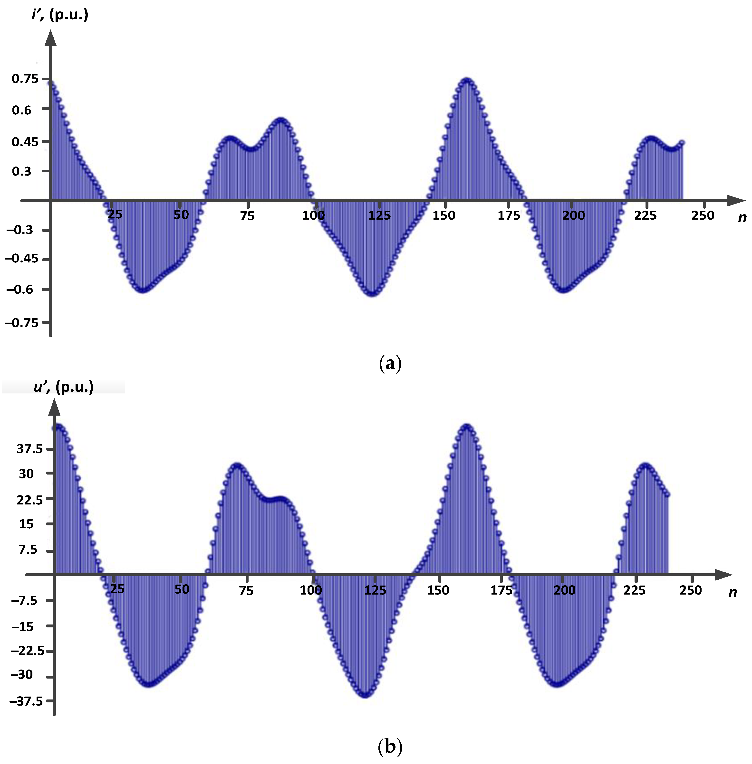
Let for the amplitudes and phases of the interharmonics, being parts of the discrete values of current i′(n) and voltage u′(n), there be the following relationship |Xi1| = 0.15·I″; |Xi2| = 0.1·I″; |Xi3| = 0.15·I″; |Xu1| = 0.1·U″; |Xu2| = 0.15·U″; |Xu3| = 0.1·U″; φi1 = 0 rad; φi2 = (π/6) rad; φi3 = (π/4) rad; φu1 = (−π/6) rad; φu2 = (−π/4) rad; φu3 = 0 rad. Oscillograms of current and voltage corresponding to the specified amplitude–phase relationships of sinusoidal signals of current i′(n) and voltage u′(n) are presented in Figure 2. Modeling was carried out in Mathcad software.
We estimate the amplitudes of current I″ and voltage U″ by simulating the filtering process with the measuring element of the device for DTLFL, by performing a discrete Fourier transform (DFT) for the distorted harmonics of current and voltage at power frequency (Figure 2):
The results of the modeling (calculations) with the use of (40), (41) show that the amplitudes of the measured fundamental harmonic of current i″(n) and voltage u″(n) signals (Figure 2) correspond to the values Im″ = |Si| = 0.547 kA and Um″ = |Su| = 30.223 kV. Thus, the DFT of a distorted sinusoidal power-frequency signal did not completely filter out the set of interharmonics and led to a distortion of the estimation results for the parameters of current I″ and voltage U″. The magnitude of distortion and error in estimating the current and voltage amplitude depends on the relationship between the amplitudes and phases of the fundamental and distorting interharmonics [37].
The violations of the spatial coherence of currents and voltages are assessed using the absolute value of the correlation coefficient (Expression (14)). We use its normalized value, which in practical calculations for the sets of instantaneous values of currents and voltages i′(n), i″(n), u′(n), u″(n) takes the form:
where
Given the obtained values Im″ and Um″, we calculate an error in the double-ended power transmission line fault location under a violated spatial coherence of the current and voltage signals. We substitute amplitudes Im″ and Um″ into Expression (36) to calculate the distance to the fault site in a power transmission line (Figure 1):
We determine the error in the DTLFL, caused by violations of spatial coherence, in the form:
Its value for the considered example of combinations of interharmonic parameters is equal to Δ = −0.19 km or 0.16% (calculation 1 in Table 1).
Table 1 shows the results of the simulation modeling and calculation of the double-ended fault location errors for various amplitude–phase relationships of the current and voltage interharmonics.
The modeling results show that the error in the calculations of the power line fault location according to the proposed method, given the normalized cross-correlation coefficient, does not exceed 0.2% of the length of the power transmission line. The errors in the calculations by other known methods can reach several percent of the length of the power line, depending on the voltage classes (Table 1).
The analysis of modeling and calculating errors in double-ended transmission line fault location with various amplitude–phase relationships of the current and voltage interharmonics has shown the following:
- errors in DTLFL depend on violations of sinusoidality of current and voltage signals, and the amplitude–phase relationships of interharmonics that are part of the distorted signals. The amplitude–phase relationships of interharmonics can both decrease and increase the values of the amplitudes of current I″ and voltage U″. With the same amplitude relationships, changes in the phase ratios lead to significant differences in errors in DTLFL. A 1.5-fold decline in the amplitudes of interharmonics at the same phase relationships results in a disproportionate decrease in the error in DTLFL;
- the discrete Fourier transform, in measuring elements of digital devices, provides complete suppression of multiple harmonics. However, when analyzing the spatial coherence of discrete currents and voltages, one should take into account the influence of interharmonics, the aperiodic component, and noise on the process of digital signal processing;
- the cross-correlation coefficient can be chosen as a numerical characteristic that makes it possible to estimate the magnitude of the distortion of the current and voltage signals of power frequency and to characterize a violation of spatial coherence. The smaller the cross-correlation coefficient, the greater the error in DTLFL will be;
- the nature of the influence of violations of spatial coherence on errors in DTLFL depends on the expression used to calculate the distance to the site of a power line fault. Consequently, different algorithms designed for DTLFL have their own inherent robustness to violations of spatial coherence.
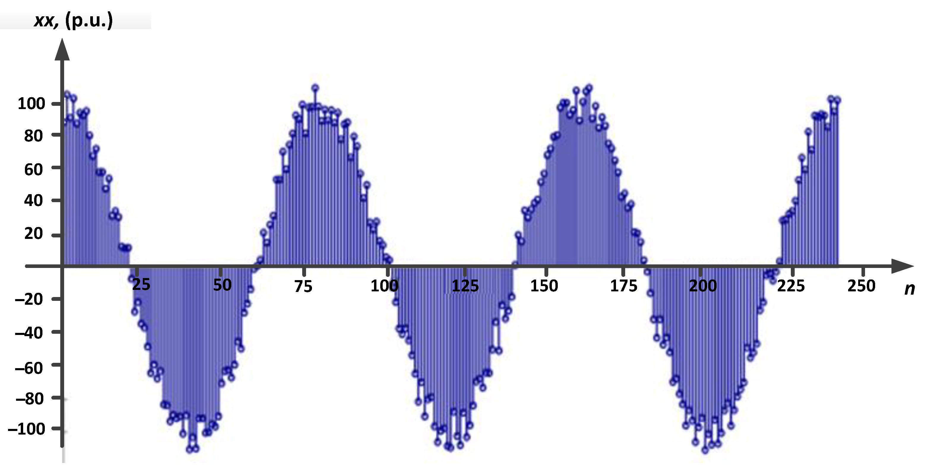
Let us investigate the effect of noise on the errors in DTLFL in the case of a violation of spatial coherence of current and voltage signals. We take a mathematical model of current and voltage signals, in the form of a mixture of signal x(n) (Expression (38)) and noise distortions in the analyzed frequency band (Figure 3):
where g(n) are random instantaneous values of the noise component.
The results of modeling (calculations) showed that DFT filtering of the original and decimated signals effectively eliminates noise components from the power frequency harmonic.
Deviations of the estimates of current I″ and voltage U″ amplitudes depend on the noise intensity, but account for no more than a few percent, which is within the permissible measurement error. Calculation of the normalized cross-correlation coefficient for signals, distorted and undistorted by noise, has shown that its value is close to unity.
5. Conclusions
Joint digital processing of spatially separated signals should factor in spatial coherence, to minimize errors in estimating the parameters of currents and voltages of power frequency.
A normalized cross-correlation coefficient is appropriate for determining the extent of the current and voltage sinusoidality distortion due to violations of spatial coherence.
The example of a DTLFL indicated that the smaller the cross-correlation coefficient (a significant change in spatial coherence of sinusoidal signals), the higher the error and the lower the accuracy of calculating the distance to the fault site.
The nature of the influence of spatial coherence violations on the errors in DTLFL depends on the expression used to calculate the distance to the fault point, which is why various algorithms designed to detect fault location in power transmission lines have their own inherent robustness to violations of spatial coherence.
The modeling results showed that the error in the calculations of the power line fault location according to the proposed method, given a normalized cross-correlation coefficient, does not exceed 0.2% of the length of the power transmission line. The errors in the calculations by other known methods can reach several percent of the length of the power line, depending on the voltage classes of the line.
Author Contributions
Conceptualization, P.I. and A.K.; methodology, S.F.; software, P.I.; validation, K.S. and S.F.; formal analysis, A.K.; data curation, K.S.; writing—original draft preparation, P.I.; writing—review and editing, K.S.; visualization, P.I.; supervision, A.K.; project administration, S.F. All authors have read and agreed to the published version of the manuscript.
Funding
This research received no external funding.
Institutional Review Board Statement
Not applicable.
Informed Consent Statement
Informed consent was obtained from all subjects involved in the study.
Data Availability Statement
Data sharing not applicable. No new data were created or analyzed in this study. Data sharing is not applicable to this article.
Conflicts of Interest
The authors declare no conflict of interest. The funders had no role in the design of the study; in the collection, analyses, or interpretation of data; in the writing of the manuscript, or in the decision to publish the results.
Nomenclature
| fD | sampling frequency |
| TD | sampling time (step) |
| f0 | power frequency of the network |
| |Xj|, fj, φj | amplitude, frequency and phase of the j-th interharmonic component |
| N | observation interval |
| Ρ | absolute value of the correlation coefficient |
| Β | argument of the correlation coefficient |
| yn | discrete random signal |
| mwR, mwI | mathematical expectations of random variables wR and wI |
| σ2wR, σ2wI | variances of random variables wR and wI |
| δ | white noise |
| E | signal energy |
| I0(·) | zero-order Bessel function of the first kind |
| I′, U′ | measured current and voltage magnitudes at the beginning of the power line |
| I″, U″ | measured current and voltage magnitudes at the end of the power line |
| Im, Um | current and voltage magnitudes obtained by simulation modeling |
| L | power transmission line length |
| z0 | zero sequence resistance of the power line |
| USC | phase voltage at the fault site |
| lSC | distance to the short circuit site |
| M | number of interharmonics in the spectrum of a sinusoidal current or voltage signal |
| g(n) | random instantaneous values of a noise component |
References
- Khan Shabbir, M.N.S.; Liang, X. A DFFT and Coherence Analysis-Based Fault Diagnosis Approach for Induction Motors Fed by Variable Frequency Drives. In Proceedings of the 2020 IEEE Canadian Conference on Electrical and Computer Engineering (CCECE), London, ON, Canada, 26–29 April 2020. [Google Scholar]
- Graham, M.T.; Lediju Bell, M.A. Photoacoustic Spatial Coherence Theory and Applications to Coherence-Based Image Contrast and Resolution. IEEE Trans. Ultrason. Ferroelectr. Freq. Control 2020, 67, 2069–2084. [Google Scholar] [CrossRef] [PubMed]
- Hu, J.S.; Lee, M.T. Multi-channel post-filtering based on spatial coherence measure. Signal Process. 2014, 105, 338–349. [Google Scholar] [CrossRef]
- Li, F.; Zou, L.; Songa, J.; Liang, S.; Chen, Y. Investigation of the spatial coherence function of wind loads on lattice frame structures. J. Wind Eng. Ind. Aerodyn. 2021, 215, 104675. [Google Scholar] [CrossRef]
- Mehigana, L.; Deanea, J.P.; Gallachóira, B.P.Ó.; Bertsch, V. A review of the role of distributed generation (DG) in future electricity systems. Energy 2018, 163, 822–836. [Google Scholar] [CrossRef]
- Ilyushin, P.V.; Kulikov, A.L.; Suslov, K.V.; Filippov, S.P. Consideration of Distinguishing Design Features of Gas-Turbine and Gas-Reciprocating Units in Design of Emergency Control Systems. Machines 2021, 9, 47. [Google Scholar] [CrossRef]
- Buchholz, B.M.; Styczynski, Z. Smart Grids-Fundamentals and Technologies in Electricity Networks; Springer: Berlin/Heidelberg, Germany; New York, NY, USA; Dordrecht, The Netherlands; London, UK, 2014; p. 396. [Google Scholar]
- Arranz-Gimon, A.; Zorita-Lamadrid, A.; Morinigo-Sotelo, D.; Duque-Perez, O. A review of total harmonic distortion factors for the measurement of harmonic and interharmonic pollution in modern power systems. Energies 2021, 14, 6467. [Google Scholar] [CrossRef]
- Silva, E.N.M.; Rodrigues, A.B.; Da Guia Da Silva, M. Stochastic assessment of the impact of photovoltaic distributed generation on the power quality indices of distribution networks. Electr. Power Syst. Res. 2016, 135, 59–67. [Google Scholar] [CrossRef]
- Savina, N.V.; Myasoedov, Y.V.; Myasoedova, L.A. Influence of quality of the electric energy on reliability of electrical supply systems. In Proceedings of the 2018 International Multi-Conference on Industrial Engineering and Modern Technologies (FarEastCon), Vladivostok, Russia, 2–4 October 2018; p. 8602690. [Google Scholar]
- Phadke, A.G.; Thorp, J.S. Synchronized Phasor Measurements and Their Applications; Springer: New York, NY, USA, 2008. [Google Scholar]
- Kezunovic, M.; Meliopoulos, S.; Venkatasubramanian, V.; Vittal, V. Application of Time-Synchronized Measurements in Power System Transmission Networks; Springer: New York, NY, USA, 2014. [Google Scholar]
- Wide Area Protection & Control Technologies; CIGRE Working Group B5.14; CIGRE: Paris, France, 2016.
- Arghandeh, R.; Brady, K.; Brown, M.; Cotter, G.R.; Deka, D.; Hooshyar, H.; Jamei, M.; Kirkham, H.; McEachern, A.; Mehrmanesh, L.; et al. Synchrophasor Monitoring for Distribution Systems: Technical Foundations and Applications; A White Paper by the NASPI Distribution Task Team NASPI-2018-TR-001; U.S. Department of Energy: Washington, DC, USA, 2018.
- Ribeiro, P.F.; Duque, C.A.; da Silveira, P.M.; Cerqueira, A.S. Power Systems Signal Processing for Smart Grids; John Wiley & Sons: Michigan, MI, USA, 2014. [Google Scholar]
- Marple, S.L. Digital Spectral Analysis: With Applications; Prentice Hall: Englewood Cliffs, NJ, USA, 1987. [Google Scholar]
- Gardner, W.A. Introduction to Random Processes with applications to Signal and Systems. In With Applications to Signals & Systems; McGraw Hill: New York, NY, USA, 1990; p. 560. [Google Scholar]
- Shushpanov, I.; Suslov, K.; Ilyushin, P.; Sidorov, D. Towards the flexible distribution networks design using the reliability performance metric. Energies 2021, 14, 6193. [Google Scholar] [CrossRef]
- Shalyt, G.M.; Aizenfeld, A.I.; Maly, A.S. Power Line Fault Location Based on the Emergency Parameters; Energoatomizdat: Moscow, Russia, 1983; p. 208. [Google Scholar]
- Saha, M.M.; Izykowski, J.; Rosolowski, E. Fault Location on Power Networks; Springer: London, UK, 2010; p. 437. [Google Scholar]
- Izykowsky, J. Fault Location on Power Transmission Line; Springer: Berlin/Heidelberg, Germany, 2008; p. 221. [Google Scholar]
- Visyashchev, A.N. Devices and Methods for Locating Faults on Power Lines: Textbook in 2 Parts—Part 1; ISTU Publishing House: Irkutsk, Russia, 2001; p. 188. [Google Scholar]
- Schweitzer, E.O. A review of impedance-based fault locating experience. In Proceedings of the 14th Annual Iowa–Nebraska System Protection Seminar, Omaha, NE, USA, 16 October 1990; pp. 1–31. [Google Scholar]
- Kezunovic, M.; Perunicic, B. Fault Location: Wiley Encyclopedia of Electrical and Electronics Terminology; John Wiley & Sons: New York, NY, USA, 1999; Volume 7, pp. 276–285. [Google Scholar]
- Rebizant, W.; Szafran, J.; Wiszniewski, A. Digital Signal Processing in Power System Protection and Control; Springer: New York, NY, USA, 2011; p. 316. [Google Scholar]
- Shirman, Y.D.; Baghdasaryan, S.T.; Malyarenko, A.S. Radioelectronic Systems: Fundamentals of Construction and Theory: Handbook. Radioengineering 2007, 512. (In Russian) [Google Scholar]
- Shneerson, E.M. Digital Relay Protection; Energoatomizdat: Moscow, Russia, 2007; p. 549. (In Russian) [Google Scholar]
- Falshina, V.A.; Kulikov, A.L. Algorithms for simplified digital filtering of electrical signals of industrial frequency. Ind. Energy 2012, 5, 39–46. (In Russian) [Google Scholar]
- Ilyushin, P.V. Analysis of the specifics of selecting relay protection and automatic (RPA) equipment in distributed networks with auxiliary low-power generating facilities. Power Technol. Eng. 2018, 51, 713–718. [Google Scholar] [CrossRef]
- Arzhannikov, E.A.; Lukoyanov, V.Y.; Misrikhanov, M.S. Determining the Location of a Short Circuit on High-Voltage Power Lines; Shuin, V.A., Ed.; Energoatomizdat: Moscow, Russia, 2003; p. 272. (In Russian) [Google Scholar]
- Obalin, M.D.; Kulikov, A.L. Application of adaptive procedures in algorithms for determining the location of damage to power lines. Ind. Energy 2013, 12, 35–39. (In Russian) [Google Scholar]
- Sheta, A.N.; Abdulsalam, G.M.; Eladl, A.A. Online tracking of fault location in distribution systems based on PMUs data and iterative support detection. Int. J. Electr. Power Energy Syst. 2021, 128, 106793. [Google Scholar] [CrossRef]
- Abbas, A.K.; Hamad, S.; Hamad, N.A. Single line to ground fault detection and location in medium voltage distribution system network based on neural network. Indones. J. Electr. Eng. Comput. Sci. 2021, 23, 621. [Google Scholar] [CrossRef]
- Shabalov, M.Y.; Zhukovskiy, Y.L.; Buldysko, A.D.; Gil, B.; Starshaia, V.V. The influence of technological changes in energy efficiency on the infrastructure deterioration in the energy sector. Energy Rep. 2021, 7, 2664–2680. [Google Scholar] [CrossRef]
- Kulikov, A.L.; Loskutov, A.A.; Ilyushin, P.V. High-performance sequential analysis in grid automated systems of distributed-generation areas. Russ. Electr. Eng. 2021, 92, 90–96. [Google Scholar] [CrossRef]
- Cook, C.E.; Bernfeld, M. Radar Signals; Academic Press: Cambridge, MA, USA, 1967; p. 531. [Google Scholar]
- Lavrik, A.; Zhukovskiy, Y.; Tcvetkov, P. Optimizing the Size of Autonomous Hybrid Microgrids with Regard to Load Shifting. Energies 2021, 14, 5059. [Google Scholar] [CrossRef]
Figure 1.
Simplified single-line diagram of a power transmission line in the case of a short circuit (SC).
Figure 1.
Simplified single-line diagram of a power transmission line in the case of a short circuit (SC).

Figure 2.
Sinusoidal signals distorted by interharmonics: (a) current; (b) voltage.

Figure 3.
Oscillogram of a sinusoidal current (voltage) signal distorted by noise.


Table 1.
Errors in power line fault location in the case of a violated spatial coherence of the current and voltage signals.
Table 1.
Errors in power line fault location in the case of a violated spatial coherence of the current and voltage signals.
| Calculation Options | Amplitude–Phase Relationships of Current and Voltage Interharmonics | Normalized Current (Voltage) Correlation Coefficient | Error in Power Line Fault Location Δ under Violated Spatial Coherence | |||||||||||
|---|---|---|---|---|---|---|---|---|---|---|---|---|---|---|
| |Xi1| (I″) | |Xi2| (I″) | |Xi3| (I″) | φi1 | φi2 | φi3 | |Xu1| (U″) | |Xu2| (U″) | |Xu3| (U″) | φu1 | φu2 | φu3 | |||
| 1. | 0.15 | 0.1 | 0.15 | 0 | π/6 | π/4 | 0.1 | 0.15 | 0.1 | −π/6 | −π/4 | 0 | 0.973 (0.985) | −0.19 km (0.16%) |
| 2. | 0.15 | 0.15 | 0.15 | π | π | π | 0.15 | 0.15 | 0.15 | −π | −π | −π | 0.967 (0.967) | 0.176 km (0.15%) |
| 3. | 0.15 | 0.15 | 0.15 | π | π | π | 0.15 | 0.15 | 0.15 | 0 | 0 | 0 | 0.967 (0.969) | −0.0165 km (0.014%) |
| 4. | 0.15 | 0.15 | 0.15 | 0 | 0 | 0 | 0.15 | 0.15 | 0.15 | 0 | 0 | 0 | 0.969 (0.969) | −0.491 km (0.41%) |
| 5. | 0.15 | 0.15 | 0.15 | π/2 | π/2 | π/2 | 0.15 | 0.15 | 0.15 | 0 | 0 | 0 | 0.977 (0.969) | 4.063 km (3.39%) |
| 6. | 0.15 | 0.15 | 0.15 | −π/2 | −π/2 | −π/2 | 0.15 | 0.15 | 0.15 | 0 | 0 | 0 | 0.989 (0.969) | −4.011 km (3.34%) |
| 7. | 0.1 | 0.1 | 0.1 | −π/2 | −π/2 | −π/2 | 0.1 | 0.1 | 0.1 | 0 | 0 | 0 | 0.995 (0.986) | −2.701 km (2.25%) |
| 8. | 0.1 | 0.1 | 0.1 | −π/2 | −π/2 | −π/2 | 0.1 | 0.1 | 0.1 | π/2 | π/2 | π/2 | 0.995 (0.991) | −1.567 km (1.31%) |
| 9. | 0.1 | 0. | 0.1 | −π/2 | −π/2 | −π/2 | 0.1 | 0.1 | 0.1 | 3π/2 | 3π/2 | 3π/2 | 0.995 (0.995) | −3.67 km (3.06%) |
| 10. | 0.1 | 0.1 | 0.1 | −π/2 | −π | −3π/2 | 0.1 | 0.1 | 0.1 | 3π/2 | 3π/2 | 3π/2 | 0.988 (0.995) | −2.21 km (1.84%) |
Publisher’s Note: MDPI stays neutral with regard to jurisdictional claims in published maps and institutional affiliations. |
© 2022 by the authors. Licensee MDPI, Basel, Switzerland. This article is an open access article distributed under the terms and conditions of the Creative Commons Attribution (CC BY) license (https://creativecommons.org/licenses/by/4.0/).
Share and Cite
MDPI and ACS Style
Ilyushin, P.; Kulikov, A.; Suslov, K.; Filippov, S. An Approach to Assessing Spatial Coherence of Current and Voltage Signals in Electrical Networks. Mathematics 2022, 10, 1768. https://0-doi-org.brum.beds.ac.uk/10.3390/math10101768
AMA Style
Ilyushin P, Kulikov A, Suslov K, Filippov S. An Approach to Assessing Spatial Coherence of Current and Voltage Signals in Electrical Networks. Mathematics. 2022; 10(10):1768. https://0-doi-org.brum.beds.ac.uk/10.3390/math10101768
Chicago/Turabian StyleIlyushin, Pavel, Aleksandr Kulikov, Konstantin Suslov, and Sergey Filippov. 2022. "An Approach to Assessing Spatial Coherence of Current and Voltage Signals in Electrical Networks" Mathematics 10, no. 10: 1768. https://0-doi-org.brum.beds.ac.uk/10.3390/math10101768
Note that from the first issue of 2016, this journal uses article numbers instead of page numbers. See further details here.