Topological Data Analysis with Spherical Fuzzy Soft AHP-TOPSIS for Environmental Mitigation System

Abstract

The idea of spherical fuzzy soft set (SFSS) is a new hybrid model of a soft set (SS) and spherical fuzzy set (SFS). An SFSS is a new approach for information analysis and information fusion, and fuzzy modeling. We define the concepts of spherical-fuzzy-soft-set topology (SFSS-topology) and spherical-fuzzy-soft-set separation axioms. Several characteristics of SFSS-topology are investigated and related results are derived. We developed an extended choice value method (CVM) and the AHP-TOPSIS (analytical hierarchy process and technique for the order preference by similarity to ideal solution) for SFSSs, and presented their applications in multiple-criteria group decision making (MCGDM). Moreover, an application of the CVM is presented in a stock market investment problem and another application of the AHP-TOPSIS is presented for an environmental mitigation system. The suggested methods are efficiently applied to investigate MCGDM through case studies.

1. Introduction

The data in classical analysis often carry interesting geometric and topological properties. Characterizing the complexities of such properties with efficient models, algorithms, and tools is a challenging problem that requires new mathematical modeling. Classical topology has expanded by drawing inspiration from classical analysis and it has a number of applications in domains such as learning algorithms [1,2], data analysis [3], machine learning, large data, data mining [4,5], quantum gravity, and cosmological models [6]. Additionally, the term “topology” refers to the relationship between geometric objects and features, and can be used to characterize certain spatial functions and to comprehend data sets with improvements in product quality control and data integrity. There have traditionally been two fundamental perspectives (or metaphysics) of compactification in classical topology, as well as two associated approaches (or epistomologies).

To address uncertain and vague real-life issues, it is necessary to look at the brief description of the different fuzzy sets and the study of their constraints depending on positive membership degree (PMD) $0\le \mu \le 1$, neutral degree/indeterminacy (ND) $0\le \gamma \le 1$, and negative membership degree (NMD) $0\le \eta \le 1$. Some fuzzy models and their constraints are expressed in

Table 1. Some fuzzy models with existing constraints.

Fuzzy Models	$\mathit{\mu }$	$\mathit{\gamma }$	$\mathit{\eta }$	Constraints
Fuzzy set (FS) [7]	🗸	×	×	An FS deals with vagueness
				in terms of $\mu$ with $0\le \mu \le 1$
Intuitionistic fuzzy set	🗸	×	🗸	An IFS assigns a pair of PMD and
(IFS) [8]				NMD with $0\le \mu +\eta \le 1$
Pythagorean fuzzy set	🗸	×	🗸	A PFS assigns a pair of PMD and
(PFS) [9,10]				NMD with $0\le {\mu }^2+{\eta }^2\le 1$
q-Rung orthopair fuzzy set	🗸	×	🗸	A q-ROFS assigns a pair of PMD and
(q-ROFS) [11]				NMD with $0\le {\mu }^q+{\eta }^q\le 1,q\ge 1$
Neutrosophic set	🗸	🗸	🗸	An NS assigns three indexes, truthness T,
(NS) [12]				indeterminacy I, and falsity F, with
				$T,I,F\in ]0^{-},1^{+}[$, $T+I+F\in [0^{-},3^{+}]$
Single-valued neutrosophic	🗸	🗸	🗸	An NS assigns three indexes, truthness T,
set (SVNS) [13]				indeterminacy I, and falsity F, with
				$T,I,F\in [0,1]$, $T+I+F\in [0,3]$
Picture fuzzy set	🗸	🗸	🗸	A PFS assigns PMD, ND, and NMD,
(PFS) [14,15,16]				such that $0\le \mu +\gamma +\eta \le 1$
Spherical fuzzy set	🗸	🗸	🗸	A PFS assigns PMD, ND, and NMD,
(SFS) [17,18,19]				such that $0\le {\mu }^2+{\gamma }^2+{\eta }^2\le 1$

.

Chang [20] established a natural framework for generalizing a large number of topological ideas to what are called fuzzy topological spaces. To keep things simple, the more fundamental ideas, such as open set, interior set, exterior, compactness and continuity, were studied by Kelly [21]. Wong [22] presented the concept of fuzzy points and obtained findings on local countability, separability, and local compactness. Numerous subtle, and occasionally startling, variations from general topological theory are detected. The addition of fuzzy points also adds emphasis to the study of convergence. New concepts and definitions for fuzzy topological spaces were introduced by Lowen [23], who introduced two functions that helped us to better understand topological properties. Fuzzy compactness was also presented by Lowen [23] as a modification of compactness. Hutton [24] extended the concept of normality to fuzzy topological spaces. Normality is the axiom of separation that can be studied entirely by points and open sets and closed sets containing these points. In 1980, Ming and Ming [25] defined a fuzzy point in such a way that it includes a crisp singleton, as a particular case, and extended on the relationship between fuzzy points, fuzzy sets, and their neighborhood systems, and others have examined many elements of fuzzy theory using crisp approaches. Ying [26,27] moved fuzzy topology and related results in a new direction. $T_{\circ },T_1,T_2\left(\mathit{Hausdorf}\right),T_3$ and  $T_4$ separation axioms and their equivalence and relation with each other in a fuzzifying topology were introduced and analyzed by Shen [28]. Coker [29,30] invented the idea of an IF topological space based on the idea of IFSs as an extension of the FS proposed by Atanassov [31,32], and researched many parallels to conventional topological concepts such as compactness and continuity.  Additionally, numerous authors examined the concept of topological structures and their significance for decision-making environments [33,34]. To deal with uncertainties, Molodtsov [35] developed the idea of a new type of sets, commonly known as soft sets, as a new mathematical tool. Maji et al. [36] came up with the concept of fuzzy soft sets by merging the ideas of FSs and SSs. Decision making, medical issues, machine learning, information processing, modeling and computer graphics can all benefit from the topological structure found in these types of data sets. Soft topology has been studied by numerous researchers [37,38,39,40,41,42]. Fuzzy soft topological spaces were introduced by Aygunoglu et al. [43]. FPFS-topology was introduced by Zorlutuna and Atmaca [44]. Intuitionistic fuzzy soft topology (IFS-topology) and their interesting results were outlined in [45,46]. The topological structure of an N-soft set and soft rough sets, and their applicability to MCGDM, were proposed and demonstrated by Riaz et al. [47,48,49]. TOPSIS has been extended to various fuzzy models for solving a lot of real-life problems, which are mentioned in

Table 2. Some applications of TOPSIS method based on fuzzy models.

Models	Researchers	Applications
Crisp-TOPSIS	Hwang and Yoon [50]	The fighter aircraft problem
Fuzzy-TOPSIS	Chen [51]	Selection of a system-analysis engineer
BF-TOPSIS	Akram et al. [52]	Skin disorder diagnosis
FSS-TOPSIS	Eraslan and Karaaslan [53]	Selection of a house
IFSS-TOPSIS	Garg and Arora [54]	Supplier-selection problem
SF-TOPSIS	Kahraman et al. [55]	Selection of a hospital location
PmpF-TOPSIS	Naeem et al. [56]	Selection of an advertisement mode
HFS-TOPSIS	Senvar et al. [57]	Hospital-site selection
PF-TOPSIS	Zhang and Xu [58]	MCDM based on PFSs to examine efficiency among domestic airlines
TOPSIS	Kahraman et al. [59]	Ranking of alternatives for location problem in supply-chain management

.

To address uncertain real-life issues, due to the sheer number of uncertainties and amount of ambiguity in these situations, the procedures commonly used in classical mathematics are not always effective. Human judgments can be assessed for sturdiness using a number of MCDM processes that evaluate a set of options against a range of approaches. Information aggregation and synthesis are critical to several technologies, including cognitive computing, decisions, photogrammetry, feature extraction and analytical thinking. To look at it another way, aggregation is the process of bringing together several bits of content to make a final product. According to the research, human’s reasoning processes cannot be described using fundamental data-management methods based on crisp values. Decision makers (DMs) are facing ambiguous results and inconclusive judgements because of these approaches. Since the world is full of ambiguous and fuzzy situations, DMs are looking for fresh ideas that allow them to understand the equivocal input data and keep their reasoning demands in response to a variety of scenarios. Due to the abundant variety of criteria, trade-offs should be taken into account during the decision process. As a result, this mode of decision-making is often known as MCDM, and it may be grouped into several categories, including correlative methodologies, reference-point techniques, relative-importance index methods, and others (i.e., dominance, maxmin and minmax). AHP is a method for ranking several alternatives using evaluation criteria, both qualitative and quantitative [60]. Numerous scholars used AHP to evaluate the precise relevance (weights) of criterion and sub-criteria [61]. The application of FSs to AHP (the use of a fuzzy score rather than a simple integer) aids in preserving the imprecision embedded in preference. Fuzzy AHP has been used in a multitude of scenarios, including selecting the best infrastructure improvements by decision makers in the USA [62], valuing environmental considerations and predictors for resource traffic congestions [63], evaluating and optimising risk levels associated with the implementation of sustainability practices [64,65], and evaluating the environmental considerations of a manufacturing plant [66,67,68]. The fuzzy axioms, under which the information postulate is coupled with AHP [69], is another strategy to cope with complex problems using numerical and categorical data [70].

Given the efficacy of AHP and TOPSIS with fuzzy models, there seems to be a massive rise among practitioners and researchers in integrating these technologies. This integration has already been applied to a variety of modifications of FS theory, including type-1 fuzzy sets [71], interval type-2 fuzzy sets [72], neutrosophic sets [73], Pythagarean fuzzy sets (PFS) [74]), and even mixed FSs, which are a combination of hesitant and interval type-2 fuzzy sets [72]. The efficiency of AHP and TOPSIS when seeking the optimal suitable alternative has led researchers to apply this technique in a variety of applications, including manager selection for a telecommunications company [75] and the selection of a bank’s chief inspectors [76,77]. The weights of criteria are provided directly in SFSS-TOPSIS, without any evaluation between the criteria. SFS-AHP, on the other hand, derives the final scores used to grade the objects without distinguishing the best and worst solutions. As a result, it is necessary to integrate AHP and TOPSIS under SFS to obtain more precise findings. Gundogdu and Kahraman [78], in 2020, merged AHP with SFS. Roman et al. [79] proposed the idea of hybrid data-driven fuzzy active disturbance rejection control for tower-crane systems. Zhu et al. [80] developed the notion of an event-triggered adaptive fuzzy control for stochastic nonlinear systems with unmeasured states and unknown backlash-like hysteresis. Sarkar and Biswas [81] proposed AHP-TOPSIS with a new distance measure for Pythagorean fuzzy sets and its application to transportation management. Perveen et al. [82] proposed the notion of spherical fuzzy soft sets and their fundamental characteristics. Many researchers proposed interesting real-life applications of fuzzy models: Ashraf et al. [83], an MADM application; Ali et al. [83], green supplier chain management; Narang et al. [84], stock-portfolio selection; Zavadskas et al. [85], selection of steel-pipes supplier; Blagojevic et al. [86], freight-transport railway undertakings; Badi et al. [87], supplier selection; and Ali et al. [88] green supplier chain management.

The purpose of this study is to magnify the concepts of SFSs and SSs, resulting in the proposal of a novel soft-set model called SFSS for integrated data analysis and information fusion. The purpose of this study is to use AHP TOPSIS to solve a decision-making problem. There is no study that we are aware of that incorporates AHP and TOPSIS into SFSS. As a result, this article presents a hybrid of two methodologies, AHP and TOPSIS, that employs SFSS theory to address crucial problems of ambiguity in decision making. In AHP, the pair-wise comparison matrix is formulated; this pair-wise comparison matrix is utilized to compute the weights of the criterion; whereas, the final ordering of the alternatives is determined using SFSS TOPSIS. This method is then used to identify the various proposals that can be implemented for treating environmental crises around the globe based on the factors that contribute to the procedure for environmental mitigation in developing life-friendly environmental structures. This is critical for integrating society’s resources and the steps to be taken to minimize the environmental crises and to enhance the system’s service efficiency.

The main objectives the suggested framework are as follows.

• The notion of a spherical fuzzy soft set (SFSS) is a combination of an SFS and a SS. An SFSS is a new approach for computational intelligence, data analysis, and fuzzy modeling.
• We define some new operations on SFSSs for the construction of SFSS-topology. The idea of spherical fuzzy soft set topology (SFSS-topology) is defined with the help of null SFSS, absolute SFSS, SFSS-extended union, and SFSS-restricted intersection.
• Novel conceptualizations of SFSS-topology are explored, such as, SFSS-open set, SFSS-closed set, SFSS-interior, SFSS-closure, SFSS-base and SFSS-subbase. These notions are illustrated with some numerical examples.
• The concepts of spherical fuzzy soft set separation axioms are proposed and related results are explored.
• We developed an extended choice value method (CVM) and the AHP-TOPSIS for SSFSs, respectively.
• The suggested methods are efficient tools for MCDGDM of an environmental mitigation system. An application is designed to identify the ability of the suggested approach to focus the crises addressed by the environmental mitigation system, as well as to signify the validity of numerous major findings through case studies. It is presented in order to justify our technique and demonstrate its applicability and effectiveness.
• The efficiency of suggested methods is demonstrated by a comparative analysis and sensitivity analysis.

The remainder of the paper is structured in the following manner. Section 2 recalls some fundamental SFSS concepts. Section 3 summarizes the major discoveries about SFSS-topology. The concept of SFSS-separation axioms is defined in Section 4. While, in Section 5, an application of CVM is presented in a stock market investment problem. Another application of AHP-TOPSIS method is presented for environmental mitigation system. Section 6 outlines the major findings of the study paper.

2. Preliminaries

First, we present some basic concepts of SFSSs that are necessary to study the remaining part of the paper. Some fundamental notions that are essential for this research work can be seen in [17,18,19].

Definition 1

([17,18,19]). Let X be a set, a spherical fuzzy set (SFS) S on X can be expressed as

$$\begin{array}{ccc}\hfill S& =& \left\{(\kappa ,\mu (\kappa ),\gamma (\kappa ),\eta (\kappa \left)\right):\kappa \in X\right\}\hfill \\ & =& \left\{\frac{\kappa }{\left(\mu \left(\kappa \right),\gamma \left(\kappa \right),\eta \left(\kappa \right)\right)}:\kappa \in X\right\}\hfill \end{array}$$

where PMD μ, ND γ, and NMD η satisfy $\mu ,\gamma ,\eta \in [0,1]$ and ${\mu }^2+{\gamma }^2+{\eta }^2\in [0,1]$.

A spherical fuzzy number $\left(SFN\right)$ can be written as $N=(\mu ,\gamma ,\eta )$.

Definition 2

([18]). The score function for any $SFN$$N=(\mu ,\gamma ,\eta )$ is written as

$$s\left(N\right)={\mu }^2-{\gamma }^2-{\eta }^2$$

where $-1\le s\left(N\right)\le 1$. If $N_i$ and $N_j$ are two spherical fuzzy numbers (SFNs), then

• If $s\left(N_i\right)<s\left(N_j\right)$ then $N_i$ precedes $N_j$ i.e., $N_i\prec N_j$;
• If $s\left(N_i\right)>s\left(N_j\right)$ then $N_i$ succeeds $N_j$ i.e., $N_i\succ N_j$;
• If $s\left(N_i\right)=s\left(N_j\right)$ then $N_i\sim N_j$.

Definition 3

([18]). The accuracy function for any $SFN$$N=(\mu ,\gamma ,\eta )$ is defined as

$$a\left(N\right)={\mu }^2+{\gamma }^2+{\eta }^2$$

where $0\le s\left(e\right)\le 1$. If $N_i$ and $N_j$ are two spherical fuzzy numbers, then

• If $s\left(N_i\right)$ and $s\left(N_j\right)$ coincide and $a\left(N_i\right)$ exceeds $a\left(N_j\right)$ then $N_i\succ N_j$;
• If both $s\left(N_i\right),s\left(N_j\right)$ and $a\left(N_i\right),a\left(N_j\right)$ coincide then $N_i\sim N_j$

Definition 4

([18]). Let $S_T=\left\{(\kappa ,{\mu }_T\left(\kappa \right),{\gamma }_T\left(\kappa \right),{\eta }_T\left(\kappa \right)):\kappa \in X\right\}$, with ${\mu }_T^2\left(\kappa \right)+{\gamma }_T^2\left(\kappa \right)+{\eta }_T^2\left(\kappa \right)$$\le 1,$ and $S_J=\left\{(\kappa ,{\mu }_J\left(\kappa \right),{\gamma }_J\left(\kappa \right),{\eta }_J\left(\kappa \right)):\kappa \in X\right\}$, with ${\mu }_J^2\left(\kappa \right)+{\gamma }_J^2\left(\kappa \right)+{\eta }_J^2\left(\kappa \right)\le 1,$ be any two SFSs over X; then, some operations on SFSs are defined as follows.

• Inclusion: If ${\mu }_T\left(\kappa \right)\le {\mu }_J\left(\kappa \right),{\gamma }_T\left(\kappa \right)\le {\gamma }_J\left(\kappa \right),{\eta }_T\left(\kappa \right)\ge {\eta }_J\left(\kappa \right)$;
• Equality: If $T\subseteq J$  and  $J\subseteq T$ then $T=J$;
• Union: $\left\{(\kappa ,max\{{\mu }_T\left(\kappa \right),{\mu }_J\left(\kappa \right)\},min\{{\gamma }_T\left(\kappa \right),{\gamma }_J\left(\kappa \right)\},min\{{\eta }_T\left(\kappa \right),{\eta }_J\left(\kappa \right)\})|\kappa \in X\right\}$;
• Intersection: $\left\{(\kappa ,min\{{\mu }_T\left(\kappa \right),{\mu }_J\left(\kappa \right)\},min\{{\gamma }_T\left(\kappa \right),{\gamma }_J\left(\kappa \right)\},max\{{\eta }_T\left(\kappa \right),{\eta }_J\left(\kappa \right)\right\}\left)\right|\kappa \in X\}$;
• Complement: $\left\{(\kappa ,{\eta }_T\left(\kappa \right),{\gamma }_T\left(\kappa \right),{\mu }_T\left(\kappa \right))\right|\kappa \in X\}$.

Example 1.

Let $X=\{{\kappa }_1,{\kappa }_2,{\kappa }_3\}$ be any set. Let us consider two SFSs $S_T$ and $S_J$ as follows,

$$S_T=\left\{\frac{{\kappa }_1}{(0.691,0.316,0.380)},\frac{{\kappa }_2}{(0.534,0.4811,0.495)},\frac{{\kappa }_3}{(0.691,0.218,0.354)}\right\},$$

$$S_J=\left\{\frac{{\kappa }_1}{(0.811,0.428,0.150)},\frac{{\kappa }_2}{(0.694,0.531,0.330)},\frac{{\kappa }_3}{(0.813,0.251,0.129)}\right\}.$$

According to the operations on SFSs, given in Definition 4, we see that

$$S_T\subseteq S_J\Rightarrow S_T\cup S_J\ne S_J,S_T\cap S_J=S_T.$$

Now we modify inclusion and intersection operations on SFSs as follows.

• Inclusion: If ${\mu }_T\left(\kappa \right)\le {\mu }_J\left(\kappa \right),{\gamma }_T\left(\kappa \right)\ge {\gamma }_J\left(\kappa \right),{\eta }_T\left(\kappa \right)\ge {\eta }_J\left(\kappa \right)$.
• Intersection: $\left\{(\kappa ,min\{{\mu }_T\left(\kappa \right),{\mu }_J\left(\kappa \right)\},max\{{\gamma }_T\left(\kappa \right),{\gamma }_J\left(\kappa \right)\},max\{{\eta }_T\left(\kappa \right),{\eta }_J\left(\kappa \right)\})\right|\kappa \in X\}$.

Now we use the modified operations of inclusion and intersection, and we use the operations of union and complement defined in Definition 4. We illustrate these operations in the following example.

Example 2.

Let $X=\{{\kappa }_1,{\kappa }_2,{\kappa }_3\}$ be the universe with $S_T$ and $S_J$, two SFSs in X.

$$S_T=\left\{\frac{{\kappa }_1}{(0.62,0.42,0.38)},\frac{{\kappa }_2}{(0.52,0.51,0.42)},\frac{{\kappa }_3}{(0.72,0.25,0.36)}\right\}$$

$$S_J=\left\{\frac{{\kappa }_1}{(0.81,0.31,0.15)},\frac{{\kappa }_2}{(0.62,0.48,0.32)},\frac{{\kappa }_3}{(0.83,0.21,0.12)}\right\}$$

Using with applying new operations defined on SFSs, clearly, we can see that $S_T\subseteq S_J$ implies that $S_T\cup S_J=S_J$ and $S_T\cap S_J=S_T$.

Definition 5

([19]). The null SFS is denoted by $\widehat{\mathsf{\Phi }}$ and defined as

$$\widehat{\mathsf{\Phi }}=\left\{\frac{\kappa }{(0,0,1)}:\kappa \in X\right\}$$

Definition 6

([19]). The absolute SFS is denoted by $\widehat{\chi }$ and defined as

$$\widehat{\chi }=\left\{\frac{\kappa }{(1,0,0)}:\kappa \in X\right\}$$

Example 3.

Using the SFSs described in Example 2, we observe that

$$\widehat{\mathsf{\Phi }}⊈S_T,\widehat{\mathsf{\Phi }}\cup S_T\ne S_T,\widehat{\mathsf{\Phi }}\cap S_T\ne \widehat{\mathsf{\Phi }},$$

$$S_T\subseteq \widehat{\chi },S_T\cup \widehat{\chi }=\widehat{\chi },S_T\cap \widehat{\chi }=S_T.$$

Let $\beta \left(X\right)$ be the collection of all SFSs in X. Then it is quite difficult to define the topological structure of the collection $\beta \left(X\right)$ with these drawbacks. To overcome these drawbacks, we take a new collection ${\beta }_{\left(\gamma \right)}\left(X\right)$ of SFSs from a universe X, where neutral membership degree $\gamma$ is a fixed value in $[0,1]$. Thus, we define the spherical fuzzy null set and spherical fuzzy absolute set for this new collection ${\beta }_{\left(\gamma \right)}\left(W\right)$ in the following definitions.

Definition 7.

An SFS in ${\beta }_{\left(\gamma \right)}\left(X\right)$, $0\le \gamma \le 1$, is called a null SFS, if

$$\mathsf{\Phi }=\left\{\frac{\kappa }{(0,\gamma ,1-\gamma )}:\kappa \in X\right\}$$

For $\gamma =0$, the null SFS becomes $\mathsf{\Phi }=\left\{\frac{\kappa }{(0,0,1)}:\kappa \in X\right\}$. That is, $\mathsf{\Phi }=\widehat{\mathsf{\Phi }}$.

Definition 8.

An SFS in ${\beta }_{\left(\gamma \right)}\left(X\right)$, $0\le \gamma \le 1$, is called a absolute SFS, if

$$\chi =\left\{\frac{\kappa }{(1-\gamma ,\gamma ,0)}:\kappa \in X\right\}$$

For $\gamma =0$, the absolute SFS becomes $\chi =\left\{\frac{\kappa }{(1,0,0)}:\kappa \in X\right\}$. That is, $\chi =\widehat{\chi }$.

Throughout the manuscript, we assume that X is the universe, E is the set of attributes, $A\subseteq E$, $2^X$ to be the power set of X, and $SF{S}^X$ to be the class of all spherical fuzzy sets (SFSs) in X.

Definition 9

([35]). Let $\mathfrak{F}:A\to 2^X$ be a mapping, then the soft set (SS) in X is denoted by $(\mathfrak{F},A)$ or ${\mathfrak{F}}_A$, and defined by

$$(\mathfrak{F},A)=\left\{\left(p,\mathfrak{F}\left(p\right)\right):p\in A\right\}$$

Definition 10

([82]). Let $\mathfrak{S}:A\to SF{S}^X$ be a mapping, then the spherical fuzzy soft set (SFSS) is denoted as $(S,A)$ or $S_A$, and defined by

$$\begin{array}{ccc}\hfill (S,A)& =& \left\{\left(e,\mathfrak{S}\left(e\right)\right):e\in A,\kappa \in X\right\}\hfill \\ & =& \left\{\left(e,\{\kappa ,{\mu }_{S_A}\left(\kappa \right),{\gamma }_{S_A}\left(\kappa \right),{\eta }_{S_A}\left(\kappa \right)\}\right):e\in A,\kappa \in X\right\}\hfill \\ & =& \left\{\left(e,\left\{\frac{\kappa }{({\mu }_{S_A}\left(\kappa \right),{\gamma }_{S_A}\left(\kappa \right),{\eta }_{S_A}\left(\kappa \right))}\right\}\right):e\in A,\kappa \in X\right\}\hfill \end{array}$$

The family of all SFSSss in X is called the spherical fuzzy soft class (SFSS-class) and it can expressed as $\mathrm{SFS}(X,E)$.

Let $X=\{{\kappa }_1,···,{\kappa }_m\}$ and $A=\{e_1,···,e_n\}$. Then, an SFSS $S_A$ may be represented in tabular form as follows

$S_A$	$e_1$	$e_2$	⋯	$e_n$
${\kappa }_1$	$({\mu }_{11},{\gamma }_{11},{\eta }_{11})$	$({\mu }_{12},{\gamma }_{12},{\eta }_{12})$	⋯	$({\mu }_{1n},{\gamma }_{1n},{\eta }_{1n})$
${\kappa }_2$	$({\mu }_{21},{\gamma }_{21},{\eta }_{21})$	$({\mu }_{22},{\gamma }_{22},{\eta }_{22})$	⋯	$({\mu }_{2n},{\gamma }_{2n},{\eta }_{2n})$
⋮	⋮	⋮	⋱	⋮
${\kappa }_m$	$({\mu }_{m1},{\gamma }_{m1},{\eta }_{m1})$	$({\mu }_{m2},{\gamma }_{m2},{\eta }_{m2})$	⋯	$({\mu }_{mn},{\gamma }_{mn},{\eta }_{mn})$

and its spherical fuzzy soft matrix is

$$\begin{array}{ccc}\hfill (S,A)& =& {\left[({\mu }_{ij},{\gamma }_{ij},{\eta }_{ij})\right]}_{m\times n}\hfill \\ & =& \left(\begin{array}{cccc}({\mu }_{11},{\gamma }_{11},{\eta }_{11})& ({\mu }_{12},{\gamma }_{12},{\eta }_{12})& \cdots & ({\mu }_{1n},{\gamma }_{1n},{\eta }_{1n})\\ ({\mu }_{21},{\gamma }_{21},{\eta }_{21})& ({\mu }_{22},{\gamma }_{22},{\eta }_{22})& \cdots & ({\mu }_{2n},{\gamma }_{2n},{\eta }_{2n})\\ ⋮& ⋮& \ddots & ⋮\\ ({\mu }_{m1},{\gamma }_{m1},{\eta }_{m1})& ({\mu }_{m2},{\gamma }_{m2},{\eta }_{m2})& \cdots & ({\mu }_{mn},{\gamma }_{mn},{\eta }_{mn})\end{array}\right)\hfill \end{array}$$

Example 4.

Let $X=\{b_1,b_2,b_3,b_4\}$ be the set of buildings suitable for a warehouse, and $E=\{p_1,p_2,p_3\}$, where $p_1$ stands for maximum storage capacity, $p_2$ stands for the climate control structure, and $p_3$ stands for inexpensive. Then the SFSS $(S,A)$ describes the “parameterized family of buildings” as follows,

$$(S,A)=\{(p_i,\mathfrak{S}\left(p_i\right)):i=1,2,3\},$$

where

$$\begin{array}{c}\hfill \mathfrak{S}\left(p_1\right)=\{(b_1,0.45,0.16,0.62),(b_2,0.72,0.24,0.35),(b_3,0.76,0.27,0.18),(b_4,0.69,0.31,0.16)\};\\ \hfill \mathfrak{S}\left(p_2\right)=\{(b_1,0.69,0.23,0.34),(b_2,0.78,0.17,0.25),(b_3,0.90,0.11,0.19),(b_4,0.56,0.28,0.42)\};\\ \hfill \mathfrak{S}\left(p_3\right)=\{(b_1,0.85,0.21,0.36),(b_2,0.43,0.39,0.52),(b_3,0.57,0.17,0.69),(b_4,0.72,0.21,0.38)\}.\end{array}$$

Definition 11.

Let $(S,A)$ be an SFSS, written as,

$$(S,A)=\left\{(e,\{\kappa ,{\mu }_{S\left(e\right)}\left(\kappa \right),{\gamma }_{S\left(e\right)}\left(\kappa \right),{\eta }_{S\left(e\right)}\left(\kappa \right)\}):e\in A,\kappa \in X\right\}.$$

Then, its complement is written as ${(S,A)}^c$ or ${(S,A)}^{\prime }$, and defined as,

$${(S,A)}^{\prime }=\left\{(e,\{\kappa ,{\eta }_{S\left(e\right)}\left(\kappa \right),{\gamma }_{S\left(e\right)}\left(\kappa \right),{\mu }_{S\left(e\right)}\left(\kappa \right)\}):e\in A,\kappa \in X\right\}.$$

Definition 12.

Let $S_{T_1}^{\left(1\right)}$ and $S_{T_2}^{\left(2\right)}$ be SFSSss over X. Then, $S_{T_1}^{\left(1\right)}$ is an SFSS-subset of $S_{T_2}^{\left(2\right)}$ i.e., $S_{T_1}^{\left(1\right)}\tilde{\subseteq }{S}_{T_2}^{\left(2\right)}$, if

(i)

$T_1\subseteq T_2$, and

(ii)

$S^{\left(1\right)}\left(e\right)$ is SFSS-subset of $S^{\left(2\right)}\left(e\right)$ for all $e\in T_1$.

Definition 13.

Let $(S,T)$ and $(F,J)$ be two SFSSs over X, then $(S,T)$ and $(F,J)$ is an SFSS denoted by $(S,T)\wedge (F,J)$ and is defined as

$$(S,T)\wedge (F,J)=(H,T\times J)$$

where $H(\alpha ,\beta )=S\left(\alpha \right)\cap F\left(\beta \right),\forall \alpha ,\beta \in T\times J$. i.e.,

$$H(\alpha ,\beta )\left(\kappa \right)=\left(\kappa ,min\{{\mu }_{S\left(\alpha \right)}\left(\kappa \right),{\mu }_{F\left(\beta \right)}\left(\kappa \right)\},min\{{\gamma }_{S\left(\alpha \right)}\left(\kappa \right),{\gamma }_{F\left(\beta \right)}\left(\kappa \right)\},max\{{\eta }_{S\left(\alpha \right)}\left(\kappa \right),{\eta }_{F\left(\beta \right)}\left(\kappa \right)\}|\kappa \in X\right)$$

Definition 14.

Let $(S,T)$ and $(F,J)$ be two SFSSs over X, then $(S,T)$ OR $(F,J)$ is an SFSS denoted by $(S,T)\vee (F,J)$ is defined as

$$(S,T)\vee (F,J)=(H,T\times J)$$

where $H(\alpha ,\beta )=S\left(\alpha \right)\cup F\left(\beta \right),\forall \alpha ,\beta \in T\times J$. i.e.,

$$H(\alpha ,\beta )\left(\kappa \right)=\left(\kappa ,max\{{\mu }_{S\left(\alpha \right)}\left(\kappa \right),{\mu }_{F\left(\beta \right)}\left(\kappa \right)\},min\{{\gamma }_{S\left(\alpha \right)}\left(\kappa \right),{\gamma }_{F\left(\beta \right)}\left(\kappa \right)\},min\{{\eta }_{S\left(\alpha \right)}\left(\kappa \right),{\eta }_{F\left(\beta \right)}\left(\kappa \right)\}|\kappa \in X\right)$$

Definition 15.

Extended Union: Let $\left(S_1,T_1\right)$ and $\left(S_2,T_2\right)$ be SFSSs defined over X. Then, their union is defined as $\left(S,A\right)=\left(S_1,T_1\right)\tilde{\cup }\left(S_2,T_2\right),$ where $A=T_1\cup T_2$ and for all $e\in A$,

$$S\left(e\right)=\left\{\begin{array}{cc}{S}_1\left(e\right),\hfill & ife\in T_1\setminus T_2\hfill \\ S_2\left(e\right),\hfill & ife\in T_2\setminus T_1\hfill \\ S_1\left(e\right)\cup S_2\left(e\right),\hfill & ife\in T_1\cap T_2\hfill \end{array}\right.$$

where $S_1\left(e\right)\cup S_2\left(e\right)$ is the union of two SFSSs.

Definition 16.

Restricted Union: Let $\left(S_1,T_1\right)$ and $\left(S_2,T_2\right)$ be SFSSs defined over X. Then, their union is defined as $\left(S,A\right)=\left(S_1,T_1\right)\tilde{\cup }\left(S_2,T_2\right),$ where $A=T_1\bigcap T_2$ and for all $e\in A$; then, let $S\left(e\right)=S_1\left(e\right)\cup S_2\left(e\right)$ be the union of two SFSSs.

Definition 17.

Extended intersection: The intersection of two SFSSs $\left(S_1,T_1\right)$ and $\left(S_2,T_2\right)$ is an SFSS $\left(S,A\right)=\left(S_1,T_1\right)\tilde{\cap }\left(S_2,T_2\right)$, where $A=T_1\cup T_2$ and

$$S\left(e\right)=\left\{\begin{array}{cc}{S}_1\left(e\right),\hfill & ife\in T_1\setminus T_2\hfill \\ S_2\left(e\right),\hfill & ife\in T_2\setminus T_1\hfill \\ S_1\left(e\right)\cap S_2\left(e\right),\hfill & ife\in T_1\cap T_2\hfill \end{array}\right.$$

Definition 18.

Restricted intersection: The intersection of two SFSSs $\left(S_1,T_1\right)$ and $\left(S_2,T_2\right)$ is an SFSS $\left(S,A\right)=\left(S_1,T_1\right)\tilde{\cap }\left(S_2,T_2\right)$, where $A=T_1\cap T_2$; then, let $S\left(e\right)=S_1\left(e\right)\cap S_2\left(e\right)$ be the intersection of two SFSSs.

Example 5.

Let $X=\{{\kappa }_j:j=1,2,3,4\}$ and $E=\{p_i:i=1,2,···,5\}$. Let $A=\{p_1,p_2,p_5\},J=\{p_1,p_3\}$ and $D=\{p_1,p_2,p_5,p_6\}$; then, consider three SFSSs $(S,A),(F,J)$ and $(I,D)$ in X as defined as

$$\begin{array}{ccc}\hfill (S,A)& =& \left(\begin{array}{cccc}& p_1& p_2& p_5\\ {\kappa }_1& (0.54,0.36,0.41)& (0.62,0.21,0.54)& (0.36,0.25,0.78)\\ {\kappa }_2& (0.81,0.23,0.18)& (0.72,0.31,0.11)& (0.45,0.18,0.36)\\ {\kappa }_3& (0.72,0.20,0.17)& (0.52,0.13,0.48)& (0.90,0.12,0.11)\\ {\kappa }_4& (0.89,0.15,0.24)& (0.45,0.32,0.57)& (0.52,0.31,0.46)\end{array}\right)\hfill \\ \hfill (F,J)& =& \left(\begin{array}{ccc}& p_1& p_3\\ {\kappa }_1& (0.91,0.11,0.18)& (0.82,0.21,0.45)\\ {\kappa }_2& (0.76,0.21,0.15)& (0.57,0.32,0.36)\\ {\kappa }_3& (0.62,0.40,0.28)& (0.71,0.23,0.28)\\ {\kappa }_4& (0.59,0.21,0.42)& (0.86,0.12,0.23)\end{array}\right)\hfill \\ \hfill (I,D)& =& \left(\begin{array}{ccccc}& p_1& p_2& p_5& p_6\\ {\kappa }_1& (0.25,0.18,0.56)& (0.78,0.16,0.41)& (0.54,0.25,0.31)& (0.63,0.24,0.28)\\ {\kappa }_2& (0.78,0.11,0.12)& (0.72,0.30,0.19)& (0.38,0.45,0.23)& (0.91,0.11,0.12)\\ {\kappa }_3& (0.39,0.42,0.25)& (0.61,0.32,0.48)& (0.72,0.18,0.24)& (0.58,0.13,0.35)\\ {\kappa }_4& (0.89,0.10,0.12)& (0.52,0.31,0.38)& (0.48,0.36,0.41)& (0.63,0.24,0.18)\end{array}\right)\hfill \end{array}$$

$$\begin{array}{cc}(S,A)\wedge (F,J)\hfill & =(H,A\times J)\hfill \\ & =\left(\begin{array}{cccccc}(0.54,0.11,0.41)& (0.54,0.21,0.45)& (0.62,0.11,0.54)& (0.62,0.21,0.54)& (0.36,0.11,0.78)& (0.36,0.21,0.78)\\ (0.76,0.21,0.18)& (0.57,0.23,0.36)& (0.72,0.21,0.15)& (0.57,0.31,0.36)& (0.45,0.18,0.36)& (0.45,0.18,0.36)\\ (0.62,0.20,0.28)& (0.71,0.20,0.28)& (0.52,0.13,0.48)& (0.52,0.13,0.48)& (0.62,0.12,0.28)& (0.71,0.12,0.28)\\ (0.59,0.15,0.42)& (0.86,0.12,0.24)& (0.45,0.21,0.42)& (0.45,0.12,0.57)& (0.52,0.21,0.46)& (0.52,0.12,0.46)\end{array}\right)\hfill \end{array}$$

$$\begin{array}{cc}(S,A)\vee (F,J)\hfill & =(M,A\times J)\hfill \\ & =\left(\begin{array}{cccccc}(0.91,0.11,0.18)& (0.82,0.21,0.41)& (0.91,0.11,0.18)& (0.82,0.21,0.45)& (0.91,0.11,0.18)& (0.82,0.21,0.45)\\ (0.81,0.21,0.15)& (0.81,0.23,0.18)& (0.76,0.21,0.11)& (0.72,0.31,0.11)& (0.76,0.18,0.15)& (0.57,0.18,0.36)\\ (0.72,0.20,0.17)& (0.72,0.20,0.17)& (0.62,0.13,0.28)& (0.71,0.13,0.28)& (0.90,0.12,0.11)& (0.90,0.12,0.11)\\ (0.89,0.15,0.24)& (0.89,0.12,0.23)& (0.59,0.21,0.42)& (0.86,0.12,0.23)& (0.59,0.21,0.42)& (0.86,0.12,0.23)\end{array}\right)\hfill \end{array}$$

$$(S,A)\cup (I,D)=(L,C)$$

where, $C=A\cup D=\{p_1,e_2,p_5,p_6\}$

$$(L,C)=\left(\begin{array}{cccc}(0.54,0.18,0.41)& (0.78,0.16,0.41)& (0.54,0.25,0.31)& (0.63,0.24,0.28)\\ (0.81,0.11,0.18)& (0.72,0.30,0.11)& (0.45,0.18,0.23)& (0.91,0.11,0.12)\\ (0.72,0.20,0.17)& (0.61,0.13,0.48)& (0.90,0.12,0.11)& (0.58,0.13,0.35)\\ (0.89,0.10,0.12)& (0.54,0.31,0.38)& (0.52,0.31,0.41)& (0.63,0.24,0.18)\end{array}\right)$$

$$(S,A)\cup (I,D)=(L,C)$$

where, $C=A\cap D=\{p_1,p_2,p_5\}$

$$(L,C)=\left(\begin{array}{ccc}(0.54,0.18,0.41)& (0.78,0.16,0.41)& (0.54,0.25,0.31)\\ (0.81,0.11,0.18)& (0.72,0.30,0.11)& (0.45,0.18,0.23)\\ (0.72,0.20,0.17)& (0.61,0.13,0.48)& (0.90,0.12,0.11)\\ (0.89,0.10,0.12)& (0.54,0.31,0.38)& (0.52,0.31,0.41)\end{array}\right)$$

$$(S,A)\cap (I,D)=(L,C)$$

where, $C=A\cup D=\{p_1,p_2,p_5,p_6\}$

$$(L,C)=\left(\begin{array}{cccc}(0.25,0.18,0.56)& (0.62,0.16,0.54)& (0.36,0.25,0.78)& (0.63,0.24,0.28)\\ (0.78,0.11,0.18)& (0.72,0.30,0.19)& (0.38,0.18,0.36)& (0.91,0.11,0.12)\\ (0.39,0.20,0.25)& (0.52,0.13,0.48)& (0.72,0.12,0.24)& (0.58,0.13,0.35)\\ (0.89,0.10,0.24)& (0.45,0.31,0.57)& (0.48,0.31,0.46)& (0.63,0.24,0.18)\end{array}\right)$$

$$(S,A)\cap (I,D)=(L,C)$$

where, $C=A\cap D=\{p_1,p_2,p_5,p_6\}$

$$(L,C)=\left(\begin{array}{ccc}(0.25,0.18,0.56)& (0.62,0.16,0.54)& (0.36,0.25,0.78)\\ (0.78,0.11,0.18)& (0.72,0.30,0.19)& (0.38,0.18,0.36)\\ (0.39,0.20,0.25)& (0.52,0.13,0.48)& (0.72,0.12,0.24)\\ (0.89,0.10,0.24)& (0.45,0.31,0.57)& (0.48,0.31,0.46)\end{array}\right)$$

Definition 19.

An SFSS $(S,E)$ in X is called null SFSS, written as $S_{\varphi }$ or ${\varphi }_E$; if ∀$e\in E$, we have $S\left(e\right)=\mathsf{\Phi }$, where Φ denotes null SFS. Hence, null SFSS is defined by

$${\varphi }_E=\left\{\left(e,\left\{\frac{\kappa }{(0,\gamma ,1-\gamma )}\right\}\right):e\in E,\kappa \in X\right\},$$

where $\gamma \in [0,1]$ is fixed.

Definition 20.

An SFSS $(S,E)$ in X is called absolute SFSS, denoted by $\breve{X}$ or ${\breve{X}}_E$, if $S\left(e\right)=\chi$, $\forall e\in E$. Here, χ denotes absolute SFS. Hence, absolute SFSS is defined by

$${\breve{X}}_E=\left\{\left(e,\left\{\frac{\kappa }{(1-\gamma ,\gamma ,0)}\right\}\right):e\in E,\kappa \in X\right\},$$

where $\gamma \in [0,1]$ is fixed.

3. Spherical Fuzzy Soft Set Topology

In this section, we define the idea of spherical fuzzy soft set topology (SFSS-topology) with the help of null SFSS, absolute SFSS, SFSS-extended union, and SFSS-restricted intersection.

Definition 21.

Let ${\beta }_{\gamma }(X,E)$ be the collection of all spherical fuzzy soft sets in X, where neutral membership γ is a fixed value in $[0,1]$. For $A,B\subseteq E$, a subcollection $\widetilde{ø}$ of ${\beta }_{\gamma }(X,E)$ is called spherical fuzzy soft set topology (SFSS-topology) on ${\breve{X}}_E$ if following properties hold:

(i)

${\varphi }_E,{\breve{X}}_E\tilde{\in }\widetilde{ø}$;

(ii)

$S_A,S_B\tilde{\in }\widetilde{ø}$ then $S_A\tilde{\cap }{S}_B\tilde{\in }\widetilde{ø}$;

(iii)

If $S_{T_i}\tilde{\in }\widetilde{ø},\forall i\in I$, then ${\tilde{\cup }}_{i\in I}{S}_{T_i}\tilde{\in }\widetilde{ø}$.

The pair $({\tilde{X}}_E,\widetilde{ø})$, or simply ${\tilde{X}}_E$, is called SFSS-topological space.

Definition 22.

Let $({\tilde{X}}_E,\widetilde{ø})$ be a topological space, the members of $\widetilde{ø}$ are known as SFSS-open sets. The complement of members of $\widetilde{ø}$ are known as SFSS-closed sets. That is, the complement of SFSS-open sets are called SFSS-closed sets.

Definition 23.

Let $({\tilde{X}}_E,{\widetilde{ø}}_X)$ be an SFSS-topology. Let $Y\subseteq X$ and ${\breve{Y}}_E$ be an absolute SFSS in Y, then the SFSS relative topology on Y can be expressed as

$${\widetilde{ø}}_Y=\left\{S_B:S_B=S_A\tilde{\cap }{\breve{Y}}_E,S_A\in {\widetilde{ø}}_X\right\}.$$

That is, SFSS-open sets of an SFSS relative topology are $S_B=S_A\tilde{\cap }{\breve{Y}}_E$, where $S_A$ are SFSS-open sets of ${\widetilde{ø}}_X$.

Example 6.

Let $X=\{x_1,x_2,x_3\}$ and $E=\{p_i:i=1,2,3,4\}$. Take two sub-collections $A=\{p_1,p_2\}$ and $B=\{p_1,p_2,p_3\}$ of E. Assume that the neutral membership degree γ is a fixed value in $[0,1]$, (say) $\gamma =0.100$.

$S_A^{\left(1\right)}=\left\{\left(p_1,\left\{\frac{x_1}{(0.351,0.100,0.743)}\right\},\left\{\frac{x_2}{(0.345,0.100,0.689)}\right\}\right),\left(p_2,\left\{\frac{x_2}{(0.342,0.100,0.546)}\right\},\left\{\frac{x_3}{(0.351,0.100,0.569)}\right\}\right)\right\},$

$S_B^{\left(2\right)}=\{\left(p_1,\left\{\frac{x_1}{(0.348,0.100,0.476)}\right\},\left\{\frac{x_2}{(0.731,0.100,0.218)}\right\}\right),\left(p_2,\left\{\frac{x_2}{(0.349,0.100,0.242)}\right\},\left\{\frac{x_3}{(0.398,0.100,0.321)}\right\}\right),$

$\left(p_3,\left\{\frac{x_1}{(0.343,0.100,0.295)}\right\},\left\{\frac{x_2}{(0.323,0.100,0.216)}\right\}\right)\}.$ Then,

$${\widetilde{ø}}_X=\{{\varphi }_E,{\breve{X}}_E,S_A^{\left(1\right)},S_B^{\left(2\right)}\}$$

is an SFSS-topology on X.

We consider an absolute SFSS on $Y=\{x_2,x_3\}\subseteq X$ as

$${\breve{Y}}_E=\left\{\left(p_i,\left\{\frac{x_2}{(0.9,0.1,0)}\right\},\left\{\frac{x_3}{(0.9,0.1,0)}\right\}\right):1\le i\le 4\right\}$$

Since

$$\begin{array}{ccc}\hfill {\breve{Y}}_E\tilde{\cap }{\varphi }_E& =& {\varphi }_E,\hfill \\ \hfill {\breve{Y}}_E\tilde{\cap }{S}_A^{\left(1\right)}& =& \{(p_1,\left\{\frac{x_2}{(0.345,0.100,0.689)}\right\}),(p_2,\left\{\frac{x_2}{(0.342,0.100,0.546)}\right\},\left\{\frac{x_3}{(0.351,0.100,0.569)}\right\})\}\hfill \\ & =& S_A^{\left(1\right)},\hfill \\ \hfill {\breve{Y}}_E\tilde{\cap }{S}_B^{\left(2\right)}& =& \{\left(p_1,\left\{\frac{x_2}{(0.731,0.100,0.218)}\right\}\right),\left(p_2,\left\{\frac{x_2}{(0.349,0.100,0.242)}\right\},\left\{\frac{x_3}{(0.398,0.100,0.321)}\right\}\right),\hfill \\ & & \left(p_3,\left\{\frac{x_2}{(0.323,0.100,0.216)}\right\}\right)\}\hfill \\ & =& S_B^{\left(2\right)},\hfill \\ \hfill {\breve{Y}}_E\tilde{\cap }{\breve{X}}_E& =& {\breve{Y}}_E\hfill \end{array}$$

so

$${\widetilde{ø}}_Y=\{{\varphi }_E,S_A^{\left(1\right)},S_B^{\left(2\right)},{\breve{Y}}_E\}$$

is an SFSS sub-topology of ${\widetilde{ø}}_X$.

Definition 24.

Let $({\tilde{X}}_E,\widetilde{ø})$ be an SFSS-topological space and $S_A\tilde{\subseteq }{\tilde{X}}_E$.

(1)

SFSS interior:

The interior $S_A^{\circ }$ of $S_A$ is the SFSS extended union of all SFSS-open subsets of $S_A$. Note that $S_A^{\circ }$ is the largest SFSS-open subset of $S_A$.

(2)

SFSS closure:

The closure $\overline{S_A}$ of $S_A$ is the SFSS restricted intersection of all SFSS-closed supersets of $S_A$. Note that $\overline{S_A}$ is the smallest SFSS-closed superset of $S_A$.

(3)

SFSS frontier:

The boundary or frontier $Fr\left(S_A\right)$ of $S_A$ is defined as

$$Fr\left(S_A\right)=\overline{S_A}\tilde{\cap }\overline{S_A^c}$$

(4)

SFSS exterior:

The exterior $Ext\left(S_A\right)$ of $S_A$ is defined as

$$Ext\left(S_A\right)={\left(S_A^c\right)}^{\circ }$$

In the forthcoming Example 7, we illustrate the notions of the SFSS interior, SFSS exterior, SFSS closure, and SFSS frontier of an SFSS.

Example 7.

Let $X=\{x_1,x_2,x_3\}$ be any crisp set and $E=\{p_1,p_2\}$ be the set of attributes. Let us consider the following SFSS subsets of ${\tilde{X}}_E$; take γ as a fixed value in $[0,1]$, (say) $\gamma =0.100$.

$$\begin{array}{ccc}\hfill S_E^{\left(1\right)}& =& \{\left(p_1,\left\{\frac{x_1}{(0.38,0.10,0.42)}\right\},\left\{\frac{x_2}{(0.63,0.10,0.28)}\right\},\left\{\frac{x_3}{(0.42,0.10,0.38)}\right\}\right),\hfill \\ & & \left(p_2,\left\{\frac{x_1}{(0.32,0.10,0.28)}\right\},\left\{\frac{x_2}{(0.78,0.10,0.11)}\right\},\left\{\frac{x_3}{(0.49,0.10,0.34)}\right\}\right)\},\hfill \\ \hfill S_E^{\left(2\right)}& =& \{\left(p_1,\left\{\frac{x_1}{(0.89,0.10,0.25)}\right\},\left\{\frac{x_2}{(0.71,0.10,0.11)}\right\},\left\{\frac{x_3}{(0.44,0.10,0.35)}\right\}\right),\hfill \\ & & \left(p_2,\left\{\frac{x_1}{(0.83,0.10,0.21)}\right\},\left\{\frac{x_2}{(0.79,0.10,0.07)}\right\},\left\{\frac{x_3}{(0.49,0.10,0.31)}\right\}\right)\},\hfill \\ \hfill S_E^{\left(3\right)}& =& \{\left(p_1,\left\{\frac{x_1}{(0.15,0.10,0.45)}\right\},\left\{\frac{x_2}{(0.62,0.10,0.38)}\right\},\left\{\frac{x_3}{(0.40,0.10,0.39)}\right\}\right),\hfill \\ & & \left(p_2,\left\{\frac{x_1}{(0.19,0.10,0.48)}\right\},\left\{\frac{x_2}{(0.71,0.10,0.26)}\right\},\left\{\frac{x_3}{(0.42,0.10,0.38)}\right\}\right)\}.\hfill \end{array}$$

Then, by Definition 21, the collection $\widetilde{ø}=\{{\varphi }_E,{\breve{X}}_E,S_E^{\left(1\right)},S_E^{\left(2\right)},S_E^{\left(3\right)}\}$ is an SFSS-topology. Consider an SFSS $S_E$ given by

$$\begin{array}{ccc}\hfill S_E& =& \{\left(p_1,\left\{\frac{x_1}{(0.59,0.10,0.32)}\right\},\left\{\frac{x_2}{(0.72,0.10,0.28)}\right\},\left\{\frac{x_3}{(0.59,0.10,0.38)}\right\}\right),\hfill \\ & =& \left(p_2,\left\{\frac{x_1}{(0.72,0.10,0.25)}\right\},\left\{\frac{x_2}{(0.79,0.10,0.09)}\right\},\left\{\frac{x_3}{(0.62,0.10,0.24)}\right\}\right)\}.\hfill \end{array}$$

(i) SFSS-interior of $S_E$

The members of $\widetilde{ø}$ are obviously $\mathrm{SFS}$ open sets and ${\varphi }_E,S_E^{\left(1\right)}$ and $S_E^{\left(3\right)}$ are the open subsets of $S_E$. Therefore,

$$\begin{array}{ccc}\hfill S_E^{\circ }& =& {\varphi }_E\tilde{\cup }{S}_E^{\left(1\right)}\tilde{\cup }{S}_E^{\left(3\right)}\hfill \\ & =& S_E^{\left(1\right)}\hfill \end{array}$$

(ii) SFSS-closure of $S_E$

In order to determine the closure of $S_E$, the corresponding closed SFSSs are

$$\begin{array}{ccc}\hfill {\left({\varphi }_E\right)}^c& =& {\breve{X}}_E\hfill \\ \hfill {\left({\breve{X}}_E\right)}^c& =& {\varphi }_E\hfill \\ \hfill {\left(S_E^{\left(1\right)}\right)}^c& =& \{\left(p_1,\left\{\frac{x_1}{(0.42,0.10,0.38)}\right\},\left\{\frac{x_2}{(0.28,0.10,0.63)}\right\},\left\{\frac{x_3}{(0.38,0.10,0.42)}\right\}\right),\hfill \\ & & \left(p_2,\left\{\frac{x_1}{(0.28,0.10,0.32)}\right\},\left\{\frac{x_2}{(0.11,0.10,0.78)}\right\},\left\{\frac{x_3}{(0.34,0.10,0.49)}\right\}\right)\}\hfill \\ \hfill {\left(S_E^{\left(2\right)}\right)}^c& =& \{\left(p_1,\left\{\frac{x_1}{(0.25,0.10,0.89)}\right\},\left\{\frac{x_2}{(0.11,0.10,0.71)}\right\},\left\{\frac{x_3}{(0.35,0.10,0.44)}\right\}\right),\hfill \\ & & \left(p_2,\left\{\frac{x_1}{(0.21,0.10,0.83)}\right\},\left\{\frac{x_2}{(0.07,0.10,0.79)}\right\},\left\{\frac{x_3}{(0.31,0.10,0.49)}\right\}\right)\}\hfill \\ \hfill {\left(S_E^{\left(3\right)}\right)}^c& =& \{\left(p_1,\left\{\frac{x_1}{(0.45,0.10,0.15)}\right\},\left\{\frac{x_2}{(0.38,0.10,0.62)}\right\},\left\{\frac{x_3}{(0.39,0.10,0.40)}\right\}\right),\hfill \\ & & \left(p_2,\left\{\frac{x_1}{(0.48,0.10,0.19)}\right\},\left\{\frac{x_2}{(0.26,0.10,0.71)}\right\},\left\{\frac{x_3}{(0.38,0.10,0.42)}\right\}\right)\}\hfill \end{array}$$

${\breve{X}}_E$ is the only closed superset that contains $S_E$. Therefore,

$$\overline{S_E}={\breve{X}}_E$$

(iii) SFSS-frontier of $S_E$

For the purpose of finding the frontier of $S_E$, we need

$$\begin{array}{ccc}\hfill {\left(S_E\right)}^c& =& \{\left(p_1,\left\{\frac{x_1}{(0.32,0.10,0.59)}\right\},\left\{\frac{x_2}{(0.28,0.10,0.72)}\right\},\left\{\frac{x_3}{(0.38,0.10,0.59)}\right\}\right),\hfill \\ & =& \left(p_2,\left\{\frac{x_1}{(0.25,0.10,0.72)}\right\},\left\{\frac{x_2}{(0.09,0.10,0.79)}\right\},\left\{\frac{x_3}{(0.24,0.10,0.62)}\right\}\right)\}\hfill \end{array}$$

where ${\breve{X}}_E$ is the only closed superset that contains ${\left(S_E\right)}^c$

$$\overline{S_E^c}={\breve{X}}_E$$

$$\begin{array}{ccc}\hfill Fr\left(S_E\right)& =& \overline{S_E}\tilde{\cap }\overline{S_E^c}\hfill \\ & =& {\breve{X}}_E\tilde{\cap }{\breve{X}}_E\hfill \\ & =& {\breve{X}}_E\hfill \end{array}$$

(iv) SFSS-exterior of $S_E$

${\varphi }_E$ is the only open subset of $S_E^c$. Thus, the $Int\left(S_E^c\right)$ is ${\varphi }_E$.

$$\begin{array}{ccc}\hfill Ext\left(S_E\right)& =& {\left(S_E^c\right)}^{\circ }\hfill \\ & =& {\varphi }_E\hfill \end{array}$$

Theorem 1.

Let $({\tilde{X}}_E,\widetilde{ø})$ be a spherical fuzzy soft topological space over X and $S_A,S_B$ are SFSSs in X. Then

• $int\left({\varphi }_E\right)={\varphi }_E$ and $int\left({\breve{X}}_E\right)={\breve{X}}_E$.
• $int\left(S_A\right)\subseteq S_A$.
• A is an SFSS open set ⇔$S_A=int\left(S_A\right)$.
• $int\left(int\left(S_A\right)\right)=int\left(S_A\right).$
• $S_A\subseteq S_B\Rightarrow int\left(S_A\right)\subseteq int\left(S_B\right).$
• $int\left(S_A\right)\cup int\left(S_B\right)\subseteq int(S_A\cup S_B).$
• $int(S_A\cap S_B)=int\left(S_A\right)\cap int\left(S_B\right)$.

Proof  

• This is obvious by Definition 24.
• This is obvious by Definition 24.
• If $S_A$ is an SFSS open set in X, then $S_A$ is itself an SFSS open set in X which contains $S_A$. Therefore, $S_A$ itself is the largest SFSS open set contained in $S_A$ and $int\left(S_A\right)=S_A$. Conversely, suppose that $int\left(S_A\right)=S_A$. Since $int\left(S_A\right)$ is always SFSS open, $S_A$ must be SFSS open.
• Let $int\left(S_A\right)=S_B$. Then, $int\left(S_B\right)=S_B$ from (3) and then, $int\left(int\left(S_A\right)\right)=int\left(S_A\right)$.
• Consider $S_A\subseteq S_B$ as $int\left(S_A\right)\subseteq S_A\subseteq S_B;int\left(S_A\right)$ is an SFSS open subset of $S_B$, so, by the definition, we have that $int\left(S_A\right)\subseteq int\left(S_B\right)$.
• It is clear that $S_A\subseteq S_A\cup S_B$ and $S_B\subseteq S_A\cup S_B$. Thus, $int\left(S_A\right)\subseteq int(S_A\cup S_B)$ and $int\left(S_B\right)\subseteq int(S_A\cup S_B)$. Therefore, we have that $int\left(S_A\right)\cup int\left(S_B\right)\subseteq int(S_A\cup S_B)$, using 5.
• It is known that $int(S_A\cap S_B)\subseteq int\left(S_A\right)$ and $int(S_A\cap S_B)\subseteq int\left(S_B\right)$ by 5. Therefore, that $int(S_A\cap S_B)\subseteq int\left(S_A\right)\cap int\left(S_B\right)$. In addition, from $int\left(S_A\right)\subseteq S_A$ and $int\left(S_B\right)\subseteq S_B$, we have $int\left(S_A\right)\cap int\left(S_B\right)\subseteq S_A\cap S_B$. These imply that $int(S_A\cap S_B)=int\left(S_A\right)\cap int\left(S_B\right)$

   □

Theorem 2.

Let $({\tilde{X}}_E,\widetilde{ø})$ be an SFSS topological space over X and $S_A,S_B$ are SFSSs in X. Then,

• $cl({\varphi }_E)={\varphi }_E$ and $cl\left({\breve{X}}_E\right)={\breve{X}}_E$;
• $S_A\subseteq cl\left(S_A\right)$;
• A is an SFSS closed set ⇔$S_A=cl\left(S_A\right)$;
• $cl\left(cl\left(S_A\right)\right)=cl\left(S_A\right)$;
• $S_A\subseteq S_B\Rightarrow cl\left(S_A\right)\subseteq cl\left(S_B\right)$;
• $cl\left(S_A\right)\cup int\left(S_B\right)=cl\left(S_A\right)\cup cl\left(S_B\right)$;
• $cl(S_A\cap S_B)\subseteq cl\left(S_A\right)\cap cl\left(S_B\right)$.

Proof. 

  The proof is obvious by Definition 24.    □

Theorem 3.

Let $({\tilde{X}}_E,\widetilde{ø})$ be an SFSS-topological space and $S_A\tilde{\subseteq }{\tilde{X}}_E$, then

(1)

${\left(S_A^{\circ }\right)}^c=\overline{\left(S_A^c\right)}$, and

(2)

${\left(\overline{S_A}\right)}^c={\left(S_A^c\right)}^{\circ }$.

Theorem 4.

Let $({\tilde{X}}_E,\widetilde{ø})$ be an SFSS-topological space and $S_A\tilde{\subseteq }{\tilde{X}}_E$, then $Fr\left(S_A\right)=Fr\left(S_A^c\right)$.

Proof. 

By Definition 24, we see that

$$\begin{array}{ccc}\hfill Fr\left(S_A\right)& =& \overline{\left(S_A\right)}\tilde{\cap }\overline{\left(S_A^c\right)}\hfill \\ & =& \overline{\left(S_A^c\right)}\tilde{\cap }\overline{\left(S_A\right)}\hfill \\ & =& \overline{\left(S_A^c\right)}\tilde{\cap }\overline{{\left[\left(S_A^c\right)\right]}^c}\hfill \\ & =& Fr\left(S_A^c\right)\hfill \end{array}$$

   □

Example 8.

Let X = $\{x_1,x_2\}$ and E = $\{p_1,p_2,p_3,p_4\}$. Let $A=\{p_1,p_2\},B=\{p_3,p_4\}\subseteq E$ and γ be a fixed value in $[0,1]$, (say) $\gamma =0.100$. Consider SFSSs given as,

$$\begin{array}{ccc}\hfill S_A& =& \{\left(p_1,\left\{\frac{x_1}{(0.400,0.100,0.480)}\right\},\left\{\frac{x_2}{(0.789,0.100,0.342)}\right\}\right),\hfill \\ & & \left(p_2,\left\{\frac{x_1}{(0.891,0.100,0.169)}\right\},\left\{\frac{x_2}{(0.800,0.100,0.269)}\right\}\right)\}\hfill \\ \hfill S_B& =& \{\left(p_3,\left\{\frac{x_1}{(0.789,0.100,0.231)}\right\},\left\{\frac{x_2}{(0.801,0.100,0.189)}\right\}\right),\hfill \\ & & \left(p_4,\left\{\frac{x_1}{(0.845,0.100,0.207)}\right\},\left\{\frac{x_2}{(0.784,0.100,0.200)}\right\}\right)\}\hfill \end{array}$$

then

$${\widetilde{ø}}_1=\{{\varphi }_E,S_A,{\breve{X}}_E\}$$

and

$${\widetilde{ø}}_2=\{{\varphi }_E,S_B,{\breve{X}}_E\}$$

are SFSS-topologies on X but

$${\widetilde{ø}}_1\tilde{\cup }{\widetilde{ø}}_2=\{{\varphi }_E,{\breve{X}}_E,S_A,S_B\}$$

is not so.

Example 9.

By Example 7, it can be seen that

$${\widetilde{ø}}_1=\{{\varphi }_E,S_A^{\left(1\right)},{\breve{X}}_E\},$$

$${\widetilde{ø}}_2=\{{\varphi }_E,S_A^{\left(1\right)},S_A^{\left(2\right)},S_A^{\left(3\right)},{\breve{X}}_E\}$$

are two SFSS-topologies in X. Since, ${\widetilde{ø}}_1\tilde{\subset }{\widetilde{ø}}_2$, ${\widetilde{ø}}_1$ is coarser than ${\widetilde{ø}}_2$. Then, ${\widetilde{ø}}_2$ is called finer than ${\widetilde{ø}}_1$.

Example 10.

Let $X=\{x_1,x_2,x_3\}$ be the universe of discourse and $E=\{p_i:i=1,2,3,4\}$ be the group of attributes with $A=\{p_1,p_2\}\subseteq E$, and take $\gamma =0.100$. Assume that

$$\begin{array}{ccc}\hfill S_A& =& \{\left(p_1,\left\{\frac{x_1}{(0.309,0.100,0.469)}\right\},\left\{\frac{x_2}{(0.718,0.100,0.367)}\right\}\right),\hfill \\ & & \left(p_2,\left\{\frac{x_1}{(0.321,0.100,0.348)}\right\},\left\{\frac{x_2}{(0.691,0.100,0.278)}\right\}\right)\}\hfill \end{array}$$

Clearly

$$\widetilde{ø}=\{{\varphi }_E,{\breve{X}}_E,S_A,S_A^c\}$$

fails to be an SFSS-topology on X for neither $S_A\tilde{\cap }{S}_A^c\tilde{\in }\widetilde{ø}$ nor $S_A\tilde{\cup }{S}_A^c\tilde{\in }\widetilde{ø}$.

Definition 25.

Let $({\tilde{X}}_E,\widetilde{ø})$ be an SFSS-topological space. The, n $\mathbb{B}\tilde{\subseteq }\widetilde{ø}$ is an SFSS-basis for $\widetilde{ø}$ if each $S_A\tilde{\in }\widetilde{ø}$ is an SSFS union of members of an SSFS-topology; that is, $S_A=\tilde{\cup }\mathcal{B}$.

Example 11.

From Example 7, the collection

$$\mathbb{B}=\left\{S_A^{\left(1\right)},S_A^{\left(2\right)},S_A^{\left(3\right)},{\breve{X}}_E\right\}$$

is an SFSS-basis for the SFSS-topology

$$\widetilde{ø}=\left\{{\varphi }_E,{\breve{X}}_E,S_A^{\left(1\right)},S_A^{\left(2\right)},S_A^{\left(3\right)}\right\}.$$

4. SFSS-Separation Axioms

In this section, the concept of SFSS points, SFSS open sets and SFSS closed sets are used to define SFSS separation axioms. First, we define the concept of a spherical fuzzy soft set point (SFSS point) contained in an SFSS.

Definition 26.

Let X be any set. Then, for each $p\in A$, an SFSS point in an SFSS denoted by $p_S$, and defined by $p_S=\left(p,\mathfrak{S}\left(p\right)\right)$, where $\mathfrak{S}\left(p\right)$ is any SFS in X.

Definition 27.

An SFSS point $p_S=\left(p,\mathfrak{S}\left(p\right)\right)$ belongs to an $SFSS$$(S^{\prime },A)=\{\left(p^{\prime },\mathfrak{S}\left(p^{\prime }\right)\right):p^{\prime }\in A,\mathfrak{S}\left(p^{\prime }\right)\in SF{S}^X\}$, written as, $p_S\tilde{\in }(S^{\prime },A)$ if $p=p^{\prime }$ and $\mathfrak{S}\left(p\right)\subseteq \mathfrak{S}\left(p^{\prime }\right)$, for some $p^{\prime }\in A$.

Definition 28.

(i) Two SFSS points $p_S^{\left(1\right)}=\left(p^{\left(1\right)},\mathfrak{S}\left(p^{\left(1\right)}\right)\right)$ and $p_S^{\left(2\right)}=\left(p^{\left(2\right)},\mathfrak{S}\left(p^{\left(2\right)}\right)\right)$ are said to be equal if $p^{\left(1\right)}=p^{\left(2\right)}$ and $\mathfrak{S}\left(p^{\left(1\right)}\right)=\mathfrak{S}\left(p^{\left(2\right)}\right)$. (ii) Two SFSS points $p{\left(1\right)}_S=\left(p^{\left(1\right)},\mathfrak{S}\left(p^{\left(1\right)}\right)\right)$ and $p_S^{\left(2\right)}=\left(p^{\left(2\right)},\mathfrak{S}\left(p^{\left(2\right)}\right)\right)$ are said to be distinct if either $p^{\left(1\right)}\ne p^{\left(2\right)}$ or $\mathfrak{S}\left(p^{\left(1\right)}\right)\ne \mathfrak{S}\left(p^{\left(2\right)}\right)$.

Example 12.

The SSFS given in Example 10 contains two distinct SFSNs, given as,

$$\begin{array}{ccc}\hfill p_S^{\left(1\right)}& =& \left(p_1,\left\{\frac{x_1}{(0.309,0.100,0.469)}\right\},\left\{\frac{x_2}{(0.718,0.100,0.367)}\right\}\right),\hfill \\ \hfill p_S^{\left(2\right)}& =& \left(p_2,\left\{\frac{x_1}{(0.321,0.100,0.348)}\right\},\left\{\frac{x_2}{(0.691,0.100,0.278)}\right\}\right).\hfill \end{array}$$

Definition 29.

An SFSS-topological space $({\tilde{X}}_E,\widetilde{ø})$ is called SFSS $T_0$-space if, for every pair of distinct SFSS points $p_S^{\left(1\right)}=\left(p^{\left(1\right)},\mathfrak{S}\left(p^{\left(1\right)}\right)\right)$ and $p_S^{\left(2\right)}=\left(p^{\left(2\right)},\mathfrak{S}\left(p^{\left(2\right)}\right)\right)$, there exists at least one SFSS-open set $(S,A)$ containing exactly one of the SFSS points. That is, $p_S^{\left(1\right)}\tilde{\in }(S,A)$ and $p_S^{\left(2\right)}\tilde{\notin }(S,A)$ or $p_S^{\left(1\right)}\tilde{\notin }(S,A)$ and $p_S^{\left(2\right)}\tilde{\in }(S,A)$.

Example 13.

Let ${ø}_d={\beta }_{\gamma }(X,E)$ be the collection of all spherical fuzzy soft subsets of the absolute SFSS ${\breve{X}}_E$. Then, ${\beta }_{\gamma }(X,E)$ can be regarded as discrete SFSS-topology. Then, every discrete SFSS-topological space ${\tau }_d$ is an SFSS $T_0$-space, for there exists an open set $(p^{\left(1\right)},\mathfrak{S}\left(p^{\left(1\right)}\right))$ that clearly contains $p_S^{\left(1\right)}$ but not $p_S^{\left(2\right)}$.

Definition 30.

An SFSS-space is an SFSS $T_1$-space if, for any two distinct SFSS-points $p_S^{\left(1\right)}and{p}_S^{\left(2\right)}$ of ${\tilde{X}}_E$, there exist two PFS-open sets, $(S,T)$ and $(S,F)$, such that $p_S^{\left(1\right)}\tilde{\in }(S,T)$, $p_S^{\left(2\right)}\tilde{\notin }(S,T)$ and $p_S^{\left(1\right)}\tilde{\notin }(S,F)$, $p_S^{\left(2\right)}\tilde{\in }(S,F)$.

Example 14.

Every discrete SFSS-topological space ${\tau }_d={\beta }_{\gamma }(X,E)$ is an SFSS $T_1$-space. If $p_S^{\left(1\right)}\ne p_S^{\left(2\right)}$, then there exist SFSS open sets $(p^{\left(1\right)},\mathfrak{S}\left(p^{\left(1\right)}\right))$ and $(p^{\left(2\right)},\mathfrak{S}\left(p^{\left(2\right)}\right))$, such that $p_S^{\left(1\right)}\in (p^{\left(1\right)},\mathfrak{S}\left(p^{\left(1\right)}\right))$, $p_S^{\left(1\right)}\notin (p^{\left(2\right)},\mathfrak{S}\left(p^{\left(2\right)}\right))$ and $p_S^{\left(2\right)}\in (p^{\left(2\right)},\mathfrak{S}\left(p^{\left(2\right)}\right))$, $p_S^{\left(2\right)}\notin (p^{\left(1\right)},\mathfrak{S}\left(p^{\left(1\right)}\right))$.

Definition 31.

An SFSS-space $({\tilde{X}}_E,\widetilde{ø})$ is called an SFSS $T_2$-space or SFSS Ha $\ddot{u}$ sdorff space if, for any two distinct SFSS points $p_S^{\left(1\right)}$ and $p_S^{\left(2\right)}$ of ${\tilde{X}}_E$, there exist two SFSS open sets $(S,T)$ and $(S,F)$, such that $p_S^{\left(1\right)}\tilde{\in }(S,T)$, $p_S^{\left(2\right)}\tilde{\in }(S,F)$ and $(S,T)\tilde{\cap }(S,F)=S_E$.

Example 15.

Every discrete SFSS-topological space ${\tau }_d={\beta }_{\gamma }(X,E)$ is an SFSS $T_2$-space.

Theorem 5.

An SFSS-topological space $({\tilde{X}}_E,\widetilde{ø})$ is an SFSS $T_2$-space if and only if for any two distinct SFSS-points $p_S^{\left(1\right)}$ and $p_S^{\left(2\right)}$, there are SFSS-closed sets $S_{C_1}$ and $S_{C_2}$, such that $p_S^{\left(1\right)}\tilde{\in }{S}_{C_1}$, $p_S^{\left(2\right)}\tilde{\notin }{S}_{C_1}$, $p_S^{\left(1\right)}\tilde{\notin }{S}_{C_2}$, $p_S^{\left(2\right)}\tilde{\in }{S}_{C_2}$ and $S_{C_1}\tilde{\cup }{S}_{C_2}={\breve{X}}_E$.

Proof. 

Suppose that $({\tilde{X}}_E,\widetilde{ø})$ is an SFSS $T_2$-space and let $p_S^{\left(1\right)}$ and $p_S^{\left(2\right)}$ be two distinct SFSS-points of ${\tilde{X}}_E$. Then, by definition, there must exist two SFSS-open sets $(S,T_1)$ and $(S,T_2)$ such that $p_S^{\left(1\right)}\tilde{\in }(S,T_1)$, $p_S^{\left(2\right)}\tilde{\notin }(S,T_1)$, $p_S^{\left(1\right)}\tilde{\notin }(S,T_2)$, $p_S^{\left(2\right)}\tilde{\in }(S,T_2)$ and $(S,T_1)\tilde{\cap }(S,T_2)={\varphi }_E$. However, then, ${(S,T_1)}^c\tilde{\cup }{(S,T_2)}^c={\breve{X}}_E$ and $p_S^{\left(1\right)}\tilde{\notin }{(S,T_1)}^c=S_{C_2}$, $p_S^{\left(2\right)}\tilde{\in }{(S,T_1)}^c=S_{C_2}$. $p_S^{\left(1\right)}\tilde{\in }{(S,T_2)}^c=S_{C_1}$, $p_S^{\left(2\right)}\tilde{\notin }{(S,T_2)}^c=S_{C_1}$.

Conversely, suppose that, for any two distinct SFSS-points $p_S^{\left(1\right)},p_S^{\left(2\right)}\tilde{\in }{\tilde{X}}_E$, there are SFSS-closed sets $S_{C_1}$ and $S_{C_2}$, such that $p_S^{\left(1\right)}\tilde{\in }{S}_{C_1}$, $p_S^{\left(2\right)}\tilde{\notin }{S}_{C_1}$,  $p_S^{\left(1\right)}\tilde{\notin }{S}_{C_2}$, $p_S^{\left(2\right)}\tilde{\in }{S}_{C_2}$ and $S_{C_1}\tilde{\cup }{S}_{C_2}$$={\breve{X}}_E$. Then ${\left\{S_{C_1}\right\}}^c$ and ${\left\{S_{C_2}\right\}}^c$ are SFSS-open sets, such that $p_S^{\left(1\right)}\tilde{\notin }{\left\{S_{C_1}\right\}}^c$, $p_S^{\left(2\right)}\tilde{\in }{\left\{S_{C_1}\right\}}^c$, $p_S^{\left(1\right)}\tilde{\in }{\left\{S_{C_2}\right\}}^c$, $p_S^{\left(2\right)}\tilde{\notin }{\left\{S_{C_2}\right\}}^c$ and ${\left\{S_{C_1}\right\}}^c\tilde{\cap }{\left\{S_{C_2}\right\}}^c={\left\{{\breve{X}}_E\right\}}^c={\varphi }_E$. Hence, ${\tilde{X}}_E$ is an SFSS $T_2$-space.    □

Remark 1.

The property of being an SFSS $T_2$-space of any SFSS-topological space $({\tilde{X}}_E,\widetilde{ø})$ is hereditary, i.e., every subspace of an SFSS $T_2$-space is SFSS $T_2$-space.

Definition 32.

An SFSS-topological space $({\tilde{X}}_E,\widetilde{ø})$ is called an SFSS-regular space if, for any SFSS-closed set $S_A$ and any SFSS-point $p_S\notin S_A$, there are SFSS-open sets $(S,T)$ and $(S,F)$, such that $p_S\tilde{\in }(S,T),S_A\tilde{\subseteq }(S,F)$ and $(S,T)\tilde{\cap }(S,F)={\varphi }_E$.

Definition 33.

An SFSS-topological space $({\tilde{X}}_E,\widetilde{ø})$ is reckoned as a SFSS $T_3$-space if it is an SFSS-regular $T_1$-space.

Definition 34.

An SFSS-topological space $({\tilde{X}}_E,\widetilde{ø})$ is said to be a SFSS-normal space if, for any two SFSS-closed disjoint subsets $S_A$ and $S_B$ of $({\tilde{X}}_E,\widetilde{ø})$, there are SFSS-open sets $(S,T)$ and $(S,F)$, such that $S_A\tilde{\subseteq }(S,T)$, $S_B\tilde{\subseteq }(S,F)$ and $(S,T)\tilde{\cap }(S,F)={\varphi }_E$. An SFSS-normal $T_1$-space is called an SFSS $T_4$-space.

Theorem 6.

Every SFSS $T_4$-space is SFSS-regular, i.e., every SFSS-normal $T_1$-space is SFSS-regular.

Proof. 

Let $({\tilde{X}}_E,\tilde{\tau })$ be an SFSS $T_4$-topological space. Let $p_S$ be an SFSS-point in ${\tilde{X}}_E$. Then, clearly, $\left\{p_S\right\}$ is a closed SFSSs in $({\tilde{X}}_E,\tilde{\tau })$. Let $S_A$ be a closed SFSS not containing $p_S$. Since $({\tilde{X}}_E$ is SFSS-normal, there are open SFSSs, namely, $S_X$, $S_V$, such that

$$\left\{p_S\right\}\tilde{\subseteq }{S}_X,S_A\tilde{\subseteq }{S}_V,and{S}_X\cap S_V=S_{\varphi }$$

However, then

$$p_S\tilde{\in }{S}_X,S_A\tilde{\subseteq }{S}_V,and{S}_X\cap S_V=S_{\varphi }$$

Thus, $({\tilde{X}}_E,\tilde{\tau })$ is an SFSS-regular.    □

5. MCDGM by Using SFSS Information

Multi-criteria group decision making (MCGDM) is an operational process that occurs in trade, industry, business, and other real-life fields. MCDGM is a branch of operation research in which decision makers evaluate some feasible alternatives under multiple criteria to seek an optimal alternative and to find the ranking of these alternatives in a descending order from high preference to low preference. It distinguishes between ongoing operational evaluations at the stage of low-ranking administration and the protracted planning and implementation undertaken by executives. The study is reviewed in order to draw conclusions that can cause serious or negative consequences, but is there  a clear strategic plan that policymakers should follow to achieve victory, or should they deviate from the standard specific plan?

Many aspects should be taken into consideration before a choice is made by decision makers. Therefore, before making a final decision, it is crucial to make sure that all of these factors have been considered. A taxonomic approach to decision-making is essential in parliamentary law, to ensure that all relevant facts and numbers are thoroughly examined.

Mathematics, among other things, helps us draw judgments based on scientific facts. Algorithm 1 illustrates an approach for solving MCGDM utilizing the choice-value method in an SFSS framework.

Algorithm 1 Choice value method.

Step 1: Input $X=\{x_i:i=1,2,\cdots ,m\}$ as a set of objects and $E=\{p_i:i=1,2,\cdots ,n\}$ as a set of parameters. Step 2: Calculate the SFSS-matrix ${\psi }_E$ that corresponds to the input data. Step 3: Each attribute should be given a corresponding weight in the procedure. Step 4: Calculate the matrix of chosen values using relation $\mathrm{C}=\frac{1}{\Sigma W\left(p_i\right)}\left({\psi }_E\times W^t\right)$. Step 5: Calculate values of score function $s\left(xi\right)={\mu }^2-{\gamma }^2-{\eta }^2$ for ranking of $x_i$. Step 6: The alternative for which $s\left(xi\right)$ is highest is the required $xi$. Step 7: In case of a tie, use accuracy function $a\left(xi\right)={\mu }^2+{\gamma }^2+{\eta }^2$ for ranking of $x_i$. Step 8: The alternative for which $a\left(xi\right)$ is greatest is the required $xi$.

The flow chart of Algorithm 1 is shown in Figure 1.

In the next example, we use Algorithm 1 for MCGDM in a stock-market investment problem.

Example 16.

Let $X=\{x_i:i=1,2,\cdots ,7\}$ be the collection of some companies under consideration for investment in stock exchange. Suppose a person is interested in investing a percentage of his money into four companies in a linear order. Since the decision makers want to avoid a high risk factor, they agree to put their money in the four leading firms in percentages of $45\%$, $25\%$, $20\%$, and $10\%$, in order to reduce the risk factor. After conferring with financial specialists, they settle on a set of parameters $E=\{p_i:i=1,2,\cdots ,6\}$, where

$$\begin{array}{ccc}\hfill p_1& =& prestige of the firm;\hfill \\ \hfill p_2& =& asset protection;\hfill \\ \hfill p_3& =& intangible assets;\hfill \\ \hfill p_4& =& validity of the commodity;\hfill \\ \hfill p_5& =& per-sharecashflow;\hfill \\ \hfill p_6& =& share market impact.\hfill \end{array}$$

Table 3. SFSS evaluation by the decision maker.

${\mathit{S}}_{\mathit{E}}$	${\mathit{p}}_1$	${\mathit{p}}_2$	${\mathit{p}}_3$	${\mathit{p}}_4$	${\mathit{p}}_5$	${\mathit{p}}_6$
$x_1$	(0.469, 0.131, 0.630)	(0.589, 0.128, 0.338)	(0.811, 0.008, 0.213)	(0.638, 0.213, 0.419)	(0.291, 0.316, 0.362)	(0.429, 0.214, 0.586)
$x_2$	(0.234, 0.346, 0.189)	(0.000, 0.000, 1.000)	(0.783, 0.132, 0.189)	(0.789, 0.102, 0.289)	(0.278, 0.118, 0.346)	(0.000, 0.000, 1.000)
$x_3$	(0.271, 0.213, 0.348)	(0.769, 0.139, 0.169)	(0.000, 0.000, 1.000)	(0.532, 0.243, 0.411)	(0.291, 0.381, 0.293)	(0.781, 0.131, 0.639)
$x_4$	(0.795, 0.142, 0.231)	(0.249, 0.321, 0.256)	(0.330, 0.142, 0.479)	(0.359, 0.134, 0.651)	(0.594, 0.287, 0.367)	(0.801, 0.095, 0.121)
$x_5$	(0.256, 0.389, 0.180)	(0.393, 0.102, 0.597)	(0.435, 0.134, 0.596)	(0.795, 0.112, 0.280)	(0.000, 0.000, 1.000)	(0.286, 0.327, 0.179)
$x_6$	(0.692, 0.134, 0.128)	(0.643, 0.260, 0.189)	(0.000, 0.000, 1.000)	(0.279, 0.321, 0.340)	(0.788, 0.103, 0.211)	(0.327, 0.256, 0.441)
$x_7$	(0.297, 0.216, 0.310)	(0.781, 0.118, 0.171)	(0.181, 0.310, 0.490)	(0.497, 0.115, 0.324)	(0.237, 0.310, 0.212)	(0.505, 0.123, 0.486)

shows the decision maker’s assessment of alternatives under the influence of parameters in terms of SFSS $S_E$.

The corresponding SFSS-matrix ${\psi }_E=$

$$\begin{array}{c}\hfill \left(\begin{array}{cccccc}(0.469,0.131,0.630)& (0.589,0.128,0.338)& (0.811,0.008,0.213)& (0.638,0.213,0.419)& (0.291,0.316,0.362)& (0.429,0.214,0.586)\\ (0.234,0.346,0.189)& (0.000,0.000,1.000)& (0.783,0.132,0.189)& (0.789,0.102,0.289)& (0.278,0.118,0.346)& (0.000,0.000,1.000)\\ (0.271,0.213,0.348)& (0.769,0.139,0.169)& (0.000,0.000,1.000)& (0.532,0.243,0.411)& (0.291,0.381,0.293)& (0.781,0.131,0.639)\\ (0.795,0.142,0.231)& (0.249,0.321,0.256)& (0.330,0.142,0.479)& (0.359,0.134,0.651)& (0.594,0.287,0.367)& (0.801,0.095,0.121)\\ (0.256,0.389,0.180)& (0.393,0.102,0.597)& (0.435,0.134,0.596)& (0.795,0.112,0.280)& (0.000,0.000,1.000)& (0.286,0.327,0.179)\\ (0.692,0.134,0.128)& (0.643,0.260,0.189)& (0.000,0.000,1.000)& (0.279,0.321,0.340)& (0.788,0.103,0.211)& (0.327,0.256,0.441)\\ (0.297,0.216,0.310)& (0.781,0.118,0.171)& (0.181,0.310,0.490)& (0.497,0.115,0.324)& (0.237,0.310,0.212)& (0.505,0.123,0.486)\end{array}\right)\end{array}$$

The weights are assigned to the companies as follows.

$$W\left(p_1\right)=0.5,W\left(p_2\right)=0.4,W\left(p_3\right)=0.8,W\left(p_4\right)=0.3,W\left(p_5\right)=0.6,W\left(p_6\right)=0.3$$

so that $\Sigma W\left(p_i\right)=2.9$. Hence,

$$\begin{array}{ccc}\hfill W& =& \left(\begin{array}{cccccc}0.500& 0.400& 0.800& 0.300& 0.600& 0.300\end{array}\right)\hfill \end{array}$$

Thus, the SFSS-matrix for choice values is $\mathrm{C}=\frac{1}{\Sigma W\left(p_i\right)}\left({\psi }_E\times W^t\right)=\frac{1}{2.900}\times$

$$\begin{array}{c}\hfill \left(\begin{array}{cccccc}(0.469,0.131,0.630)& (0.589,0.128,0.338)& (0.811,0.008,0.213)& (0.638,0.213,0.419)& (0.291,0.316,0.362)& (0.429,0.214,0.586)\\ (0.234,0.346,0.189)& (0.000,0.000,1.000)& (0.783,0.132,0.189)& (0.789,0.102,0.289)& (0.278,0.118,0.346)& (0.000,0.000,1.000)\\ (0.271,0.213,0.348)& (0.769,0.139,0.169)& (0.000,0.000,1.000)& (0.532,0.243,0.411)& (0.291,0.381,0.293)& (0.781,0.131,0.639)\\ (0.795,0.142,0.231)& (0.249,0.321,0.256)& (0.330,0.142,0.479)& (0.359,0.134,0.651)& (0.594,0.287,0.367)& (0.801,0.095,0.121)\\ (0.256,0.389,0.180)& (0.393,0.102,0.597)& (0.435,0.134,0.596)& (0.795,0.112,0.280)& (0.000,0.000,1.000)& (0.286,0.327,0.179)\\ (0.692,0.134,0.128)& (0.643,0.260,0.189)& (0.000,0.000,1.000)& (0.279,0.321,0.340)& (0.788,0.103,0.211)& (0.327,0.256,0.441)\\ (0.297,0.216,0.310)& (0.781,0.118,0.171)& (0.181,0.310,0.490)& (0.497,0.115,0.324)& (0.237,0.310,0.212)& (0.505,0.123,0.486)\end{array}\right)\left(\begin{array}{c}0.500\\ 0.400\\ 0.800\\ 0.300\\ 0.600\\ 0.300\end{array}\right)\end{array}$$

$$\begin{array}{c}\hfill =\left(\begin{array}{c}(0.5564,0.1520,0.3928)\\ (0.3954,0.1310,0.4275)\\ (0.3276,0.1734,0.5340)\\ (0.5053,0.1910,0.4050)\\ (0.3301,0.1635,0.5322)\\ (0.6289,0.1399,0.4484)\\ (0.3616,0.2278,0.3399)\end{array}\right)\end{array}$$

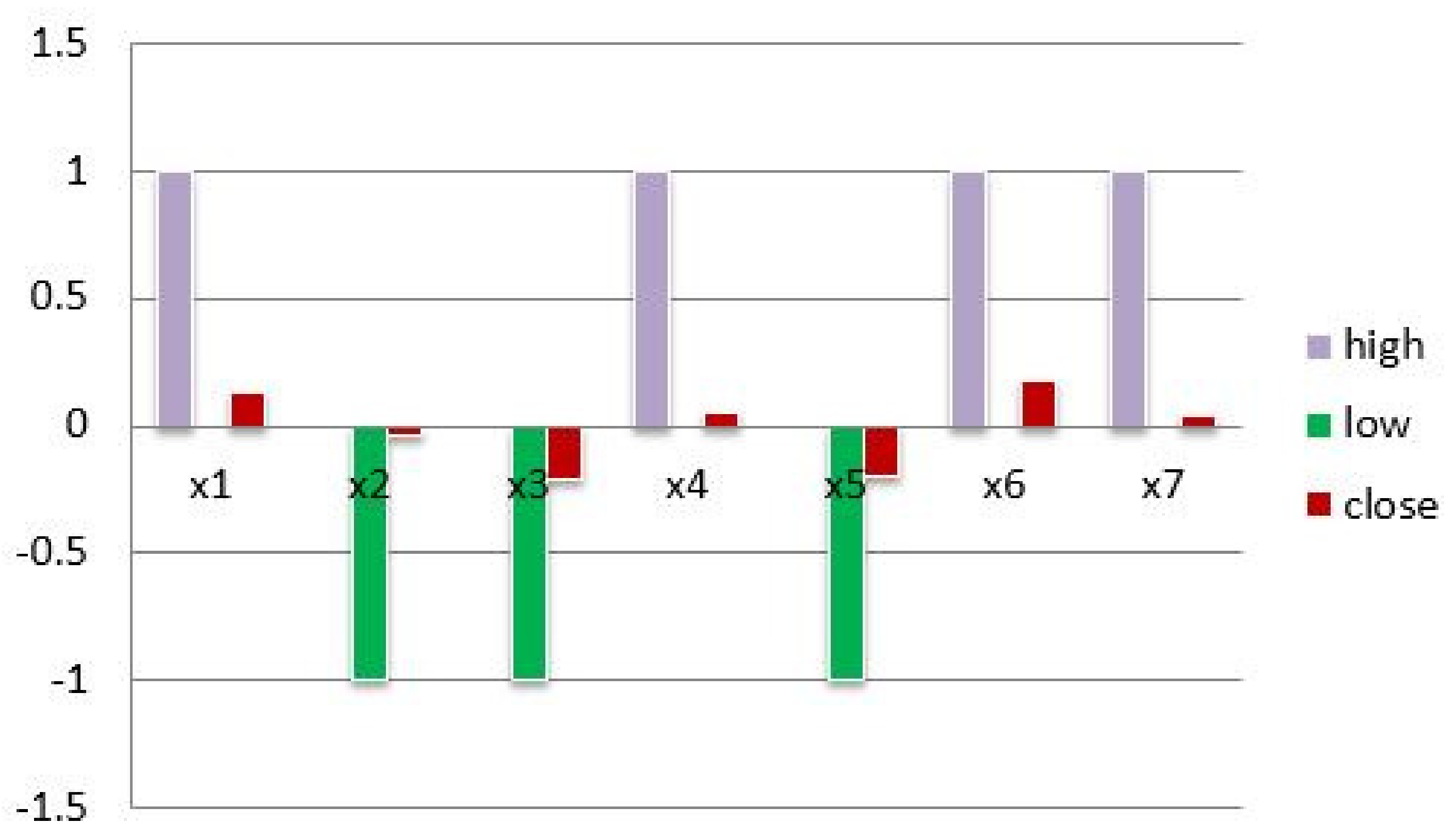
The score function values of alternatives are given in

Table 4. Score function values of alternatives.

X	$\mathit{S}={\mathit{\mu }}^2-{\mathit{\eta }}^2$	Ranking
$x_1$	$0.1322$	2
$x_2$	$-0.0436$	7
$x_3$	$-0.2080$	6
$x_4$	$0.0548$	3
$x_5$	$-0.2010$	5
$x_6$	$0.1749$	1
$x_7$	$0.0367$	4

and the ranking of companies/alternatives is shown in Figure 2.

Table 4 demonstrates that ranking of companies is as follows,

$$x_6\succ x_1\succ x_4\succ x_7\succ x_5\succ x_3\succ x_2.$$

The ranking of companies is also shown in the Figure 2.

Hence, the firm should invest $45\%$ of the capital on $x_6$, $25\%$ on $x_1$, $20\%$ on $x_4$ and the rest $10\%$ on $x_7$.

6. AHP-TOPSIS Approach for Environmental Mitigation with SFS-Topology

This section examines the use of SFSS-topology in multi-criteria group decision making (MCGDM). Following the AHP-TOPSIS extension to SFSSs, we will explore how to save the environment considering the factors polluting the environment and SFSS-topology. AHP- TOPSIS is one of the most-often-used strategies in solving such issues. Though, every strategy has advantages and disadvantages, depending on the problem at hand.

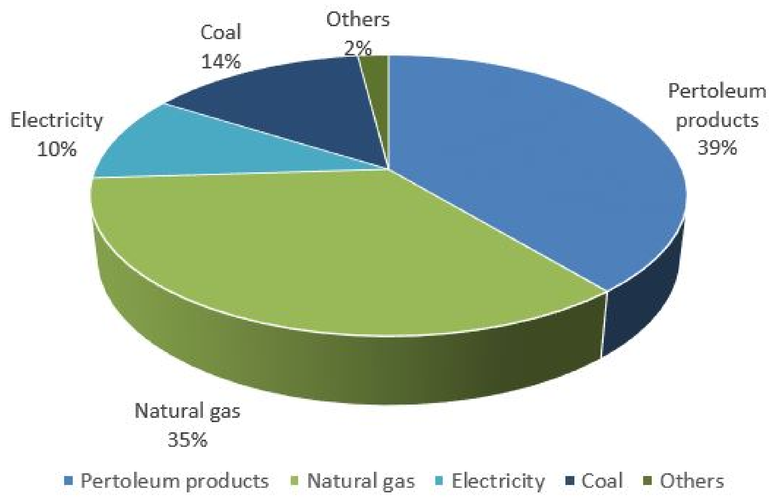
• Case study
  Environmental degradation in Pakistan comprises air quality, water contamination, traffic noise, global warming, chemical abuse, desertification, natural catastrophes, dunes, and storms. A worldwide environmental-performance index (EPI) has previously labelled Pakistan’s air quality as deplorable. Global warming poses a serious threat to the lives of the citizens in the state. Emissions of greenhouse gases, increasing urbanization, and deforestation all play a role in the current state of affairs. Climate change is running amok in low-income countries such as Pakistan. It is not alone in being helpless, as advanced economies—most notably China and the United States—postpone lowering emissions. Global warming will have a significant impact on Pakistan, as well as the Maldives and many other island nations. In contrast to many other countries that have addressed the issue of global emissions at the UN, Pakistan is doing little to safeguard its future. Regular agricultural cycles have helped Pakistan’s economy weather several crises. However, if the IPCC Article is accurate, the country will be underwater by 2050. Already, Pakistan is struggling with a slew of environmental challenges. Many lives have been lost due to weather extremes, which also have a major impact on crop cycles and harvests. Floods decimated Pakistan’s two main cities this year: Karachi and Islamabad. Due to landslides, Pakistan’s commercial lifeline with China, the 806-kilometer Karakoram Highway, was shut down many times for multiple days. There was considerable deforestation in the northern part of Kohistan and the southern part of Jaglot, which led to the deadly landslides. The logging mafias are swiftly clearing old-growth forests north of Shimshal and east of the Skardu Valley, virtually insuring future environmental catastrophes. The state government appears utterly unconcerned about the looming crisis. Not much effort has been put towards meeting its goal of producing 60% of its power from renewable sources by 2030. More than 60% of the country’s electricity is generated from fossil fuels at the moment. Figure 3 shows the key environmental issues in Pakistan.
• Economic ramifications of environmental devastation
  Agriculture and fishing employ more than two-thirds of the workforce in Pakistan and produce over a quarter of the country’s total output. Increased use of finite natural resources is necessary for economic growth. Oddly, the very thing that is enabling this country to develop also constitutes a danger to its long-term safety and stability. A total of 70 percent of Pakistan’s population lives in rural areas and suffers from high poverty levels, according to the World Bank. To make money, these people rely on utilization and conservation, which they tend to misuse. This leads to greater ecological damage, which in turn, enhances impoverishment. This has culminated in a “vicious downward spiral of impoverishment and environmental degradation,” as stated by the World Bank. Pollution-related wellness factors influence both urban and rural dwellers, as per a 2013 World Bank evaluation. Air quality is the state’s most critical environmental challenge. Not only do these global impacts harm Pakistanis, but they often put the country’s business in jeopardy. In the article, growing industrialization, globalization, and vehicular use are anticipated to aggravate the situation.
• Water pollution
  Pakistan is rated as a water-stressed country by the World Economic forum. The Kabul River flows from Afghanistan into Pakistan; whereas the Indus, Jhelum, Chenab, Ravi, and Sutlej Rivers flow from India into Pakistan. Under the Indus Waters Treaty of 1960, water from the Ravi and Sutlej waters is redirected upstream to India for household consumption. The Indus (main stem), Jhelum, and Chenab rivers supply water to the agricultural lands of Punjab and Sindh, though not to the remainder of the region. Pakistan’s economy and the welfare of millions of Pakistanis are strongly effected by resource depletion. With the Law of the Sea Convention and canal diversion, Pakistan’s rivers have fewer diluting flows. The size of the economy, as well as a lack of water treatment, have caused a spike in water pollution. To provide water to people, dumped raw sewage is drained into rivers and the ocean, and unsanitary pipes are used. Water contamination makes it increasingly challenging to acquire safe drinking water and elevates the likelihood of developing an illness carried through raw sewage. There are many ailments that may be largely attributed to filthy water in Pakistan, because of this. Indeed, 45 percent of infant deaths and 60 percent of aquatic infections are caused by diarrhoea.
• Noise pollution
  Some of Pakistan’s urbanized areas are plagued by a substantial amount of noise pollution. Noise pollution is generally triggered by traffic, including vehicles, automobiles, lorries, wheelers, and water tankers. An analysis found that Karachi’s main route seemed to have an average noise level of 90 dB and may reach as high as 110 dB. As a matter of fact, this surpasses the 70 dB limit set by the “International Organization for Standardization (ISO)”. According to the studies, the Environmental Quality Agency’s ambient noise standard in Pakistan is 85 decibels (dB). This threshold of noise pollution might have an influence on both auditory and quasi abilities. There seems to be a diversity of non-auditory clinical depression, notably insomnia, hearing and myocardial sickness, neuroendocrine sensitivity to loudness, and mental disorders. There are only a few, inconsistent noise regulations and policies in place. There is no culpability and the municipal and regional environmental conservation agencies are unable to intervene due to various statutory limitations and a loss of specific norms and regulations, which hinders them from doing so.
• Air pollution
  Wellbeing has been shown to be disproportionately affected by air pollution. For Pakistanis who habitually inhale dirty air, nanoparticle matter variations are a big concern. Respiratory difficulties have been associated to SPM in Pakistan’s largest cities, according to the research. Sustainable fuels such as liquefied petroleum gas (LPG) and improved transportation construction and sustainability can significantly minimize urban air pollution in Pakistan. The government can also adopt mitigation policies to reduce emissions. Pollution levels are increasing in Pakistan’s metro areas. Karachi’s urban air pollution is one of the worst in the world, having a devastating impact on both human development and health. Unsustainable energy use combined with the increased utilisation of automobiles, unauthorized corporate emissions, and debris and polymer combustion have all contributed to urban air pollution. According to the Sindh Environmental Conservation Department, urban air quality is approximately four times that proposed by the World Health Organization. These contaminants contribute to “respiratory disorders, impaired vision, vegetation degradation, and crop production”. Economic production leads to air pollution. An unavoidable byproduct and insufficient air pollution legislation have led to cities’ poor air quality. Abid Omar founded the Pakistan ambient air initiative in 2018, to evaluate the country’s major cities’ air quality. In Pakistan, the US State Department has established three elevated air-quality monitoring units. To overcome such environmental issues, various aspects should be taken under view and numerous efforts are required in order to obtain environmentally friendly conditions. Some are listed below:
  • The establishment of a large tree plantation.
  • Going paperless has the potential to significantly reduce the rate of deforestation on Earth.
  • The number of diesel-powered automobiles that pollute the atmosphere should be reduced.
  • An effective system for treating and managing sewage should be put in place.
  • The practice of living a water-conserving lifestyle should be encouraged.
  One of the most crucial objectives is to achieve an appropriate and effective level of environmental remediation and protection. Policymakers and decision makers must acknowledge that a sustainable plan for solving global crises must be a consistent effort comes from a long approach that combines all stakeholders. Inevitably, the project’s performance is determined by organizational commitment and dedication at every phase of the process, in addition to endorsement of adequate systems and guidelines at all levels. A method to tackle the ecological disaster has several merits, some of which are listed below.
  • Recovering a susceptible and priceless expedient.
  • Increasing the efficacy of currently available systems.
  • Exploiting infrastructure’s massive financial assets.
  • Extending the systems’ average life duration.
  • Increasing revenue from environmental mitigation services.
  • Energy-demand reduction.
  • Decrease in the service’s carbon footprint.
  In order to locate and accentuate the finest solution to environmental issues, a thorough structure of tactics is developed in this study. To be sustainable, the plan chosen must be in harmony with the ecological sector’s integrated approach. Rather than a laborious process of making recommendations that account for the fact that many particular objectives and opportunities exist in the market, a well-organized approach that can be articulated promptly and succinctly must account for concerns of various individuals and those of the constitutionally sound authorities. Decisions are being made by legislators and selection analysts who are well-versed in the process. A review of the literature on environmental strategic planning undertaken with professionals and authorities, as well as information concerning the region of convenience’s domestic life, resulted in the improvement of these measures. Climate-remediation approaches were applied in the environmental distribution network. When a long-term ecological safeguard system exists, clear provisions are often in place. Appraisal attributes are used to assess the effectiveness of each methodology. To choose the optimal method, first, the critical nature of grading parameters should be understood. Attributes are given in

  Table 5. Strategies for environmental mitigation.

  Code	Strategies
  $A_1$	Forest conservation
  $A_2$	Disaster mitigation
  $A_3$	Environmental legislation
  $A_4$	Eliminate the use of fossil-fuel vehicles
  $A_5$	Eliminate single-use plastics
  $A_6$	Agriculture that is sustainable
  $A_7$	Mitigation of environmental aspects of aviation

  as the strategies to overcome environmental crises, and judgement criteria are given in

  Table 6. Explanation of the evaluation criteria.

  Code	Strategies	Explanation
  ${\acute{C}}_1$	Cost figure	Expenditure associated with the implementation of the criteria
  ${\acute{C}}_2$	Benefit period	Calculation of the effective life span of the criteria
  ${\acute{C}}_3$	Energy Saved	For a solution to be viable, it must be able to cut energy consumption and global-warming emissions.
  ${\acute{C}}_4$	Supply reliability	The criteria may be preferable if it is capable of saving a long-term service and easing supply constraints.
  ${\acute{C}}_5$	Flexibility	The criteria should be tailored to meet diverse needs and uncertainties in order to be more flexible.
  ${\acute{C}}_6$	Social acceptance	If the criteria has ability to be accepted by the localities.

  .
  The linguistic terms for judging alternatives are listed in

  Table 7. Linguistic terms for judging alternatives.

  Linguistic Terms	Score Index
  Equal importance (EI)	1
  Moderate importance (MI)	3
  Strong important (SI)	5
  Very-strong importance (VI)	7
  Extreme importance (EXI)	9

  .

Note that:

• Intermediate values for two consecutive linguistic terms will be $\left(I{V}_1\right),\left(I{V}_2\right),\left(I{V}_3\right),$$\left(I{V}_4\right)$ as 2, 4, 6, 8, respectively
• Values for inverse composition for each linguistic term will be the reciprocal of its score index.

Algorithm 2 AHP-TOPSIS.

Step 1. Consider $D=\{D_i:i=1,2,···,l\}$ as a set of decision makers, $A=\{A_j:j=1,2,···,m\}$ as a set of alternatives and $C=\{{\acute{C}}_k:j=1,2,···,n\}$ as a set of parameters/criterion. Step 2. By selecting the linguistic terms from Table 7, pair-wise comparison matrix is constructed as $${\left[W_{ij}\right]}_{n\times m}=\left(\begin{array}{cccc}{W}_{11}& W_{12}& \cdots & W_{1m}\\ W_{21}& W_{22}& \cdots & W_{2m}\\ ⋮& ⋮& \ddots & ⋮\\ W_{i1}& W_{i2}& \cdots & W_{im}\\ ⋮& ⋮& \ddots & ⋮\\ W_{n1}& W_{n2}& \cdots & W_{nm}\end{array}\right)$$ where $W_{ij}$ is the values assigned by the experts $D_i$ to the alternative $A_j$ by considering linguistic terms as given in Table 7. Step 3. Compute normalized pair-wise comparison matrix $${\left[{\widehat{\varrho }}_{ij}\right]}_{n\times m}=\left(\begin{array}{cccc}{\widehat{\varrho }}_{11}& {\widehat{\varrho }}_{12}& \cdots & {\widehat{\varrho }}_{1m}\\ {\widehat{\varrho }}_{21}& {\widehat{\varrho }}_{22}& \cdots & {\widehat{\varrho }}_{2m}\\ ⋮& ⋮& \ddots & ⋮\\ {\widehat{\varrho }}_{i1}& {\widehat{\varrho }}_{i2}& \cdots & {\widehat{\varrho }}_{im}\\ ⋮& ⋮& \ddots & ⋮\\ {\widehat{\varrho }}_{n1}& {\widehat{\varrho }}_{n2}& \cdots & {\widehat{\varrho }}_{nm}\end{array}\right)$$ where ${\widehat{\varrho }}_{ij}=\frac{W_{ij}}{{\Sigma }_{i=1}^m{W}_{ij}}$. Step 4. Obtain the weighted vector $\mathcal{W}=(w_1,w_2,\cdots ,w_m)$ where $w_i=\frac{{\Sigma }_{j=1}^m{\widehat{\varrho }}_{ij}}{m}$. Step 5. Calculate the consistency to check whether the calculated values are correct or not. For this purpose, follow the steps given below i.  Take the pair-wise comparison matrix from Step 2. ii.  Multiply this matrix by the weight vector $\mathcal{W}=(w_1,w_2,\cdots ,w_m)$, such as $P_{ij}=W_{ij}\times w_j$ for $j=1,2,\cdots ,m.$ iii.  Now, calculate eigen values ${\lambda }_i$, for $i=1,2,\cdots ,m$ given that ${\lambda }_i=\frac{{\sum }_{j=1}^m{P}_{ij}}{w_i}.$ iv.  Obtain the value of ${\lambda }_{max}$ using, ${\lambda }_{max}=\frac{{\sum }_{i=1}^m{\lambda }_i}{m}.$ v.  Calculate the value of the consistency index (CI), such that $\mathit{CI}=\frac{{\lambda }_{max}-m}{m-1}$ where, m is the number of compared elements. vi.  Obtain the value of consistency ratio (CR), utilizing $\mathit{CR}=\frac{\mathit{CI}}{\mathit{RI}}$ where, random index (RI) is the consistency index of the randomly generated pair-wise matrix. vii.  Check whether CR follows the inequality, $\mathit{CR}<0.10$. If yes, then the weights are consistent. Otherwise, use different linguistic scores in Step 2. Step 6. Write the SFSS decision matrix $$D_i={\left[v_{jk}^i\right]}_{m\times n}=\left(\begin{array}{ccccc}& {\acute{C}}_1& {\acute{C}}_2& \cdots & {\acute{C}}_n\\ A_1& v_{11}^i& v_{12}^i& \cdots & v_{1n}^i\\ A_2& v_{21}^i& v_{22}^i& \cdots & v_{2n}^i\\ & ⋮& ⋮& \ddots & ⋮\\ A_j& v_{j1}^i& v_{j2}^i& \cdots & v_{jn}^i\\ & ⋮& ⋮& \ddots & ⋮\\ A_m& v_{m1}^i& v_{m2}^i& \cdots & v_{mn}^i\end{array}\right)$$ where $v_{jk}^i$ is the SFSS-element of $i$th decision maker to $j$th alternative under $k$th criteria, such that $D_i$$(i=1,2,···,l)$ makes an SFSS-topolgy. Then, we obtain the aggregating matrix using $$\frac{D_1+D_2+\cdots +D_l}{l}={\left[{\dot{v}}_{jk}\right]}_{m\times n}$$ Step 7. Obtain the weighted SFSS decision matrix $${\left[{\ddot{v}}_{jk}\right]}_{m\times n}=\left(\begin{array}{cccc}{\ddot{v}}_{11}& {\ddot{v}}_{12}& \cdots & {\ddot{v}}_{1n}\\ {\ddot{v}}_{21}& {\ddot{v}}_{22}& \cdots & {\ddot{v}}_{2n}\\ ⋮& ⋮& \ddots & ⋮\\ {\ddot{v}}_{j1}& {\ddot{v}}_{j2}& \cdots & {\ddot{v}}_{jn}\\ ⋮& ⋮& \ddots & ⋮\\ {\ddot{v}}_{m1}& {\ddot{v}}_{m2}& \cdots & {\ddot{v}}_{mn}\end{array}\right)$$ where ${\ddot{v}}_{jk}=w_k\times {\dot{v}}_{jk}$. Step 8. In order to obtain the SFSS-valued positive ideal solution (SFSV-PIS) and SFSS-valued negative ideal solution (SFSV-NIS), we employ, in order, $$\begin{array}{lll}SFSV-PIS\hfill & =& \{{\ddot{v}}_1^{+},{\ddot{v}}_2^{+},\cdots ,{\ddot{v}}_m^{+}\}\hfill \\ & =& \left\{\left({\vee }_j{\ddot{v}}_{jk}\right)\right\}\end{array}$$ where, $${\vee }_j{\ddot{v}}_{jk}=\left\{(max\left\{{\mu }_{jk}\left(x\right)\right\},min\left\{{\gamma }_{jk}\left(x\right)\right\},min\left\{{\eta }_{jk}\left(x\right)\right\})\right|x\in X\}$$ and $$\begin{array}{lll}SFSV-NIS\hfill & =& \{{\ddot{v}}_1^{-},{\ddot{v}}_2^{-},\cdots ,{\ddot{v}}_m^{-}\}\hfill \\ & =& \left\{({\wedge }_j{\ddot{v}}_{jk}\right\}\end{array}$$ where, $${\wedge }_j{\ddot{v}}_{jk}=\left\{(min\left\{{\mu }_{jk}\left(x\right)\right\},max\left\{{\gamma }_{jk}\left(x\right)\right\},max\left\{{\eta }_{jk}\left(x\right)\right\})\right|x\in X\}$$ Step 9. SFSS–Euclidean distances of each alternative from SFSV-PIS and SFSV-NIS, respectively, are computed as; $$d_j^{+}=\sqrt{{\Sigma }_{k=1}^m\left\{{\left({\mu }_{jk}-{\mu }_k^{+}\right)}^2+{\left({\gamma }_{jk}-{\gamma }_k^{+}\right)}^2+{\left({\eta }_{jk}-{\eta }_k^{+}\right)}^2\right\}}$$ and $$d_j^{-}=\sqrt{{\Sigma }_{k=1}^m\left\{{\left({\mu }_{jk}-{\mu }_k^{-}\right)}^2+{\left({\gamma }_{jk}-{\gamma }_k^{-}\right)}^2+{\left({\eta }_{jk}-{\eta }_k^{-}\right)}^2\right\}}$$ Step 10. Calculate the coefficient of closeness amongst each alternative and the ideal solution, using $$C_j^{-}\left({\ddot{v}}_j\right)=\frac{d_j^{-}}{d_j^{+}+d_j^{-}}\in [0,1]$$ Step 11. We can determine the preferred choices by putting them into decreasing (or increasing) order.

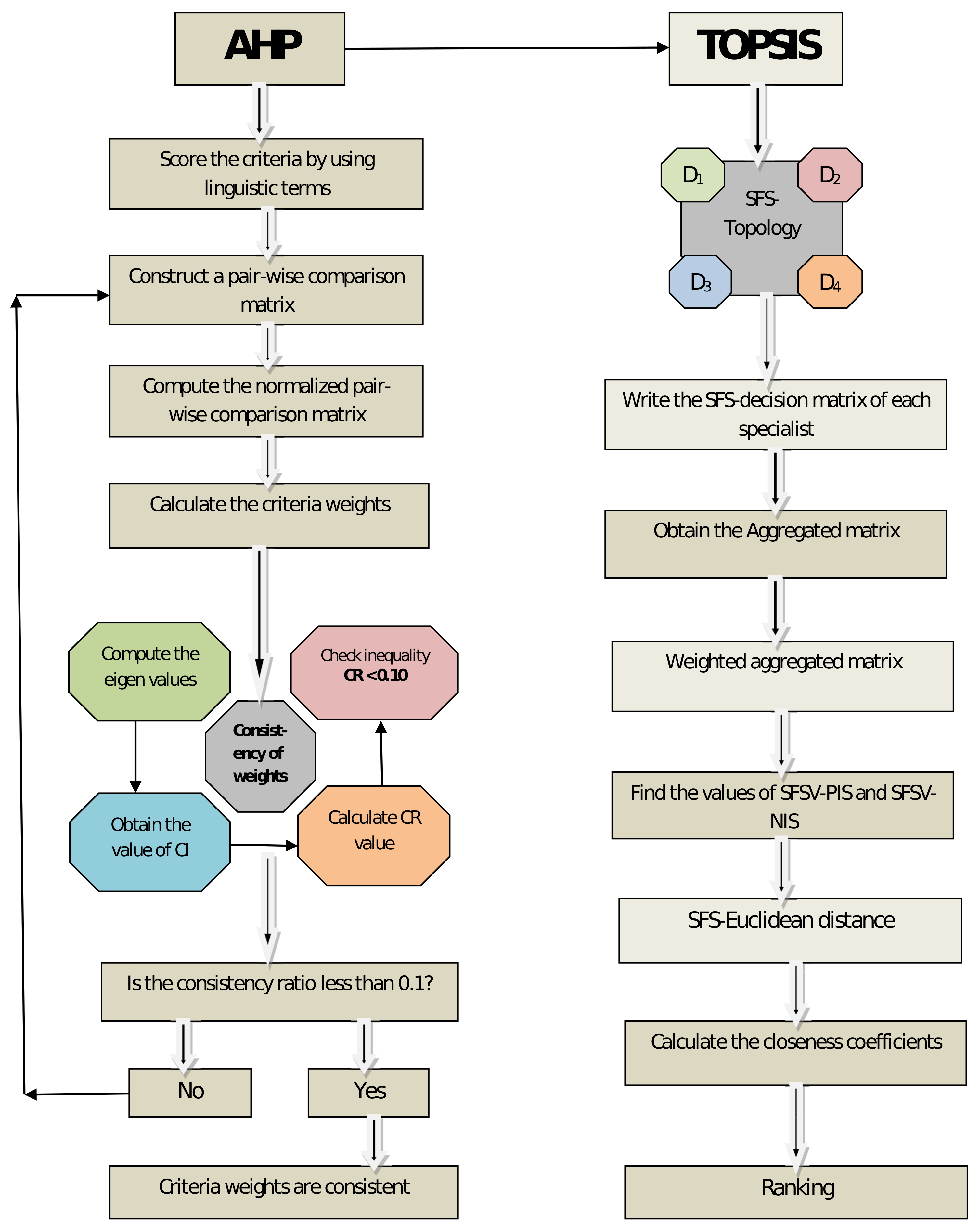
The flow chart of AHP-TOPSIS for SFSS information is given in Figure 4.

Example 17.

As an illustration of Algorithm 2, the demonstrative example for environmental mitigation strategies is presented.

Step 1

Let $A=\{A_1,···,A_7\}$ be the collection of alternatives and $C=\{{\acute{C}}_1,···,{\acute{C}}_6\}$ be the collection of evaluation criteria as given in Table 3 and Table 4, respectively. We will use the set $D=\{D_1,···,D_4\}$ to refer to a group of policymakers / decision makers who have been asked to score each approach on the basis of how well it meets each of the evaluation criteria in terms of SFNs.

Step 2

We determined the relative importance of each criteria with respect to our goal in

Table 8. Relative importance of criteria.

	${\acute{\mathit{C}}}_1$	${\acute{\mathit{C}}}_2$	${\acute{\mathit{C}}}_3$	${\acute{\mathit{C}}}_4$	${\acute{\mathit{C}}}_4$	${\acute{\mathit{C}}}_6$
${\acute{C}}_1$	$EI$	$I{V}_2$	$VI$	$MI$	$SI$	$I{V}_1$
${\acute{C}}_2$	$I{V}_2$	$EI$	$I{V}_1$	$VI$	$I{V}_2$	$SI$
${\acute{C}}_3$	$VI$	$I{V}_1$	$EI$	$MI$	$I{V}_3$	$EXI$
${\acute{C}}_4$	$MI$	$VI$	$MI$	$EI$	$SI$	$VI$
${\acute{C}}_5$	$SI$	$I{V}_2$	$I{V}_2$	$SI$	$EI$	$I{V}_2$
${\acute{C}}_6$	$I{V}_1$	$SI$	$EXI$	$VI$	$I{V}_2$	$EI$

. Whereas, in

Table 9. Pair-wise comparison matrix.

	${\acute{\mathit{C}}}_1$	${\acute{\mathit{C}}}_2$	${\acute{\mathit{C}}}_3$	${\acute{\mathit{C}}}_4$	${\acute{\mathit{C}}}_4$	${\acute{\mathit{C}}}_6$
${\acute{C}}_1$	$1.000$	$4.000$	$7.000$	$3.000$	$5.000$	$2.000$
${\acute{C}}_2$	$0.250$	$1.000$	$0.500$	$7.000$	$4.000$	$5.000$
${\acute{C}}_3$	$0.143$	$2.000$	$1.000$	$3.000$	$6.000$	$9.000$
${\acute{C}}_4$	$0.333$	$0.143$	$0.333$	$1.000$	$5.000$	$0.143$
${\acute{C}}_5$	$0.200$	$0.250$	$0.167$	$0.200$	$1.000$	$4.000$
${\acute{C}}_6$	$0.500$	$0.200$	$0.111$	$7.000$	$0.250$	$1.000$

, a pair-wise comparison matrix is created with the help of the linguistic terms from Table 7.

Step 3

Then, we obtained normalized pair-wise comparison matrix, which is given in

Table 10. Normalized pair-wise comparison matrix.

	${\acute{\mathit{C}}}_1$	${\acute{\mathit{C}}}_2$	${\acute{\mathit{C}}}_3$	${\acute{\mathit{C}}}_4$	${\acute{\mathit{C}}}_4$	${\acute{\mathit{C}}}_6$
${\acute{C}}_1$	$0.243$	$0.527$	$0.768$	$0.142$	$0.235$	$0.095$
${\acute{C}}_2$	$0.061$	$0.132$	$0.055$	$0.330$	$0.188$	$0.236$
${\acute{C}}_3$	$0.035$	$0.263$	$0.110$	$0.142$	$0.282$	$0.426$
${\acute{C}}_4$	$0.081$	$0.019$	$0.037$	$0.047$	$0.235$	$0.007$
${\acute{C}}_5$	$0.049$	$0.033$	$0.018$	$0.009$	$0.047$	$0.189$
${\acute{C}}_6$	$0.122$	$0.026$	$0.012$	$0.330$	$0.012$	$0.047$

.

Step 4

Therefore, the required criteria weights are calculated, as shown in

Table 11. Criteria weights.

${\acute{C}}_1$	$0.335$
${\acute{C}}_2$	$0.167$
${\acute{C}}_3$	$0.210$
${\acute{C}}_4$	$0.071$
${\acute{C}}_5$	$0.058$
${\acute{C}}_6$	$0.092$

.

Step 5

Criteria weights are consistent, as they fulfil the requirement that $CR<0.10$.

Step 6

The evaluations of decision makers in terms of decision matrices $D_1$, $D_2$, $D_3$, and $D_4$ are expressed in

Table 12. Decision matrix $D_1$.

	${\acute{\mathit{C}}}_1$	${\acute{\mathit{C}}}_2$	${\acute{\mathit{C}}}_3$	${\acute{\mathit{C}}}_4$	${\acute{\mathit{C}}}_4$	${\acute{\mathit{C}}}_6$
$A_1$	$(0.82,0.03,0.21)$	$(0.19,0.35,0.28)$	$(0.79,0.16,0.31)$	$(0.68,0.21,0.40)$	$(0.24,0.39,0.41)$	$(0.65,0.13,0.37)$
$A_2$	$(0.16,0.07,0.78)$	$(0.41,0.23,0.56)$	$(0.34,0.19,0.59)$	$(0.42,0.32,0.38)$	$(0.65,0.17,0.39)$	$(0.47,0.21,0.51)$
$A_3$	$(0.52,0.28,0.37)$	$(0.45,0.31,0.36)$	$(0.17,0.38,0.41)$	$(0.34,0.47,0.29)$	$(0.46,0.11,0.52)$	$(0.62,0.18,0.25)$
$A_4$	$(0.47,0.32,0.38)$	$(0.27,0.47,0.38)$	$(0.80,0.04,0.36)$	$(0.35,0.41,0.28)$	$(0.71,0.13,0.29)$	$(0.56,0.29,0.34)$
$A_5$	$(0.73,0.18,0.26)$	$(0.19,0.37,0.49)$	$(0.47,0.21,0.52)$	$(0.61,0.24,0.38)$	$(0.52,0.32,0.47)$	$(0.43,0.24,0.26)$
$A_6$	$(0.43,0.21,0.35)$	$(0.27,0.36,0.53)$	$(0.61,0.28,0.31)$	$(0.71,0.09,0.25)$	$(0.15,0.39,0.53)$	$(0.67,0.21,0.19)$
$A_7$	$(0.83,0.04,0.19)$	$(0.38,0.27,0.57)$	$(0.46,0.19,0.52)$	$(0.75,0.18,0.26)$	$(0.59,0.28,0.37)$	$(0.37,0.28,0.49)$

,

Table 13. Decision matrix $D_2$.

	${\acute{\mathit{C}}}_1$	${\acute{\mathit{C}}}_2$	${\acute{\mathit{C}}}_3$	${\acute{\mathit{C}}}_4$	${\acute{\mathit{C}}}_4$	${\acute{\mathit{C}}}_6$
$A_1$	$(0.00,0.00,1.00)$	$(0.00,0.00,1.00)$	$(0.00,0.00,1.00)$	$(0.00,0.00,1.00)$	$(0.00,0.00,1.00)$	$(0.00,0.00,1.00)$
$A_2$	$(0.00,0.00,1.00)$	$(0.00,0.00,1.00)$	$(0.00,0.00,1.00)$	$(0.00,0.00,1.00)$	$(0.00,0.00,1.00)$	$(0.00,0.00,1.00)$
$A_3$	$(0.00,0.00,1.00)$	$(0.00,0.00,1.00)$	$(0.00,0.00,1.00)$	$(0.00,0.00,1.00)$	$(0.00,0.00,1.00)$	$(0.00,0.00,1.00)$
$A_4$	$(0.00,0.00,1.00)$	$(0.00,0.00,1.00)$	$(0.00,0.00,1.00)$	$(0.00,0.00,1.00)$	$(0.00,0.00,1.00)$	$(0.00,0.00,1.00)$
$A_5$	$(0.00,0.00,1.00)$	$(0.00,0.00,1.00)$	$(0.00,0.00,1.00)$	$(0.00,0.00,1.00)$	$(0.00,0.00,1.00)$	$(0.00,0.00,1.00)$
$A_6$	$(0.00,0.00,1.00)$	$(0.00,0.00,1.00)$	$(0.00,0.00,1.00)$	$(0.00,0.00,1.00)$	$(0.00,0.00,1.00)$	$(0.00,0.00,1.00)$
$A_7$	$(0.00,0.00,1.00)$	$(0.00,0.00,1.00)$	$(0.00,0.00,1.00)$	$(0.00,0.00,1.00)$	$(0.00,0.00,1.00)$	$(0.00,0.00,1.00)$

,

Table 14. Decision matrix $D_3$.

	${\acute{\mathit{C}}}_1$	${\acute{\mathit{C}}}_2$	${\acute{\mathit{C}}}_3$	${\acute{\mathit{C}}}_4$	${\acute{\mathit{C}}}_4$	${\acute{\mathit{C}}}_6$
$A_1$	$(0.62,0.21,0.38)$	$(0.39,0.41,0.28)$	$(0.84,0.07,0.19)$	$(0.19,0.37,0.64)$	$(0.48,0.25,0.53)$	$(0.23,0.48,0.51)$
$A_2$	$(0.70,0.18,0.27)$	$(0.53,0.24,0.36)$	$(0.63,0.15,0.31)$	$(0.34,0.28,0.59)$	$(0.61,0.14,0.32)$	$(0.63,0.17,0.28)$
$A_3$	$(0.53,0.23,0.46)$	$(0.19,0.46,0.51)$	$(0.47,0.32,0.35)$	$(0.56,0.19,0.43)$	$(0.37,0.41,0.46)$	$(0.46,0.21,0.43)$
$A_4$	$(0.43,0.26,0.37)$	$(0.25,0.31,0.42)$	$(0.76,0.25,0.24)$	$(0.28,0.39,0.51)$	$(0.21,0.42,0.38)$	$(0.18,0.36,0.59)$
$A_5$	$(0.35,0.29,0.44)$	$(0.46,0.39,0.49)$	$(0.39,0.17,0.61)$	$(0.51,0.08,0.48)$	$(0.75,0.19,0.10)$	$(0.31,0.27,0.48)$
$A_6$	$(0.15,0.37,0.72)$	$(0.23,0.41,0.53)$	$(0.59,0.14,0.47)$	$(0.61,0.04,0.39)$	$(0.52,0.28,0.39)$	$(0.79,0.05,0.20)$
$A_7$	$(0.54,0.16,0.61)$	$(0.17,0.49,0.35)$	$(0.52,0.27,0.41)$	$(0.62,0.19,0.40)$	$(0.81,0.16,0.19)$	$(0.59,0.26,0.38)$

, and

Table 15. Decision matrix $D_4$.

	${\acute{\mathit{C}}}_1$	${\acute{\mathit{C}}}_2$	${\acute{\mathit{C}}}_3$	${\acute{\mathit{C}}}_4$	${\acute{\mathit{C}}}_4$	${\acute{\mathit{C}}}_6$
$A_1$	$(1.00,0.00,0.00)$	$(1.00,0.00,0.00)$	$(1.00,0.00,0.00)$	$(1.00,0.00,0.00)$	$(1.00,0.00,0.00)$	$(1.00,0.00,0.00)$
$A_2$	$(1.00,0.00,0.00)$	$(1.00,0.00,0.00)$	$(1.00,0.00,0.00)$	$(1.00,0.00,0.00)$	$(1.00,0.00,0.00)$	$(1.00,0.00,0.00)$
$A_3$	$(1.00,0.00,0.00)$	$(1.00,0.00,0.00)$	$(1.00,0.00,0.00)$	$(1.00,0.00,0.00)$	$(1.00,0.00,0.00)$	$(1.00,0.00,0.00)$
$A_4$	$(1.00,0.00,0.00)$	$(1.00,0.00,0.00)$	$(1.00,0.00,0.00)$	$(1.00,0.00,0.00)$	$(1.00,0.00,0.00)$	$(1.00,0.00,0.00)$
$A_5$	$(1.00,0.00,0.00)$	$(1.00,0.00,0.00)$	$(1.00,0.00,0.00)$	$(1.00,0.00,0.00)$	$(1.00,0.00,0.00)$	$(1.00,0.00,0.00)$
$A_6$	$(1.00,0.00,0.00)$	$(1.00,0.00,0.00)$	$(1.00,0.00,0.00)$	$(1.00,0.00,0.00)$	$(1.00,0.00,0.00)$	$(1.00,0.00,0.00)$
$A_7$	$(1.00,0.00,0.00)$	$(1.00,0.00,0.00)$	$(1.00,0.00,0.00)$	$(1.00,0.00,0.00)$	$(1.00,0.00,0.00)$	$(1.00,0.00,0.00)$

, respectively. The rows represent the alternatives and the columns represent the parameters in these matrices. Then, the collection of decision matrices forms an SFSS-topology.

As a result, we arrive at an aggregated decision matrix that looks like

Table 16. Aggregated decision matrix.

	${\acute{\mathit{C}}}_1$	${\acute{\mathit{C}}}_2$	${\acute{\mathit{C}}}_3$	${\acute{\mathit{C}}}_4$	${\acute{\mathit{C}}}_4$	${\acute{\mathit{C}}}_6$
$A_1$	$(0.6100,0.0600,0.3975)$	$(0.3950,0.1900,0.3900)$	$(0.6575,0.0575,0.3750)$	$(0.4675,0.1450,0.5100)$	$(0.4300,0.1600,0.4850)$	$(0.4700,0.305,0.4700)$
$A_2$	$(0.4650,0.0625,0.5125)$	$(0.4850,0.1175,0.4800)$	$(0.4925,0.0850,0.4750)$	$(0.4400,0.1500,0.4925)$	$(0.5650,0.0775,0.4275)$	$(0.5250,0.0950,0.4475)$
$A_3$	$(0.5125,0.1275,0.4575)$	$(0.4100,0.1925,0.4675)$	$(0.4100,0.1750,0.4400)$	$(0.4575,0.1300,0.4950)$	$(0.4575,0.1300,0.4950)$	$(0.5200,0.0975,0.4200)$
$A_4$	$(0.4750,0.1450,0.4375)$	$(0.3800,0.1950,0.4500)$	$(0.6400,0.0725,0.4000)$	$(0.4075,0.2000,0.4475)$	$(0.4800,0.1375,0.4175)$	$(0.4350,0.1625,0.4825)$
$A_5$	$(0.5200,0.1175,0.4250)$	$(0.4125,0.1900,0.4950)$	$(0.4650,0.0950,0.5325)$	$(0.5300,0.0800,0.4650)$	$(0.5675,0.1275,0.3925)$	$(0.4350,0.1275,0.435)$
$A_6$	$(0.3950,0.1450,0.5175)$	$(0.3750,0.1925,0.5150)$	$(0.5500,0.1050,0.4450)$	$(0.5800,0.0325,0.4100)$	$(0.4175,0.1675,0.4800)$	$(0.6150,0.0650,0.3475)$
$A_7$	$(0.5925,0.0500,0.4500)$	$(0.3875,0.1900,0.4800)$	$(0.4950,0.1150,0.4825)$	$(0.5925,0.0925,0.4150)$	$(0.6000,0.1100,0.3900)$	$(0.4900,0.1350,0.4675)$

, computed by using $\frac{D_1+D_2+D_3+D_4}{4}$

Step 7

Then, we calculated the weighted SFSS decision matrix, given in

Table 17. Weighted decision matrix.

	${\acute{\mathit{C}}}_1$	${\acute{\mathit{C}}}_2$	${\acute{\mathit{C}}}_3$	${\acute{\mathit{C}}}_4$	${\acute{\mathit{C}}}_4$	${\acute{\mathit{C}}}_6$
$A_1$	$(0.2044,0.0201,0.1332)$	$(0.0660,0.0317,0.0651)$	$(0.1381,0.0121,0.0788)$	$(0.0332,0.0103,0.0362)$	$(0.0249,0.0093,0.0281)$	$(0.0433,0.0281,0.0432)$
$A_2$	$(0.1558,0.0209,0.1717)$	$(0.4081,0.0196,0.0802)$	$(0.1034,0.0179,0.0998)$	$(0.0312,0.0107,0.0350)$	$(0.0328,0.0045,0.0248)$	$(0.0483,0.0087,0.0412)$
$A_3$	$(0.1717,0.0427,0.1533)$	$(0.0684,0.0321,0.0781)$	$(0.0861,0.0368,0.0924)$	$(0.0325,0.0092,0.0351)$	$(0.0266,0.0075,0.0287)$	$(0.0478,0.0090,0.0386)$
$A_4$	$(0.1591,0.0486,0.1466)$	$(0.0635,0.0326,0.0752)$	$(0.1344,0.0152,0.0840)$	$(0.0289,0.0142,0.0318)$	$(0.0278,0.0080,0.0242)$	$(0.0400,0.0150,0.0444)$
$A_5$	$(0.1742,0.0394,0.1424)$	$(0.0689,0.0317,0.0827)$	$(0.0977,0.0199,0.1118)$	$(0.0376,0.0057,0.0330)$	$(0.0329,0.0074,0.0228)$	$(0.0400,0.0117,0.0400)$
$A_6$	$(0.1323,0.0486,0.1734)$	$(0.0626,0.0321,0.0860)$	$(0.1155,0.0221,0.0935)$	$(0.0412,0.0023,0.0291)$	$(0.0242,0.0097,0.0278)$	$(0.0566,0.0060,0.0319)$
$A_7$	$(0.1984,0.0168,0.1508)$	$(0.0647,0.0317,0.0802)$	$(0.1040,0.0242,0.1013)$	$(0.0421,0.0066,0.0295)$	$(0.0348,0.0064,0.0226)$	$(0.0451,0.0124,0.0430)$

.

Step 8

Then, we obtained the SFSS-valued positive ideal solution (SFSV-PIS) and SFSS-valued negative ideal solution (SFSV-NIS).

$$\begin{gathered} SFSV-PIS=\{{\ddot{\wp }}_1^{+},{\ddot{\wp }}_2^{+},{\ddot{\wp }}_3^{+},{\ddot{\wp }}_4^{+},{\ddot{\wp }}_5^{+},{\ddot{\wp }}_6^{+}\} \\ =\left\{(0.2044,0.0168,0.1332),(0.4081,0.0196,0.0651),(0.1381,0.0121,0.0788), \\ (0.0421,0.0023,0.0291),(0.0348,0.0045,0.0226),(0.0566,0.0060,0.0319)\right\} \end{gathered}$$.

$$\begin{gathered} SFSV-NIS=\{{\ddot{\wp }}_1^{-},{\ddot{\wp }}_2^{-},{\ddot{\wp }}_3^{-},{\ddot{\wp }}_4^{-}{\ddot{\wp }}_5^{-},{\ddot{\wp }}_6^{-}\} \\ =\left\{(0.1323,0.0486,0.1734),(0.0626,0.0326,0.0860),(0.0861,0.0368,0.1118), \\ (0.0289,0.0142,0.0362),(0.0242,0.0097,0.0287),(0.0400,0.0281,0.0444)\right\} \end{gathered}$$.

Step 9

The SFSS-Euclidean distances of each alternative from SFSV-PIS and SFSV-NIS are computed as given in

Table 18. Positive ideal solution.

$d_1^{+}=d^{+}({\ddot{v}}_1,\mathrm{SFSV}\text{-}\mathrm{PIS})$	$0.3440$
$d_2^{+}=d^{+}({\ddot{v}}_2,\mathrm{SFSV}\text{-}\mathrm{PIS})$	$0.0785$
$d_3^{+}=d^{+}({\ddot{v}}_3,\mathrm{SFSV}\text{-}\mathrm{PIS})$	$0.3490$
$d_4^{+}=d^{+}({\ddot{v}}_4,\mathrm{SFSV}\text{-}\mathrm{PIS})$	$0.3510$
$d_5^{+}=d^{+}({\ddot{v}}_5,\mathrm{SFSV}\text{-}\mathrm{PIS})$	$0.3467$
$d_6^{+}=d^{+}({\ddot{v}}_6,\mathrm{SFSV}\text{-}\mathrm{PIS})$	$0.3589$
$d_7^{+}=d^{+}({\ddot{v}}_7,\mathrm{SFSV}\text{-}\mathrm{PIS})$	$0.3475$

and

Table 19. Negative ideal solution.

$d_1^{-}=d^{-}({\ddot{v}}_1,\mathrm{SFSV}\text{-}\mathrm{NIS})$	$0.1119$
$d_2^{-}=d^{-}({\ddot{v}}_2,\mathrm{SFSV}\text{-}\mathrm{NIS})$	$0.3497$
$d_3^{-}=d^{-}({\ddot{v}}_3,\mathrm{SFSV}\text{-}\mathrm{NIS})$	$0.0545$
$d_4^{-}=d^{-}({\ddot{v}}_4,\mathrm{SFSV}\text{-}\mathrm{NIS})$	$0.0725$
$d_5^{-}=d^{-}({\ddot{v}}_5,\mathrm{SFSV}\text{-}\mathrm{NIS})$	$0.0619$
$d_6^{-}=d^{-}({\ddot{v}}_6,\mathrm{SFSV}\text{-}\mathrm{NIS})$	$0.0518$
$d_7^{-}=d^{-}({\ddot{v}}_7,\mathrm{SFSV}\text{-}\mathrm{NIS})$	$0.0850$

, respectively.

Step 10

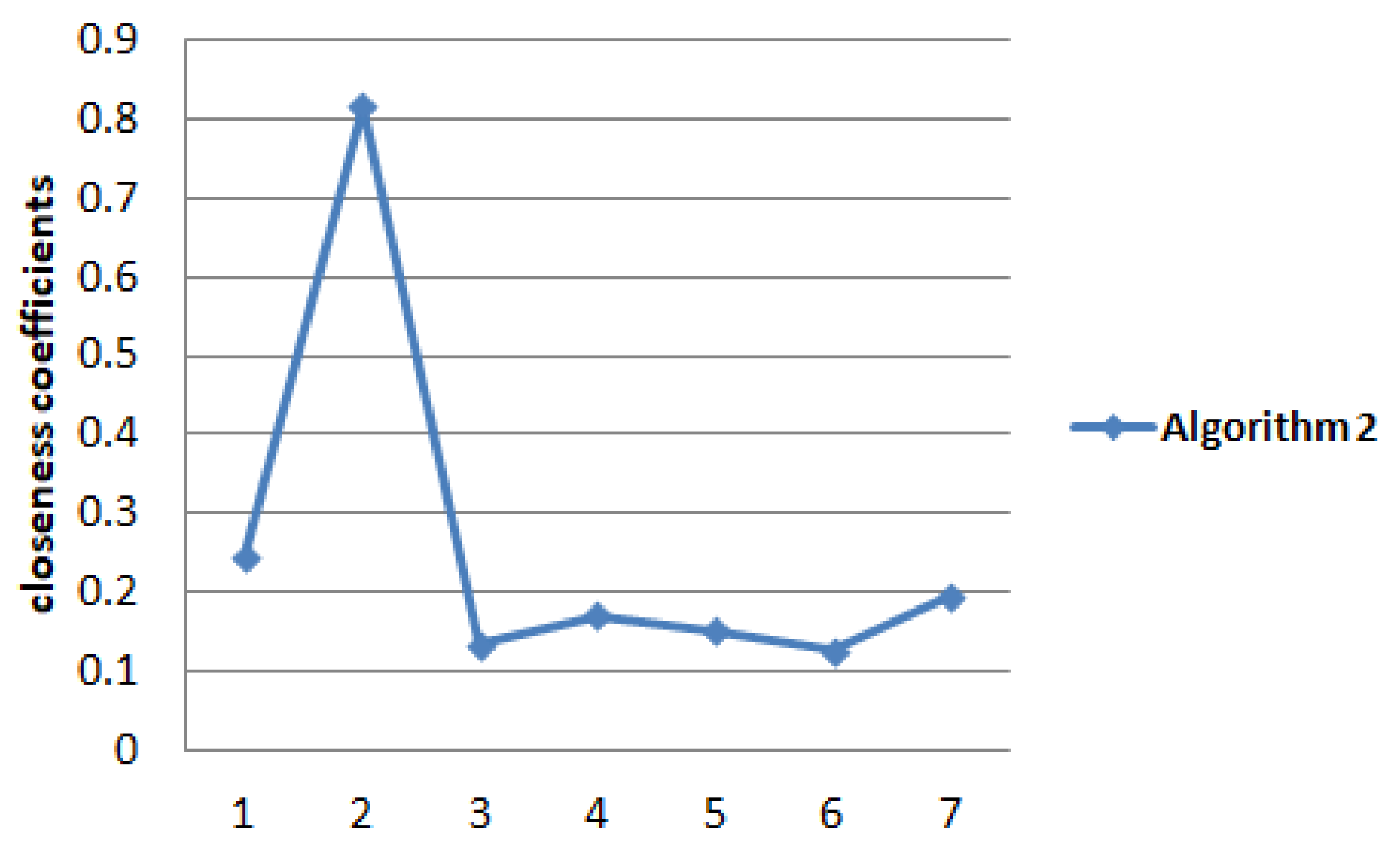
Each alternative was compared to the ideal solution in

Table 20. Closeness coefficient.

$C_1^{-}\left({\ddot{v}}_1\right)$	0.2454
$C_2^{-}\left({\ddot{v}}_2\right)$	0.8167
$C_3^{-}\left({\ddot{v}}_3\right)$	0.1351
$C_4^{-}\left({\ddot{v}}_4\right)$	0.1712
$C_5^{-}\left({\ddot{v}}_5\right)$	0.1515
$C_6^{-}\left({\ddot{v}}_6\right)$	0.1261
$C_7^{-}\left({\ddot{v}}_7\right)$	0.1965

, in order to compute its closeness coefficient.

Step 11

The preference order of the alternatives, therefore, is

$${\ddot{v}}_2\succ {\ddot{v}}_1\succ {\ddot{v}}_7\succ {\ddot{v}}_4\succ {\ddot{v}}_5\succ {\ddot{v}}_3\succ {\ddot{v}}_6$$

Figure 5 shows the ranking of of strategies based on the closeness coefficients.

Since the ranking of ${\ddot{v}}_2$ is highest, we conclude that disaster mitigation should be our first preference to resolve the environmental crisis.

Comparison analysis and sensitivity analysis

The advantages of SFSSs are described in

Table 21. Advantage of SFSSs.

Models	Advantages and Limitations
Soft set (SS) (Molodtsov [35])	An SS deals with uncertainty in terms of a parameterized collection of the subsets of the universe.
	It can not deal with spherical fuzzy information.
Spherical fuzzy set (SFS) ([17,18,19])	It deals with spherical fuzzy information in terms of three indexes of PMD, ND, and NMD.
	It can not deal with parameterizations.
Spherical fuzzy soft set ([82])	A strong hybrid model of SS and SFS to deal with uncertainty in terms of a parameterized collection of spherical fuzzy subsets.
	It defines classes of parameters and their approximate elements.

.

The ranking of alternatives by the proposed AHP-TOPSIS using SFSSs is

$${\ddot{v}}_2\succ {\ddot{v}}_1\succ {\ddot{v}}_7\succ {\ddot{v}}_4\succ {\ddot{v}}_5\succ {\ddot{v}}_3\succ {\ddot{v}}_6.$$

The ranking of alternatives using AHP-TOPSIS [74] with PFSs is

$${\ddot{v}}_2\succ {\ddot{v}}_1\succ {\ddot{v}}_7\succ {\ddot{v}}_5\succ {\ddot{v}}_4\succ {\ddot{v}}_6\succ {\ddot{v}}_3$$

We see that the ranking is little changed but the optimal alternative remains the same. The proposed AHP-TOPSIS is a robust MCGDM approach based on spherical fuzzy soft sets. It is superior to existing approaches as it is a hybrid technique of AHP and TOPSIS, as well as it being designed for a hybrid model of soft sets and spherical fuzzy sets.

7. Conclusions

The topological structure on spherical fuzzy soft sets (SFSSs) provides a new approach for computational intelligence, data analysis, and fuzzy modeling. This paper covers a wide range of topics related to SFSS-topology. SFSS-topology is constructed using the ideas of SFSS extended union, SFSS restricted intersection, null SFSS, and absolute SFSS. Meanwhile, in order to elaborate, the different features of SFSS-topology, such as SFSS open sets, SFSS-closed sets, the SFSS interior, the SFSS closure, the SFSS exterior and so on, are specified. A number of relevant examples and proofs are included to elaborate the concept. This study also highlights the SFSS base, SFSS sub-base, and SFSS-separation axioms. The interdependency between these “spherical fuzzy soft set separation axioms” are also analyzed. SFSS-topology is an extension of soft topology and picture fuzzy topology. Using the well-known and widely employed techniques CVM and the AHP-TOPSIS, we demonstrate two real-world MCGDM applications using SFSSs and SFSS topologies. In order to make it easier to visualize the process, the appropriate algorithms and flowcharts are included. In this study, we expanded the CVM to SFSSs and applied it to an investment in the stock market. We also included a case study illustrating the AHP-TOPSIS technique for resolving environmental crises in Pakistan. We displayed the final data with the help of a bar diagram and chart to efficiently analyze various alternatives and clarify the concepts effectively. Developing a multilevel environmental management strategy is viewed as a key and effective solution for addressing the challenge of insufficient and inadequate life resources. Although this article focuses on hybrid sets of fuzzy sets, it has the potential to be applied to other types of structures. A wide range of application areas are possible, comprising science and medicine, information processing, machine learning, automation, signal processing as well as industry, finance, and development studies, among others. Research in the topic is expected to expand after reviewing this research.

References

- Sardiu, M.E.; Gilmore, J.M.; Groppe, B.; Florens, L.; Washburn, M.P. Identification of topological network modules in perturbed protein Interaction networks. Sci. Rep. 2017, 7, 43845. [Google Scholar] [CrossRef] [PubMed] [Green Version]
- Lum, P.Y.; Singh, G.; Lehman, A.; Ishkanov, T.; Johansson, M.V.; Alagappan, M.; Carlsson, J.; Carlsson, G. Extracting insights from the shape of complex data using topology. Sci. Rep. 2013, 3, 1236. [Google Scholar] [CrossRef] [PubMed] [Green Version]
- Nicolau, M.; Levine, A.J.; Carlsson, G. Topology based data analysis identifies a subgroup of breast cancers with a unique mutational profile and excellent survival. Proc. Natl. Acad. Sci. USA 2011, 108, 72657270. [Google Scholar] [CrossRef] [PubMed] [Green Version]
- Li, L.; Cheng, W.Y.; Glicksberg, B.S.; Gottesman, O.; Tamler, R.; Chen, R.; Bottinger, E.P.; Dudley, J.T. Identification of type 2 diabetes subgroups through topological analysis of patient similarity. Sci. Transl. Med. 2015, 7, 311ra174. [Google Scholar] [CrossRef] [PubMed] [Green Version]
- Hofer, C.; Kwitt, R.; Niethammer, M. Deep learning with topological signatures. Adv. Neural Inf. Process. Syst. 2017, 30, 1634–1644. [Google Scholar]
- Witten, E. Reflections on the fate of spacetime. Phys. Today 1996, 96, 2430. [Google Scholar] [CrossRef]
- Zadeh, L.A. Fuzzy sets. Inf. Control 1965, 8, 338–356. [Google Scholar] [CrossRef] [Green Version]
- Atanassov, K.T. Intuitionistic fuzzy sets. Fuzzy Set Syst. 1986, 20, 87–96. [Google Scholar] [CrossRef]
- Yager, R.R. Pythagorean fuzzy subsets. In Proceedings of the IFSA World Congress and NAFIPS Annual Meeting (IFSA/NAFIPS), 2013 JoInt, Edmonton, AB, Canada, 24–28 June 2013; pp. 57–61. [Google Scholar]
- Yager, R.R. Pythagorean membership grades in multi criteria decision-making. IEEE Trans. Fuzzy Syst. 2014, 22, 958–965. [Google Scholar] [CrossRef]
- Yager, R.R. Generalized orthopair fuzzy sets. IEEE Trans. Fuzzy Syst. 2017, 25, 1222–1230. [Google Scholar] [CrossRef]
- Smarandache, F. Neutrosophy: Neutrosophic Probability, Set, and Logic: Analytic Synthesis & Synthetic Analysis; American Research Press: Champaign, IL, USA, 1998. [Google Scholar]
- Wang, H.; Smarandache, F.; Zhang, Y.; Sunderraman, R. Single Valued Neutrosophic Sets; Infinite Study: Dubai, United Arab Emirates, 2010; pp. 1–4. [Google Scholar]
- Cuong, B.C. Picture fuzzy sets—First results, Part 1. In Seminar Neuro-Fuzzy Systems with Applications; Institute of Mathematics, Vietnam Academy of Science and Technology: Hanoi, Vietnam, 2013. [Google Scholar]
- Cuong, B.C. Picture fuzzy sets—First results, Part 2. In Seminar Neuro-Fuzzy Systems with Applications; Institute of Mathematics, Vietnam Academy of Science and Technology: Hanoi, Vietnam, 2013. [Google Scholar]
- Cuong, B.C. Picture fuzzy sets. J. Comput. Sci. Cybern. 2014, 30, 409–420. [Google Scholar]
- Mahmood, T.; Ullah, K.; Khan, Q.; Jan, N. An Approach towards decision making and medical diagnosis problems using the concept of spherical fuzzy sets. Neural Comput. Appl. 2019, 31, 7041–7053. [Google Scholar] [CrossRef]
- Ashraf, S.; Abdullah, S.; Mahmood, T.; Ghani, F.; Mahmood, T. Spherical fuzzy sets and their applications in multi-attribute decision making problems. J. Intell. Fuzzy Syst. 2019, 36, 2829–2844. [Google Scholar] [CrossRef]
- Gündogdu, F.K.; Kahraman, C. Spherical fuzzy sets and spherical fuzzy TOPSIS method. J. Intell. Fuzzy Syst. 2018, 36, 337–352. [Google Scholar] [CrossRef]
- Chang, C.L. Fuzzy topological spaces. J. Math. Anal. Appl. 1968, 24, 182–190. [Google Scholar] [CrossRef] [Green Version]
- Kelley, J.L. General Topology; Van Nostrand: Princeton, NJ, USA, 1955. [Google Scholar]
- Wong, C.K. Fuzzy point and local properties of fuzzy topology. J. Math. Anal. Appl. 1974, 46, 316–328. [Google Scholar] [CrossRef] [Green Version]
- Lowen, R. Fuzzy topological spaces and compactness. J. Math. Anal. Appl. 1976, 56, 621–633. [Google Scholar] [CrossRef] [Green Version]
- Hutton, B. Normality in fuzzy topological spaces. J. Math. Anal. Appl. 1975, 50, 74–79. [Google Scholar] [CrossRef] [Green Version]
- Ming, P.P.; Ming, L.Y. Fuzzy topology I, Neighborhood structure of a fuzzy point and Moore—Smith convergence. J. Math. Anal. Appl. 1980, 76, 571–599. [Google Scholar] [CrossRef] [Green Version]
- Ying, M. A new approach for fuzzy topology (I). Fuzzy Sets Syst. 1991, 39, 302–321. [Google Scholar] [CrossRef]
- Ying, M. A new approach for fuzzy topology (II). Fuzzy Sets Syst. 1992, 47, 221–232. [Google Scholar] [CrossRef]
- Shen, J. Separation axiom in fuzzifying topology. Fuzzy Sets Syst. 1993, 57, 111–123. [Google Scholar] [CrossRef]
- Coker, D. An Introduction to Intuitionistic fuzzy topological spaces. Fuzzy Sets Syst. 1997, 88, 81–89. [Google Scholar] [CrossRef]
- Coker, D.; Haydar, E.A. On fuzzy compactness in Intuitionistic fuzzy topological spaces. J. Fuzzy Math. 1995, 3, 899–910. [Google Scholar]
- Atanassov, K.T. Intuitionistic fuzzy sets. In Intuitionistic Fuzzy Sets; Studies in Fuzziness and Soft Computing Physica; Soft Computing Physica: Heidelberg, Germany, 1999; Volume 35, pp. 1–137. [Google Scholar]
- Atanassov, K.T.; Stoeva, S. Intuitionistic fuzzy sets. In Polish Symp; On Interval and Fuzzy Mathematics: Poznan, Poland, 1983; pp. 23–26. [Google Scholar]
- Riaz, M.; Hashmi, M.R. Fuzzy parameterized fuzzy soft compact spaces with decision-making. Punjab Univ. J. Math. 2018, 50, 131–145. [Google Scholar]
- Riaz, M.; Hashmi, M.R. Fuzzy parameterized fuzzy soft topology with applications. Ann. Fuzzy Math. Informat. 2017, 13, 593–613. [Google Scholar] [CrossRef]
- Molodtsov, D. Soft set theory-first results. Comput. Math. Appl. 1999, 37, 19–31. [Google Scholar] [CrossRef] [Green Version]
- Maji, P.K.; Biswas, R.; Roy, A.R. Fuzzy soft sets. J. Fuzzy Math. 2001, 9, 589–602. [Google Scholar]
- Ahmad, B.; Hussain, S. On some structures of soft topology. Math. Sci. 2012, 6, 1–7. [Google Scholar] [CrossRef] [Green Version]
- Cagman, N.; Karatas, S.; Enginoglu, S. Soft topology. Comput. Math. Appl. 2011, 62, 351–358. [Google Scholar] [CrossRef] [Green Version]
- Hazra, H.; Majumdar, P.; Samanta, S.K. Soft Topology. Fuzzy Inf. Eng. 2012, 1, 105–115. [Google Scholar] [CrossRef]
- Roy, S.; Samanta, T.K. A note on soft topological space. Punjab Univ. J. Math. 2014, 46, 19–24. [Google Scholar]
- Shabir, M.; Naz, M. On soft topological spaces. Comput. Math. Appl. 2011, 61, 1786–1799. [Google Scholar] [CrossRef] [Green Version]
- Varol, B.P.; Shostak, A.; Aygun, H. A new approach to soft topology. Hacet. J. Math. Stat. 2012, 41, 731–741. [Google Scholar]
- Aygunoglu, A.; Cetkin, V.; Aygun, H. An introduction to fuzzy soft topological spaces. Hacet. J. Math. Stat. 2014, 43, 193–204. [Google Scholar]
- Zorlutuna, I.; Atmaca, S. Fuzzy parameterized fuzzy soft topology. New Trends Math. Sci. 2016, 4, 142–152. [Google Scholar] [CrossRef]
- Osmanoglu, I.; Tokat, D. On intutionistic fuzzy soft topology. Gen. Math. Notes 2013, 19, 59–70. [Google Scholar]
- Li, Z.; Cui, R. On the topological structure of intuitionistic fuzzy soft sets. Ann. Fuzzy Math. Informat. 2013, 5, 229–239. [Google Scholar]
- Riaz, M.; Cagman, N.; Zareef, I.; Aslam, M. N-soft topology and its applications to multi-criteria group decision makin. J. Intell. Fuzzy Syst. 2019, 36, 6521–6536. [Google Scholar] [CrossRef]
- Riaz, M.; Smarandache, F.; Firdous, A.; Fakhar, A. On soft rough topology with-attribute group decision making. Mathematics 2019, 7, 67. [Google Scholar] [CrossRef] [Green Version]
- Riaz, M.; Davvaz, B.; Firdous, A.; Fakhar, A. Novel concepts of soft rough set topology with applications. J. Intell. Fuzzy Syst. 2019, 36, 3579–3590. [Google Scholar] [CrossRef]
- Hwang, C.L.; Yoon, K. Methods for multiple attribute decision making. In Multiple Attribute Decision Making; Lecture Notes in Economics and Mathematical Systems; Springer: Berlin/Heidelberg, Germany, 1981; Volume 186, pp. 58–191. [Google Scholar]
- Chen, C.T. Extensions of the TOPSIS for group decision-making under fuzzy environment. Fuzzy Sets Syst. 2000, 114, 1–9. [Google Scholar] [CrossRef]
- Akram, M.; Shumaiza; Arshad, M. Bipolar fuzzy TOPSIS and bipolar fuzzy ELECTRE-I methods to diagnosis. Comput. Appl. Math. 2020, 39, 1–21. [Google Scholar] [CrossRef]
- Eraslan, S.; Karaaslan, F. A group decision making method based on TOPSIS under fuzzy soft environment. J. New Theory 2015, 3, 30–40. [Google Scholar]
- Garg, H.; Arora, R. TOPSIS method based on correlation coefficient for solving decision-making problems with intuitionistic fuzzy soft set information. AIMS Math. 2020, 5, 2944–2966. [Google Scholar] [CrossRef]
- Kahraman, C.; Gundogdu, F.K.; Onar, S.C.; Oztaysi, B. Hospital Location Selection Using Spherical Fuzzy TOPSIS. In Proceedings of the 11th Conference of the European Society for Fuzzy Logic and Technology (EUSFLAT 2019), Prague, Czech Republic, 9–13 September 2019. [Google Scholar] [CrossRef] [Green Version]
- Naeem, K.; Riaz, M.; Afzal, D. Pythagorean m-polar fuzzy sets and TOPSIS method for the selection of advertisement mode. J. Intell. Fuzzy Syst. 2019, 37, 8441–8458. [Google Scholar] [CrossRef]
- Senvar, O.; Otay, I.; Bolturk, E. Hospital Site Selection via Hesitant Fuzzy TOPSIS. Ifac-Pap. Online 2016, 49, 1140–1145. [Google Scholar] [CrossRef]
- Zhang, X.L.; Xu, Z.S. Extension of TOPSIS to multi criteria decision making with Pythagorean fuzzy sets. Int. J. Intell. Syst. 2014, 29, 1061–1078. [Google Scholar] [CrossRef]
- Kahraman, C.; Engin, O.; Kabak, O.; Kaya, I. Information systems outsourcing decisions using a group decision-making approach. Eng. Appl. Artif. Intell. 2009, 22, 832–841. [Google Scholar] [CrossRef]
- Saaty, T.L. Decision making with the analytic hierarchy process. Int. J. Serv. Sci. 2008, 1, 83–98. [Google Scholar] [CrossRef] [Green Version]
- Prakash, C.; Barua, M.K. Integration of AHP-TOPSIS method for prioritizing the solutions of reverse logistics adoption to overcome its barriers under fuzzy environment. J. Manuf. Syst. 2015, 37, 599–615. [Google Scholar] [CrossRef]
- Arslan, T. A hybrid model of fuzzy and AHP for handling public assessments on transportation projects. Transportation 2009, 36, 97–112. [Google Scholar] [CrossRef]
- Calabrese, A.; Costa, R.; Levialdi, N.; Menichini, T. A fuzzy analytic hierarchy process method to support materiality assessment in sustainability reporting. J. Clean. Prod. 2016, 121, 248–264. [Google Scholar] [CrossRef]
- Mangla, S.K.; Kumar, P.; Barua, M.K. Risk analysis in green supply chain using fuzzy AHP approach: A case study. Resour. Conserv. Recy. 2015, 104, 375–390. [Google Scholar] [CrossRef]
- Jayawickrama, H.M.M.M.; Kulatunga, A.K.; Mathavan, S. Fuzzy AHP based plant sustainability evaluation method. Procedia Manuf. 2017, 8, 571–578. [Google Scholar] [CrossRef]
- Lamba, D.; Yadav, D.K.; Brave, A.; Panda, G. Prioritizing barriers in reverse logistics of E-commerce supply chain using fuzzy-analytic hierarcy process. Electron Commer. Res. 2019, 20, 381–403. [Google Scholar] [CrossRef]
- Panjwani, S.; Kumar, S.N.; Ahuja, L.; Islam, A. Prioritization of global climate models using fuzzy analytic hierarchy process and reliability index. Ther. Appl. Climatol. 2019, 137, 2381–2392. [Google Scholar] [CrossRef]
- Khushand, A.; Rahimi, K.; Ehteshami, M.; Gharaei, S. Fuzzy AHP approach for prioritizing electronic waste management options: A case study of Tehran. Iran Environ. Sci. Pollut. Res. 2019, 26, 9649–9660. [Google Scholar] [CrossRef]
- Maldonado-Macias, A.; Gracia, J.L.; Alvarado, A.; Balderrama, C.O. A hierarchical fuzzy axiomatic design methodology for ergonomic compatibility evaluation of advanced manufacturing technology. Int. J. Adv. Manuf. Technol. 2013, 66, 171–186. [Google Scholar] [CrossRef]
- Maldonado-Macias, A.; Gracia-Alcaraz, J.; Reyes, R.M.; Hernandez, J. Application of a fuzzy axiomatic design methodology for ergonomic compatibility evaluation on the selection of plastic molding machines: A case study. Procedia Manuf. 2015, 3, 5769–5776. [Google Scholar] [CrossRef] [Green Version]
- Singh, P.K.; Sarkar, P. A framework based on fuzzy AHP-TOPSIS for prioritizing solutions to overcome the barriers in the implementation of ecodesign practices in SMEs. Int. J. Sustain. Dev. World Ecol. 2019, 26, 506–521. [Google Scholar] [CrossRef]
- Onar, S.C.; Oztaysi, B.; Kahraman, C. Strategic decision selection using hesitant fuzzy TOPSIS and interval type-2 fuzzy AHP: A case study. Int. J. Comput. Intell. Syst. 2014, 7, 1002–1021. [Google Scholar] [CrossRef] [Green Version]
- Junaid, M.; Xue, Y.; Syed, M.W.; Li, J.Z.; Ziaullah, M. A neutrosophic AHP and TOPSIS frsmework for supply chain risk assessment in automotive industry of Pakistan. Sustainability 2020, 12, 154. [Google Scholar] [CrossRef] [Green Version]
- Ak, M.F.; Gul, M. AHP-TOPSIS integration extended with Pythagorean fuzzy setsfor information security risk analysis. Complex Intell. Syst. 2019, 5, 113–126. [Google Scholar] [CrossRef] [Green Version]
- Kusumawardani, R.P.; Agintiara, M. Application of fuzzy AHP-TOPSIS method for decision making in human resource manager selection process. Procedia Comput. Sci. 2015, 72, 638–646. [Google Scholar] [CrossRef] [Green Version]
- Dooki, A.E.; Bolhasani, P.; Fallah, M. An integrated fuzzy AHP and fuzzy TOPSIS approach for ranking and selecting the chief inspectors of bank: A case study. J. Appl. Res. Ind. Eng. 2017, 4, 8–23. [Google Scholar]
- Panchal, D.; Kumar, D. Maintenance decision-making for power generating unit in thermal power plant using combined fuzzy AHP-TOPSIS approach. Int. J. Oper. Res. 2017, 29, 248–272. [Google Scholar] [CrossRef]
- Gundogdu, F.K.; Kahraman, C. A novel spherical fuzzy analytic hierarchy process and its renewable energy application. Soft Comput. 2020, 24, 4607–4621. [Google Scholar] [CrossRef]
- Roman, R.C.; Precup, R.E.; Petriu, E.M. Hybrid data-driven fuzzy active disturbance rejection control for tower crane systems. Eur. J. Control 2020, 58, 373–387. [Google Scholar] [CrossRef]
- Zhu, Z.; Pan, Y.; Zhou, Q.; Lu, C. Event-triggered adaptive fuzzy control for stochastic nonlinear systems with unmeasured states and unknown backlash-like hysteresis. IEEE Trans. Fuzzy Syst. 2020, 29, 1273–1283. [Google Scholar] [CrossRef]
- Sarkar, B.; Biswas, A. Pythagorean fuzzy AHP-TOPSIS integrated approach for transportation management through a new distance measure. Soft Comput. 2021, 25, 4073–4089. [Google Scholar] [CrossRef]
- Perveen, P.A.F.; John, S.J.; Babitha, K.V. Spherical fuzzy soft sets. In Decision Making with Spherical Fuzzy Sets; Kahraman, C., Kutlu Gündogdu, F., Eds.; Studies in Fuzziness and Soft Computing; Springer: Cham, Switzerland, 2021; Volume 392, pp. 8237–8250. [Google Scholar]
- Ashraf, A.; Ullah, K.; Hussain, A.; Bari, M. Interval-Valued Picture Fuzzy Maclaurin Symmetric Mean Operator with application in Multiple Attribute Decision-Making. Rep. Mech. Eng. 2022, 3, 301–317. [Google Scholar] [CrossRef]
- Narang, M.; Joshi, M.C.; Bisht, K.; Pal, A. Stock portfolio selection using a new decision-making approach based on the integration of fuzzy CoCoSo with Heronian mean operator. Decis. Making Appl. Manag. Eng. 2022, 5, 90–112. [Google Scholar] [CrossRef]
- Zavadskas, E.K.; Turskis, Z.; Stevic, Z.; Mardani, A. Modelling procedure for the selection of steel pipes supplier by applying fuzzy AHP method. Oper. Res. Eng. Sci. Theory Appl. 2020, 3, 39–53. [Google Scholar] [CrossRef]
- Blagojevic, A.; Veskovic, S.; Kasalica, S.; Gojic, A.; Allamani, A. The application of the fuzzy AHP and DEA for measuring the efficiency of freight transport railway undertakings. Oper. Res. Eng. Sci. Theory Appl. 2020, 3, 1–23. [Google Scholar] [CrossRef]
- Badi, L.; Pamucar, D. Supplier selection for steel making company by using combined Grey-MARCOS methods. Decis. Making Appl. Manag. Eng. 2020, 3, 37–48. [Google Scholar] [CrossRef]
- Ali, Z.; Mahmood, T.; Ullah, K.; Khan, Q. Einstein Geometric Aggregation Operators using a novel complex interval-valued Pythagorean fuzzy setting with application in green supplier chain management. Rep. Mech. Eng. 2021, 2, 105–134. [Google Scholar] [CrossRef]
Figure 1.
Flow chart of Algorithm 1.
Figure 2.
Ranking of companies.
Figure 3.
Key environmental issues in Pakistan.
Figure 4.
Flow chart of Algorithm 2 for AHP-TOPSIS.
Figure 5.
Ranking of strategies.