Analysis of Dipolar Sources in the Solution of the Electroencephalographic Inverse Problem

Abstract

In this work, we propose a solution to the problem of identification of sources in the brain from measurements of the electrical potential, recorded on the scalp EEG (electroencephalogram), where boundary problems are used to model the skull, brain region, and scalp, solving the inverse problem from the EEG measurements, the so-called Electroencephalographic Inverse Problem (EIP), which is ill-posed in the Hadamard sense since the problem has numerical instability. We focus on the identification of volumetric dipolar sources of the EEG by constructing and modeling a simplification to reduce the multilayer conductive medium (two layers or regions ${\Omega }_1$ and ${\Omega }_2$) to a problem of a single layer of a homogeneous medium with a null Neumann condition on the boundary. For this simplification purpose, we consider the Cauchy problem to be solved at each time. We compare the results we obtained solving the multiple layers problem with those obtained by our simplification proposal. In both cases, we solve the direct and inverse problems for two different sources, as synthetic results for dipolar sources resembling epileptic foci, and a similar case with an external stimulus (intense light, skin stimuli, sleep problems, etc). For the inverse problem, we use the Tikhonov regularization method to handle its numerical instability. Additionally, we build an algorithm to solve both models (multiple layers problem and our simplification) in time, showing optimization of the problem when considering 128 divisions in the time interval $[0,1]$ s, solving the inverse problem at each time (interval division) and comparing the recovered source with the initial one in the algorithm. We observed a significant decrease in the computation times when simplifying the numerical calculations, resulting in a decrease up to $50\%$ in the execution times, between the EIP multilayer model and our simplification proposal, to a single layer homogeneous problem of a homogeneous medium, which translates into a numerical efficiency in this type of problem.

1. Introduction

Mathematical modeling allows for interpreting phenomena in nature, physics, chemistry, biology, medicine, etc. It also gives momentum to the development of several technologies and techniques crucial in neuroscience. Among the widely-used methods for analyzing neural activity, we list the brain scans based on tomography by positron emission, nuclear magnetic resonance, etc. [1,2]. Magnetoencephalography, as well as electroencephalography, are also widely-known methods [1,3]. The neural activity has a large number of bioelectrical signals [4,5]. Hence, electroencephalography is the most popular method among the methods for analyzing brain activity. Electroencephalography is a non-invasive method, based on the electron’s study in the scalp for registering the brain’s electrical activity [1]. Each electrical signal is produced by neuron populations, working synchronously [4,6], known as electroencephalogram or EEG. Thus, the EEG is used to detect anomalies and pathologies in the brain, such as epilepsy, mal-functioning, brain rhythms, etc. [1], validated by several diagnostic techniques. In research works, given situations require determining the causes underlying a specific phenomenon from partial information [7]. Such problems are the so-called identification problems [8,9], widely studied in neuroscience for identifying bioelectrical brain signals from the EEG. To provide a solution for the identification problems, mathematical models, as well as non-invasive techniques, are used to interpret the EEG as a record of the potentials of an electrical signal [1,4,5,8]. These potentials come from a specific type of electrical activity of the excitable tissues measuring the potential difference between an explorer electrode and a reference one. Electrochemical activity generates bioelectrical sources. In some cases, we can consider the generators concentrated in a region of the brain, represented by square-integrable functions defined over that region [1,2,4,5,8]. In the particular case of dipolar sources (representing epileptic foci), it is necessary to focus the problem analysis using the generalized functions or distributions. We recall that epilepsy is one of the most common neurological diseases, affecting around 50 million people of all ages around the world. The epilectic foci are modeled by dipolar sources, which are represented using the Dirac delta (WHO-epilepsy) [10]. One of the main applications of electroencephalography is to study potentials, for determining zones of bioelectrical activity associated with a specific stimulus, either for studying cognitive processes or for the diagnostic and detection of epileptic foci (in both cases, located on the cerebral cortex or subcortical layers). Another application of the EEG is determining sleep anomalies. We bear in mind that epileptic foci can be related to edemas, tumors, and calcifications in the brain. Epilepsy is generated mainly by genetic factors; however, there is also acquired epilepsy, as in the neurocysticercosis case, and the presence of craniocerebral hemorrhages or trauma. The main cause of epilepsy late-onset is still neurocysticercosis, an infection of parasitic origin caused by the pig’s cysticercus that mainly affects individuals under 20 years of age and adults over 65 years to a lesser extent. Despite the considerable progress in other areas, EEG is still the most widely-used tool for its diagnosis.

We recall that a source can be expressed as the direct sum of two components, with one corresponding to the harmonic source producing the EEG. It is well known that it is not possible recovering the complete source. The most widely-used methods in the literature are devoted to recovering the harmonic source instead, namely, the Fourier Series Method, the conjugate gradient with finite element method to solve the corresponding boundary problems, and LORETA (based on Tikhonov regularization methods, to calculate the parameters of a dipolar source representing epileptic foci) [11]. Some of these methods are easy to implement and conceptually simple in the case of simple geometries, for example, the Fourier series method, as in Conde-Mones et al. [12], where a regularization is proposed using a cut-off in spherical geometries. On the other hand, the conjugate gradient method has a more complicated implementation and the capability to be used on more complex geometries, for example, in inverse electroencephalography, considering two coupled homogeneous regions [12], where such a method was used to solve the Cauchy problem in an annular bidimensional region. In the same bidimensional case, Fraguela et al. [13] analyzes the simple case of two concentric circles, requiring a priori information in order to determine the complete source. In other works such as Morin et al. [14], the inverse EIP is considered for two dipolar sources, addressing the nonlinear problem as two linear problems. These two works are illustrated without considering temporal variation. Furthermore, the latter method, LORETA [11], is applied to determine sources that can be represented by a finite number of parameters, which is a shortcoming since bioelectrical sources in the brain are more complicated.

Considering the applications of the homogeneous media problems, as in Tsitsas et al. [15], we reduce the case of multiple layers to one homogeneous media. The latter allows us to use the theoretical and numerical results for the multi-layer case. Our proposal includes software tools to tackle these problems, considering the sources’ types presented in the previously mentioned works, and solving the problem in time considering the EEG frequencies.

In this work, we show a proposal to simplify the Electroencephalographic Inverse Problem (EIP), which gives our motivation, considering its relevance in determining bioelectrical sources—in particular, sources associated with epileptic foci. As we have mentioned before, the EEG is used to study cognitive processes and anomalies associated with these processes. Tumors, edemas, and calcifications are also studied using the EEG. To this aim, we consider in the first place the multiple layers conductive medium problem, modeled as a two-regions boundary problem for volumetric dipolar sources in the brain, from EEG measurements in the scalp. We use a simplification of the conductive medium problem to a homogeneous region problem with a null Neumann condition on its boundary. Additionally, the source must be recovered from one measurement on the boundary of the homogeneous region, which is obtained from the EEG. We model the conductive medium problem for two layers or regions (${\Omega }_1$ and ${\Omega }_2$), solving the direct and inverse problem from the model for two different sources in the conductive medium problem and the previously mentioned simplification. In the case corresponding to the scalp potential, we use exact procedures. To solve the simplified problem, we use the Green’s function in a single homogeneous region modeled for the Poisson’s equation with a null Neumann boundary condition along with the Fourier series method [9,16,17]. Thus, the inverse problem transforms into a sources identification problem in a homogeneous medium with a null Neumann boundary condition. Subsequently, we build an algorithm to solve the problem efficiently along the time interval $[0,1]$ s considering an iterative process for the optimal number of the interval divisions (128) and solving the problem at each time in the interval division. Our (simplification) gives numerical and computational advantages regarding the classical solution method, as was shown in the numerical examples developed for two types of sources. Thus, our proposal is feasible to improve the numerical computation of the inverse problem for other sources’ types. Another advantage of our proposal is the simplifications of the theoretical analysis because there are plenty of results for the case of the boundary value problem Poisson equation with the Neumann boundary condition. Furthermore, in the case of tumors, edemas, and calcifications, the electric characteristic changes in the place occupied by the anomaly. The latter leads to considering more regions and appropriated boundary conditions on the separation interface between the anomaly and the healthy brain (we regard a physiological anomaly also known as brain pathology, like the one corresponding to an alteration of the brain’s healthy tissue, caused by diseases or alterations. In the case of a tumor, the zone occupied changes the conductivity, giving place to a fibrous layer surrounding it, generating a current, the so-called secondary current, producing an abnormal EEG). Thus, the numerical and computational advantages mentioned above play an important role in this kind of problem.

We bear in mind that the simplification does not assume some piece of information about the sources or the medium. It uses variable changes to reduce the inverse source problem in a multi-layer region to one in a homogeneous region. As a first step, we solve the Cauchy problem in an annular region. This is an ill-posed problem due to its numerical instability, and regularization methods are used to handle the mentioned instability. Then, a Neumann problem for the Laplace equation is solved, which is a well-posed problem. These two problems allow us to find the proposal. The existence and uniqueness of the solution to these problems can be studied separately.

2. Mathematical Model of the EIP

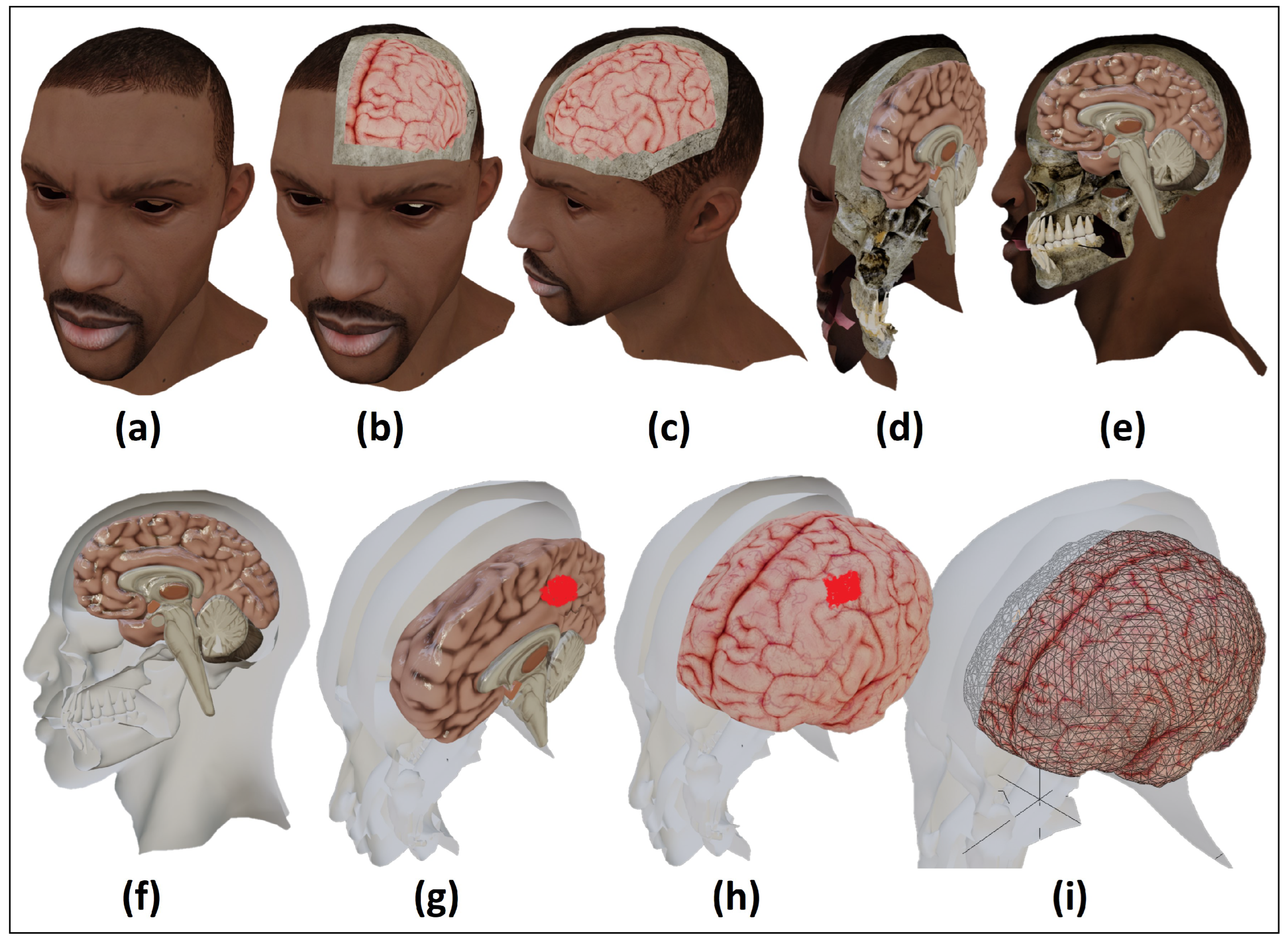
We model a source identification problem [4,5,18], with a source in the brain (Figure 1g,h) and measurements (EEG) recorded on the scalp. We consider the EEG to be produced by large neuron conglomerates simultaneously activated (bioelectrical sources) [4,6]. Moreover, we assume the electric currents produced in the region ${\Omega }_1$ are caused only by the brain’s electrical activity. Such currents are classified as ohmic and primaries. The former is produced by the movement of ionic charges across the extracellular fluid in the brain and the latter by the diffusion currents along the neural membranes denoted by ${\mathbf{J}}^P$ [1,6] (main scope in the identification problem). Such membranes give additional information regarding the affected zone location (Figure 1h). We illustrate this in the 3D models in Figure 1a–e, where we show the skull, brain, and scalp. In Figure 1a, we show a human with short hair in the same scalp region. In Figure 1b,c, we show a cut in the left region displaying the frontal and parietal lobes, respectively. In Figure 1d,e, we show a rotation and transversal cut of Figure 1c, displaying the inner regions of the brain, skull, and scalp separately, and, in Figure 1f, we show the skull and scalp in white, and the inner brain region in colors, with two contrasting regions.

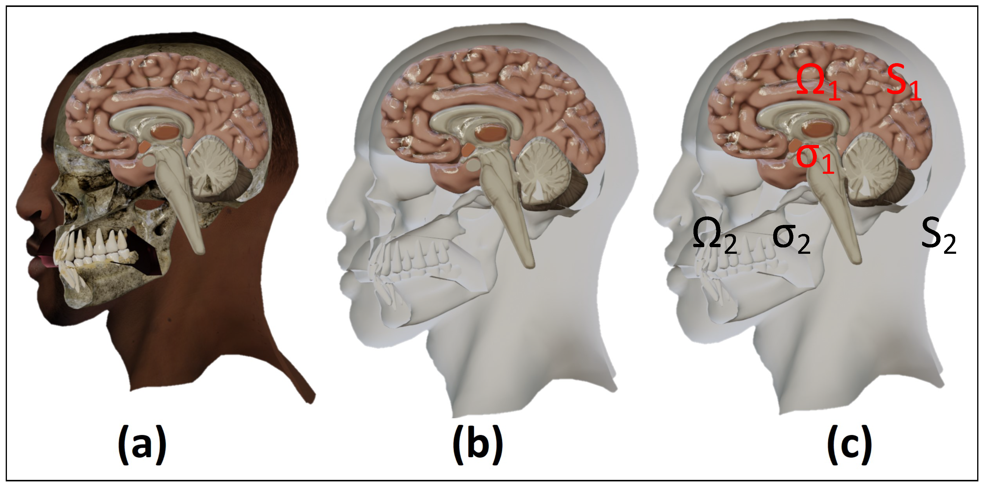
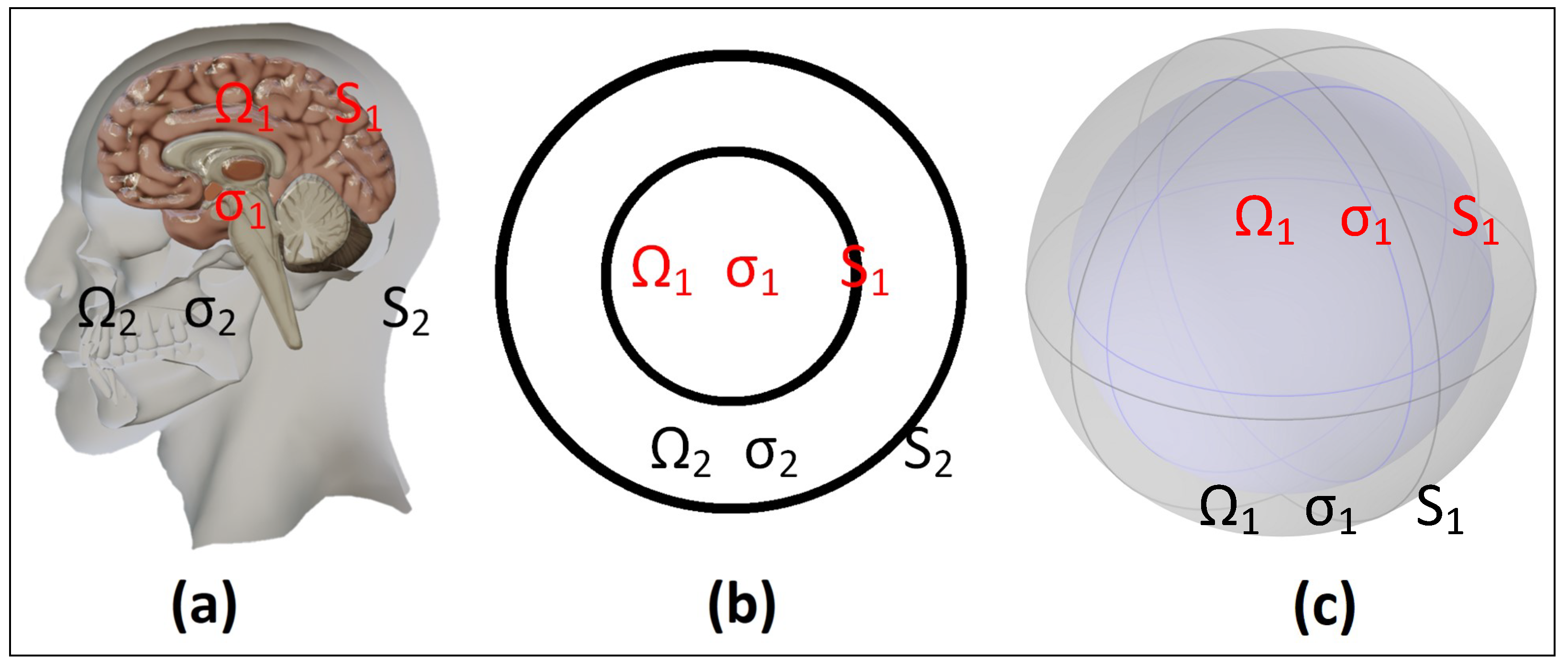
Without loss of generality, we consider the human head as a conductor medium split into two disjoint regions [19], as seen in Figure 2c, with region 1 constituted by the brain, 2 by the light-tone color region (scalp and skull) in Figure 1f (where $\Omega =\overline{{\Omega }_1}\cup {\Omega }_2$) ${\Omega }_1$ is the cerebral cortex and ${\Omega }_2$ is the rest of the head. We can apply this idealization to our construction, which could be further extended to consider additional layers to illustrate the rest of the tissues introducing electrical noise, interference, or modifying the signal coming from the source (inside ${\Omega }_1$). As we mentioned before, the electric activity of the brain is generated by the ionic interchange of a conglomerate of neurons activated simultaneously, and this electrical activity is recorded using electrodes located on the scalp in a EEG (electroencephalogram) [1,4,6,13,14,18,20,21,22]. The ionic interchange of this conglomerate produces a current density called the bioelectrical sources and is denoted by ${\mathbf{J}}^P$ (the primary current). The Electroencephalographic Inverse Problem (IEP) consists of finding, from the EEG, the bioelectrical sources that produces such EEG. The presence of this density current generates electromagnetic potentials associated with the vector fields $\mathbf{E}$, and $\mathbf{B}$ which are coupled [23]. From experimental data, it has been found that the corporal tissues can be regarded as a resistive medium for frequencies up to one Hertz since the capacitive impedance is extremely small [1,4,5,23]. Hence, we can neglect the displacement current in the Maxwell equations. Thus, the Ampere–Maxwell law can be written in the following form: $\nabla \times \mathbf{B}=\mathbf{J}$ with $\mathbf{H}$ the magnetic induction field. Taking the divergence of both sides of the equation, we obtain $\nabla ·\mathbf{J}=\mathbf{0}$ (describing the steady-state of the system). These equations represent the quasi-static model [4,5,23].

The bioelectrical sources cannot radiate a considerable amount of energy since the observation and the source size are considerably smaller than the wavelength associated with the higher frequency produced by bioelectrical processes in the brain. These signals behave as slowly varying signals, and therefore we can consider $\frac{\partial \mathbf{B}}{\partial t}=0$, i.e., we can neglect the variations of $\mathbf{B}$ on time t. Hence, from the previous results and the Faraday law, we obtain $\nabla \times \mathbf{E}=\mathbf{0}$, considering $\mathbf{E}=-\nabla \mathbf{U}$ with $\mathbf{E}$ a conservative field. According to cerebral tissues’ linearity and homogeneity properties, the currents in any instant depend on the sources at such time and obey the superposition law. Hence, formally we can express the total current as a superposition of a current associated with the primary source ${\mathbf{J}}^P$ and the one due to the presence of the electric field $\mathbf{E}$ in the brain region with conductivity $\sigma$ ($\sigma$ is used to generalize the process, since there is a ${\sigma }_i$ conductivity for each region ${\Omega }_i$, with $\Omega =\overline{{\Omega }_1}\cup {\Omega }_2$) leading to ${\mathbf{J}}^T={\mathbf{J}}^P+\sigma \mathbf{E}$, where ${\mathbf{J}}^P$ denotes a primary current, $\sigma$ represents the ohmic current (in both cases density of current), and ${\sigma }_i$ represents the constant conductivity of the region ${\sigma }_i$ ($i=1,2$). Hence, in the region ${\Omega }_1$ (which represents the brain), the potential u satisfies

$$\nabla ·\left(\nabla u\right)=\frac{\nabla ·{\mathbf{J}}^P}{{\mathbf{\sigma }}_{\mathbf{1}}},$$

(1)

from which we obtain $\Delta u=f$, where $f=\frac{1}{{\sigma }_1}\nabla ·{\mathbf{J}}^P$. In the region ${\Omega }_2$, there are no bioelectrical sources, and the potential satisfies the Laplace equation. On the surface $S_1$ separating the homogeneous regions, the boundary conditions correspond to the transmission conditions

$$u_1=u_2;{\sigma }_1\frac{\partial u_1}{\partial {\mathrm{n}}_1}={\sigma }_2\frac{\partial u_2}{\partial {\mathrm{n}}_1},\mathrm{on}{S}_1.$$

(2)

Since the air conductivity is zero, we obtain

$$\frac{\partial u_2}{\partial {\mathrm{n}}_2}=0,\mathrm{on}{S}_2.$$

(3)

Finally, the potential u satisfies the following boundary value problem:

$$\Delta u_1=f\mathrm{in}{\Omega }_1,$$

(4)

$$\Delta u_2=0\mathrm{in}{\Omega }_2,$$

(5)

$$u_1=u_2\mathrm{on}{S}_1,$$

(6)

$${\sigma }_1\frac{\partial u_1}{\partial {\mathrm{n}}_1}={\sigma }_2\frac{\partial u_2}{\partial {\mathrm{n}}_1}\mathrm{on}{S}_1,$$

(7)

$$\frac{\partial u_2}{\partial {\mathrm{n}}_2}=0\mathrm{on}{S}_2.$$

(8)

The EEG is related to the potential u in the following form (t-fixed) $EEG=u_2{\mid }_{S_2}$. Thus, if we consider the constant conductivities ${\sigma }_1$ and ${\sigma }_2$ in ${\Omega }_1$ and ${\Omega }_2$, respectively, the brain cortex $S_1$, and the scalp $S_2$, we can have a suitable representation of Figure 1 and in the following boundary problem, the Electroencephalographic Inverse Problem (EIP) [4,18,24], described in Equations (4)–(8) (where $u_i=u{\mid }_{{\Omega }_i}$, i.e., $u_i$ is the electric potential in ${\Omega }_i$ for $i=1,2$, n${}_i$ the unitary vector normal to the region ${\Omega }_i$, $\Delta$ the Laplacian operator and $f=\mathrm{div}\left({\mathbf{J}}^p/{\sigma }_1\right)$).

The boundary conditions in Equations (6) and (7) are the so-called transmission equations or conditions, and we obtain Equation (8) considering the conductivity of ${\Omega }^C$ as zero (the air conductivity). From Green’s formulae [9,17,24], we deduce the following compatibility condition

$${\int }_{{\Omega }_1}f=0.$$

(9)

The cerebral cortex has a thickness varying from $1.5$ mm to $4.5$ mm. Hence, from the point of view of mathematical modeling, the cerebral cortex can be considered as a 3D-space surface. Thus, the bio-electrical sources generated in the cerebral cortex, not only dipolar sources, can be regarded as functions defined on the mentioned surface. Therefore, the boundary condition associated with the $S_2$ current fluxes reflects the presence of cortical sources. Following the notation used for the volumetric sources, we denote the cortical current density by ${\mathbf{J}}^{\mathbf{p}}$. Hence, the boundary condition is given by:

$${\sigma }_1\frac{\partial u_1}{\partial {\mathrm{n}}_1}={\sigma }_2\frac{\partial u_2}{\partial {\mathrm{n}}_1}+{\mathbf{J}}^{\mathbf{p}}·{\mathrm{n}}_1\mathrm{on}{S}_1,$$

(10)

with ${\mathbf{J}}^{\mathbf{p}}·{\mathrm{n}}_1$ the cortical source, satisfying a compatibility condition similar to Equation (9). Moreover, if we consider simultaneously cortical and volumetric sources, the compatibility condition is given by

$${\int }_{{\Omega }_1}f+{\int }_{{\partial \Omega }_1}{\mathbf{J}}^{\mathbf{p}}·{\mathrm{n}}_1=0.$$

(11)

To build a simplification of the EIP, we analyze the identification problem of the source f, using the boundary problem described in Equations (4)–(8) along with the boundary condition $u_2=V$, considering only volumetric sources, and we neglect the presence of cortical sources. Hence:

Definition 1.

The inverse problem associated with Equations (4)–(8) (EIP) consists of determining a source f from a measurement V defined over $S_2$, such as the solution u of the direct problem corresponding to the source f, satisfying $u{\mid }_{S_2}=V$.

3. Simplification of the Electroencephalographic Inverse Problem

3.1. Operational Statement

We present some results. In the first place, we consider the following spaces

$$\mathcal{U}=\left\{f\in L_2\left({\Omega }_1\right):{\int }_{S_1}fd{S}_1=0\right\}=L_2\left(S_1\right)/\mathbb{R},$$

(12)

$$\mathcal{V}=\left\{u\in H^1(\Omega ):{\int }_{\Omega }ud\Omega =0\right\}=H^1(\Omega )/\mathbb{R},$$

(13)

$$\mathcal{W}=\left\{v\in L_2\left(S_2\right):{\int }_{S_2}vd{S}_2=0\right\}=L_2\left(S_2\right)/\mathbb{R}.$$

(14)

Definition 2.

Let $f\in \mathcal{U}$, the function $u\in \mathcal{V}$ is the so-called weak solution to the Problems (4)–(8) if it satisfies

$${\sigma }_1{\int }_{{\Omega }_1}\nabla u_1·\nabla vdx+{\sigma }_2{\int }_{{\Omega }_2}\nabla u_2·\nabla vdx={\int }_{{\Omega }_1}fvdx,$$

(15)

$\forall v\in H^1(\Omega )$.

Theorem 1 is related to the existence and uniqueness of the weak solution. Its proof can be found in [13].

Theorem 1.

Let f be a function such that $f\in \mathcal{U}$, and the condition in Equation (9) is necessary and sufficient for the existence of a weak solution to the described problem in Equations (4)–(8). The weak solution is unique if $u\in \mathcal{V}$, i.e., u satisfies ${\int }_{\Omega }u\left(x\right)dx=0$. Furthermore, ${\parallel u\parallel }_{H^1(\Omega )}\le C{\parallel f\parallel }_{L_2\left(S_1\right)}$, where the constant C does not depend on the function f.

Taking into account the existence and uniqueness of the solution to the described problem in Equations (4)–(8), we can define the operator $T:\mathcal{U}\to \mathcal{V}$, with $T\left(f\right)=u$. This operator is continuous, as follows from the inequality in Theorem 1. The composition of the continuous operator T and the trace operator $Tr:\mathcal{V}\to \mathcal{W}$ (a compact operator) define a compact operator $A:\mathcal{U}\to \mathcal{W}$ given by $A=Tr\circ T$, i.e., $A\left(f\right)={\left.u\right|}_{S_2}$, whose kernel is described in the Theorem 2:

Theorem 2.

Let $H_1\left({\Omega }_1\right)$ be a subspace of harmonic functions in ${\Omega }_1$ orthogonal to constant functions. Hence, ${\left[KerA\right]}^{\perp }=H_1\left({\Omega }_1\right)$ holds.

Theorem 3 allows us to apply regularization methods for handling the numerical instability present in this problem. The proof of the Theorem is in the work by Fraguela et al. [13].

Theorem 3.

$Im\left(A\right)$ is dense in $L_2\left(S_2\right)$.

Thus, the operator A allows us to study the shortcomings of the inverse identification problem [13].

3.2. Simplified Electroencephalographic Inverse Problem

We can reduce the model describing the EIP to a homogeneous region by using a harmonic function $u_2$ determined by the following Cauchy problem [7,9,24]:

$$\Delta u_2=0,\mathrm{in}{\Omega }_2$$

(16)

$$u_2=V,\mathrm{on}{S}_2$$

(17)

$$\frac{\partial u_2}{\partial {\mathrm{n}}_2}=0,\mathrm{on}{S}_2.$$

(18)

To determine $\overline{u}$, we consider

$$\Delta \overline{u}=0,\mathrm{in}{\Omega }_1$$

(19)

$$\frac{\partial \overline{u}}{\partial {\mathrm{n}}_2}=\psi ,\mathrm{on}{S}_1,$$

(20)

where $\psi =\frac{{\sigma }_2}{{\sigma }_1}\frac{\partial u_2}{\partial {\mathrm{n}}_2}{\mid }_{S_1}$, and $\overline{u}$ is orthogonal to the constants. Hence, the uniqueness of the solution holds if the compatibility condition is satisfied according to $\psi$. The condition is given by ${\int }_{S_1}\psi \left(s\right)ds$ (deduced from Green’s formulae) [9,17,24]. As the last step, we consider the following inverse problem: To determine a source function f satisfying the following boundary value problem

$${\sigma }_1\Delta \widehat{u}=f\mathrm{in}{\Omega }_1,$$

(21)

$${\sigma }_1\frac{\partial \widehat{u}}{\partial \mathrm{n}}=0\mathrm{in}{S}_1,$$

(22)

for $\widehat{u}{\mid }_{S_1}=g=\varphi -\overline{u}{\mid }_{S_1}$ and $\varphi =u_2{\mid }_{S_2}$. From the previous arguments, we can solve the EIP using the inverse problem in a homogeneous region set by Equations (21) and (22), which we call the Simplified Electroencephalographic Inverse Problem (SEIP). We are considering the problem in a homogeneous region. Hence, we can use the Green’s function to find a solution to the problem described in Equations (21) and (22). Thus:

Definition 3.

The so-called Green’s function of the boundary problem described in Equations (21) and (22) is a function $G(y,x)$ satisfying the following boundary problem:

$$\Delta G\left(y,x\right)=\delta \left(y-x\right)-\frac{1}{m\left(\Omega \right)},y,xin\Omega ,$$

(23)

$${\left.\frac{\partial G}{\partial \mathrm{n}}\right|}_S=0,x\in S=\partial \Omega ,y\in \Omega ,$$

(24)

with $m(\Omega )$ the volume of the region Ω.

${\Omega }_1$ represents one of the simple geometries mentioned at the beginning (for example), a circle of radius $R=R_1$. Green’s function is given by

$${\Delta }_{x}G\left(y,x\right)=\delta \left(x-y\right)-\frac{1}{\pi {R_1}^2},\mathrm{in}\Omega ,$$

(25)

$$\frac{\partial G\left(x,y\right)}{\partial \mathrm{n}}=0,\in \partial {\Omega }_1,$$

(26)

with a solution given by

$$G\left(x,y\right)=\frac{1}{2\pi }\left\{\ln \left|x-y\right|+\ln \left|x\overline{y}-{R_1}^2\right|-\frac{{\left|x\right|}^2+{\left|y\right|}^2}{2{R_1}^2}\right\},$$

(27)

where $\overline{y}$ is the complex conjugate of y. From the previous arguments and considering Definition 3, we establish the following Theorem (Theorem 4), regarding the solution representation in terms of Green’s functions. The proof of Theorem (Theorem 4) is in the references [24,25,26].

Theorem 4.

If $f\in C_0^{\perp }$, then the classic solution u of the SEIP is given by

$$u\left(x\right)={\int }_{\Omega }G\left(y,x\right)f\left(y\right)dy,$$

(28)

with G the Green’s function satisfying the problem in Equations (25) and (26).

4. EIP Considering Dipolar Sources

Determining the distributions describing the bioelectrical sources (given the neural activity) is not an easy task. Several techniques and methods have been applied to simplify this problem. For instance, from the previous simplification (SEIP), we can consider a current dipole (a dipolar model of equivalent current) already validated as an accurate representation of sources (shallow sources) inside the brain [13,14,20,21,22,27]. Hence, we can extend the analysis beyond more complex systems with multiple dipoles of the equivalent current type. In this sense, we illustrate the previously mentioned arguments with models simulating epileptic foci using several dipoles or multipolar expansions. Therefore, we consider a single dipole [4], representing the source function f, and at the same time

$$f=\frac{1}{{\sigma }_1}\mathrm{div}\left(\mathbf{P}\delta \left(x-a\right)\right),$$

(29)

with P the dipolar moment and $\delta \left(x-a\right)$ the Dirac delta centered at a [17,24]. If the current is given by ${\mathbf{J}}^p=\mathbf{P}\delta \left(x-a\right)$, the existence’s proof of the boundary problem solution is carried out using Theorem 4 as follows: There exists a succession of continuous functions $f_n$ converging to the Dirac delta. Moreover, there exists the solution $u_n$ of the boundary problem, for each element in the functions succession $\mathrm{div}\left(\mathbf{P}{f}_n\right)$. Such a succession $u_n$ converges to the solution to the problem described in Equations (21) and (22), with

$$u_n\left(x\right)={\int }_{\Omega }G\left(y,x\right)f_n\left(y\right)dy.$$

(30)

Since ${lim}_{n\to \infty }{u}_n$ exists and does not depend on the convergence of the succession to f, we will refer to such a limit as the solution to the boundary problem described in Equations (21) and (22). Thus, if f is given by Equation (29), the solution is

$$u\left(x\right)={\left.\left[\left(\frac{\mathbf{P}}{{\sigma }_1}\right)·\left({\overrightarrow{▽}}_{y}G\left(y,x\right)\right)\right]\right|}_{y=a},$$

(31)

with $G(x,y)$ the Green’s function of the problem. In this case, we have a unique solution to the inverse problem if the measurement V is well-known over all the scalp [9,28,29]. Hence, if we know V, we can recover the parameters of the dipolar source, i.e., the dipolar momentum P and its location a, using the least squares method [9,29]

$$\underset{\mathbf{P},a}{\min }\left({∥\widehat{u}\left(x\right)-f∥}^2\right),$$

(32)

with $\widehat{u}$ the solution of the problem described in Equations (21) and (22), f given by Equation (29), and $\widehat{u}$ expressed in terms of the source f. We bear in mind the inconveniences of using the Green’s function method [9,17,24] for explicitly determining the functions in complex geometries. Generally speaking, if there are edges where we cannot apply the Green’s method [17], we can use the ideas presented in this work, to develop an algorithm to ease the determination of the Green’s functions and hence the solution.

5. Development of the Model Using Simple Geometries

5.1. Concentric Circles Model

In order to validate the ideas laid out in Section 4, we need in the first place to provide a solution to the direct problem. Hence, we consider the human head modeled with two concentric circumferences, as shown in Figure 3a,b, to obtain an exact solution without using numerical methods. The previously stressed arguments are crucial for building examples to validate the Simplification of the EIP (SEIP) to a problem defined in a homogeneous region. The results of this section can be extended (in the circumference case) to concentric spheres, considering that we will require to compute numerically some integrals associated with the Fourier coefficient of the solution (solution of the direct problem). Hence, we conclude that geometries with certain complexity as spherical ones can be solved with our proposed method, requiring, however, numerical methods to solve the direct and inverse problems associated with the phenomenon. Even in such a case, the proposed method offers several advantages in reducing the required computations. According to the ideas stressed in this work, we can reduce the inverse problem to a circular homogeneous region problem using the aforementioned Green’s function method [9,17,24].

5.2. Direct Problem Solution

To find a solution to the direct problem, we consider the following auxiliary boundary problem (similar to the boundary problem described in Equations (4)–(8)

$$\Delta {\omega }_1(r,\theta )=0\mathrm{in}{\Omega }_1,$$

(33)

$$\Delta {\omega }_2(r,\theta )=0\mathrm{in}{\Omega }_2,$$

(34)

$${\omega }_1(r,\theta )={\omega }_1(r,\theta )-g\mathrm{in}{S}_1,$$

(35)

$${\sigma }_1\frac{\partial {\omega }_1}{\partial {\mathrm{n}}_1}(r,\theta )={\sigma }_2\frac{\partial {\omega }_2}{\partial {\mathrm{n}}_1}(r,\theta )\mathrm{in}{S}_1,$$

(36)

$$\frac{\partial {\omega }_2}{\partial {\mathrm{n}}_2}(r,\theta )=0\mathrm{in}{S}_2,$$

(37)

with $g\left(x\right)=\widehat{u}\left(x\right)={\left.\left[\left(\frac{\mathbf{P}}{{\sigma }_1}\right)·\left({\overrightarrow{▽}}_{y}G\left(y,x\right)\right)\right]\right|}_{y=a}$ and $x\in S_1$. The solution of the direct problem described in the boundary problem in Equations (33)–(37) is unique and orthogonal to the constants space [9,24]. Hence, the solution to the problem is given by:

$$u\left(x\right)=\left\{\begin{array}{cc}\widehat{u}+{\omega }_1& x\in {\Omega }_1\\ {\omega }_2& x\in {\Omega }_2\end{array}\right.,$$

(38)

considering $G(x,y)$ given in Equation (27) and the model in Equations (33)–(37), we compute the solution applying the Fourier series method [16,17], obtaining an equations system from the coefficients and substituting the variable values in the proper regions. Thus,

$${\omega }_1(r,\theta )=\sum _{k=1}^{\infty }\left[a_k^1{r}^{k}cos\left(k\theta \right)+b_k^1{r}^{k}sin\left(k\theta \right)\right],$$

(39)

$${\omega }_2(r,\theta )=\sum _{k=1}^{\infty }\left\{\left[a_k^2{r}^k+b_k^2{r}^{-k}\right]cos\left(k\theta \right)+\left[c_k^2{r}^k+d_k^2{r}^{-k}\right]sin\left(k\theta \right)\right\},$$

(40)

with ${\omega }_1$ and ${\omega }_2$ expressed as Fourier series [16], with $a_k^1$ and $b_k^1$ the coefficients of ${\omega }_1$; $a_k^2$, $b_k^2$, $c_k^2$ and $d_k^2$ the coefficients of ${\omega }_2$. Furthermore, we consider Equation (35), with $g\left(\theta \right)={\sum }_{k=1}^{\infty }\left[g_k^{1}cos\left(k\theta \right)+g_k^{2}sin\left(k\theta \right)\right]$ (with coefficients $g_k^1$ and $g_k^2$), to determine if the coefficients satisfy

$${\sigma }_1{g}_k^1=\left({\sigma }_1-{\sigma }_2\right)a_k^2{R_1}^k+\left({\sigma }_1+{\sigma }_2\right)b_k^2{R_1}^{-k},$$

(41)

$${\sigma }_1{g}_k^2=\left({\sigma }_1-{\sigma }_2\right)c_k^2{R_1}^k+\left({\sigma }_1+{\sigma }_2\right)d_k^2{R_1}^{-k},$$

(42)

with $r\to R_1$ in ${\Omega }_1$ or $S_1$. If $r\to R_2$ in ${\Omega }_2$ or $S_2$, we can finally verify that the coefficients in Equations (39) and (40) are given by

$$\left\{\begin{array}{c}{a}_k^2=\frac{{\sigma }_1{g}_k^1{R_1}^k}{\left({\sigma }_1-{\sigma }_2\right){R_1}^{2k}+\left({\sigma }_1+{\sigma }_2\right){R_2}^{2k}},c_k^2=\frac{{\sigma }_1{g}_k^2{R_1}^k}{\left({\sigma }_1-{\sigma }_2\right){R_1}^{2k}+\left({\sigma }_1+{\sigma }_2\right){R_2}^{2k}},\hfill \\ b_k^2=\frac{{\sigma }_1{g}_k^1{R_1}^k{R_2}^{2k}}{\left({\sigma }_1-{\sigma }_2\right){R_1}^{2k}+\left({\sigma }_1+{\sigma }_2\right){R_2}^{2k}},d_k^2=\frac{{\sigma }_1{g}_k^2{R_1}^k{R_2}^{2k}}{\left({\sigma }_1-{\sigma }_2\right){R_1}^{2k}+\left({\sigma }_1+{\sigma }_2\right){R_2}^{2k}},\end{array}\right.$$

(43)

$$a_k^2=\frac{{\sigma }_1{g}_k^1\left({R_1}^{2k}+{R_2}^{2k}\right)}{{R_1}^k\left[\left({\sigma }_1-{\sigma }_2\right){R_1}^{2k}+\left({\sigma }_1+{\sigma }_2\right){R_2}^{2k}\right]}-\frac{g_k^1}{{R_1}^k},$$

(44)

$$b_k^2=\frac{{\sigma }_1{g}_k^2\left({R_1}^{2k}+{R_2}^{2k}\right)}{{R_1}^k\left[\left({\sigma }_1-{\sigma }_2\right){R_1}^{2k}+\left({\sigma }_1+{\sigma }_2\right){R_2}^{2k}\right]}-\frac{g_k^2}{{R_1}^k}.$$

(45)

The coefficients in Equations (43)–(45) are the solution to the problem described in Equations (33)–(37). Without loss of generality, we can consider that the experimental measurement (EEG) is given by $V={\sum }_{k=1}^{\infty }\left[V_k^{1}cos\left(k\theta \right)+V_k^{2}sin\left(k\theta \right)\right]$, with its corresponding coefficients given by

$$V_k^1=g_k^1\frac{{\sigma }_1{g}_k^1{R_1}^k{R_2}^k}{\left({\sigma }_1-{\sigma }_2\right){R_1}^{2k}+\left({\sigma }_1+{\sigma }_2\right){R_2}^{2k}},$$

(46)

$$V_k^2=g_k^g\frac{{\sigma }_1{g}_k^1{R_1}^k{R_2}^k}{\left({\sigma }_1-{\sigma }_2\right){R_1}^{2k}+\left({\sigma }_1+{\sigma }_2\right){R_2}^{2k}},$$

(47)

computing the Fourier expansion of the function $g={\left.\left[\left(\frac{\mathbf{P}}{{\sigma }_1}\right)·\left({\overrightarrow{▽}}_{y}G\left(y,x\right)\right)\right]\right|}_{y=a}$. To this aim, we obtain in the first place ${\overrightarrow{▽}}_{y}G\left(y,x\right)$ with G given by Equation (27):

$${\overrightarrow{▽}}_{y}G\left(y,x\right)=\frac{x-y}{\left|x-y\right|{}^2}+\frac{y}{{R_1}^2}+\frac{1}{\left|x-y\right|{}^2}\left(\left[A_{\partial G_1}{x}_1+B_{\partial G_2}{x}_2\right],\left[A_{\partial G_1}{x}_2-B_{\partial G_2}{x}_1\right]\right),$$

(48)

with $A_{\partial G_1}=x_1{y}_1+x_2{y}_2+{R_1}^2$ and $B_{\partial G_2}=y_1{x}_2-y_2{x}_1$. If we consider the electric dipole (representing the epileptic foci, P $=(p_1,p_2)$), we find the following expression for g

$$g\left(x\right)={\left.\frac{p_1}{{\sigma }_1{\left|x-y\right|}^2}\left\{C_{xy}g+\left(x_1-y_1\right)\right\}+\frac{p_2}{{\sigma }_2{\left|x-y\right|}^2}\left\{C_{xy}^{t}g+\left(x_2-y_2\right)\right\}\right|}_{y=a},$$

(49)

with $C_{xy}g=A_{\partial G_1}{x}_1+B_{\partial G_2}{x}_2$ and $C_{xy}^{t}g=A_{\partial G_1}{x}_2+B_{\partial G_2}{x}_1$. Considering the orthogonality between constant functions and the solution, we can neglect some terms, such as $\frac{y_1}{{R_1}^2}$ and $\frac{y_2}{{R_1}^2}$; denoting $x_1=R_1\cos \left(\theta \right)$, $x_2=R_1\sin \left(\theta \right)$, $y_1=r\cos \left({\theta }_y\right)$ and $y_2=r\sin \left({\theta }_y\right)$ and substituting them into Equation (49), we obtain

$$g\left(x\right)=\frac{p_1\left(1-{R_1}^2\right)}{{\sigma }_1{\left|x-y\right|}^2}\left[R_1\cos \left(\theta \right)-r\cos \left({\theta }_y\right)\right]+\frac{p_2\left(1-{R_1}^2\right)}{{\sigma }_2{\left|x-y\right|}^2}\left[R_1\sin \left(\theta \right)-r\sin \left({\theta }_y\right)\right].$$

(50)

Thus, the Fourier coefficients of g are

$$\begin{array}{cc}\hfill g_k^1& =p_1\frac{\left(1-{R_1}^2\right)\pi {r_0}^{k-1}}{{\sigma }_1{R_1}^{k-2}\left({R_1}^2-{r_0}^2\right)}\left[{r_0}^2\cos \left(\left(k+1\right){\theta }_y\right)+{R_1}^2\cos \left(\left(k-1\right){\theta }_y\right)\right]\hfill \\ \hfill & +p_2\frac{\left(1-{R_1}^2\right)\pi {r_0}^{k-1}}{{\sigma }_2{R_1}^{k-2}\left({R_1}^2-{r_0}^2\right)}\left[{r_0}^2\sin \left(\left(k+1\right){\theta }_y\right)+{R_1}^2\sin \left(\left(k-1\right){\theta }_y\right)\right]\hfill \\ \hfill & -\left(\frac{p_1\cos \left({\theta }_y\right)}{{\sigma }_1}+\frac{p_2\sin \left({\theta }_y\right)}{{\sigma }_2}\right)\frac{\left(1-{R_1}^2\right)2\pi {r_0}^{k+1}\cos \left(k{\theta }_y\right)}{{R_1}^{k-2}\left({R_1}^2-{r_0}^2\right)},\hfill \end{array}$$

(51)

$$\begin{array}{cc}\hfill g_k^2& =p_1\frac{\left(1-{R_1}^2\right)\pi {r_0}^{k-1}}{{\sigma }_1{R_1}^{k-2}\left({R_1}^2-{r_0}^2\right)}\left[{r_0}^2\sin \left(\left(k+1\right){\theta }_y\right)+{R_1}^2\sin \left(\left(k-1\right){\theta }_y\right)\right]\hfill \\ \hfill & +p_2\frac{\left(1-{R_1}^2\right)\pi {r_0}^{k-1}}{{\sigma }_2{R_1}^{k-2}\left({R_1}^2-{r_0}^2\right)}\left[{r_0}^2\cos \left(\left(k+1\right){\theta }_y\right)+{R_1}^2\cos \left(\left(k-1\right){\theta }_y\right)\right]\hfill \\ \hfill & -\left(\frac{p_1\cos \left({\theta }_y\right)}{{\sigma }_1}+\frac{p_2\sin \left({\theta }_y\right)}{{\sigma }_2}\right)\frac{\left(1-{R_1}^2\right)2\pi {r_0}^{k+1}\sin \left(k{\theta }_y\right)}{{R_1}^{k-2}\left({R_1}^2-{r_0}^2\right)}.\hfill \end{array}$$

(52)

We include the procedure to obtain Equations (51) and (52) in Appendix A. The restriction of the function ${\omega }_2$ on $S_2$ gives us the solution to the direct problem. In order to solve the inverse problem, we require the solution of the direct problem. We use COMSOL and MATLAB to obtain the solutions of the direct and inverse problems and to compare the results. Moreover, we consider the quasi-static model to generate a temporal variation of the EEG (or generate an EEG). We need to solve the direct problem at each time. We consider a moment in a time interval as a partition (segment or step) of the time interval where the EEG is measured. For the purposes of this work, we consider the time interval given by $t=[0,1]$. We will divide this interval conveniently. We recall that the brain frequencies are below 64 Hz [1,6]. Thus, by virtue of the Nyquist theorem, we propose a number of divisions multiple of 64, for example, 128 division of time interval t, [30,31]. Moreover (to validate the computation times as well), we propose 64, 128, 256, and 512 divisions of the time interval to compare results of the computation time and obtained error, comparing both the model and recovered sources. The latter allows us to obtain the largest information set regarding our proposal (the problem simplification and the iterative algorithm). We did not include the time in the model. However, it is straightforward to introduce it when considering the solution evolution at each time, obtaining a solution for each time. Hence, we denote by $f_{t_i}=f(x,t_i)$, $x\in {\Omega }_1$, and $u_{t_i}=u(x,t_i)$, $x\in \Omega$, $i=1,\dots ,256$. Thus, we build an algorithm, considering the solution of the boundary problem using the least-squares method, our simplification proposal, and the solution at each time. The algorithm returns the recovered source as the inverse problem solution. The algorithm also compares the source considered in the boundary problem (model source) with the recovered source. We describe this algorithm in Figure 4 and indicate the equations considered in each iteration. The described flowchart can be used to build other algorithms generalizing the methods to solve the boundary problem (an original conductive medium problem for different layers or our simplification) using the Fourier series method [9,17], finite element method [24,26], or any other method. Moreover, the time integration to the solution is performed straightforwardly in the iteration considering the solution of the inverse problem at each time.

Thus, in Figure 5a–h, we show the boundary problem solution (simplified, in COMSOL) of a single region described in Equations (21) and (22) (reduced in Equations (8)–(33) with its solution in Equations (51) and (52) for the 2D and 3D cases in Figure 5a,b, respectively. We show the original boundary problem for two regions described in Equations (4)–(8) for the 2D case and 3D case in Figure 5e,f, respectively. We also show the solution (in Matlab) of the direct problem with its solution restricted to the boundary ($\widehat{u}{\mid }_{\Omega \left(z\right)}$) in two different points over the boundary for $z=x$ in Figure 5c and $z=-x$ in Figure 5g. We point out that the solutions for the simplified case $\widehat{u}{\mid }_{\Omega \left(z\right)}$ with normal $u{\mid }_{\Omega \left(z\right)}$, and z in the equatorial disk in the 2D and 3D cases are similar with a dispersion value of $1\times {10}^{-5}$. Thus, the originally simplified modeled problem (2D and 3D) is equivalent or has acceptable dispersion values. On the other hand, we show the solution to the direct problem (Matlab) to the 3D case of two regions, placing z in the poles. Hence, in Figure 5d, we show $\widehat{u}{\mid }_{\Omega \left(z\right)}$ with $z=y$, and in Figure 5h for $z=-y$. Considering both the regions, the radius value is 1, and the conductivity 2, for region 1, whereas, for region 2, the radius value is $1.2$ and conductivity 1, for both the 2D and 3D case, at a single time.

6. Inverse Problem Solution

To solve the inverse problem, we consider $\mathbf{P}=[-1,1]$ (dipolar moment), for the function $\delta \left(x-a\right)\approx \frac{1}{M_{\beta }}exp\left(-\frac{{\beta }^2}{{\beta }^2-{\left|x-a\right|}^2}\right)$, if $\left|x-a\right|<\beta$, and 0 in other case with x and a vectors (Equation (29)). $M_{\beta }$ is the normalization constant $M_{\beta }={\int }_{{\Omega }_1}^{}exp\left(-\frac{{\beta }^2}{{\beta }^2-{\left|x-a\right|}^2}\right)dx$ with $x\in {\Omega }_1$. Therefore, without loss of generality, we can assume the measurement is given by $V={\sum }_{k=1}^{\infty }\left[V_k^{1}cos\left(k\theta \right)+V_k^{2}sin\left(k\theta \right)\right]$. Following the previously described procedure, we determine function $u_2$ as the solution of the Cauchy problem in ${\Omega }_2$ from V. Hence, we obtain

$$u_2(r,\theta )=\frac{1}{2}\sum _{k=1}^{\infty }\left\{V_k^1{H}_{rR}cos\left(k\theta \right)+V_k^2{H}_{rR}sin\left(k\theta \right)\right\},$$

(53)

with $H_{rR}={\left(\frac{r}{R_2}\right)}^k+{\left(\frac{R_2}{r}\right)}^k$. Subsequently, we determine the harmonic function $\overline{u}$ in ${\Omega }_1$, orthogonal to the constants, such as the Neumann condition $\frac{\partial \overline{u}}{\partial {\mathrm{n}}_1}=\psi =\frac{{\sigma }_2}{{\sigma }_1}\frac{\partial u_2}{\partial {\mathrm{n}}_1}{\mid }_{S_1}$ holds. Such a function is given by

$$\overline{u}=\frac{{\sigma }_2}{2{\sigma }_1}\sum _{k=1}^{\infty }{\left(\frac{r}{R_1}\right)}^k\left[{\left(\frac{R_1}{R_2}\right)}^k-{\left(\frac{R_2}{R_1}\right)}^k\right]\left[V_k^{1}cos\left(k\theta \right)+V_k^{2}sin\left(k\theta \right)\right],$$

(54)

the measurement (simulation of a given experiment or experimental data) g in $S_1$ should satisfy

$$g=\frac{1}{2}\sum _{k=1}^{\infty }\left[{\left(\frac{R_1}{R_2}\right)}^k\left(1-\frac{{\sigma }_2}{{\sigma }_1}\right)+{\left(\frac{R_2}{R_1}\right)}^k\left(1+\frac{{\sigma }_2}{{\sigma }_1}\right)\right]\left[V_k^{1}cos\left(k\theta \right)+V_k^{2}sin\left(k\theta \right)\right].$$

(55)

We emphasize that the Fourier coefficients of g are expressed in terms of $V_k^1$ and $V_k^2$ (Equation (55)). On the other hand, these coefficients are given in terms of the dipolar source parameters P and a. Finally, we should determine the dipole parameters P and a from the measurement V (EEG), using the least-squares method [13,14,20,21,22]. Thus, if we assume the coefficients $V_k^1$ and $V_k^2$ are known, we only require to minimize the functional

$$\underset{\mathbf{P},a}{\min }\sum _{k=1}^{\infty }{\left(g_k^1-{\tilde{g}}_k^1\right)}^2+{\left(g_k^2-{\tilde{g}}_k^2\right)}^2,$$

(56)

with ${\tilde{g}}_k^1$ and ${\tilde{g}}_k^2$ Fourier coefficients approximations of g from Equation (55) ($g_k^1$ and $g_k^2$ in Equations (51) and (52). We can obtain the measurement over the whole scalp if the measurement (EEG) is performed in a finite number of points in the scalp (electrodes) [1,3,6,8]. Such measurement can be obtained using an interpolation regularized method as that presented by Bustamante et al. [32] or the spherical splines interpolation method presented by Perrin et al. [33]. Simple geometries had been used to analyze the electroencephalographic inverse problem (EIP). However, in the case of dipolar sources, several methods have been presented to find their location—for example, in the work by Clerc et al. [34] considering rational approximations in the complex plane and the work by Tsitsas et al. [15], where an algorithm for finding the dipole from the Cauchy data are developed, considering the human head as a spherical model, similar to the extension of a case we have addressed in this work.

7. Numerical Examples

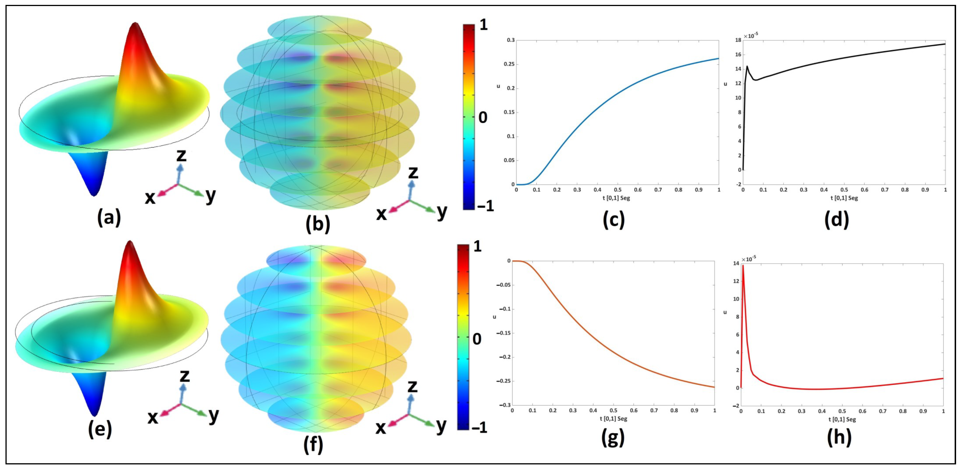
We present numerical (synthetic) examples aiming to illustrate the ideas presented in this work. We consider $R_1=1.2$, $R_2=2$, ${\sigma }_1=3$ and ${\sigma }_2=1$, as well as a dipolar source such as P $=[-1,1]$ (Equation (29)) in Equations (46), (47), (A2) and (A3). We compute the measurement V corresponding to the EEG (simulated according to the conditions in this work at time $t=[0,1]$, see Figure 5c,d,g,h). The computations are performed under the numerical consideration of the model, with a mesh containing some parameters (similar to the finite element), as we show in Figure 1i, recalling that the anomaly is located as in Figure 1g or Figure 1h. On the other hand, we consider the inherent error of the measurement $V^{\delta }$ due to the equipment, randomly related to the Fourier coefficients of V such that ${∥V-V^{\delta }∥}_{L_2\left(S_2\right)}<\delta$, as well as the generalized error, for a suitable $\delta$, a random number Rand, and the errors $E_k^1$ and $E_k^2$, associated with the Fourier coefficients $V_k^1$ and $V_k^2$, given by

$$Error=\sum _{k=1}^{\infty }{E}_k^1{\left(Rand\right)\left(\right|V|}_{max})\sqrt{(}6\delta )cos\left(k\theta \right)+E_k^2{\left(Rand\right)\left(\right|V|}_{max})\sqrt{(}6\delta )sin\left(k\theta \right)$$

(57)

Considering this, we have the approximation to the function g given by:

$$g^{\delta }=\frac{1}{2}\sum _{k=1}^{\infty }\left[{\left(\frac{R_1}{R_2}\right)}^k\left(1-\frac{{\sigma }_2}{{\sigma }_1}\right)+{\left(\frac{R_2}{R_1}\right)}^k\left(1+\frac{{\sigma }_2}{{\sigma }_1}\right)\right]\left[V_k^{1,\delta }cos\left(k\theta \right)+V_k^{2,\delta }sin\left(k\theta \right)\right]$$

(58)

for the 2D case. On the other hand, for the 3D case, we consider the source $(x^2-y^2)z$. We can analyze this source in spherical coordinates as $\frac{r^3}{2}\left[1-cos\left(2\varphi \right)\right]cos\left(\varphi \right)cos\left(2\theta \right)$. We apply the previously described theory to solve the direct problem considering two regions, to simplify the problem to one region as well (as we have described through this work). In this case, the solution of the direct problem obtained as the restriction of the solution of the boundary value problem of two 3D regions, using the Fourier series method [17] is given by:

$$V\left(\theta ,\varphi \right)=\frac{14{\sigma }_1{R_1}^9{R_2}^3\sqrt{2\pi }}{\left[4\left({\sigma }_2-{\sigma }_1\right){R_1}^7-\left(4{\sigma }_2+3{\sigma }_1\right){R_2}^7\right]27\sqrt{105}}\left[Y_{2,3}\left(\theta ,\varphi \right)+Y_{3,2}\left(\theta ,\varphi \right)\right],$$

(59)

with Y the spherical harmonics [9,17] for a solution $u\left(r,\theta ,\varphi \right)$ in ${\Omega }_1$ of the form

$$u\left(r,\theta ,\varphi \right)=\sum _{n=0}^{\infty }\sum _{m=n}^n\left[a_{nm}^1{r}^n+b_{nm}^1{r}^{n+2}\right]Y_{nm}\left(\theta ,\varphi \right),$$

(60)

and in ${\Omega }_2$

$$u\left(r,\theta ,\varphi \right)=\sum _{n=0}^{\infty }\sum _{m=n}^n{a}_{nm}^2{r}^n{Y}_{nm}\left(\theta ,\varphi \right),$$

(61)

In this case, the error is given by

$$Error=\sum _{n=0}^{\infty }\sum _{m=n}^n\frac{a_{nm}{\left(Rand\right)}_{nm}\left({\left|V\right|}_{max}\right)\sqrt{6\delta }}{n\pi \sqrt{2n+1}}{Y}_{nm}\left(\theta ,\varphi \right).$$

(62)

In what follows, we consider the parameters described at the beginning of this section ($R_1=1.2$, $R_2=2$, ${\sigma }_1=3$ and ${\sigma }_2=1$). For the numerical experiments, we use COMSOL and MATLAB to solve the direct problems. We use scripts developed by us (in MATLAB) to solve the problems using circular and spherical harmonics. To minimize the functional in Equation (56), we use the fminunc Matlab function.

The previously stressed ideas can be used in more realistic geometries of the head along with numerical methods, such as the finite differences and finite element methods.

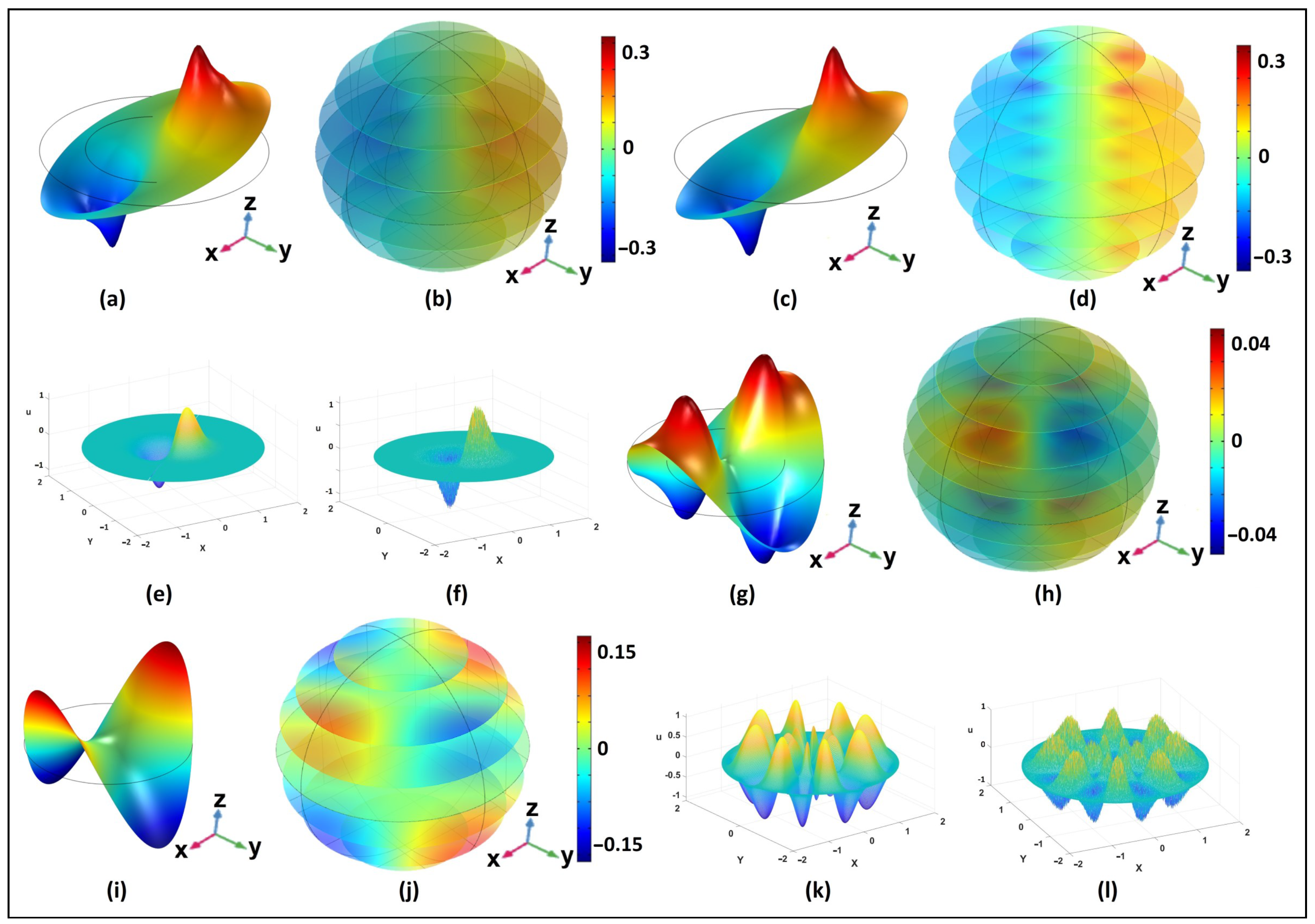
In Figure 6, we show the solutions to the boundary problems as well as that to the direct and inverse problems for the numerical examples previously mentioned in Section 7. In Figure 6a–d, we show the solution to the boundary problem for the dipolar source in Figure 6a,b for the two regions 2D and 3D cases, respectively. In Figure 6c,d, we show the simplified 2D and 3D cases, respectively. In Figure 6e,f, we show the source recovered solution from solving the inverse problem, respectively. In Figure 6g–j, we show the boundary problem for the source $(x^2-y^2)z$, in Figure 6g,h, the two regions 2D and 3D cases, respectively, whereas, in Figure 6i,j, the simplified case for the 2D and 3D, respectively. In Figure 6k,l, we show the source and the recovered solution from solving the inverse problem. The errors obtained between the exact and recovered sources were $0.018$ for the dipolar source case, and $0.019$ for the source $(x^2-y^2)z$. In

Table 1. Software comparison. Computation times in minutes and seconds (min:sec) for the two used software: Matlab and COMSOL, obtained when solving the multiple layer conductive medium problem (original) and using our simplification proposal (reduced). We tested these methods when solving two different sources: one computed from the dipolar momentum P = [−1, 1] and the other one from the expression $f=(x^2-y^2)z$. We show the percentage error (%) and the absolute error (A) between the exact and recovered sources after solving the inverse problem in time, and dividing the time interval in 64, 128, 256, and 512 parts (each division corresponds to a moment in time). DTI (Divisions of the time interval): M (Matlab), C (Comsol)—in the last column: O (Original), R (Reduced).

DTI	64	Error		128	Error		256	Error		512	Error
		%	A		%	A		%	A		%	A
	Source computed from the EEG with P = [−1, 1], Equation (29)
M	1:32	0.1009	0.0111	2:50	0.0213	0.0015	5:10	0.0201	0.0016	10:11	0.0189	0.0017	O
	0:56	0.0897	0.0095	1:40	0.0185	0.0023	4:10	0.0176	0.0013	8:05	0.0170	0.0012	R
C	2:11	0.0908	0.0081	3:20	0.0205	0.0031	6:15	0.0199	0.0021	15:25	0.0187	0.0021	O
	1:35	0.0789	0.0065	2:10	0.0181	0.0019	5:05	0.0171	0.0020	11:55	0.0167	0.0013	R
	Source computed from $f=(x^2-y^2)z$
M	2:03	0.1111	0.013	3:22	0.0240	0.0031	5:45	0.0223	0.0019	10:57	0.0211	0.0024	O
	1:28	0.0999	0.0087	2:11	0.0190	0.0021	4:52	0.0188	0.0022	8:59	0.0183	0.0016	R
C	2:46	0.0899	0.0093	3:59	0.0214	0.0019	6:57	0.0211	0.0025	16:11	0.0200	0.0018	O
	1:53	0.0700	0.0065	2:31	0.0199	0.0021	5:43	0.0192	0.0015	12:33	0.0180	0.0014	R

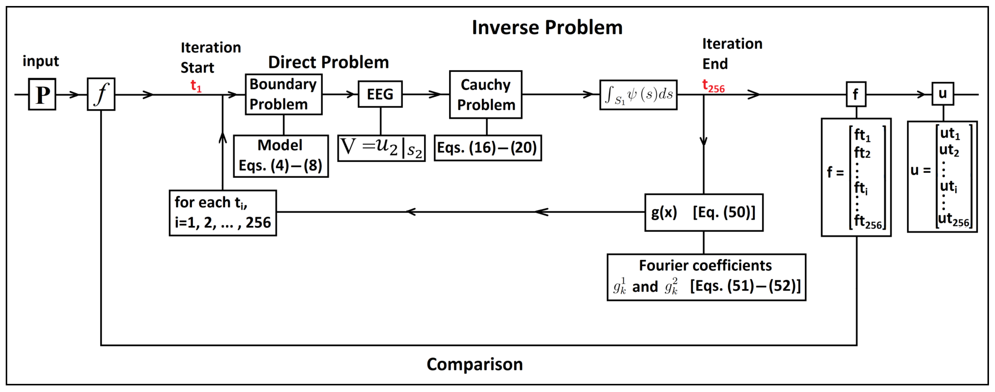
, we show the numerical results from our different comparisons and proposals. We recall that we applied our simplification (reduced) proposal and Fourier series solution in Equations (46) and (47) (obtained as well from Equations (51) and (52)) to solve the inverse problem. Moreover, we solved the two-layers (original) conductive medium problem, comparing in both inverse problems the recovered source. As we mentioned previously, we included time into the problem and subsequently solved both problems, original and reduced, using our algorithm, described in Figure 4, for different time interval divisions (moments in time) of $64,128,256,512$ to compare our results. Among these divisions, we concluded that the time interval $t=[0,1]$ is the most optimal and efficient, as we show in Table 1 having significantly short computation times with respect to other divisions. Moreover, the percentage error (error [%]) between the model source (computed from the dipolar momentum P $=[-1,1]$ in Equation (29) and for $f=(x^2-y^2)z$) and the recovered source (final part of the algorithm shown in Figure 4) validates our proposal as optimal, with a computation time of 2 min in average and an error of $0.02\%$. In Table 1, we also show the computation times for different sources recovered by inverse problems involving the multiple-layers conductive medium problem and our simplification proposal, along with the errors between the model sources and the recovered sources solving the inverse problem using our algorithm at different times.

8. Conclusions

In this work, we study the inverse problem for brain bioelectrical sources using the EEG recorded on the scalp. These sources and the EEG are correlated by a boundary value problem deduced from Maxwell’s equations and the head electrical properties. This boundary value problem is defined in a non-homogeneous region representing the head. We consider the epileptic foci case, i.e., anomalies with no electric characteristic changes in the brain but influencing the triggers’ quantities of the brain cells due to a possible problem in the sodium channels (sodium pathy). We are not considering tumor-associated anomalies such as edemas and calcifications, which have electric characteristic changes in the region they occupy. However, for illustration purposes, we briefly stress the tumor case. In the case of a tumor, the zone occupied by it changes its conductivity, generating a fibrous layer surrounding it. In such a layer, the produced current, i.e., the second current, produces an abnormal EEG. If the layer is considerably thin, it can be considered as the surface separating the region occupied by the anomaly from the healthy brain. In such a case, the generating source of the abnormal EEG can be regarded as a shallow-type source, defined over the separation surface and the boundary condition of the separation interface between the healthy brain and the pathology is given by Equations (6) and (10). On the other hand, if the fibrous layer is thick, the EEG generating source can be considered a volumetric source. In this case, the boundary conditions of separation interface are given by Equations (6) and (7).

We emphasize that, in this work, we are focusing only on the source type identification rather than on its localization since the used space coordinates are an idealization for the models and geometric considerations regarding the skull and head representation. Hence, the localization problem is beyond the scope of this work and will be addressed in a forthcoming article since the simplification can optimize the spatial localization of the source.

We apply a simplification, leading us to a boundary value problem in a homogeneous region. In the simplification, we solve the Cauchy problem for the Laplace equation in an annular region and use the Green’s functions method to reduce the problem to a homogeneous region. We solve the simplified problem in space and included time as an additional variable to solve the phenomenon at different times. We consider a moment in time as the division of the time interval in multiples of the frequency known in the EEG. Hence, we propose an algorithm to analyze the boundary problem, the direct problem solution, and the inverse problem solution at each time, considering the time as the iterations in the algorithm. We summarize the results of our proposal in Table 1. We observe that the optimal times and errors show the highest efficiency for 128 divisions in the time interval with an error of $0.02\%$ and computation time of 2 min in Matlab.

We illustrate the algorithm with sources associated with epilepsy. The latter is one of the most relevant applications of the EEG. In particular, we consider sources associated with epileptic foci. Moreover, the simplicity of the epileptic foci modeling is an attractive example of the dipolar moment application, relating the electromagnetic theory in the sources’ nature and the construction of our bioelectric activity-based proposal. We conclude that our proposal has applications in the identification of this kind of source.

References

1. Fornito, A.; Zalesky, A.; Bullmore, E.T. Fundamentals of Brain Network Analysis. In Biology; Elsevier: Berkeley, CA, USA, 2016. [Google Scholar]
2. Cho, J.; Ibbott, G.; Gillin, M.; Gonzalez-Lepera, C.; Min, C.H.; Zhu, X.; El-Fakhri, G.; Paganetti, H.; Mawlawi, O. Determination of elemental tissue composition following proton treatment using positron emission tomography. Phy. Med. Biol. 2013, 58, 3815–3835. [Google Scholar] [CrossRef] [PubMed] [Green Version]
3. Ravan, M. Beamspace fast fully adaptive brain source localization for limited data sequences. Inverse Probl. 2017, 5, 055021. [Google Scholar] [CrossRef]
4. Sarvas, J. Basic Mathematical and Electromagnetic Concepts of the Biomagnetic Inverse Problem. Phys. Med. Biol. 1987, 32, 11–22. [Google Scholar] [CrossRef]
5. Heller, L. Return Current in Encephalography. Variational Principles. Biophys. J. 1990, 57, 601–606. [Google Scholar] [CrossRef] [Green Version]
6. Nunez, P.L.; Srinivasan, R. Electric Fields of the Brain: The Neurophysics of EEG; Oxford University Press: Oxford, UK, 2006. [Google Scholar]
7. Riley, K.F.; Hobson, M.P.; Bence, S.J. Mathematical Methods for Physics and Engineering: A Comprehensive Guide; Cambridge University Press: Cambridge, UK, 2006. [Google Scholar]
8. Tiumentsev, Y.; Egorchev, M. Neural Network Modeling and Identification of Dynamical Systems; Elsevier Academic Press: London, UK, 2019. [Google Scholar]
9. Glowinski, R.; Neittaanmäki, P. Partial Differential Equations: Modelling and Numerical Simulation. In Computational Methods in Applied Sciences; Springer: Dordrecht, The Netherlands, 2008. [Google Scholar]
10. WHO (World Health Organization). 2019. Available online: https://www.who.int/news-room/fact-sheets/detail/epilepsy (accessed on 20 April 2022).
11. Decker, S.; Roberts, A.; Green, J. LORETA Neurofeedback in College Students with ADHD; Elsevier Academic Pressl: San Diego, CA, USA, 2015; Volume 14, p. 333. [Google Scholar]
12. Conde-Mones, J.; Juárez-Valencia, L.; Oliveros-Oliveros, J.; León-Velasco, D. Stable numerical solution of the Cauchy problem for the Laplace equation in irregular annular regions. Methods Partial Differ. Equ. 2008, 33, 1799–1822. [Google Scholar] [CrossRef]
13. Fraguela, A.; Morín, M.; Conde, J.; Oliveros, J. Inverse electroencephalography for volumetric sources. Math. Comput. Simul. 2008, 78, 481–492. [Google Scholar] [CrossRef]
14. Morín, M.; Netzahualcoyotl, C.; Conde, M.; Oliveros, J.; Santillan, A. Stable Identification of Sources Associated with Epileptic Focus on the Cerebral Cortex. Rev. Mex. Ing. Bioméd. 2019, 40, e201854. [Google Scholar] [CrossRef]
15. Tsitsas, N.; Martin, P. Finding a source inside a sphere. Inverse Probl. 2011, 28, 015003. [Google Scholar] [CrossRef]
16. Downes, J.R.; Faux, D.A. The Fourier-series method for calculating strain distributions in two dimensions. J. Phy. Cond. Matter. 2008, 9, 4509–4520. [Google Scholar] [CrossRef]
17. Dennemeyer, R. Introduction to Partial Differential Equations and Boundary Value Problems; McGraw-Hill: New York, NY, USA, 1968. [Google Scholar]
18. Grave-de-Peralta, R.; González-Andino, S.; Gómez-González, C.M. The biophysical foundations of the localisation of encephalogram generators in the brain. The application of a distribution-type model to the localisation of epileptic foci. Rev. Neurol. 2004, 39, 748–756. [Google Scholar] [PubMed]
19. Rudin, W. Principles of Mathematical Analysis; McGraw-Hill: New York, NY, USA, 1979. [Google Scholar]
20. León-Velasco, D.; Morín, M.; Oliveros, J.; Pérez-Becerra, T.; Escamilla-Reyna, J. Numerical Solution of Some Differential Equations with Henstock–Kurzweil Functions. J. Funct. Spaces 2019, 2019, 8948570. [Google Scholar] [CrossRef]
21. Morín, M.; Netzahualcoyotl, C.; Oliveros, J.; Conde, J.; Juárez, L. Stable identification of sources located on separation interfaces of two different homogeneous media. Ad. Differ. Equ. Control Process. 2019, 20, 53–97. [Google Scholar] [CrossRef]
22. Conde, J.; Estrada, E.; Oliveros, J.; Hernández, C.; Morín, M. Stable Identification of Sources Located on Interface of Nonhomogeneous Media. Mathematics 2021, 9, 1932. [Google Scholar] [CrossRef]
23. Plonsey, R. Bioelectrical Phenomena; McGraw-Hill: New York, NY, USA, 1969. [Google Scholar]
24. Sobolev, S.L. Partial Differential Equations of Mathematical Physics. In Pergamon Press and Addison-Wesley; Elsevier: London, UK, 1964. [Google Scholar]
25. Kress, R. Linear Integral Equations; Springer: New York, NY, USA, 2014. [Google Scholar]
26. Tikhonov, A.N.; Samarskii, A.A. Equations of Mathematical Physics; Oxford Pergamon: Oxford, UK; Dover Publications: Mineola, NY, USA, 2013. [Google Scholar]
27. Muravchik, C.H.; Nehorai, A. EEG/MEC error bounds for a static dipole source with a realistic head model. IEEE Transac. Signal Process. 2001, 3, 470–484. [Google Scholar] [CrossRef]
28. Bogachev, V.I. Measure Theory, Volume I; Springer: Berlin/Heidelberg, Germany, 2007. [Google Scholar]
29. Mood, A.M.F.; Graybill, F.A.; Boes, D.C. Introduction to the Theory of Statistics; McGraw-Hill: New York, NY, USA, 1973. [Google Scholar]
30. Buzáki, G. Rhythms of the Brain; Oxford University Press: Oxford, UK, 2006. [Google Scholar]
31. Sanei, S.; Chambers, J.A. EEG Signal Processing; Jhon Wiley: New York, NY, USA, 2008. [Google Scholar]
32. Bustamante, J.; Castillo, R.; Fraguela, A. A regularization method for polynomial approximation of functions from their approximate values at nodes. J. Numer. Math. 2009, 2, 97–118. [Google Scholar] [CrossRef]
33. Perrin, F.; Pernier, J.; Bertrand, O.; Echallier, J.F. Spherical splines for scalp potential and current density mapping. Electroencephalogr. Clin. Neurophysiol. 1989, 2, 184–187. [Google Scholar] [CrossRef]
34. Clerc, M.; Leblond, J.; Marmorat, J.P.; Papadopoulo, T. Source localization using rational approximation on plane sections. Inverse Probl. 2012, 28, 055018. [Google Scholar] [CrossRef]
35. Arfken, G.B.; Weber, H.J.; Harris, F. Mathematical Methods for Physicists; Elsevier Academic Press: London, UK, 2012. [Google Scholar]
Figure 1. (a) 3D model of a human head; (b) cut in the skull and scalp in the upper-frontal left region to show the frontal and parietal brain lobes; (c) rotation of the cut in (b); (d) transversal cut in (c) to show the inner region of the brain. The skull and scalp are shown as interfaces; (e) profile of (d). (f) The same as (e), contrasting the skull and scalp in white; (g) rotation of (f) showing in red a region in the inner brain zone representing an anomaly; (h) the same as (g), showing the whole brain. We indicate in red a possible anomaly in the brain surface. (i) mesh of the brain, similar to a 3D mesh for applying certain types of numerical methods.
Mathematics 10 01926 g001
Figure 2. (a) 3D model in Figure 1e; (b) 3D model showing the scalp and skull as a single region (region 2) in a light-tone color (similar to white); (c) two different regions 1 and 2, with different conductivities σ 1 and σ 2 , and outer regions S 1 and S 2 , respectively, for the regions Ω 1 and Ω 2 .
Mathematics 10 01926 g002
Figure 3. (a) Two regions model in Figure 2c chosen for representation with two simple regions; (b) 2D representation of the model in (a) with two concentric circles representing regions 1 and 2; (c) 3D representation of the model in (a) with concentric spheres.
Mathematics 10 01926 g003
Figure 4. Algorithm of the proposal in this work, for optimizing the computation times by simplifying the direct problem having an inverse problem solution that allows us to determine the source function and the solution at different times. The algorithm is iterative, with i the number of iterations, depending on the number of points or divisions equal to 64, 128, 256, 512 in the time interval t = [ 0 , 1 ] . The comparison was performed according to the COMSOL problem construction to generate the Matlab code, starting from the geometry construction, the regions or region (due to the problem simplification), boundary conditions, and the mesh quantification in the finite element method.
Mathematics 10 01926 g004
Figure 5. Solution of the problem described in Equations (21) and (22) for the 2D (a) and 3D (b) cases. The solution of the original boundary problem for two regions described in Equations (4)–(8) for the 2D (e) and 3D (f) cases for a single time (at t = 1 seg). We simulate the problem in time to obtain a solution (in Matlab) to u ^ Ω z z = x in Figure 5c and z = x in Figure 5g. Solution of the direct problem (Matlab) for the 3D case of region 1, u ^ Ω z , with z = y in (d), with z = y in (h), with z = x in (c), and with z = x in (g). Considering both the regions, the radii values are 1 and 1.2 , conductivities 2 and 1, for regions 1 and 2, respectively.
Mathematics 10 01926 g005
Figure 6. Solution of the problem described in Equations (21) and (22) (simplified) for the 2D and 3D case for the dipolar source and ( x 2 y 2 ) z , as well as the original boundary problem for two regions described in Equations (4)–(8). (ad) solution of the boundary problem in the dipolar source; (a,b) two regions case; (c,d) simplified 2D and 3D regions case, respectively; (e,f) source and recovered solution from solving the inverse problem; (gj) solution of the boundary problem of the source ( x 2 y 2 ) z ; (g,h) two regions case; (i,j) simplified 2D and 3D case, respectively; (k,l) source and recovered solutions from solving the inverse problem.
Mathematics 10 01926 g006