Optimal Tuning of the Speed Control for Brushless DC Motor Based on Chaotic Online Differential Evolution

Abstract

The efficiency in the controller performance of a BLDC motor in an uncertain environment highly depends on the adaptability of the controller gains. In this paper, the chaotic adaptive tuning strategy for controller gains (CATSCG) is proposed for the speed regulation of BLDC motors. The CATSCG includes two sequential dynamic optimization stages based on identification and predictive processes, and also the use of a novel chaotic online differential evolution (CODE) for providing controller gains at each predefined time interval. Statistical comparative results with other tuning approaches evidence that the use of the chaotic initialization based on the Lozi map included in CODE for the CATSCG can efficiently handle the disturbances in the closed-loop system of the dynamic environment.

1. Introduction

Nowadays, the application of robotic systems in diverse engineering areas is one of the most active fields where science and technology are merged. The inclusion of a robot in a harsh environment involves replacing the human being (regarding tasks) in such a way that the robot controller must have the capability of handling uncertainties to confront unexpected environments [1] and achieve autonomy. As most robot controllers are in a cascade control arrangement, the actuator controller is one of the final inner loops. Therefore, the actuator controller’s adaptability, reconfigurability, and flexibility are vital to handling the task. In this direction, the brushless direct current (BLDC) motor is the most used actuator in industry and commercial applications; it is expected that in the year 2030, BLDC motors will replace the majority of traditional induction motors in the industry [2].

The brushless direct current (BLDC) motor is a permanent magnet synchronous motor that is widely used in diverse applications because it improves the efficiency and control of aerospace processes [3], electric vehicles [4], submarines [5], wind turbines [6], photovoltaic energy [7], etc. Unlike the permanent magnet synchronous motor (PMSM), which has a sinusoidal back-electromagnetic force (back-EMF) wave shape, the BLDC motor has $15\%$ more power density than PMSM [8]. The main difference between the PMSM and the BLDC motor is in the flux distribution in the motor; the BLDC motor is a permanent magnet synchronous motor with a trapezoidal back-EMF wave shape.

On the other hand, the most representative advantages of the BLDC motor compared to the brushed DC motor [9,10] include its high reliability and efficiency, high torque capability, long service life, low maintenance, high speed operating range with the noiseless operation, good dynamic response, and the reduction of size and weight. Those advantages in BLDC motors come from the electronic commutation circuit that replaces the mechanical commutator of brushed DC motors. Hence, the BLDC motor is the most used today.

The efficiency in the regulation and tracking performance of BLDC motors depends on two main aspects, the controller design [8,11] and the controller tuning process [12,13,14,15]. Several PID-like controllers and advanced control strategies have been adopted to address the first aspect. Nevertheless, the controller design does not guarantee to fit one or several performance characteristics, such as settling time, maximum overshoot, steady-state error, energy consumption, etc. The control performance is influenced mainly by the controller tuning process, i.e., the setting of its parameters.

According to the taxonomy of the controller tuning methods given in [16,17], analytic tuning methods find the controller gains by analyzing the closed-loop system stability. Those methods provide suboptimal solutions in nonlinear systems because they only show a region of interest in the controller parameter space, such that a selection procedure must be additionally done in such a region to find the controller gains that fulfill the desired performance characteristics. For instance, in robotic manipulators [18,19], the use of Lyapunov stability defines the conditions to find the PID-like controller gains where the stability is ensured in a specified domain. Likewise, the rule-based procedure in the heuristic tuning methods searches for controller parameters by using the experience in the manual tuning of the controller and the assumptions in the plant and desired output. Some representative heuristic tuning methods are the Tyreus–Luyben method [20], the Cohen–Coon method [21], the Ziegler–Nichols tuning method [22], Ciancone–Marlin method [23], and the C-H-R method [14]. Nevertheless, those methods require more time to tune the controller, which represents a challenge. Moreover, those methods can be applied to a reduced class of systems mainly focused on industrial plants expressed as linear systems; it is also difficult to simultaneously consider several performance indices. In nonlinear systems, the assumptions made in the heuristic tuning methods produce undesired results in the closed-loop system.

Otherwise, the most promising controller tuning approaches are related to the optimization and adaptive methods (according to the taxonomy in [16,17]). In the optimization method and in a class of the adaptive method, the controller tuning is formulated as a dynamic optimization problem, which becomes an NP-hard problem [24], and the solution requires special techniques. The main difference between the optimization and adaptive methods is that the former is stated as an offline dynamic optimization problem, where fixed controller gains are obtained at the end of the optimization process, and those optimum gains are set in the controller for the real-time implementation in a second step. Meanwhile, the latter is formulated as an online dynamic optimization problem, where the controller gains change through time, i.e., the controller is tuned in the closed-loop system. In both cases, the representation of the plant, either by using the approximated mathematical model or the surrogate model (metamodel), is required.

Hence, the intelligent control (IC) [25] for the controller tuning tasks has been frequently used in the optimization method and the adaptive method. The IC [25] in the controller tuning tasks involves systems based on knowledge and rules from the collection of methodologies and techniques of the computational intelligence and soft computing to emulate the decision making of an expert to state the corresponding controller gains. In [26], a novel machine learning technique was incorporated in search of the link–mass parameters used in the controller and the tuning of PID gains. The proposal incorporates a Bayesian optimization that incorporates a surrogate probabilistic model to construct the performance functions from the search parameters, i.e., this model mapping from the design parameters to the objective functions. It does not require the robot model in the approach. A penalty function is incorporated to constrain the joint position error, which results in unstable behaviors. In other work, model-based reinforcement learning (MBRL) in the human–robot collaborative task was used [27]. In that work, the stiffness and damping of the impedance control parameters were found to minimize human effort by using an ensemble of artificial neuronal networks (ANNs) and a model predictive controller.

In the reviewed literature on the use of IC in BLDC motors, the IC was able to reduce (in a better fashion) the torque ripples compared to several control techniques [2]. In the last decade, computational intelligence in the controller tuning task has increased because of the growth of complex demands in real applications that must simultaneously be satisfied. Among the computational intelligence techniques, metaheuristic algorithms [28] have been adopted in the controller tuning problem [12] because they can provide suitable solutions for NP-hard problems.

Several tuning strategies have been adopted in the control system of BLDC motors based on metaheuristic algorithms. In

Table 1. Investigations related to the BLDC motor controller tuning problem using metaheuristic algorithms.

Ref.	Used Controller	Tuning Parameters	Design Objective *	Employed Algorithms	Optimization Process
[10]	PID	PID controller gains	SE	PSO	Offline
[30]	VcPMSMd	Speed and current controller gains, coefficients	SE in the settling phase,	FAMA, GA	Offline and Online
		in the velocity filter and voltage compensators	MO, RT, AxCOsc	Simplex Method
[31]	FL	Membership function parameters	SE, SL	PSO	Online
[32]	PI	PI controller gains	MO, ST, SE	DE, Modified DE	Online
[33]	Online ANFIS, PID,	Learning rate, forgetting factor, steepest descent,	RMSE+IAE+ITAE+ISE	BAT, GA, PSO	Offline
	Fuzzy PID, Adaptive FL	momentum constant, PID, Fuzzy, and FL controller gains
[34]	Fuzzy PID supervised on-line RFNN	Learning rate, dynamic factor, node number	RMSE, IAE, ITAE, ISE	GA, PSO, ACO, BA, ALO	Offline
[35]	PI	PI controller gains	IAE, ISU	PSO with five inertia weight adjustment strategies	Offline
[36]	ANFIS	Learning rate, forgetting factor,	ISE, TDPC	BFO	Offline
		steepest descent momentum constant		BAT, PSO
[37]	PID–type FL	PID controller gains	IAE	GA	Offline
[38]	PID	PID controller gains	ISE	FPA, PSO, FA Ziegler–Nichols	Offline
[39]	PID	PID controller gains	ISE	GOA	Offline
[40]	Fuzzy PD/PID	PD/PID controller gains, membership function parameters, coefficient of the consequent part of fuzzy PD/PID controller	RMSE, IAE, ITAE, ISE	PSO, CS, BAT	Offline
[41]	FOPID	PID controller gains, fractional-orders	RMS	BAT, Modified GA, MSA, ABC	Offline
[42]	FOPI, PI	PI controller gains, fractional-orders	ITAE		Offline
[43]	PI	PI controller gains	MO, ST	GA	Offline
[44]	PID	PID controller gains	ITSE	PSO, BFO	Offline
[45]	FOPD	PI controller gains, fractional-orders	TR	Jaya	Offline
[46]	Online ANFIS, PID, offline ANFIS	Learning rate, forgetting factor, steepest descent momentum constant	RMSE, MO	Hybrid GA-PSO	Offline
[47]	FOPID	PID controller gains, fractional-orders	TR	FA, GA	Offline

* The error is related to the difference between the desired and actual motor velocity.

, the most important features of each work are shown. PID-like controllers are the most used ones in the controller tuning with $42\%$ of the works presented in such a table. This is related to the PID-like controller being the most used in industrial applications in over $90\%$ of systems because of the implementation facility and reduced costs; moreover, when the gains are well-tuned [29], they exhibit somewhat robust performances in nonlinear and time-varying processes, such that the electric drive’s market does not justify the use of the advanced control [30]. Otherwise, neuro-fuzzy-like controllers and PID-like fractional-order controllers present the same use frequency ($21\%$). The rest of the works ($16\%$) in Table 1 include fuzzy logic control. In this work, the PI controller is used for the velocity regulation of the BLDC motor.

The use of the offline optimization process has prevailed in the controller parameter tuning of the BLDC motor with $84\%$ of the works presented in Table 1. However, the offline optimization process is affected by disturbances and uncertainties not considered in the optimization problem, such that the controller tuning may behave differently in real-time implementation. So, robust tuning strategies are required in practical applications [48]. In order to face such an issue in BLDC motors, efforts have been carried out in [33,34,46] to improve the closed-loop system performance under different operating conditions by using lookup tables of controller tuning parameters previously found by the offline optimization process.

The lack of ideal plant models for depicting real-world systems (which are inherently uncertain), the limitations in the offline optimization process to handle complexities, as well as the performance degradation of the closed-loop system appear after some time, giving rise to the use of the online optimization process for controller tuning. However, although the adaptive tuning method could efficiently handle the uncertainties and the disturbances in the closed-loop system compared to an offline optimization process, only $16\%$ of works in Table 1 applied the online optimization process in the tuning problem of the BLDC motor controller. The lack of works may be attributed to the high computational costs in the solution of the online optimization process through metaheuristic algorithms, which is a challenge in real applications. Moreover, the reliability of the adaptive tuning process must be guaranteed in an interest region due to the stochastic nature of the metaheuristic algorithms; nonetheless, the works reported in such a table do not reach conclusions that extend beyond the obtained data.

Contributions

In Table 1, several improvements and applications of metaheuristic algorithms in the speed controller tuning task of the BLDC motor are observed. The most used algorithms are based on particle swarm optimization (PSO) and genetic algorithm (GA). The inclusion of chaotic dynamics [49] in metaheuristics reveals a positive impact of chaotic functions instead of the classic pseudo-random functions. Nevertheless, chaotic dynamics in the solution of the controller tuning task of BLDC motors (by using an online optimization process) are not reported in the literature. The empirical results of this work indicate that the use of chaotic dynamics in the differential evolution algorithm in an online optimization process suitably balances its search capacities, maintaining (as minimum as possible) the motor velocity error under the effects of disturbances.

In this work, different from the research given in Table 1, the chaotic adaptive tuning strategy for controller gains (CATSCG) of BLDC motors is proposed; this is the first contribution of the paper. In the author’s previous works [50,51], the parameters of the inverse dynamic controller (model-based controller) for the speed regulation of the brushed DC electric motor were obtained through a single-stage tuning strategy. In that strategy, it is assumed that a specific closed-loop system response and the obtained control parameters are associated with the DC motor parameters and not the linearizing control parameters. Then, in the best-case scenario, the response of the closed-loop system with the optimum gains will behave as it was established from the beginning. Unlike the author’s previous works, the CATSCG consists of a two-stage tuning strategy where the dynamics associated with the future behavior of the BLDC motor are estimated in the first stage with the experience gained from the past optimization process. These dynamics are used in the second stage to find, through the novel chaotic online differential evolution (CODE), the controller gains that directly impact the closed-loop system responses. Furthermore, the CODE includes Lozi chaotic initial populations in the differential evolution algorithm to enhance the diversity of candidate solutions in the dynamic environment, which further improves the quality of the controller gains under the effects of uncertainties.

On the other hand, unlike what was reported in Table 1, the efficiency of the proposed CATSCG in BLDC motors is shown through the use of nonparametric statistical tests [52] to make inferences from our study data to more general conditions and, hence, to reach general conclusions that extend beyond the obtained data. With this test, the reliability of the proposed control tuning based on metaheuristics in future practical applications is confirmed, providing more fair and meaningful comparative studies with other tuning approaches. The latter is the second contribution of the work.

Based on the above, the novelties of the proposal are summarized next:

• The chaotic online differential evolution is included in the two-stage adaptive tuning strategy for the controller gains. This chaotic adaptive tuning strategy can efficiently handle perturbations, uncertainties, noise, and abrupt changes in the references of the closed-loop system.
• The reliability of the proposed CATSCG in future practical applications is confirmed by presenting a nonparametric statistical study that provides more fair and meaningful comparative studies with other tuning approaches.

The advantages of the proposed chaotic adaptive tuning strategy in the BLDC motors are:

• In a real application (for example, in the object manipulation task), the system (for instance, the robotic manipulator) to be incorporated into the BLDC motor shaft can be modeled as a dynamic load. So, one of the advantages of the proposed chaotic adaptive tuning strategy in the BLDC motors is that this dynamic load could be considered a dynamic perturbation, such that the proposal could handle such perturbation and others (uncertainties, noise, and reference velocity changes) in a better fashion.
• The proposal assumes an analytical model to represent the system dynamics where its efficiency increases, unlike the model-free tuning approaches where the use of machine learning and reinforcement learning estimates the behavior of the system (or performance function), and so, a trade-off between the model accuracy and computational time must be considered. The model-free tuning approaches tend to increase the computational time when they increase the accuracy, while simple ones affect the precision [53] but reduce the computational time.

The rest of the paper is organized as follows. In Section 2, the dynamics and controller of the BLDC motor are presented. The details of the proposed CATSCG of BLDC motors are included in Section 3. The discussion of the results is given in Section 4, and finally, in Section 5, the conclusions are drawn.

2. BLDC Motor Dynamics and Speed Controller

The brushless direct current (BLDC) motors are three-phase synchronous motors usually in a star topology. The schematic diagram of the BLDC motor is shown in Figure 1. The variables associated in the figure include the phase resistance r, the phase inductance l, the friction coefficient $b_0$, the trapezoidal back-electromagnetic (EMF) force $e_{\gamma }$ induced in the winding of phase $\gamma \in \left\{a,b,c\right\}$, the angular position $\theta$, the angular velocity w, the phase to phase voltage $V_{\gamma \gamma }$, the phase voltage $V_{\gamma }$, the phase current $i_{\gamma }$, the load torque ${\tau }_L$, the input voltage $V_s$ and the total torque ${\tau }_e$.

The dynamic equations of the BLDC motor consist of the electrical and mechanical ones [8,11]. The electrical equations are given in (1)–(3), where R and L are the phase-to-phase resistance and inductance, respectively.

$$\begin{array}{ccc}\hfill V_{ab}& =& L\left(\frac{d{i}_a}{dt}-\frac{d{i}_b}{dt}\right)+R\left(i_a-i_b\right)+e_a-e_b\hfill \end{array}$$

(1)

$$\begin{array}{ccc}\hfill V_{bc}& =& L\left(\frac{d{i}_b}{dt}-\frac{d{i}_c}{dt}\right)+R\left(i_b-i_c\right)+e_b-e_c\hfill \end{array}$$

(2)

$$\begin{array}{ccc}\hfill V_{ca}& =& L\left(\frac{d{i}_c}{dt}-\frac{d{i}_a}{dt}\right)+R\left(i_c-i_a\right)+e_c-e_a\hfill \end{array}$$

(3)

The equations in (1)–(3) are influenced by the three-phase full-bridge inverter conduction mode shown in

Table 2. The three-phase full-bridge inverter 120-degree conduction mode.

Switching Interval	Sequence Number	Switch Closed	${\mathit{V}}_{\mathit{aN}}$	Phase Voltage $\raisebox{1ex}{${\mathit{V}}_{\mathit{s}}$}\!\left/ \!\raisebox{-1ex}{$2$}\right.$ ${\mathit{V}}_{\mathit{bN}}$	${\mathit{V}}_{\mathit{cN}}$	Voltage Flowing in Sequence
$0-\raisebox{1ex}{$\pi $}\!\left/ \!\raisebox{-1ex}{$6$}\right.$	1	$Q_5,Q_3$	off	−	+
$\raisebox{1ex}{$\pi $}\!\left/ \!\raisebox{-1ex}{$6$}\right.-\raisebox{1ex}{$\pi $}\!\left/ \!\raisebox{-1ex}{$2$}\right.$	2	$Q_5,Q_1$	+	−	off
$\raisebox{1ex}{$\pi $}\!\left/ \!\raisebox{-1ex}{$2$}\right.-\raisebox{1ex}{$5\pi $}\!\left/ \!\raisebox{-1ex}{$6$}\right.$	3	$Q_6,Q_1$	+	off	−
$\raisebox{1ex}{$5\pi $}\!\left/ \!\raisebox{-1ex}{$6$}\right.-\raisebox{1ex}{$7\pi $}\!\left/ \!\raisebox{-1ex}{$6$}\right.$	4	$Q_6,Q_2$	off	+	−
$\raisebox{1ex}{$7\pi $}\!\left/ \!\raisebox{-1ex}{$6$}\right.-\raisebox{1ex}{$3\pi $}\!\left/ \!\raisebox{-1ex}{$2$}\right.$	5	$Q_4,Q_2$	−	+	off
$\raisebox{1ex}{$3\pi $}\!\left/ \!\raisebox{-1ex}{$2$}\right.-\raisebox{1ex}{$11\pi $}\!\left/ \!\raisebox{-1ex}{$6$}\right.$	6	$Q_4,Q_3$	−	off	+
$\raisebox{1ex}{$11\pi $}\!\left/ \!\raisebox{-1ex}{$6$}\right.-2\pi$	7	$Q_5,Q_3$	off	−	+

, i.e., the current and voltage flowing in the motor windings when the pairs of switches are conducted. Each switch in the inverter conducts (activates) for a duration of $\raisebox{1ex}{$2\pi $}\!\left/ \!\raisebox{-1ex}{$3$}\right.rad=120$°, and the pair of switches are activated in sequence at $\raisebox{1ex}{$pi$}\!\left/ \!\raisebox{-1ex}{$3$}\right.rad=60$°, as shown in Figure 2. In a real application, the switches $Q_1$–$Q_6$ consist of metal-oxide-semiconductor field-effect transistor (MOSFET) devices, which are controlled by PWM signals through the gate driver commutation logic.

The switching sequence mathematical equations of the inverter are included in the phase voltages $V_{aN}=\frac{V_s}{2}\overline{\eta }\left(\theta \right)$, $V_{bN}=\frac{V_s}{2}\overline{\eta }(\theta -2\pi /3)$, and $V_{cN}=\frac{V_s}{2}\overline{\eta }(\theta -4\pi /3)$, considering the inverter commutation function $\overline{\eta }\left(\theta \right)$ expressed in (4). Then, the phase-to-phase voltages $V_{ab}=\frac{V_s}{2}\left(\overline{\eta }\left(\theta \right)-\overline{\eta }(\theta -2\pi /3)\right)$, $V_{bc}=\frac{u}{2}\left(\overline{\eta }(\theta -2\pi /3)-\overline{\eta }(\theta -4\pi /3)\right)$, and $V_{ca}=\frac{u}{2}\left(\overline{\eta }(\theta -4\pi /3)-\overline{\eta }\left(\theta \right)\right)$ include the inverter dynamics, and those are introduced in (1)–(3).

$$\overline{\eta }\left(\theta \right)=\left\{\begin{array}{cc}\hfill 0,& If -\pi /6\le \theta \le \pi /6\\ \hfill 1,& If \pi /6\le \theta \le 5\pi /6\\ \hfill 0,& If 5\pi /6\le \theta \le 7\pi /6\\ \hfill -1,& If 7\pi /6\le \theta \le 11\pi /6\end{array}\right.$$

(4)

The trapezoidal back-EMF force $e_{\gamma }$ is described by (5)–(7), where $k_e$ is the back-EMF constant of the motor and $\overline{e}\left(\theta \right)$ is related to the trapezoidal shape function (due to switch-commutation logic for BLDC motors) displayed in (8).

$$\begin{array}{ccc}{e}_a& =& k_{e}w\overline{e}\left(\theta \right)\end{array}$$

(5)

$$\begin{array}{ccc}\hfill e_b& =& k_{e}w\overline{e}(\theta -2\pi /3)\hfill \end{array}$$

(6)

$$\begin{array}{ccc}\hfill e_c& =& k_{e}w\overline{e}(\theta -4\pi /3)\hfill \end{array}$$

(7)

$$\overline{e}\left(\theta \right)=\left\{\begin{array}{cc}\hfill rl\frac{6\theta }{\pi },& If -\pi /6\le \theta \le \pi /6\\ \hfill 1,& If \pi /6\le \theta \le 5\pi /6\\ \hfill -\frac{6\left(\theta -\pi \right)}{\pi },& If 5\pi /6\le \theta \le 7\pi /6\\ \hfill -1,& If 7\pi /6\le \theta \le 11\pi /6\end{array}\right.$$

(8)

The mechanical equations of the BLDC motor are presented in (9) and (10), where P is the number of pole pairs.

$$\begin{array}{ccc}\hfill J\frac{dw}{dt}+b_{0}w+{\tau }_L& =& {\tau }_e\hfill \end{array}$$

(9)

$$\begin{array}{ccc}\hfill \frac{d\theta }{dt}& =& Pw\hfill \end{array}$$

(10)

The total torque ${\tau }_e$ in (9) results from the sum of the torque applied for each phase, and it is described in (11), where $k_m$ is the torque constant.

$${\tau }_e=k_m\left(i_a\overline{e}\left(\theta \right)+i_b\overline{e}(\theta -2\pi /3)+i_c\overline{e}(\theta -4\pi /3)\right)$$

(11)

Let the state space $x={[\theta ,w,i_a,i_b,\int ({\overline{x}}_2-w)dt]}^T\in R^5$, the desired one $\overline{x}$ and the control signal $u=V_s$ given by the proportional integral (PI) speed controller as

$$u=k_p({\overline{x}}_2-x_2)+k_i{x}_5$$

(12)

Assuming that $i_a+i_b+i_c=0$ and grouping the BLDC motor parameter in the vector $\Theta ={[\frac{b_0}{J},\frac{k_m}{J},\frac{k_e}{L},\frac{R}{L},\frac{1}{L},\frac{1}{J},{\tau }_L]}^T\in R^7$, and the PI control gains in $K={[k_p,k_i]}^T$, the electromechanical BLDC motor dynamics can be expressed in the state space x as follows:

$$\begin{array}{cc}\hfill \dot{x}& =\left[\begin{array}{ccccc}0& P& 0& 0& 0\\ 0& -{\Theta }_1& \overline{C}{\Theta }_2& \overline{D}{\Theta }_2& 0\\ 0& \frac{\overline{A}}{3}{\Theta }_3& -{\Theta }_4& 0& 0\\ 0& \frac{\overline{B}}{3}{\Theta }_3& 0& -{\Theta }_4& 0\\ 0& -1& 0& 0& 0\end{array}\right]x+\left[\begin{array}{cc}0& 0\\ 0& 0\\ \frac{2}{3}{\Theta }_5& \frac{1}{3}{\Theta }_5\\ -\frac{1}{3}{\Theta }_5& \frac{1}{3}{\Theta }_5\\ 0& 0\end{array}\right]\left[\begin{array}{c}{V}_{ab}\\ V_{bc}\end{array}\right]-\left[\begin{array}{c}0\\ {\Theta }_6{\Theta }_7\\ 0\\ 0\\ {\overline{x}}_2\end{array}\right]\hfill \\ \hfill \dot{x}& =f(x,\Theta ,K)\hfill \end{array}$$

(13)

where $\overline{A}=\overline{e}(\theta -2\pi /3)-2\overline{e}\left(\theta \right)+\overline{e}(\theta -4\pi /3)$, $\overline{B}=\overline{e}\left(\theta \right)-2\overline{e}(\theta -2\pi /3)+\overline{e}(\theta -4\pi /3)$, $\overline{C}=\overline{e}\left(\theta \right)-\overline{e}(\theta -4\pi /3)$, $\overline{D}=\overline{e}(\theta -2\pi /3)-\overline{e}(\theta -4\pi /3)$, $V_{ab}=\frac{u}{2}\left(\overline{\eta }\left(\theta \right)-\overline{\eta }(\theta -2\pi /3)\right)$ and $V_{bc}=\frac{u}{2}\left(\overline{\eta }(\theta -2\pi /3)-\overline{\eta }(\theta -4\pi /3)\right)$.

3. Chaotic Adaptive Tuning Strategy for Controller Gains in BLDC Motors

The proposed chaotic adaptive tuning strategy for controller gains (CATSCG) of BLDC motors consists of the adaptive tuning strategy with two sequential stages and a novel chaotic online differential evolution (CODE) algorithm. In the first stage, the CATSCG fits the BLDC motor parameters $\tilde{\Theta }\left(t\right)$ of a model based on an identification stage. In the second stage, the CATSCG settles the parameters $K\left(t\right)$ of the controller based on a predictive stage using the trained model. Finally, both stages are settled as dynamic optimization problems where the proposed CODE obtains the corresponding solutions to set those parameters at each predefined fixed time interval through time.

In this formulation, the time t is split in the time sequence ${\{t_0,t_l\}}_{l\in \mathbb{N}}$ with $\mathbb{N}:=\{1,2,\dots ,n_{\mathbb{N}}\}$. At each time sequence, the information about the actual BLDC motor states is provided by integrating its dynamics (13), considering the time interval between two consecutive times, $\Delta t=t_l-t_{l-1}>0$, as the integration step. In a real application, $\Delta t$ refers to the sampling time, and the actual states are acquired through sensors. On the other hand, the proposed CATSCG is carried out at each discrete time sequence $\overline{t}\in {\{{\overline{t}}_0,{\overline{t}}_{\overline{l}}\}}_{\overline{l}\in \overline{\mathbb{N}}}$ with $\overline{\mathbb{N}}:=\{1,2,\dots ,n_{\overline{\mathbb{N}}}\}$, where the time interval between two tuning processes is expressed as $\Delta \overline{t}={\overline{t}}_{\overline{l}}-{\overline{t}}_{\overline{l}-1}>\Delta t$.

In the time $t<\Delta w=n_w\Delta t$ considering $n_w\ge 1$, the initial parameter values of the controller $K\left({\overline{t}}_0\right)$ and the BLDC motor model parameters $\tilde{\Theta }\left({\overline{t}}_0\right)$ are chosen by the user. The model parameter vector $\tilde{\Theta }\left(t\right)$ of the BLDC motor model and the controller parameter one $K\left(t\right)$ are updated based on the identification and predictive stages at each time $t={\overline{t}}_{\overline{l}}$. In those stages, the actual BLDC motor state information and the BLDC motor model in the backward/forward time window $\Delta w$ are required in the CATSCG. The visual representation of the proposed parameter adaptation in the CATSCG is shown in Figure 3, and the time horizon for the updating of the parameters $\tilde{\Theta }\left(t\right)$ and $K\left(t\right)$ is displayed in Figure 4.

One of the main aims of using CODE in the adaptive tuning strategy is to provide the most suitable model parameter $\tilde{\Theta }\left(t\right)$ and control gains $K\left(t\right)$ at each time $t={\overline{t}}_{\overline{l}}$, such that they achieve an appropriate future behavior of the closed-loop system in the next time interval $t\in ({\overline{t}}_{\overline{l}},{\overline{t}}_{\overline{l}+1}]$, and so the controller can efficiently handle the uncertainties in the system.

The requirements to apply the CATSCG are: (I) The structure of BLDC motor dynamics must be known and described by differential equations. (II) The transcription method [54] is used to apply the proposed CODE or other optimizers. This method transforms the original continuous time formulation (infinite-dimensional optimization problem) into a discrete time formulation (discrete-dimensional optimization problem). The associated dynamics are set as finite states through the solution of the differential equations by numerical integration techniques. Moreover, there is a control system parameterized in the corresponding control gains. (III) The solution of the optimization process in the CATSCG at each time $t=\overline{t}$ must be computed in the time interval between two tuning processes (in $\Delta \overline{t}s$) for real-time implementations of CATSCG in a prototype.

The following subsections detail the optimization problem formulation of the CATSCG for identifying and predicting stages and present the proposed chaotic online differential evolution that solves both problems.

3.1. Identification Stage in the BLDC Motor

In the identification stage, the parameter vector $\tilde{\Theta }\left(t\right)\in R^7$ of the BLDC motor model is fitted at each time ${\overline{t}}_{\overline{l}}$ through the solution of a dynamic optimization problem. The identification stage requires the actual BLDC motor state information from a short backward time interval. This time interval is set as $t\in \tilde{\Omega }\in [{\overline{t}}_{\overline{l}}-▵w,{\overline{t}}_{\overline{l}}]$. In this stage, the dynamic equations of the BLDC motor model are expressed in (16), where $\tilde{x}\left(t\right)$ is the model state vector.

The dynamic optimization problem consists of finding the parameter vector ${\tilde{\Theta }}^{*}\left({\overline{t}}_{\overline{l}}\right)$ of the BLDC motor dynamics (16), which minimizes the identification error $J_I\in R$ (14) between the actual states $x\left(t\right)$ and the model ones $\tilde{x}\left(t\right)$.

$$J_I\left(\tilde{t}\right)={\left(x_1\left(\tilde{t}\right)-{\tilde{x}}_1\left(\tilde{t}\right)\right)}^2+{\left(x_2\left(\tilde{t}\right)-{\tilde{x}}_2\left(\tilde{t}\right)\right)}^2+{\left(x_3\left(\tilde{t}\right)-{\tilde{x}}_3\left(\tilde{t}\right)\right)}^2+{\left(x_4\left(\tilde{t}\right)-{\tilde{x}}_4\left(\tilde{t}\right)\right)}^2$$

(14)

The dynamic optimization problem’s mathematical formulation of the identification stage is presented in (15)–(18) in the time interval $t\in \tilde{\Omega }\in [{\overline{t}}_{\overline{l}}-▵w,{\overline{t}}_{\overline{l}}]$. This problem is constrained by the BLDC motor model (16) with its final conditions (17), and the bound interval $[{\tilde{\Theta }}_{min},{\tilde{\Theta }}_{max}]$ (18) of the parameter vector $\tilde{\Theta }$. A backward numerical integration method [55] is used to the solution of the differential equation of the motor model.

$$\begin{array}{c}\begin{array}{c}min\\ {\tilde{\Theta }}^{*}\left({\overline{t}}_{\overline{l}}\right)\in R^7\end{array}{\int }_{t\in \tilde{\Omega }}{J}_I\left(t\right)dt\end{array}$$

(15)

Subject to:

$$\begin{array}{c}\dot{\tilde{x}}=\left[\begin{array}{ccccc}0& P& 0& 0& 0\\ 0& -{\tilde{\Theta }}_1& \overline{C}{\tilde{\Theta }}_2& \overline{D}{\tilde{\Theta }}_2& 0\\ 0& \frac{\overline{A}}{3}{\tilde{\Theta }}_3& -{\tilde{\Theta }}_4& 0& 0\\ 0& \frac{\overline{B}}{3}{\tilde{\Theta }}_3& 0& -{\tilde{\Theta }}_4& 0\\ 0& -1& 0& 0& 0\end{array}\right]\tilde{x}+\left[\begin{array}{cc}0& 0\\ 0& 0\\ \frac{2}{3}{\tilde{\Theta }}_5& \frac{1}{3}{\tilde{\Theta }}_5\\ -\frac{1}{3}{\tilde{\Theta }}_5& \frac{1}{3}{\tilde{\Theta }}_5\\ 0& 0\end{array}\right]\left[\begin{array}{c}{V}_{ab}\\ V_{bc}\end{array}\right]-\left[\begin{array}{c}0\\ {\tilde{\Theta }}_6{\tilde{\Theta }}_7\\ 0\\ 0\\ {\overline{x}}_2\end{array}\right]\end{array}$$

(16)

$$\begin{array}{c}\tilde{x}\left({\overline{t}}_{\overline{l}}\right)=x\left({\overline{t}}_{\overline{l}}\right)\end{array}$$

(17)

$$\begin{array}{c}{\tilde{\Theta }}_{min}\le \tilde{\Theta }\left({\overline{t}}_{\overline{l}}\right)\le {\tilde{\Theta }}_{max}\end{array}$$

(18)

The minimization of the identification error through the optimization process provides a trained model that approximates, through the model parameters ${\tilde{\Theta }}^{*}\left({\overline{t}}_{\overline{l}}\right)\in R^7$, the dynamic behavior of the actual BLDC motor.

3.2. Predictive Stage in the BLDC Motor

In the predictive stage, the controller gains $K\left(t\right)\in R^2$ of the PI speed controller are obtained in the time ${\overline{t}}_{\overline{l}}$ by using the trained model as a state predictor, and solving a dynamic optimization problem in the time interval $t\in \widehat{\Omega }\in [{\overline{t}}_l,{\overline{t}}_l+\Delta w]$. The state predictor $\widehat{x}$ of the BLDC motor computes the estimated future motor behavior, and the acquired information from this behavior is given through the forward numerical integration of the differential equation of the trained model in the short time interval $t\in \widehat{\Omega }$. The dynamics of the predictor (trained model) are given in (21), and so, it uses the BLDC motor model parameter vector ${\tilde{\Theta }}^{*}\left({\overline{t}}_{\overline{l}}\right)$ found in the previous identification stage.

The predictive error $J_p\in R$ (19) between the predictive state of the motor speed ${\widehat{x}}_2$ and the reference one ${\overline{x}}_2$ is chosen as the performance function to be optimized.

$$J_p\left(\widehat{t}\right)={({\overline{x}}_2\left(\widehat{t}\right)-{\widehat{x}}_2\left(\widehat{t}\right))}^2$$

(19)

The formulation of the dynamic optimization problem for the predictive stage is shown in (20)–(25). The aim was to find the control gains $K^{*}\left({\overline{t}}_{\overline{l}}\right)\in R^2$ based on the minimization of the predictive error, subject to the predictive state equations (trained model) (21) with its initial conditions (23) and the predictive controller (22) using $V_{ab}=\frac{\widehat{u}}{2}\left(\overline{\eta }\left(\theta \right)-\overline{\eta }(\theta -2\pi /3)\right)$, $V_{bc}=\frac{\widehat{u}}{2}\left(\overline{\eta }(\theta -2\pi /3)-\overline{\eta }(\theta -4\pi /3)\right)$; the bounds of both the control signal (24) and control gains (25). The subscript in (24) and (25) indicate the minimum and maximum values of the related term.

$$\begin{array}{cc}\hfill & \begin{array}{c}min\\ K{\left({\overline{t}}_{\overline{l}}\right)}^{*}\in R^2\end{array}{\int }_{t\in \widehat{\Omega }}{J}_p\left(t\right)dt\end{array}$$

(20)

Subject to:

$$\begin{array}{c}\begin{array}{c}\dot{\widehat{x}}=\left[\begin{array}{ccccc}0& P& 0& 0& 0\\ 0& -{\tilde{\Theta }}_1& \overline{C}{\tilde{\Theta }}_2& \overline{D}{\tilde{\Theta }}_2& 0\\ 0& \frac{\overline{A}}{3}{\tilde{\Theta }}_3& -{\tilde{\Theta }}_4& 0& 0\\ 0& \frac{\overline{B}}{3}{\tilde{\Theta }}_3& 0& -{\tilde{\Theta }}_4& 0\\ 0& -1& 0& 0& 0\end{array}\right]\widehat{x}+\left[\begin{array}{cc}0& 0\\ 0& 0\\ \frac{2}{3}{\tilde{\Theta }}_5& \frac{1}{3}{\tilde{\Theta }}_5\\ -\frac{1}{3}{\tilde{\Theta }}_5& \frac{1}{3}{\tilde{\Theta }}_5\\ 0& 0\end{array}\right]\left[\begin{array}{c}{V}_{ab}\\ V_{bc}\end{array}\right]-\left[\begin{array}{c}0\\ {\tilde{\Theta }}_6{\tilde{\Theta }}_7\\ 0\\ 0\\ {\overline{x}}_2\end{array}\right]\end{array}\end{array}$$

(21)

$$\begin{array}{c}with\widehat{u}=k_p({\overline{x}}_2-{\widehat{x}}_2)+k_i{\widehat{x}}_5\end{array}$$

(22)

$$\begin{array}{c}\widehat{x}\left({\overline{t}}_{\overline{l}}\right)=x\left({\overline{t}}_{\overline{l}}\right)\end{array}$$

(23)

$$\begin{array}{c}{\widehat{u}}_{min}\le \widehat{u}\left(t\right)\le {\widehat{u}}_{max}\end{array}$$

(24)

$$\begin{array}{c}{K}_{min}\le K\left({\overline{t}}_{\overline{l}}\right)\le K_{max}\end{array}$$

(25)

The decrement of the predictive error through the optimization process provides the PI control gains that fulfill the regulation task in the prediction time horizon. At the end of this stage, the optimum controller parameter vector $K^{*}\left({\overline{t}}_{\overline{l}}\right)$ is set to the control system in (12) for the velocity regulation of the actual BLDC motor in the next time interval $[{\overline{t}}_{\overline{l}}-{\overline{t}}_{\overline{l}+1}]$.

3.3. Chaotic Online Differential Evolution

As mentioned before, the adaptive optimal tuning of the speed control for the brushless DC motor requires the solution of two consecutive optimization problems online, i.e., the problems are solved at every $\Delta \overline{t}$ during the execution of the speed regulation task in the motor: the identification problem (to estimate the current motor parameters) and the prediction one (for the tuning of the speed controller). Both problems are complex and must be solved fast. This section details the optimizer used for this purpose.

The proposed chaotic online differential evolution (CODE) is an optimizer based on the variant DE/rand/1/bin of differential evolution. It incorporates a chaotic initialization and an elitist adaptation mechanism to improve the exploitative capacity and the speed convergence of the original algorithm. The components of CODE are described next.

3.3.1. Differential Evolution

Differential evolution (DE) is a well-known bio-inspired, population-based, and approximated optimizer that is shown to be effective when solving complex optimization problems, especially those involved in real-world applications as observed in the recently specialized literature [56,57,58]. This method is bio-inspired in the process of natural evolution and was proposed by Storn and Price in 1997 [59].

DE follows the operation described in Algorithm 1. This optimizer starts with a random population ${\mathrm{X}}^G$ that contains $NP$ vectors (candidate solution vectors to the optimization problem). Then, these vectors evolve iteratively through a given number of generations $G_{max}$ to find a suitable approximated solution to the problem. An offspring population is generated using mutation and crossover operations for each generation. After that, a selection procedure decides which solutions must survive from this new population and the original one for the next iteration based on a fitness function (the value of the objective function and the compliance with constraints in the optimization problem). By the end of the algorithm, the population includes the fittest vectors, and the best one is the solution to the problem.

Algorithm 1: Differential evolution (DE)

DE includes different variants that can be useful to address different types of optimization problems. Each variant aims to enhance two features of the algorithm—the exploration (the ability to find promising regions in the search space) and the exploitation (the capacity to find outstanding solutions in an area from the search space). These variants are named using the nomenclature DE/$\alpha$/$\beta$/$\gamma$ [59], which indicates how mutant and offspring vectors (${\nu }_i^G$ and ${\mu }_i^G$, respectively) are generated for a given original solution ${\chi }_i^G$ in the current population ${\mathrm{X}}^G$, where:

• $\alpha$ is the vector ${\chi }_{\alpha }$ to be mutated in (26) and can be the vector ${\chi }_r^G$ selected randomly from the population (rand), the vector ${\chi }_b^G$ as the best alternative in the population (best), or as the current vector ${\chi }_i^G$ plus the scaled difference (using a predefined scaling factor $S\in [0,1]$) between it and one of the previous ones (respectively, current-to-rand and current-to-best [60]).
• $\beta$ is the number of the scaled vector differences used in mutation (26), where $F\in [0,1]$ is an established scaling factor and $r_1,r_2,\dots ,r_{2\beta -1},r_{2\beta }$ are randomly selected vectors from the current population ${\mathrm{X}}^G$, such that $i\ne r_1\ne r_2\ne \cdots \ne r_{2\beta -1}\ne r_{2\beta }$.
• $\gamma$ is the crossover strategy and can be typically binomial (bin) or exponential (exp), as shown in (27) and (28), respectively, where j denotes the j-th design variable in a vector, $j_{rand}$ is a number of a randomly chosen design variable, $CR\in [0,1]$ is a predetermined crossover rate, and $rand(0,1)$ generates a random number in $[0,1]$.

$${\nu }_i^G=\stackrel{\mathrm{Vector}\mathrm{to}\mathrm{be}\mathrm{mutated}}{\overbrace{{\chi }_{\alpha }}}+F\underset{\mathrm{Vector}\mathrm{differences}}{\underbrace{({\chi }_{r_1}^G-{\chi }_{r_2}^G+\dots +{\chi }_{r_{2\beta -1}}^G-{\chi }_{r_{2\beta }}^G)}}$$

(26)

$${\mu }_{i,j}^G=\left\{\begin{array}{cc}{\nu }_{i,j}^G\hfill & \mathrm{if}rand(0,1)<CR\mathrm{or}j=j_{rand}\hfill \\ {\chi }_{i,j}^G\hfill & \mathrm{otherwise}\hfill \end{array}\right.$$

(27)

$${\mu }_{i,j}^G=\left\{\begin{array}{cc}{\nu }_{i,j}^G\hfill & \mathrm{from}rand(0,1)<CR\mathrm{or}j=j_{rand}\hfill \\ {\chi }_{i,j}^G\hfill & \mathrm{otherwise}\hfill \end{array}\right.$$

(28)

Regarding the selection procedure, all variants utilize the same alternative. This selection is applied pairwise between an original vector ${\chi }_i^G$ and its corresponding offspring ${\mu }_i^G$ considering the fitness. In order to determine which of these two solutions is fittest to conform to the population in the next generation ${\mathrm{X}}^{G+1}$, the next feasibility rules based on the ones presented in [61] are adopted:

• If ${\chi }_i^G$ and ${\mu }_i^G$ are feasible, i.e., both meet the constraints of the optimization problem, then the fittest solution is the one with the best objective function value (the lowest value for minimization).
• If ${\chi }_i^G$ is feasible and ${\mu }_i^G$ is unfeasible, then ${\chi }_i^G$ is preferred and vice versa.
• If both ${\chi }_i^G$ and ${\mu }_i^G$ are unfeasible, then the one that satisfies a greater number of constraints is preferred.
• If both ${\chi }_i^G$ and ${\mu }_i^G$ are unfeasible and meet the same number of constraints, then the fittest solution is selected randomly.

Among the possible combinations of $\alpha$, $\beta$, and $\gamma$, the variant DE/rand/1/bin is shown to be one of the most effective for solving benchmark and real-world problems [62,63,64], and its operation is adopted as the basis of CODE. However, its main drawback is related to its slow convergence, although it can maintain the population diversity (i.e., a desirable exploration ability) and has a high global search performance [65]. In order to tackle the previous difficulty, the following chaotic initialization and elitist online adaptation mechanisms are included in the DE/rand/1/bin operation for CODE.

3.3.2. Elitist Online Adaptation

A dynamic optimization problem, such as the ones addressed in this work (for identification and prediction), i.e., a problem where there are variations in the objective functions or constraints along time, can be solved in two different ways by approximated optimizers, such as DE [66]:

(a)

Starting an optimization process from scratch as soon as an environmental change is produced or at fixed update intervals (e.g., every $\Delta \overline{t}$). This approach usually requires more computational resources but is affordable when the time between changes or the fixed intervals are large.

(b)

Using the experience gained from past optimization processes to adapt the solutions to the environmental changes instead of restarting the optimization when the time between those changes or a fixed update interval are short enough. In this case, the optimization speeds up but must enhance the diversity of candidate solutions.

Every time a new optimization process is performed, i.e., every $\Delta \overline{t}$, the optimization problems for the identification of the BLDC motor and the tuning of the PI controller change. This is because, at each instant that the optimization is performed, the motor information used for identification changes (this can be attributed to uncertainties, disturbances, or unmodeled dynamics), and in turn also affects the predictions made during tuning. In this way, different past BLDC states in the backward time window $\Delta w$ are acquired and are then used in the identification problem. After that, the tuning problem uses the model parameters obtained from the identification stage in a future time window $\Delta w$ for prediction. Therefore, the objective functions and the constraints vary for both problems at every instant $\Delta \overline{t}$. So, new solutions to both optimization problems must be calculated in a time of at most $\Delta \overline{t}$, which must be short to increase the adaptability and, therefore, the ability to respond to uncertainties and disturbances. Then, approach (b) is more suitable to be adopted in CODE for this work.

The approach (b) is implemented in the proposal as suggested in [50], where the best solution ${\chi }_b^G$, calculated in the last CODE execution (i.e., in the previous $\Delta \overline{t}$), is included as an individual of the initial population ${\mathrm{X}}^1$ in the next CODE run for the subsequent optimization process (after $\Delta \overline{t}$). In contrast, the remaining individuals are randomly initialized within the search space as usual. The above prevents CODE from starting the search from scratch, accelerating the convergence and lightening the computational burden.

Then, within the proposed CATSCG of BLDC motors, the optimized model parameters ${\tilde{\Theta }}^{*}$ and PI controller gains $K^{*}$ calculated in the previous optimization processes at time ${\overline{t}}_{\overline{l}-1}$ are stored and then utilized for the CODE algorithm in the subsequent optimization processes for identification and tuning problems at time ${\overline{t}}_{\overline{l}}$.

3.3.3. Chaotic Initialization

The improved convergence speed introduced by the above elitist online adaptation mechanism may lead to an additional difficulty—the search stagnation in the vector ${\chi }_b^G$ included during the initialization procedure. So, population diversity must also be enhanced to prevent this issue. In this sense, the use of chaotic maps, especially the Lozi one [67], to replace the sequences of uniform random numbers utilized by approximated methods, has successfully increased their exploration ability in several works [68,69,70], also raising the quality of the found solutions.

In DE, random numbers are necessary in the first steps of the algorithm when the initial population of candidate individuals is generated randomly within the search space (see Algorithm 1), and during the crossover procedures, as observed in (27) and (28).

In the case of CODE, the random numbers utilized in the population initialization are generated by the Lozi chaotic map. This is intended to increase the initial diversity of solutions at the beginning of each CODE run. The Lozi map is a 2D chaotic, linear, and discrete dynamic system described by [71]:

$$\left\{\begin{array}{c}{z}_1(n_L+1)=1-a\left|z_1\left(n_L\right)\right|+b{z}_2\left(n_L\right)\hfill \\ z_2(n_L+1)=z_1\left(n_L\right)\hfill \end{array}\right.$$

(29)

where $n_L$ indicates the iteration number; a and b are the control parameters.

Depending on the values of the control parameters a and b, and the initial conditions given by $z_1\left(0\right)$ and $z_2\left(0\right)$, the Lozi map can develop different chaotic behaviors evidencing a strange attractor. The attractor is a shape that appears to pull the states of the map even when two consecutive states are unlikely to be close [72]. As described in [71], the typical control parameters for the Lozi map are $a=1.7$, $b=0.5$, and they are considered in this proposal. Figure 5 illustrates the behavior of the Lozi map using the above parameters and considering the initial conditions $z_1\left(0\right)=0$ and $z_2\left(0\right)=0$ after $\mathrm{10,000}$ iterations.

Concerning the initial condition of the Lozi discrete dynamics adopted in the adaptive tuning proposal, it is established randomly at the very first instant of the control strategy execution (i.e., when $t=0$). After that, the Lozi map dynamics evolve one step forward each time a new chaotic random number is required (i.e., when it is required to generate a new random variable while generating each individual from the initial population of CODE).

Therefore, each design variable of the vectors in the CODE population is initialized as follows:

$${\chi }_{i,j}^G={\chi }_{min,j}+lozi(0,1)({\chi }_{max,j}-{\chi }_{min,j})$$

(30)

where $i\ne 1$ (since the vector ${\chi }_1^G$ comes from the elitist online adaptation mechanism described previously), ${\chi }_{min,j}$ and ${\chi }_{max,j}$ denote the lower and upper bounds of each design variable, respectively, and $lozi(0,1)$ computes the next iteration of the Lozi dynamics and returns a chaotic value in the interval $[0,1]$:

$$lozi(0,1)=\frac{z_1\left(n_L\right)-z_1^{min}}{z_1^{max}-z_1^{min}}$$

(31)

with $z_1^{min}=-1.29$ and $z_1^{max}=1.35$ as the bounds of the state $z_1$.

In this sense, a new iteration of the Lozi discrete dynamics is calculated on every call of $lozi(0,1)$, starting from a random initial condition when $t=0$.

3.4. Integrating CODE with the BLDC Motor Adaptive Tuning Strategy

In this section, we explain the full integration of CODE with the BLDC motor adaptive tuning strategy. This integration can be observed in Algorithm 2. In the proposal described by this algorithm, the speed regulation task runs in the interval $t\in [0,t_f]$. At every sampling instant $\Delta t$, the BLDC motor states are acquired (in simulation, these are obtained as the solution of the initial value problem associated with (13)) and the PI controller computes a suitable control action for its speed regulation to the profile ${\overline{x}}_2$ using the optimized gains $K^{*}$. These gains are re-optimized at fixed time intervals $\Delta \overline{t}$ using the information acquired from the BLDC motor, as long as it is sufficient ($t\ge \Delta w$). For this, an optimization process is developed in two stages. In the first stage, the optimized model parameters of the BLDC motor ${\tilde{\Theta }}^{*}$ are calculated by CODE, considering the states acquired in a backward time window $\Delta w$. The obtained parameters are included in the second stage to predict the motor behavior in the forward time window $\Delta w$, when different PI control gains are adopted. CODE is also utilized to handle the second stage for computing the optimized controller gains $K^{*}$.

Algorithm 2: Chaotic adaptive tuning strategy for controller gains (CATSCG) in the closed-loop system of a BLDC motor.

4. Results and Discussion

In this section, the proposed adaptive strategy for the brushless motor based on the chaotic online differential evolution (CODE) is tested. The details of the experiments are explained below.

4.1. Details of the Experiment

For the experiments in the simulation, the considered brushless DC motor has the nominal parameters presented in

Table 3. Nominal parameters and characteristics of the BLDC motor obtained from the maxon flat brushless motor EC 90 with part number 607327.

Parameter	Nominal Value
$b_0$	$3.1288\times {10}^{-4}$$(\mathrm{kg}.{\mathrm{m}}^2)$
J	$5.0600\times {10}^{-4}$$(\mathrm{kg}.{\mathrm{m}}^2)$
L	$1.0700\times {10}^{-3}$$\left(\mathrm{H}\right)$
R	$0.8440$$(\Omega )$
$k_m$	$0.2310$$(\mathrm{N}.\mathrm{m}/\mathrm{A})$
$k_e$	$0.2310$$(\mathrm{V}.\mathrm{s}/\mathrm{rad})$
${\tau }_L$	$0.0000$$(\mathrm{N}.\mathrm{m})$
P	11
Power	$260\left(\mathrm{W}\right)$
Nominal voltage	48 $\left(\mathrm{V}\right)$
No load speed	1960 $\left(\mathrm{rpm}\right)$
No load current	278 $\left(\mathrm{mA}\right)$
Nominal speed:	1670 $\left(\mathrm{rpm}\right)$
Nominal torque:	964 $\left(\mathrm{mNm}\right)$
Nominal current	$4.06$$\left(\mathrm{A}\right)$
Stall torque	13100 $\left(\mathrm{mNm}\right)$
Stall current	56.9 $\left(\mathrm{A}\right)$

. The differential equation associated with the motor is solved by the numerical integration method ode1 using a fixed integration step of $\Delta t=5\left(\mathsf{\mu }\mathrm{s}\right)$ to simulate its dynamics. This integration step also coincides with the sampling interval and refers to it in the same way. The motor must complete the task of speed regulation with the highest possible accuracy for $t\in [0,3]\left(\mathrm{s}\right)$, utilizing the proposed control strategy. For this, the reference speed is defined as (32) to test different operating cases.

$${\overline{x}}_2=\left\{\begin{array}{cc}150(\mathrm{rad}/\mathrm{s}),\hfill & t<1\left(\mathrm{s}\right)\hfill \\ 100(\mathrm{rad}/\mathrm{s}),\hfill & 1\left(\mathrm{s}\right)\le t<2\left(\mathrm{s}\right)\hfill \\ 125(\mathrm{rad}/\mathrm{s}),\hfill & t\ge 2\left(\mathrm{s}\right)\hfill \end{array}\right.$$

(32)

On the other hand, two experimental conditions are selected to validate the adaptability of the control strategy—the normal operating condition(s) (NOC) and the disturbed operating condition(s) (DOC). In the NOC, the nominal parameters in Table 3 remain fixed. On the other hand, the DOC consider a scenario closer to reality, where the load torque ${\tau }_L=1\left(\mathrm{N}\mathrm{m}\right)$ is added suddenly when the time is in the interval $0.5\left(\mathrm{s}\right)\le t\le 2.5\left(\mathrm{s}\right)$; random noise signals up to $\pm 0.01$, $\pm 0.1$, and $\pm 0.001$ are included in the angular position ($x_1$), angular speed ($x_2$), and motor currents ($x_3$ and $x_4$) states, respectively; the motor parameters change continuously according to (33).

$$\begin{array}{cc}\hfill b_0& =b_0+0.1b_{0}cos\left(\pi t\right)\hfill \\ \hfill J& =J+0.1Jcos\left(2\pi t/3\right)\hfill \\ \hfill L& =L+0.1Lcos\left(\pi t\right)\hfill \\ \hfill R& =R+0.1Rcos\left(2\pi t/3\right)\hfill \\ \hfill k_m& =k_m+0.1k_{m}cos\left(2\pi t\right)\hfill \\ \hfill k_e& =k_e+0.1k_{e}cos\left(2\pi t\right)\hfill \end{array}$$

(33)

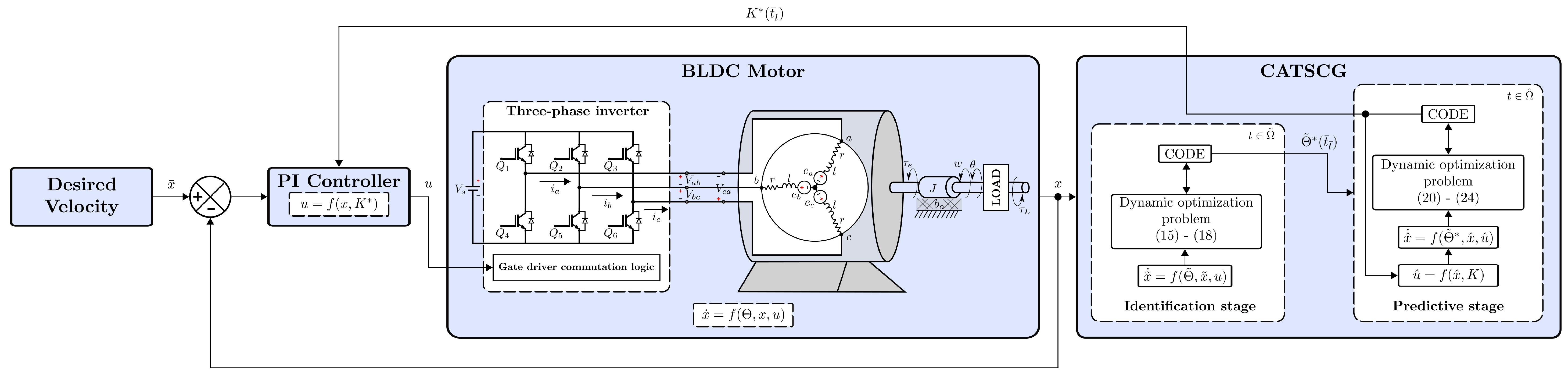
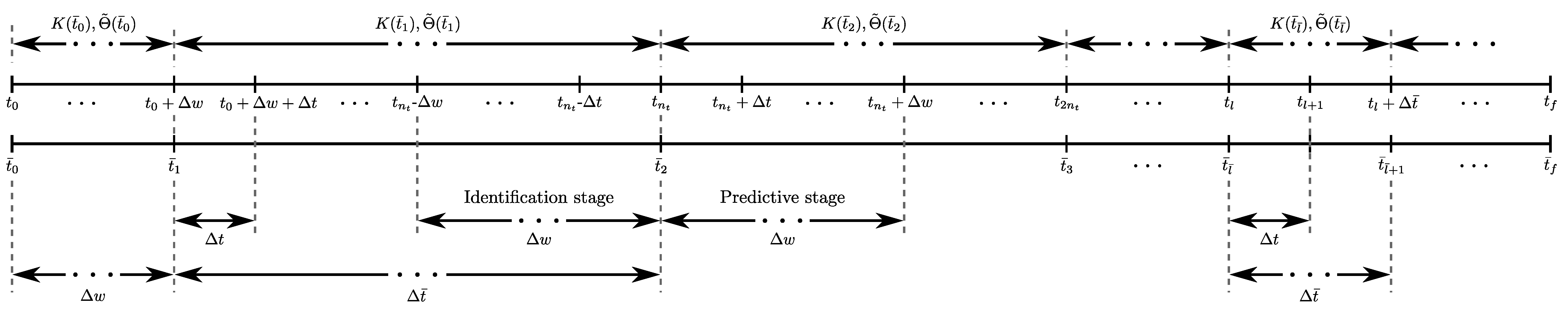
Concerning the re-optimization process in the identification and predictive stages of the CATSCG for the PI controller, it is performed by CODE every $\Delta \overline{t}=5\left(\mathrm{ms}\right)$.

The dynamic optimization problem for identification is set up using the past brushless states acquired in a backward time window of $\Delta w=50\left(\mathsf{\mu }\mathrm{s}\right)$ from the current time instant. The upper and lower bounds of the model parameters for this problem are set as ${\tilde{\Theta }}_{max}={[2\frac{b_0}{J},2\frac{k_m}{J},2\frac{k_e}{L},2\frac{R}{L},2\frac{1}{L},2\frac{1}{J},0.05]}^T$ and ${\tilde{\Theta }}_{min}={[\frac{1}{2}\frac{b_0}{J},\frac{1}{2}\frac{k_m}{J},\frac{1}{2}\frac{k_e}{L},\frac{1}{2}\frac{R}{L},\frac{1}{2}\frac{1}{L},\frac{1}{2}\frac{1}{J},0]}^T$. As can be noticed, these bounds are based on the nominal values of the system parameters as suggested in [73] to prevent the model over-fitting. In this way, the lower bounds correspond to half the value of the nominal parameters, while the upper ones correspond to double. The above rule is simple and allows to set the limits considering approximate values of the motor parameters and not necessarily the actual ones.

In the case of the predictive stage, a future horizon of $\Delta w=50\left(\mathsf{\mu }\mathrm{s}\right)$ is selected to predict the motor behavior for different sets of controller gains. For this last problem, the input voltage limits are ${\widehat{u}}_{min}=-250\left(\mathrm{V}\right)$ and ${\widehat{u}}_{max}=250\left(\mathrm{V}\right)$. For the same problem, the selected upper and lower bounds of the PI controller gains are $K_{max}={[200,200]}^T$ and $K_{min}={[0,0]}^T$. These limits were obtained by a non-exhaustive trial-and-error approach using a fixed-gain PI controller. In this, the PI gains are adjusted to observe limiting behaviors that can be considered acceptable, but not necessarily good..

In addition, the effectiveness of the CODE optimizer in the proposed adaptive tuning strategy is verified through comparisons with other alternatives provided with the same elitist online adaptation (the inclusion of an individual with the best previous knowledge). These are: the genetic algorithm (GA) described in [50], a particular case of the well-known non-dominated sorting genetic algorithm II (NSGA-II) [74] where the objective function space considers a single objective; the particle swarm optimization (PSO) with a full-connected topology and a linear-decreasing inertia weight in [75], and the variant DE/rand/1/bin of differential evolution (DE). These new variants are referred to as OGA, OPSO, and ODE.

Regarding the hyperparameters of the above optimizers, there are many approaches to set them up. For instance, in the algorithms from the works in Table 1, these parameters were tuned by hand (i.e., the best hyperparameters were selected after a series of trials with different combinations) or chosen as the most promising alternative reported in the literature. In this work, the latter approach is preferred because, in practical applications, it is important to provide the parameter setting in an easy way by using a guideline, and it can be more attractive to engineers for implementation purposes. So, the algorithm parameter settings are set based on the suggestions found in the specialized literature, as follows—crossover rate $CR=0.5$ and scaling factor $F=0.5$ for ODE and CODE [76]; crossover probability $p_c=1$, mutation probability $p_m=\frac{1}{d}$ with d as the number of design variables, distribution index ${\eta }_c=20$ in the simulated binary crossover (SBX), and distribution index ${\eta }_m=20$ in the polynomial mutation (PM) for OGA [74]; personal and global knowledge constants $C_1=2$ and $C_1=2$, and minimum and maximum value of inertia weight ${\overline{w}}_{min}=0.4$ and ${\overline{w}}_{max}=0.9$ for OPSO [77]. To produce fair comparisons, the number of objective function evaluations is the same for all optimizers, determined by the number of candidate vectors $NP=25$ and the maximum number of iterations $G_{max}=10$.

4.2. Discussion of the Results

The proposal was tested for the two operating conditions (NOC and DOC) through thirty independent runs for each of the previously described optimizers. For simplicity, the prefix ATCB (adaptive tuning for the controller in BLDC motors) refers to the adaptive tuning strategy based on any other optimizer than CODE. In this way, the alternatives compared with the proposed CATSCG are ATCB/ODE, ATCB/OGA, and ATCB/OPSO.

Each independent run was evaluated using the integral square error (ISE), a helpful performance metric to assess the transient controller response since it (more) weights the large errors [78].

Table 4. Descriptive statistical results.

Cond.	Strategy	Mean (ISE)	STD (ISE)	Min (ISE)	Max (ISE)
NOC	CATSCG	25.0690	0.5515	24.7177	26.7540
	ATCB/ODE	25.7099	0.6303	24.8184	26.5760
	ATCB/OGA	25.6657	0.6827	24.7470	26.4691
	ATCB/OPSO	26.1632	0.4290	24.8573	26.9761
DOC	CATSCG	28.2791	1.0214	27.3197	31.3868
	ATCB/ODE	28.7739	0.9620	27.2317	30.6307
	ATCB/OGA	28.8977	0.8481	27.1414	30.0556
	ATCB/OPSO	29.5448	0.6452	27.7060	30.9074

outlines the descriptive statistics over the ISE results of all runs grouped by the operating conditions. This table includes the mean, standard deviation, minimum, and maximum values of ISE for each adaptive tuning strategy, and the best results are highlighted in boldface. Based on the above values, the proposed CATSCG is the best performing alternative for NOC and DOC, and is followed by ATCB/ODE, which also utilizes DE as the optimizer. On the other hand, ATCB/OGA is not far from these two controllers, and ATCB/OPSO develops the worst results. It is important to note that all strategies have a small increase in error under DOC compared to NOC. This highlights the ability of the online optimization-based strategies to handle perturbations, uncertainties, noise, and abrupt changes in the reference.

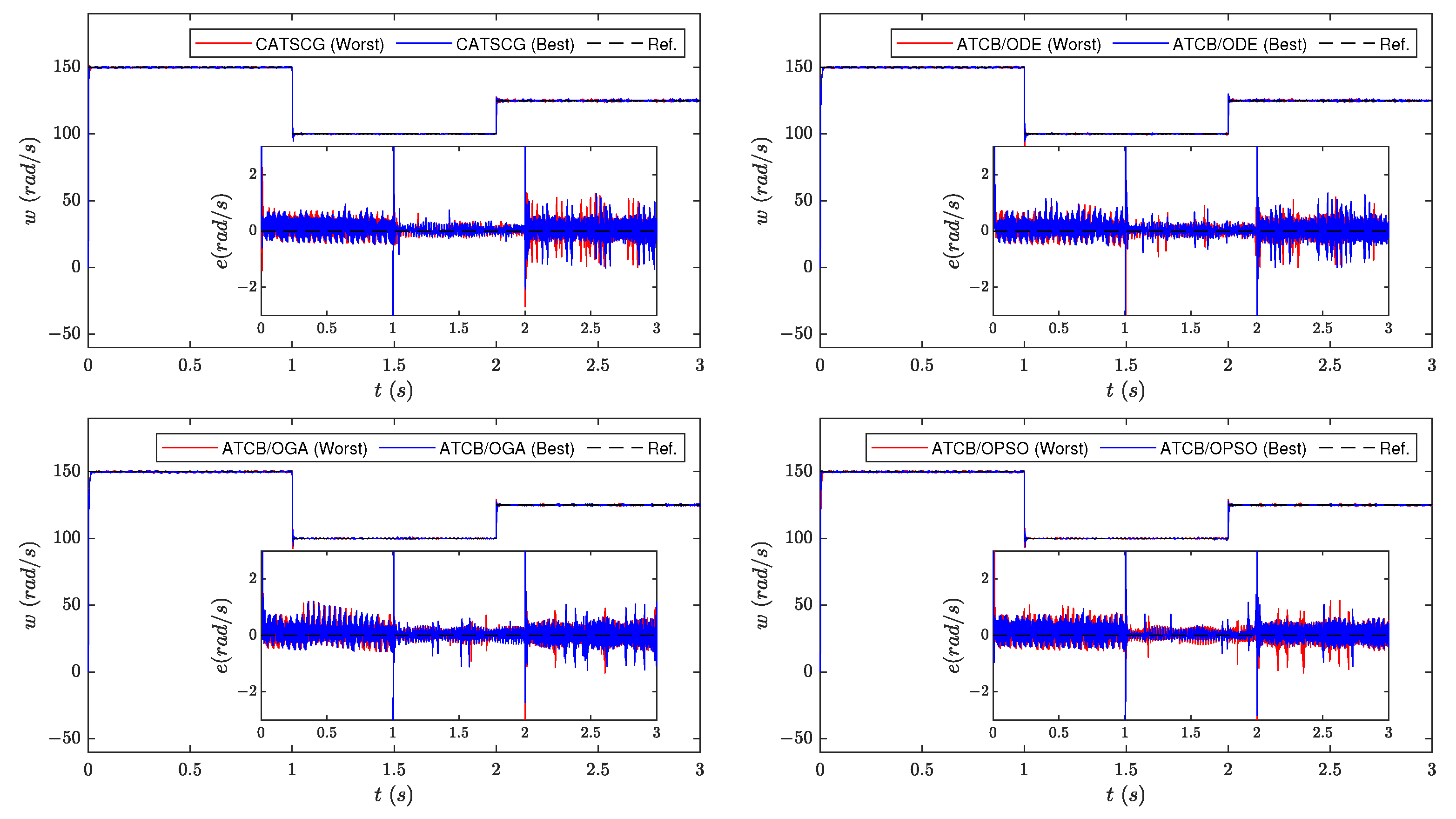
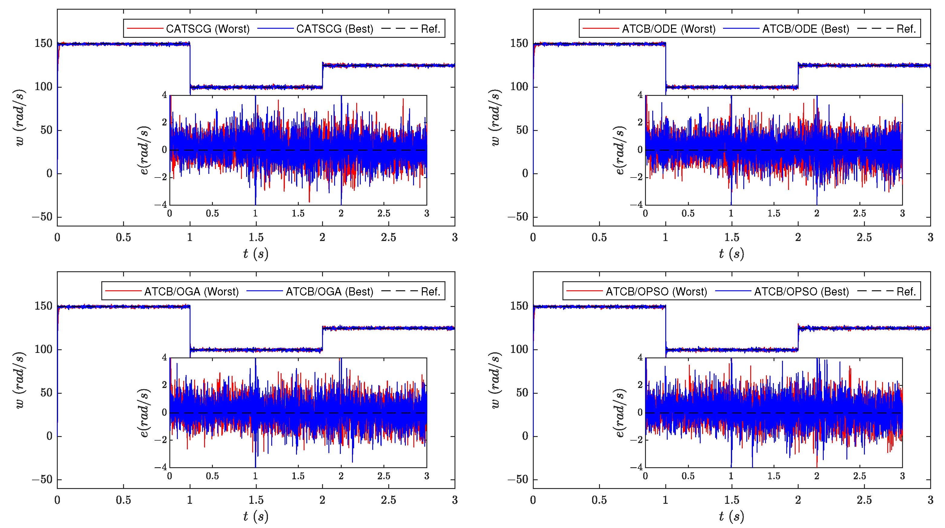
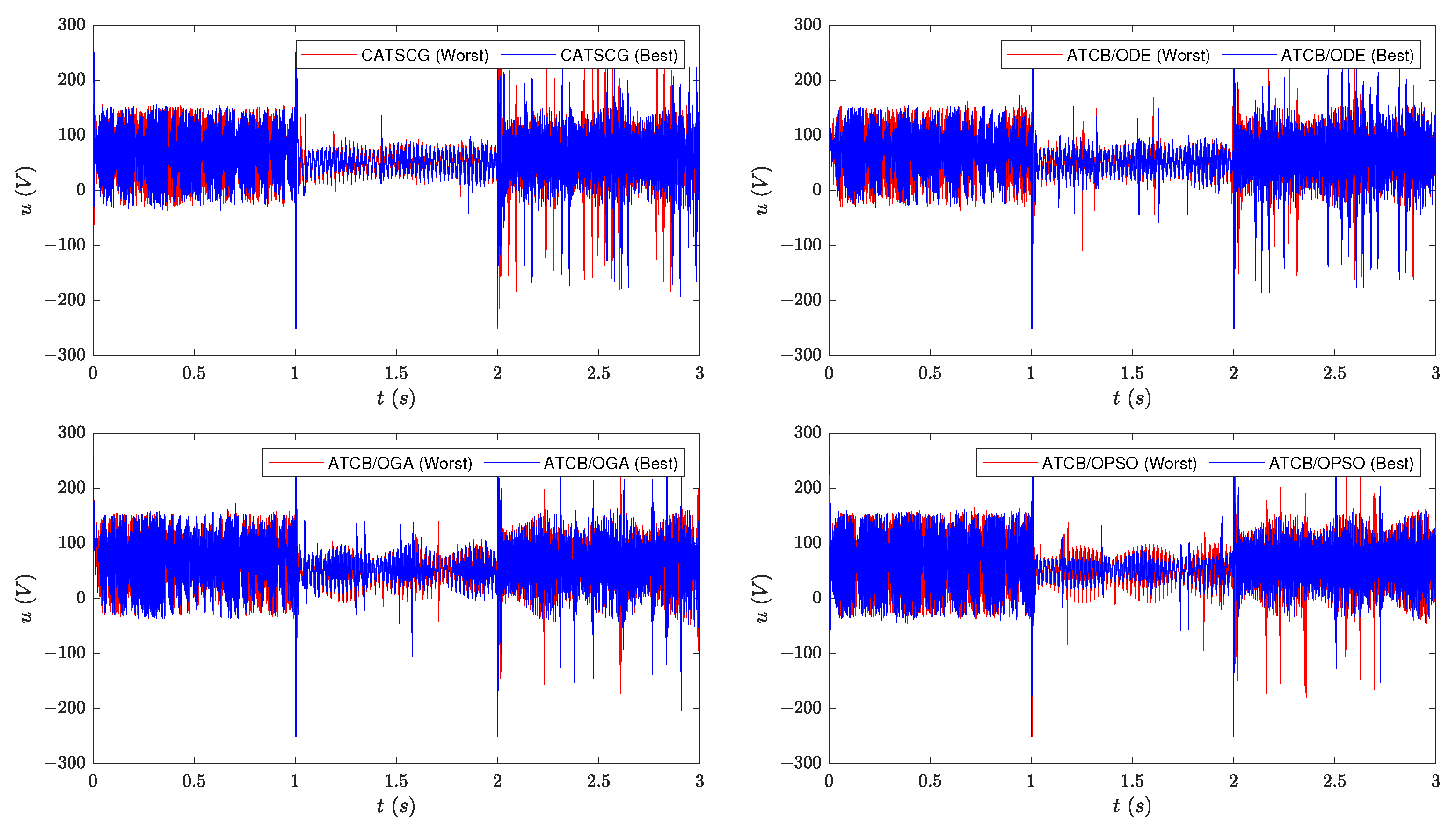
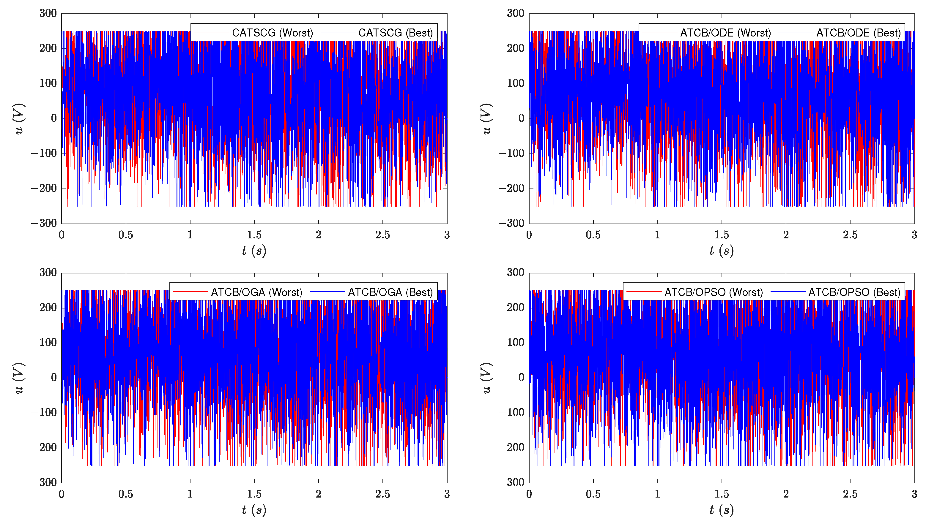
The motor output behaviors of the best and worst runs of each controller are observed in Figure 6 and Figure 7 considering NOC and DOC, respectively, while their corresponding control actions are depicted in Figure 8 and Figure 9. The inner plots of the speed figures display the evolution of the error in time.

In the speed graphs of all controller alternatives, there is no visible difference between the best and worst outputs for both NOC and DOC conditions. In the case of ATCB/OGA and ATCB/OGA, some error peaks stand out from the inner plots in comparison with the error signals of CATSCG and ATCB/ODE under DOC. In the case of ATCB/OPSO, the peak-to-peak error seems more attenuated than in the rest of the alternatives. Still, it has very high peaks and is always above the reference for both operating conditions.

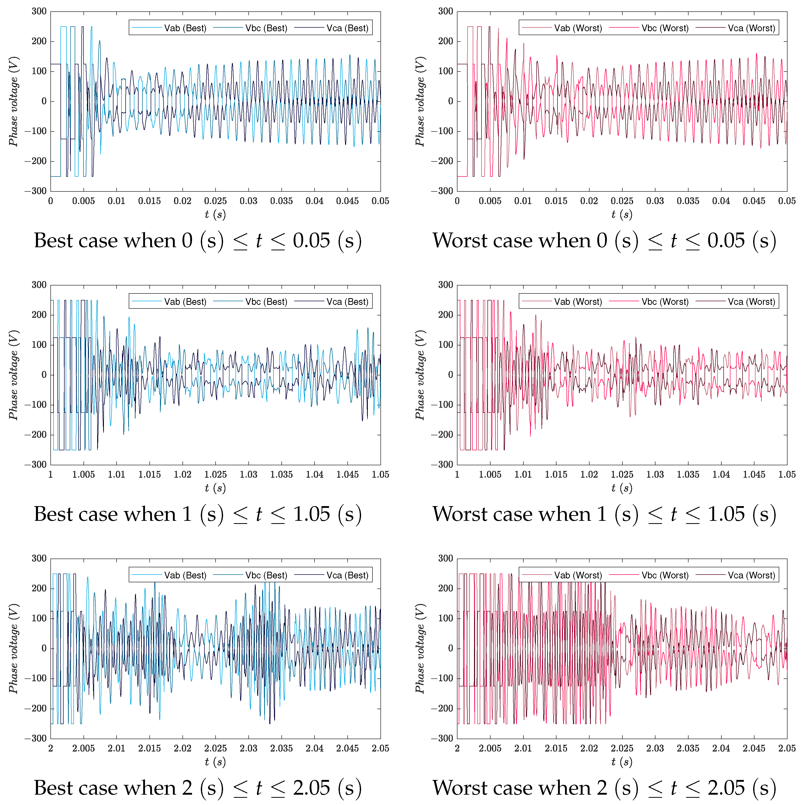
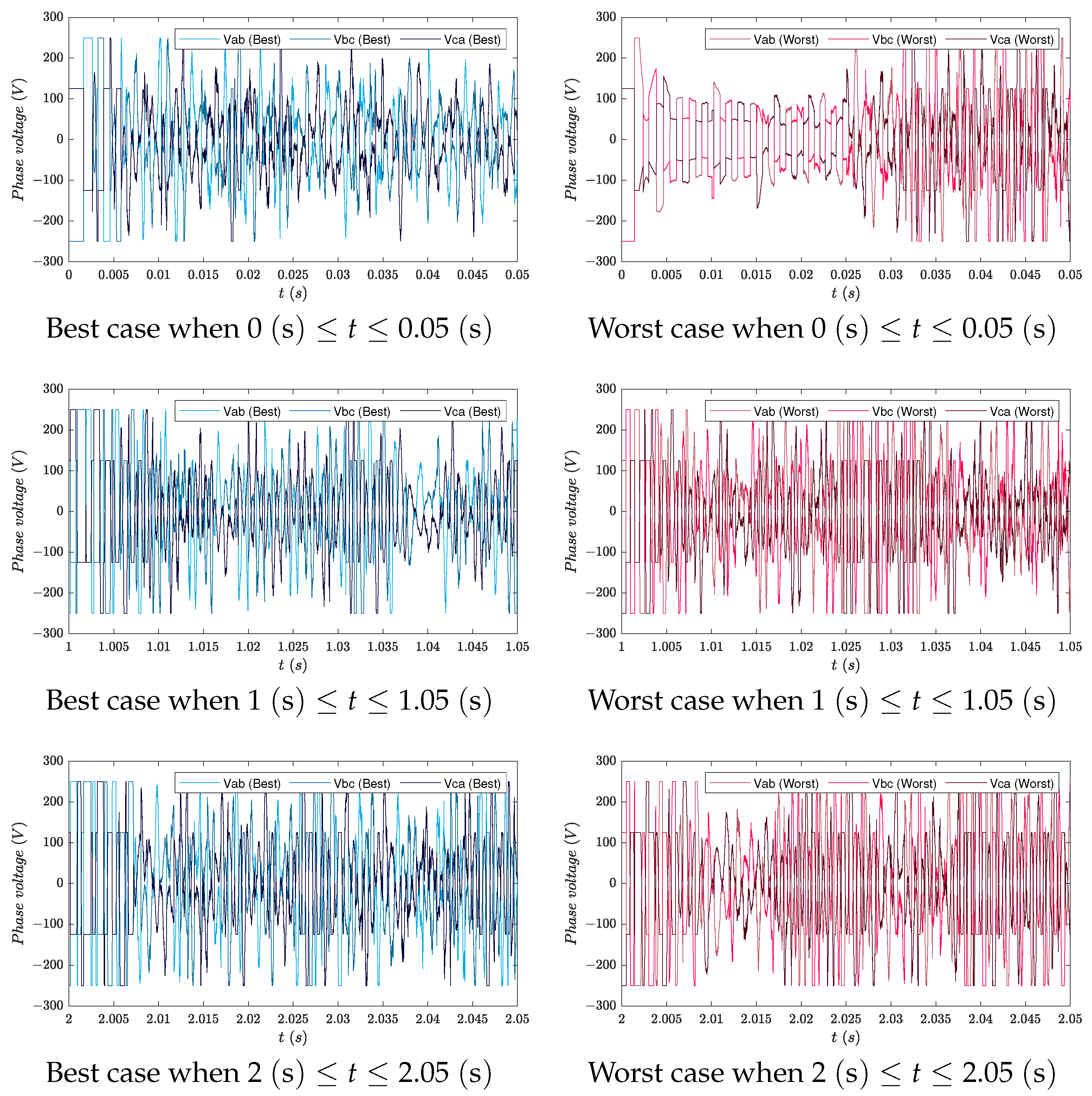
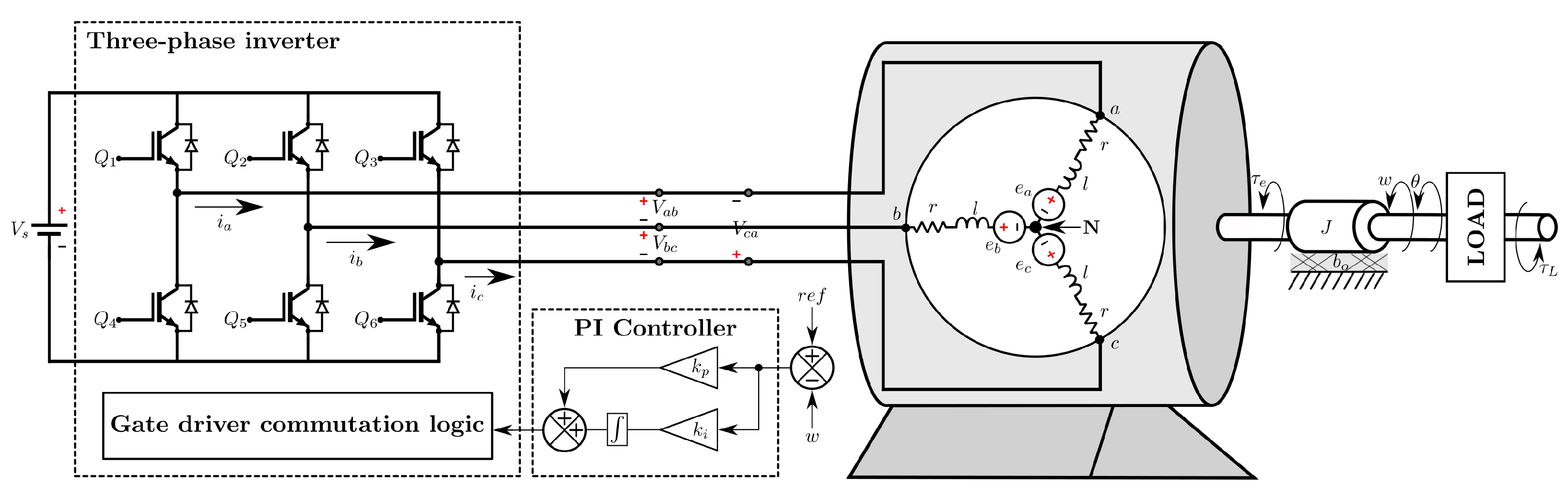
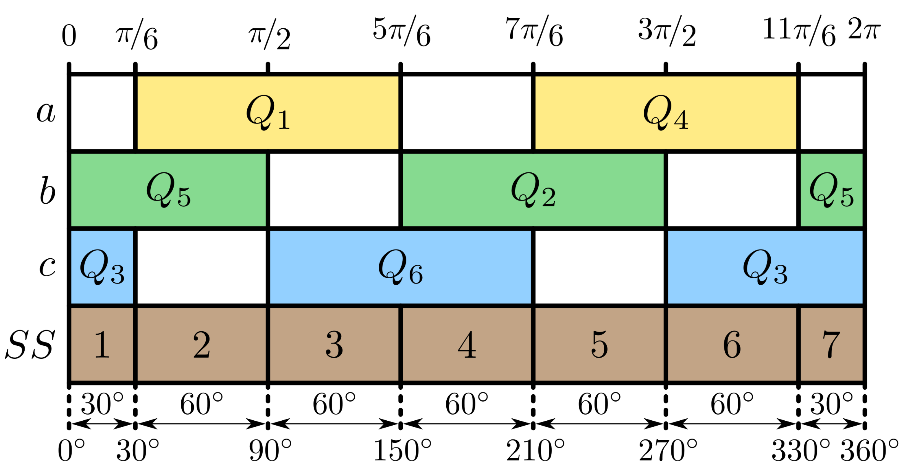
On the other hand, the control action figures reveal that control strategies require much more energy to compensate for the difficulties of DOC compared to NOC. Concerning the control action, Figure 10 and Figure 11 give examples of the operation of the coil commutation used in the brushless motor simulation. These figures show the behaviors of the phase voltages $V_{ab}$, $V_{bc}$, and $V_{ca}$ for NOC and DOC, respectively. Each figure shows a small time interval of $0.05\left(\mathrm{s}\right)$ from the $0\left(\mathrm{s}\right)$, $1\left(\mathrm{s}\right)$, and $2\left(\mathrm{s}\right)$ instants.

Returning to the error in the speed regulation task, the remarkable performances of the controllers based on DE are attributed to the suitable balance between the capacities of exploration and exploitation. In the case of ODE, the use of the elitist online adaptation only increases the exploitation ability of DE/rand/1/bin, while exploration may be compromised. In CODE, these two abilities are better balanced by using the chaotic initialization based on the Lozi map, which explains the outstanding performance of CATSCG.

In the case of OGA, the elitism improves the exploitation and is induced by sorting solutions based on fitness. However, the elitism in OGA is tougher than in ODE and CODE, as all poor-performing solutions are removed from the population at the end of each generation, i.e., only the overall fittest ones survive. In contrast, in the DE-based alternatives, selecting the elite solution is performed pairwise between an original solution and its offspring vector, which provides a gap to explore other interesting search space regions. Because of the above, there is a noticeable change in the performance of ATCB/OGA when it passes from NOC to DOC in Table 4.

On the other side, the opposite happens with OPSO, as the lack of an elitist selection mechanism favors exploration. Therefore, solutions cannot converge to a suitable solution using the available budget of objective function evaluations (this is given by $G_{max}·NP$ for each optimization process). The above implies a low control performance with ATCB/OPSO when considering NOC, which worsens under DOC.

At this point, it is essential to remember that the approximate optimizers used in this work are stochastic methods. This means that the distribution of their results does not belong to a particular shape (e.g., the normal one). So, the descriptive statistical information in Table 4 does not provide enough evidence to draw strong conclusions, although it gives a preliminary look at the behaviors of all the controllers. Therefore, the results of the experiments are evaluated in this work through two well-known non-parametric statistical tests: the pairwise Wilcoxon signed-rank test and the multi-comparative Friedman test [52].

The pairwise Wilcoxon signed-rank test compares the location of two different sets of samples. For this, a null hypothesis $H_0$ indicates no significant differences between the samples of the two sets or they share a similar location. Moreover, an alternative hypothesis $H_a$ suggests that there are noticeable differences between the samples of the two sets in three ways: the samples in the first set are to the left of those in the second (left-sided hypothesis); the samples in the first set are to the right of those in the second (right-sided hypothesis); or the samples in the first set are in a different location than those in the second (two-sided hypothesis). Then, the test outputs a p-value with the probability of accepting the $H_0$ and rejecting the $H_a$. A statistical significance $\rho$ establishes a threshold of the p-value for which the $H_a$ can be accepted (typically $5\%$).

In this study, each sets contains the ISE values of the thirty independent runs of one of the ATCB alternatives and the CATSCG for particular operating conditions. Moreover, the two-sided hypothesis is selected as the $H_a$ and the statistical significance is set as $\rho =5\%$. The results of all possible Wilcoxon tests are presented in

Table 5. Results of the pairwise Wilcoxon signed-rank test over the values of ISE for the adaptive controller tuning.

Cond.	Test	${\mathit{R}}_{+}$	${\mathit{R}}_{-}$	p-Value
NOC	CATSCG vs. ATCB/ODE	390	75	$\mathbf{0}.\mathbf{0007}\times {\mathbf{10}}^{\mathbf{0}}$
	CATSCG vs. ATCB/OGA	359	106	$\mathbf{0}.\mathbf{0081}\times {\mathbf{10}}^{\mathbf{0}}$
	CATSCG vs. ATCB/OPSO	451	14	$2.0489\times {10}^{-7}$
	ATCB/ODE vs. ATCB/OGA	222	243	$0.8393\times {10}^0$
	ATCB/ODE vs. ATCB/OPSO	377	88	$\mathbf{0}.\mathbf{0021}\times {\mathbf{10}}^{\mathbf{0}}$
	ATCB/OGA vs. ATCB/OPSO	375	90	$\mathbf{0}.\mathbf{0025}\times {\mathbf{10}}^{\mathbf{0}}$
DOC	CATSCG vs. ATCB/ODE	330	135	$\mathbf{0}.\mathbf{0449}\times {\mathbf{10}}^{\mathbf{0}}$
	CATSCG vs. ATCB/OGA	342	123	$\mathbf{0}.\mathbf{0234}\times {\mathbf{10}}^{\mathbf{0}}$
	CATSCG vs. ATCB/OPSO	434	31	$\mathbf{4}.\mathbf{4219}\times {\mathbf{10}}^{-\mathbf{6}}$
	ATCB/ODE vs. ATCB/OGA	239	226	$0.9032\times {10}^0$
	ATCB/ODE vs. ATCB/OPSO	400	65	$\mathbf{0}.\mathbf{0002}\times {\mathbf{10}}^{\mathbf{0}}$
	ATCB/OGA vs. ATCB/OPSO	423	42	$\mathbf{2}.\mathbf{0798}\times {\mathbf{10}}^{-\mathbf{5}}$

and are grouped by the type of operating conditions. In this table, the columns $R_{+}$ and $R_{-}$ are the sums of ranks calculated for the test. In this way, $R_{+}$ indicates the times that a sample of the first set outperforms a sample of the second, while $R_{-}$ indicates the contrary. These two columns are displayed to determine the location of the samples of each set and, therefore, decide the winner in boldface when p-value $\le \rho$.

Table 6. Summary of the pairwise Wilcoxon signed-rank test over the values of ISE for the adaptive controller tuning.

Strategy	Wins under NOC	Wins under DOC	Total Wins
CATSCG	3	3	6
ATCB/ODE	1	1	2
ATCB/OGA	1	1	2
ATCB/OPSO	0	0	0

summarizes the results of the Wilcoxon tests, where it is observed that the alternative in boldface, i.e., CATSCG, is the best choice since it obtained a greater number of wins, followed by ATCB/ODE and ATCB/OGA, which performed equally well, and finally by ATCB/OPSO.

Pairwise non-parametric statistical tests, such as the Wilcoxon test, are helpful to compare the samples of two different sets. However, when one wants to compare the samples of several sets as a group, multi-comparative non-parametric statistical tests are necessary [52].

The multi-comparative Friedman test compares the location of the samples of two or more sets. As in the Wilcoxon case, the Friedman test includes a null hypothesis $H_0$ to indicate no significant differences among the compared sets but adopts a unique alternative hypothesis $H_a$ that suggests the opposite. The p-value obtained with this test also refers to the probability of accepting the $H_0$. So, a statistical significance $\rho$ (often $5\%$) is required to determine when $H_a$ is valid.

In this work, the multi-comparative Friedman test, with $\rho =5\%$, was applied to the sets of ISE samples for the adaptive controller tuning and the particular operating conditions. The results of this test are displayed in

Table 7. Results of the multi-comparative Friedman test over the values of ISE for the adaptive controller tuning.

Cond.	Strategy	Rank	Statistic	p-Value
NOC	CATSCG	1.667	23.76	$2.8034\times {10}^{-5}$
	ATCB/ODE	2.667
	ATCB/OGA	2.4
	ATCB/OPSO	3.267
DOC	CATSCG	1.9	21	$1.0528\times {10}^{-4}$
	ATCB/ODE	2.467
	ATCB/OGA	2.267
	ATCB/OPSO	3.367

and, according to the p-value, there are significant differences among the behaviors of all controllers for NOC and DOC (p-value $\le \rho$ in both cases). The magnitude of those differences is observed in the statistic column, which includes the chi-squared (${\chi }^2$) statistic value of the test. In this sense, the differences in the performance of the controllers are greater in NOC than in DOC. Additionally, Table 7 shows the ranks computed with the Friedman test, indicating a particular order of the studied alternatives concerning control performance. In this way, the order from best to worst is the same for both operating conditions: (1) CATSCG, (2) ATCB/ODE, (3) ATCB/OGA, and (4) ATCB/OPSO.

Based on the multi-comparative Friedman test results, all control choices have significantly different performances from each other no matter the operating conditions. Now, it is possible to perform post hoc Friedman tests to analyze particular pairwise cases and determine which ISE sets perform better. For this, the $H_0$ and $H_a$ hypotheses are the same as in the multi-comparative Friedman test, and the statistical significance is also established as $\rho =5\%$.

Table 8. Results of the post hoc Friedman test over the values of ISE for the adaptive controller tuning.

Cond.	Test	Unadjusted	Holm	Shaffer	Bergmann	z
NOC	CATSCG vs. ATCB/ODE	$\mathbf{2}.\mathbf{6998}\times {\mathbf{10}}^{-\mathbf{3}}$	$\mathbf{1}.\mathbf{3499}\times {\mathbf{10}}^{-\mathbf{2}}$	$\mathbf{8}.\mathbf{0994}\times {\mathbf{10}}^{-\mathbf{3}}$	$\mathbf{8}.\mathbf{0994}\times {\mathbf{10}}^{-\mathbf{3}}$	−3
	CATSCG vs. ATCB/OGA	$\mathbf{2}.\mathbf{7807}\times {\mathbf{10}}^{-\mathbf{2}}$	$8.3421\times {10}^{-2}$	$8.3421\times {10}^{-2}$	$5.5614\times {10}^{-2}$	−2.2
	CATSCG vs. ATCB/OPSO	$\mathbf{1}.\mathbf{5867}\times {\mathbf{10}}^{-\mathbf{6}}$	$\mathbf{9}.\mathbf{5199}\times {\mathbf{10}}^{-\mathbf{6}}$	$\mathbf{9}.\mathbf{5199}\times {\mathbf{10}}^{-\mathbf{6}}$	$\mathbf{9}.\mathbf{5199}\times {\mathbf{10}}^{-\mathbf{6}}$	−4.8
	ATCB/ODE vs. ATCB/OGA	4.2371E-01	$4.2371\times {10}^{-1}$	$4.2371\times {10}^{-1}$	$4.2371\times {10}^{-1}$	0.8
	ATCB/ODE vs. ATCB/OPSO	$7.1861\times {10}^{-2}$	$1.4372\times {10}^{-1}$	$1.4372\times {10}^{-1}$	$7.1861\times {10}^{-2}$	−1.8
	ATCB/OGA vs. ATCB/OPSO	$\mathbf{9}.\mathbf{3224}\times {\mathbf{10}}^{-\mathbf{3}}$	$\mathbf{3}.\mathbf{7290}\times {\mathbf{10}}^{-\mathbf{2}}$	$\mathbf{2}.\mathbf{7967}\times {\mathbf{10}}^{-\mathbf{2}}$	$\mathbf{2}.\mathbf{7967}\times {\mathbf{10}}^{-\mathbf{2}}$	−2.6
DOC	CATSCG vs. ATCB/ODE	$8.9131\times {10}^{-2}$	$2.6739\times {10}^{-1}$	$2.6739\times {10}^{-1}$	$2.6739\times {10}^{-1}$	−1.7
	CATSCG vs. ATCB/OGA	$2.7133\times {10}^{-1}$	$5.4266\times {10}^{-1}$	$5.4266\times {10}^{-1}$	$2.7133\times {10}^{-1}$	−1.1
	CATSCG vs. ATCB/OPSO	$\mathbf{1}.\mathbf{0825}\times {\mathbf{10}}^{-\mathbf{5}}$	$\mathbf{6}.\mathbf{4951}\times {\mathbf{10}}^{-\mathbf{5}}$	$\mathbf{6}.\mathbf{4951}\times {\mathbf{10}}^{-\mathbf{5}}$	$\mathbf{6}.\mathbf{4951}\times {\mathbf{10}}^{-\mathbf{5}}$	−4.4
	ATCB/ODE vs. ATCB/OGA	$5.4851\times {10}^{-1}$	$5.4851\times {10}^{-1}$	$5.4851\times {10}^{-1}$	$5.4851\times {10}^{-1}$	0.6
	ATCB/ODE vs. ATCB/OPSO	$\mathbf{6}.\mathbf{9339}\times {\mathbf{10}}^{-\mathbf{3}}$	$\mathbf{2}.\mathbf{7736}\times {\mathbf{10}}^{-\mathbf{2}}$	$\mathbf{2}.\mathbf{0802}\times {\mathbf{10}}^{-\mathbf{2}}$	$\mathbf{1}.\mathbf{3868}\times {\mathbf{10}}^{-\mathbf{2}}$	−2.7
	ATCB/OGA vs. ATCB/OPSO	$\mathbf{9}.\mathbf{6685}\times {\mathbf{10}}^{-\mathbf{4}}$	$\mathbf{4}.\mathbf{8342}\times {\mathbf{10}}^{-\mathbf{3}}$	$\mathbf{2}.\mathbf{9005}\times {\mathbf{10}}^{-\mathbf{3}}$	$\mathbf{2}.\mathbf{9005}\times {\mathbf{10}}^{-\mathbf{3}}$	−3.3

shows the results of all possible post hoc Friedman tests over the sets of ISE samples for adaptive controller tuning and NOC and DOC conditions. In addition to the operating conditions and the information on the test performed, this table includes the unadjusted p-value and its Holm, Shaffer, and Bergmann corrections [52], which are highlighted in boldface when they are $\le \rho$ (i.e., when $H_a$ is accepted). The above corrected values help to compensate for errors included in the p-value calculation for post hoc tests [52]. Moreover, the test statistic, denoted by z, is shown in the same table to determine the location of each result set. In this way, a negative value of z indicates that the first alternative overcomes the second, while a positive one indicates the opposite.

Table 9. Summary of the post hoc Friedman test over the values of ISE for the adaptive controller tuning.

Strategy	Wins under NOC	Wins under DOC	Total Wins
CATSCG	9	4	13
ATCB/ODE	0	4	4
ATCB/OGA	4	4	8
ATCB/OPSO	0	0	0

summarizes the results of the above post hoc Friedman tests. According to the number of wins in this table, the choice in boldface, i.e., CATSCG, has the best performance and is followed by ATCB/OGA, ATCB/ODE, and ATCB/OPSO.

The results of the non-parametric statistical tests presented previously confirm that CATSCG is the best alternative for the speed regulation of the brushless DC motor under normal operating condition(s) (NOC) and disturbed operating condition(s) (DOC).

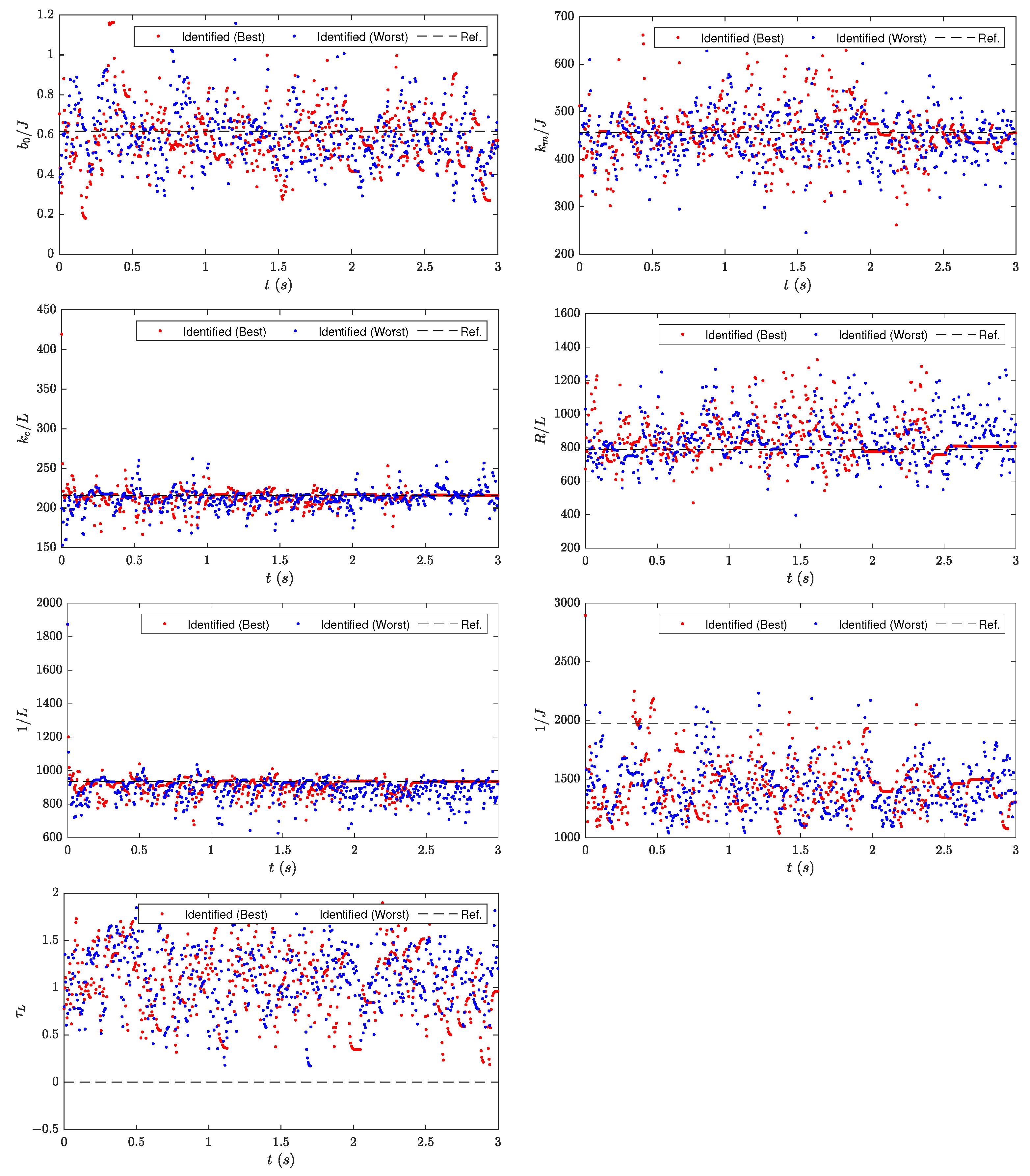
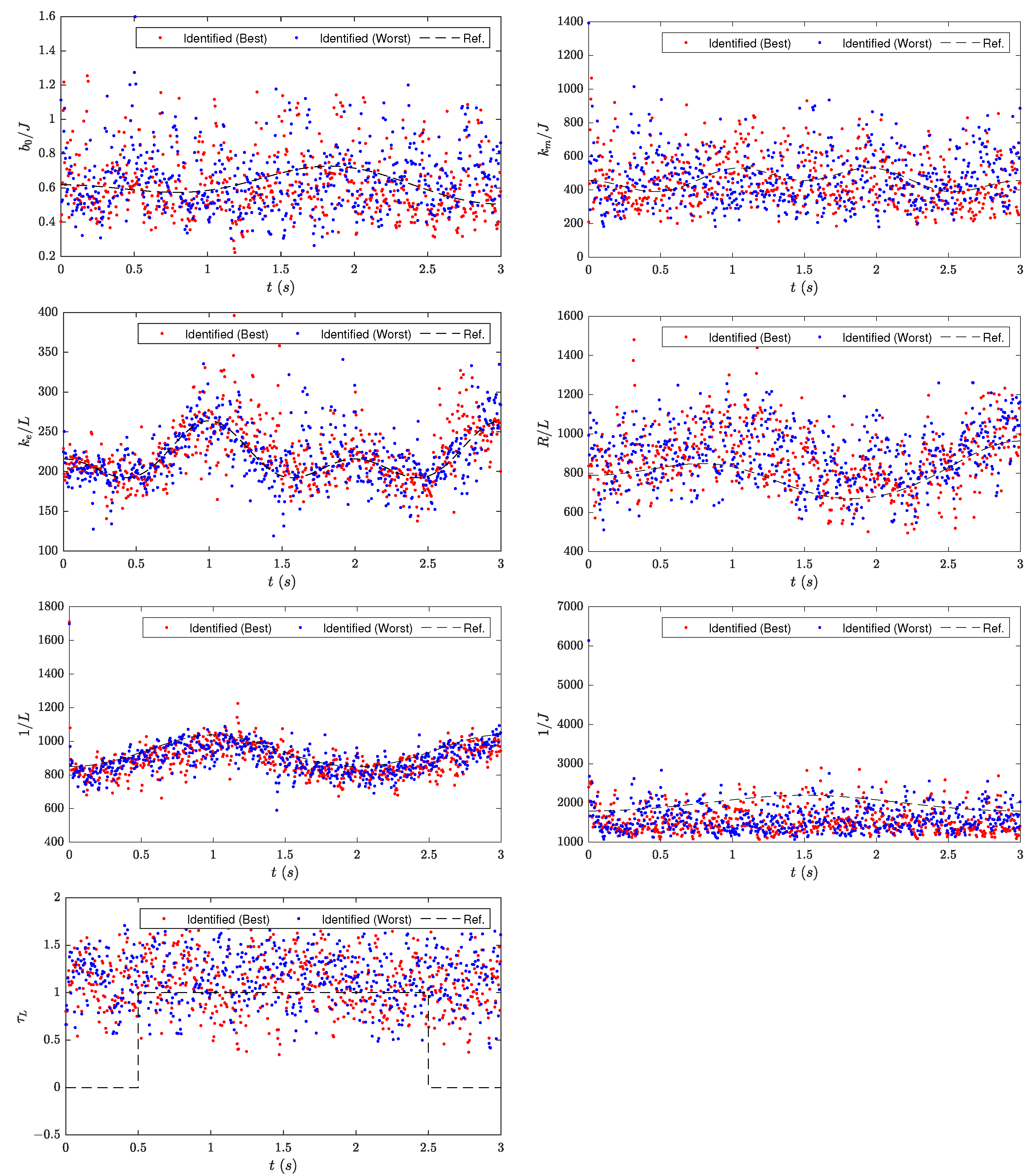
In addition to the performance of the CATSCG, it is important to know what are the behaviors of the solutions that it could obtain through online optimization. In this regard, Figure 12 and Figure 13 show the brushless motor parameters identified through CODE for the best and worst performances under NOC and DOC, respectively. These results are contrasted with the actual values of the motor parameters, which are also included in the graphs. As can be seen in these figures, the parameters identified by CATSCG are far from the actual ones. This is because the optimization problem for identification does not consider the differences between the real and identified parameters, but the difference between the acquired motor outputs and those obtained through the model simulation. In this way, there can be different combinations of parameters that, used in the model, can generalize the real behavior of the brushless motor.

An additional point to consider is the execution time of each optimization process. Currently, the average time for a run of $3\left(\mathrm{s}\right)$ is $2.5\left(\mathrm{s}\right)$ with the CATSCG. The above involved using a computer with Intel(R) Core(TM) i5-10400F CPU @ 2.90 GHz and 64.0 GB of RAM, and implementing the control strategy in C++ language through Visual Studio 2019 Community Edition. This indicates that the proposal can be tested in a future experimental stage with a laboratory prototype, but other aspects must be considered, such as the characteristics of the sensors and data acquisition devices, which also consume computational time.

5. Conclusions

This paper proposes the chaotic adaptive tuning strategy for controller gains (CATSCG). This strategy contains two sequential stages to set the control gains in the dynamic environment. The proposal is applied to the tuning of the PI controller of a BLDC motor. The main feature of the proposed CATSCG is the inclusion of a novel chaotic online differential evolution (CODE) in the identification and predictive stages.

Among the tested optimizers (ODE, OGA, and OPSO) in the adaptive controller tuning, the statistical results evidence that the use of CODE suitably balances the search capacities of exploration and exploitation of the algorithm, such that the proposed CATSCG maintains, as minimum as possible, the motor velocity error under the effects of disturbances, uncertainties, noise, and reference velocity changes. The outstanding performance of CATSCG is attributed to the use of the chaotic initialization based on the Lozi map.

The obtained results in the dynamic process indicate that the generation of the initial population through the use of the Lozi chaotic map positively impacts the performance of the differential evolution algorithm for dynamically setting the gains in the BLDC motor controller. Every time the tuning process is called, the results indicate that the algorithm performance does not increase with a random initial population.

The nonparametric statistical test confirms the reliability of the proposed CATSCG in the BLDC motor under the effects of disturbances.

Future work will involve the experimental evidence of the proposed CATSCG and the implementation of CATSCG in systems with more complex dynamics. The primary consideration of using CATSCG in complex dynamics is that the optimization processes in the CATSCG must be computed in—at most—the time interval between two tuning processes ($\Delta \overline{t}s$) for real-time implementations.

The initialization of the CODE is an important factor in the convergence time and the precision of the CATSCG. Therefore, future work will involve incorporating a lookup table for the initial parameters according to the operative conditions and analyzing the effects of uncertainties and disturbances in the closed-loop system.

References

1. Wang, Z.; Zou, L.; Su, X.; Luo, G.; Li, R.; Huang, Y. Hybrid force/position control in workspace of robotic manipulator in uncertain environments based on adaptive fuzzy control. Robot. Auton. Syst. 2021, 145, 103870. [Google Scholar] [CrossRef]
2. Mohanraj, D.; Aruldavid, R.; Verma, R.; Sathyasekar, K.; Barnawi, A.B.; Chokkalingam, B.; Mihet-Popa, L. A Review of BLDC Motor: State of Art, Advanced Control Techniques, and Applications. IEEE Access 2022, 10, 54833–54869. [Google Scholar] [CrossRef]
3. Li, H.; Li, W.; Ren, H. Fault-Tolerant Inverter for High-Speed Low-Inductance BLDC Drives in Aerospace Applications. IEEE Trans. Power Electron. 2017, 32, 2452–2463. [Google Scholar] [CrossRef]
4. Naseri, F.; Farjah, E.; Ghanbari, T. An Efficient Regenerative Braking System Based on Battery/Supercapacitor for Electric, Hybrid, and Plug-In Hybrid Electric Vehicles With BLDC Motor. IEEE Trans. Veh. Technol. 2017, 66, 3724–3738. [Google Scholar] [CrossRef]
5. Liu, W.; Zhou, Q.; Sheng, Q.; Kong, Q. Brushless DC motor control system based on submarine hybrid transmission technology. In Proceedings of the 2013 OCEANS, San Diego, CA, USA, 23–27 September 2013; pp. 1–4. [Google Scholar]
6. Chen, Z.; Chen, Z.; Liu, X. A 2MW 6-phase BLDC generator developed from a PM synchronous generator for wind energy application. In Proceedings of the 2014 IEEE International Conference on Industrial Technology (ICIT), Busan, Korea, 26 February–1 March 2014; pp. 110–114. [Google Scholar]
7. Kumar, R.; Singh, B. BLDC motor driven water pump fed by solar photovoltaic array using boost converter. In Proceedings of the 2015 Annual IEEE India Conference (INDICON), New Delhi, India, 17–20 December 2015; pp. 1–6. [Google Scholar]
8. Chiasson, J. Modeling and High-Performance Control of Electric Machines; Wiley: Hoboken, NJ, USA, 2005. [Google Scholar]
9. Kim, T.H.; Ehsani, M. Sensorless control of the BLDC motors from near-zero to high speeds. IEEE Trans. Power Electron. 2004, 19, 1635–1645. [Google Scholar] [CrossRef]
10. Merugumalla, M.K.; Navuri, P.K. Inertia Weight Strategies in PSO for BLDC Motor Drive Control. In Microelectronics, Electromagnetics and Telecommunications; Panda, G., Satapathy, S.C., Biswal, B., Bansal, R., Eds.; Springer: Singapore, 2019; pp. 475–484. [Google Scholar]
11. Krishnan, R. Electric Motor Drives: Modeling, Analysis, and Control; Prentice Hall: New Jersey, NJ, USA, 2001; Volume 626. [Google Scholar]
12. Joseph, S.B.; Dada, E.G.; Abidemi, A.; Oyewola, D.O.; Khammas, B.M. Metaheuristic algorithms for PID controller parameters tuning: Review, approaches and open problems. Heliyon 2022, 8, e09399. [Google Scholar] [CrossRef]
13. Multi-objective meta-heuristic optimization in intelligent control: A survey on the controller tuning problem. Appl. Soft Comput. 2020, 93, 106342. [CrossRef]
14. Astrom, K.J.; Hagglund, T. Advanced PID Control; ISA-The Instrumentation, Systems and Automation Society: Research Triangl, NC, USA, 2006. [Google Scholar]
15. Marques, T.; Reynoso-Meza, G. Applications of multi-objective optimisation for PID-like controller tuning: A 2015–2019 review and analysis. IFAC-PapersOnLine 2020, 53, 7933–7940. [Google Scholar] [CrossRef]
16. Villarreal-Cervantes, M.G.; Alvarez-Gallegos, J. Off-line PID control tuning for a planar parallel robot using DE variants. Expert Syst. Appl. 2016, 64, 444–454. [Google Scholar] [CrossRef]
17. Villarreal-Cervantes, M.G.; Rodríguez-Molina, A.; García-Mendoza, C.V.; Peñaloza-Mejía, O.; Sepúlveda-Cervantes, G. Multi-Objective On-Line Optimization Approach for the DC Motor Controller Tuning Using Differential Evolution. IEEE Access 2017, 5, 20393–20407. [Google Scholar] [CrossRef]
18. Mendoza, M.; Zavala-Río, A.; Santibáñez, V.; Reyes, F. A generalised PID-type control scheme with simple tuning for the global regulation of robot manipulators with constrained inputs. Int. J. Control 2015, 88, 1995–2012. [Google Scholar] [CrossRef]
19. Hernández-Guzmán, V.M.; Santibáñez, V.; Silva-Ortigoza, R. A New Tuning Procedure for PID Control of Rigid Robots. Adv. Robot. 2008, 22, 1007–1023. [Google Scholar] [CrossRef]
20. Luyben, W.L.; Luyben, M.L. Essentials of Process Control; McGraw-Hill: New York, NY, USA, 1997. [Google Scholar]
21. Joseph, E.; Olaiya, O. Cohen-Coon PID Tuning Method: A Better Option to Ziegler Nichols-Pid Tuning Method. Comput. Eng. Intell. Syst. 2018, 9, 33–37. [Google Scholar]
22. Åström, K.; Hägglund, T. Revisiting the Ziegler–Nichols step response method for PID control. J. Process Control 2004, 14, 635–650. [Google Scholar] [CrossRef]
23. Marlin, T. Process Control; McGraw-Hill: New York, NY, USA, 2000. [Google Scholar]
24. Somefun, O.A.; Akingbade, K.; Dahunsi, F. The dilemma of PID tuning. Annu. Rev. Control 2021, 52, 65–74. [Google Scholar] [CrossRef]
25. de Silva, C.W. Intelligent Control. In Computational Complexity: Theory, Techniques, and Applications; Springer: New York, NY, USA, 2012; pp. 1619–1641. [Google Scholar]
26. Roveda, L.; Forgione, M.; Piga, D. Robot control parameters auto-tuning in trajectory tracking applications. Control Eng. Pract. 2020, 101, 104488. [Google Scholar] [CrossRef]
27. Loris, R.; Maskani, J.; Franceschi, P.; Abdi, A.; Braghin, F.; Molinari Tosatti, L.; Pedrocchi, N. Model-Based Reinforcement Learning Variable Impedance Control for Human-Robot Collaboration. J. Intell. Robot. Syst. 2020, 100, 417–433. [Google Scholar]
28. Talbi, E.G. Metaheuristics: From Design to Implementation; Wiley Publishing: Hoboken, NJ, USA, 2009. [Google Scholar]
29. Wang, L. PID Control System Design and Automatic Tuning Using Matlab/Simulink; John Wiley Sons: Hoboken, NJ, USA, 2020. [Google Scholar]
30. Caponio, A.; Cascella, G.L.; Neri, F.; Salvatore, N.; Sumner, M. A Fast Adaptive Memetic Algorithm for Online and Offline Control Design of PMSM Drives. IEEE Trans. Syst. Man Cybern. Part B (Cybern.) 2007, 37, 28–41. [Google Scholar] [CrossRef]
31. García, M.; Ponce, P.; Soriano, L.A.; Molina, A.; MacCleery, B.; Romero, D. Lifetime Improved in Power Electronics for BLDC Drives using Fuzzy Logic and PSO. IFAC-Pap. 2019, 52, 2372–2377. [Google Scholar] [CrossRef]
32. Jigang, H.; Hui, F.; Jie, W. A PI controller optimized with modified differential evolution algorithm for speed control of BLDC motor. Automatika 2019, 60, 135–148. [Google Scholar] [CrossRef]
33. Premkumar, K.; Manikandan, B. Speed control of Brushless DC motor using bat algorithm optimized Adaptive Neuro-Fuzzy Inference System. Appl. Soft Comput. 2015, 32, 403–419. [Google Scholar] [CrossRef]
34. Premkumar, K.; Manikandan, B.V.; Kumar, C.A. Antlion Algorithm Optimized Fuzzy PID Supervised On-line Recurrent Fuzzy Neural Network Based Controller for Brushless DC Motor. Electr. Power Components Syst. 2017, 45, 2304–2317. [Google Scholar] [CrossRef]
35. Xie, W.; Wang, J.S.; Wang, H.B. PI controller of speed regulation of brushless DC motor based on particle swarm optimization algorithm with improved inertia weights. Math. Probl. Eng. 2019, 2019, 2671792. [Google Scholar] [CrossRef]
36. Sivarani, T.; Jawhar, S.J.; Kumar, C.A. Novel bacterial foraging-based ANFIS for speed control of matrix converter-fed industrial BLDC motors operated under low speed and high torque. Neural Comput. Appl. 2018, 29, 1411–1434. [Google Scholar] [CrossRef]
37. Hu, H.; Wang, T.; Zhao, S.; Wang, C. Speed control of brushless direct current motor using a genetic algorithm–optimized fuzzy proportional integral differential controller. Adv. Mech. Eng. 2019, 11, 1687814019890199. [Google Scholar] [CrossRef]
38. Potnuru, D.; Alice Mary, K.; Sai Babu, C. Experimental implementation of Flower Pollination Algorithm for speed controller of a BLDC motor. Ain Shams Eng. J. 2019, 10, 287–295. [Google Scholar] [CrossRef]
39. Potnuru, D.; Tummala, A.S.L.V. Implementation of Grasshopper Optimization Algorithm for Controlling a BLDC Motor Drive. In Soft Computing in Data Analytics; Nayak, J., Abraham, A., Krishna, B.M., Chandra Sekhar, G.T., Das, A.K., Eds.; Springer: Singapore, 2019; pp. 369–376. [Google Scholar]
40. Premkumar, K.; Manikandan, B. Bat algorithm optimized fuzzy PD based speed controller for brushless direct current motor. Eng. Sci. Technol. Int. J. 2016, 19, 818–840. [Google Scholar] [CrossRef] [Green Version]
41. Vanchinathan, K.; Valluvan, K. A metaheuristic optimization approach for tuning of fractional-order PID controller for speed control of sensorless BLDC motor. J. Circuits, Syst. Comput. 2018, 27, 1850123. [Google Scholar] [CrossRef]
42. Yigit, T.; Celik, H. Speed controlling of the PEM fuel cell powered BLDC motor with FOPI optimized by MSA. Int. J. Hydrog. Energy 2020, 45, 35097–35107. [Google Scholar] [CrossRef]
43. Demirtas, M. Off-line tuning of a PI speed controller for a permanent magnet brushless DC motor using DSP. Energy Convers. Manag. 2011, 52, 264–273. [Google Scholar] [CrossRef]
44. Ibrahim, H.; Hassan, F.; Shomer, A.O. Optimal PID control of a brushless DC motor using PSO and BF techniques. Ain Shams Eng. J. 2014, 5, 391–398. [Google Scholar] [CrossRef] [Green Version]
45. Prathibanandhi, K.; Yaashuwanth, C.; Basha, A.R. Improved torque performance in BLDC-motor-drive through Jaya optimization implemented on Xilinx platform. Microprocess. Microsyst. 2021, 81, 103681. [Google Scholar] [CrossRef]
46. Premkumar, K.; Manikandan, B. GA-PSO optimized online ANFIS based speed controller for Brushless DC motor. J. Intell. Fuzzy Syst. 2015, 28, 2839–2850. [Google Scholar] [CrossRef]
47. Kommula, B.N.; Kota, V.R. Direct instantaneous torque control of Brushless DC motor using firefly Algorithm based fractional order PID controller. J. King Saud Univ.-Eng. Sci. 2020, 32, 133–140. [Google Scholar] [CrossRef]
48. Serrano-Pérez, O.; Villarreal-Cervantes, M.G.; Rodríguez-Molina, A.; Serrano-Pérez, J. Offline robust tuning of the motion control for omnidirectional mobile robots. Appl. Soft Comput. 2021, 110, 107648. [Google Scholar] [CrossRef]
49. Zelinka, I.; Diep, Q.B.; Snášel, V.; Das, S.; Innocenti, G.; Tesi, A.; Schoen, F.; Kuznetsov, N.V. Impact of chaotic dynamics on the performance of metaheuristic optimization algorithms: An experimental analysis. Inf. Sci. 2021, 587, 692–719. [Google Scholar] [CrossRef]
50. Rodríguez-Molina, A.; Villarreal-Cervantes, M.G.; Álvarez Gallegos, J.; Aldape-Pérez, M. Bio-inspired adaptive control strategy for the highly efficient speed regulation of the DC motor under parametric uncertainty. Appl. Soft Comput. 2019, 75, 29–45. [Google Scholar] [CrossRef]
51. Rodríguez-Molina, A.; Villarreal-Cervantes, M.G.; Aldape-Pérez, M. An adaptive control study for the DC motor using meta-heuristic algorithms. Soft Comput. 2019, 23, 889–906. [Google Scholar] [CrossRef]
52. Derrac, J.; García, S.; Molina, D.; Herrera, F. A practical tutorial on the use of nonparametric statistical tests as a methodology for comparing evolutionary and swarm intelligence algorithms. Swarm Evol. Comput. 2011, 1, 3–18. [Google Scholar] [CrossRef]
53. Shahid, A.A.; Piga, D.; Braghin, F.; Roveda, L. Continuous control actions learning and adaptation for robotic manipulation through reinforcement learning. Auton. Robot. 2022, 46, 483–498. [Google Scholar] [CrossRef]
54. Betts, J.T. Practical Methods for Optimal Control and Estimation Using Nonlinear Programming, 2nd ed.; Advances in Design and Control; SIAM: Philadelpia, PA, USA, 2010. [Google Scholar]
55. Hao, Q.; Zenghao, L.; Peng, S.; Xinguo, L. Backward numerical integration method for nonlinear system. In Proceedings of the 2017 IEEE International Conference on Signal Processing, Communications and Computing (ICSPCC), Xiamen, China, 22–25 October 2017; pp. 1–4. [Google Scholar]
56. Deng, W.; Liu, H.; Xu, J.; Zhao, H.; Song, Y. An Improved Quantum-Inspired Differential Evolution Algorithm for Deep Belief Network. IEEE Trans. Instrum. Meas. 2020, 69, 7319–7327. [Google Scholar] [CrossRef]
57. Singh, D.; Kumar, V.; Vaishali; Kaur, M. Classification of COVID-19 patients from chest CT images using multi-objective differential evolution–based convolutional neural networks. Eur. J. Clin. Microbiol. Infect. Dis. 2020, 39, 1379–1389. [Google Scholar] [CrossRef]
58. Lee, C.Y.; Hung, C.H. Feature Ranking and Differential Evolution for Feature Selection in Brushless DC Motor Fault Diagnosis. Symmetry 2021, 13, 1291. [Google Scholar] [CrossRef]
59. Storn, R.; Price, K. Differential Evolution – A Simple and Efficient Heuristic for global Optimization over Continuous Spaces. J. Glob. Optim. 1997, 11, 341–359. [Google Scholar] [CrossRef]
60. Kenneth, V. Price. An introduction to differential evolution. In New Ideas in Optimization; McGraw-Hill: London, UK, 1999; pp. 79–108. [Google Scholar]
61. Deb, K. An efficient constraint handling method for genetic algorithms. Comput. Methods Appl. Mech. Eng. 2000, 186, 311–338. [Google Scholar] [CrossRef]
62. Guzmán-Gaspar, J.Y.; Mezura-Montes, E. Robust Optimization Over Time with Differential Evolution using an Average Time Approach. In Proceedings of the 2019 IEEE Congress on Evolutionary Computation (CEC), Wellington, New Zealand, 10–13 June 2019; pp. 1548–1555. [Google Scholar]
63. Zhabitskaya, E.; Zhabitsky, M. Asynchronous Differential Evolution. In Mathematical Modeling and Computational Science; Adam, G., Buša, J., Hnatič, M., Eds.; Springer: Berlin/Heidelberg, Germany, 2012; pp. 328–333. [Google Scholar]
64. Yang, S.H.; Natarajan, U. Multi-objective optimization of cutting parameters in turning process using differential evolution and non-dominated sorting genetic algorithm-II approaches. Int. J. Adv. Manuf. Technol. 2010, 49, 773–784. [Google Scholar] [CrossRef]
65. Peng, W.; Huang, M. A critical chain project scheduling method based on a differential evolution algorithm. Int. J. Prod. Res. 2014, 52, 3940–3949. [Google Scholar] [CrossRef]
66. Peng, X.; Gao, X.; Yang, S. Environment identification-based memory scheme for estimation of distribution algorithms in dynamic environments. Soft Comput. 2011, 15, 311–326. [Google Scholar] [CrossRef] [Green Version]
67. Lozi, R. Un attracteur étrange (?) du type attracteur de Hénon. J. Phys. Colloq. 1978, 39, C5–C9. [Google Scholar] [CrossRef]
68. Araujo, E.; dos, S. Coelho, L. Particle swarm approaches using Lozi map chaotic sequences to fuzzy modelling of an experimental thermal-vacuum system. Appl. Soft Comput. 2008, 8, 1354–1364. [Google Scholar] [CrossRef]
69. Senkerik, R.; Pluhacek, M.; Viktorin, A.; Kadavy, T.; Oplatkova, Z.K. Randomization of Individuals Selection in Differential Evolution. In Recent Advances in Soft Computing; Matoušek, R., Ed.; Springer International Publishing: Cham, Switzerland, 2019; pp. 180–191. [Google Scholar]
70. Eldrandaly, K.A.; Abdel-Basset, M.; Abdel-Fatah, L. PTZ-Surveillance coverage based on artificial intelligence for smart cities. Int. J. Inf. Manag. 2019, 49, 520–532. [Google Scholar] [CrossRef]
71. Li, H.; Li, K.; Chen, M.; Bao, B. Coexisting Infinite Orbits in an Area-Preserving Lozi Map. Entropy 2020, 22, 1119. [Google Scholar] [CrossRef] [PubMed]
72. Nicholl, M.J.; Wheatcraft, S.W.; Tyler, S.W.; Berkowitz, B. Is Old Faithful a strange attractor? J. Geophys. Res. Solid Earth 1994, 99, 4495–4503. [Google Scholar] [CrossRef]
73. Rodríguez-Molina, A.; Villarreal-Cervantes, M.G.; Aldape-Pérez, M. Indirect adaptive control using the novel online hypervolume-based differential evolution for the four-bar mechanism. Mechatronics 2020, 69, 102384. [Google Scholar] [CrossRef]
74. Deb, K.; Pratap, A.; Agarwal, S.; Meyarivan, T. A fast and elitist multiobjective genetic algorithm: NSGA-II. IEEE Trans. Evol. Comput. 2002, 6, 182–197. [Google Scholar] [CrossRef] [Green Version]
75. Shi, Y.; Eberhart, R. Empirical study of particle swarm optimization. In Proceedings of the 1999 Congress on Evolutionary Computation-CEC99 (Cat. No. 99TH8406), Washington, DC, USA, 6–9 July 1999; Volume 3, pp. 1945–1950. [Google Scholar]
76. Mezura-Montes, E.; Velázquez-Reyes, J.; Coello Coello, C.A. A Comparative Study of Differential Evolution Variants for Global Optimization. In Proceedings of the 8th Annual Conference on Genetic and Evolutionary Computation, Seattle, WA, USA, 8–12 July 2006; Association for Computing Machinery: New York, NY, USA, 2006; pp. 485–492. [Google Scholar]
77. Xin, J.; Chen, G.; Hai, Y. A particle swarm optimizer with multi-stage linearly-decreasing inertia weight. In Proceedings of the 2009 International Joint Conference on Computational Sciences and Optimization, Sanya, China, 24–26 April 2009; Volume 1, pp. 505–508. [Google Scholar]
78. Linkens, D.A.; Nie, J. Constructing rule-bases for multivariable fuzzy control by self-learning Part 2. Rule-base formation and blood pressure control application. Int. J. Syst. Sci. 1993, 24, 129–157. [Google Scholar] [CrossRef]
Figure 1. Three-phase motor diagram.
Mathematics 10 01977 g001
Figure 2. Switching sequence (SS) at each point of the inverter.
Mathematics 10 01977 g002
Figure 3. Schematic diagram of the proposed chaotic adaptive tuning strategy for controller gains in the BLDC motor.
Mathematics 10 01977 g003
Figure 4. Time horizon of the proposed chaotic adaptive tuning strategy for controller gains in the BLDC motor.
Mathematics 10 01977 g004
Figure 5. Lozi chaotic map with a = 1.7 , b = 0.5 , z 1 ( 0 ) = 0 , and z 2 ( 0 ) = 0 after 10,000 iterations.
Mathematics 10 01977 g005
Figure 6. Speed output for the best and worst runs of the adaptive controller tuning, considering NOC.
Mathematics 10 01977 g006
Figure 7. Speed output for the best and worst runs of the adaptive controller tuning, considering DOC.
Mathematics 10 01977 g007
Figure 8. Control action for the best and worst runs of the adaptive controller tuning, considering NOC.
Mathematics 10 01977 g008
Figure 9. Control action for the best and worst runs of the adaptive controller tuning, considering DOC.
Mathematics 10 01977 g009
Figure 10. Phase voltages in the motor obtained with the best and worst runs of CATSCG, considering NOC.
Mathematics 10 01977 g010
Figure 11. Phase voltages in the motor obtained with the best and worst runs of CATSCG, considering DOC.
Mathematics 10 01977 g011
Figure 12. Identified motor parameters for the best and worst runs of CATSCG considering NOC.
Mathematics 10 01977 g012
Figure 13. Identified motor parameters for the best and worst runs of CATSCG considering DOC.
Mathematics 10 01977 g013