
Holistic Fault Detection and Diagnosis System in Imbalanced, Scarce, Multi-Domain (ISMD) Data Setting for Component-Level Prognostics and Health Management (PHM)


Abstract
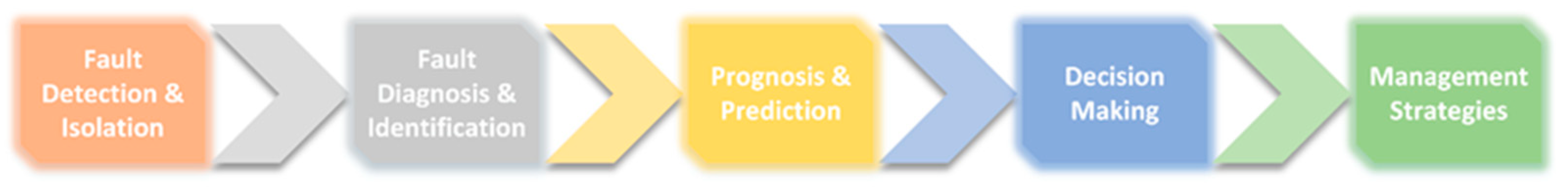
:1. Introduction
2. Materials and Methods
2.1. Experimental Test Bench
2.2. Architecture of the Proposed Methodology
- Data analysis;
- Domain knowledge transfer;
- Data splitting and classification.
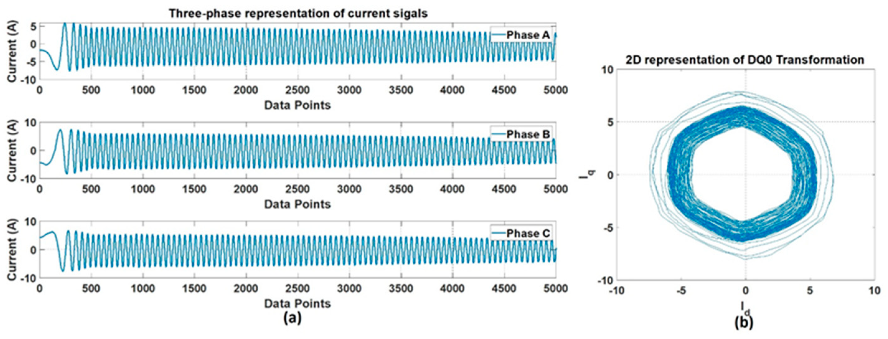
2.2.1. Data Analysis
Data Acquisition
Data Preprocessing
Signal Processing and Data Dimension Conversion
Original ISMD Data
2.2.2. Domain Knowledge Transfer
2.2.3. Data Splitting and Classification
3. Results and Discussion
3.1. Domain Knowledge Transfer for ISMD Data/Data Generation
3.2. Fault Classification
4. Conclusions
Funding
Institutional Review Board Statement
Informed Consent Statement
Acknowledgments
Conflicts of Interest
References
- Lee, J.; Wu, F.; Zhao, W.; Ghaffari, M.; Liao, L.; Siegel, D. Prognostics and Health Management Design for Rotary Machinery Systems—Reviews, Methodology and Applications. Mech. Syst. Signal Process. 2014, 42, 314–334. [Google Scholar] [CrossRef]
- Lall, P.; Lowe, R.; Goebel, K. Prognostics and Health Monitoring of Electronic Systems. In Proceedings of the 2011 12th Interantional Conference on Thermal, Mechanical & Multi-Physics Simulation and Experiments in Microelectronics and Microsystems, Linz, Austria, 18–20 April 2011. [Google Scholar] [CrossRef]
- Carvalho Bittencourt, A. Modeling and Diagnosis of Friction and Wear in Industrial Robots. Ph.D. Dissertation, Linköping University Electronic Press, Linköping, Sweden, 2014. [Google Scholar]
- Abichou, B.; Voisin, A.; Iung, B. Bottom-up Capacities Inference for Health Indicator Fusion within Multi-Level Industrial Systems. In Proceedings of the 2012 IEEE Conference on Prognostics and Health Management, Denver, CO, USA, 18–21 June 2012. [Google Scholar] [CrossRef]
- Sheppard, J.; Kaufman, M.; Wilmer, T. IEEE Standards for Prognostics and Health Management. IEEE Aerosp. Electron. Syst. Mag. 2009, 24, 34–41. [Google Scholar] [CrossRef]
- Yang, J.; Kim, J. An Accident Diagnosis Algorithm Using Long Short-Term Memory. Nucl. Eng. Technol. 2018, 50, 582–588. [Google Scholar] [CrossRef]
- Zhang, L.; Lin, J.; Karim, R. Adaptive Kernel Density-Based Anomaly Detection for Nonlinear Systems. Knowl.-Based Syst. 2018, 139, 50–63. [Google Scholar] [CrossRef]
- Fan, J.; Yung, K.C.; Pecht, M. Physics-of-Failure-Based Prognostics and Health Management for High-Power White Light-Emitting Diode Lighting. IEEE Trans. Device Mater. Reliab. 2011, 11, 407–416. [Google Scholar] [CrossRef]
- Pecht, M.; Gu, J. Physics-of-Failure-Based Prognostics for Electronic Products. Trans. Inst. Meas. Control. 2009, 31, 309–322. [Google Scholar] [CrossRef]
- Tsui, K.L.; Chen, N.; Zhou, Q.; Hai, Y.; Wang, W. Prognostics and Health Management: A Review on Data Driven Approaches. Math. Probl. Eng. 2015, 2015, 793161. [Google Scholar] [CrossRef]
- Gao, Z.; Cecati, C.; Ding, S. A Survey of Fault Diagnosis and Fault-Tolerant Techniques Part II: Fault Diagnosis with Knowledge-Based and Hybrid/Active Approaches. IEEE Trans. Ind. Electron. 2015, 62, 3757–3767. [Google Scholar] [CrossRef]
- Rohan, A.; Kim, S.H. RLC Fault Detection Based on Image Processing and Artificial Neural Network. Int. J. Fuzzy Log. Intell. Syst. 2019, 19, 78–87. [Google Scholar] [CrossRef]
- Rohan, A.; Kim, S.H. Fault Detection and Diagnosis System for a Three-Phase Inverter Using a DWT-Based Artificial Neural Network. Int. J. Fuzzy Log. Intell. Syst. 2016, 16, 238–245. [Google Scholar] [CrossRef]
- Rohan, A.; Rabah, M.; Kim, S.H. An Integrated Fault Detection and Identification System for Permanent Magnet Synchronous Motor in Electric Vehicles. Int. J. Fuzzy Log. Intell. Syst. 2018, 18, 20–28. [Google Scholar] [CrossRef]
- Ding, S.X. Model-Based Fault Diagnosis Techniques. In Advances in Industrial Control; Springer: New York, NY, USA, 2013; pp. 405–440. [Google Scholar]
- Liu, J.; Luo, W.; Yang, X.; Wu, L. Robust Model-Based Fault Diagnosis for PEM Fuel Cell Air-Feed System. IEEE Trans. Ind. Electron. 2016, 63, 3261–3270. [Google Scholar] [CrossRef]
- Ding, S.X.; Zhang, P.; Jeinsch, T.; Ding, E.L.; Engel, P.; Gui, W. A Survey of the Application of Basic Data-Driven and Model-Based Methods in Process Monitoring and Fault Diagnosis. IFAC Proc. Vol. 2011, 44, 12380–12388. [Google Scholar] [CrossRef]
- Yin, S.; Ding, S.X.; Xie, X.; Luo, H. A Review on Basic Data-Driven Approaches for Industrial Process Monitoring. IEEE Trans. Ind. Electron. 2014, 61, 6418–6428. [Google Scholar] [CrossRef]
- Hu, C.; Youn, B.D.; Wang, P.; Taek Yoon, J. Ensemble of Data-Driven Prognostic Algorithms for Robust Prediction of Remaining Useful Life. Reliab. Eng. Syst. Saf. 2012, 103, 120–135. [Google Scholar] [CrossRef]
- Zhou, W.; Habetler, T.G.; Harley, R.G. Bearing Condition Monitoring Methods for Electric Machines: A General Review. Available online: https://0-ieeexplore-ieee-org.brum.beds.ac.uk/abstract/document/4393062 (accessed on 28 April 2020). [CrossRef]
- Hamadache, M.; Lee, D.; Veluvolu, K.C. Rotor Speed-Based Bearing Fault Diagnosis (RSB-BFD) under Variable Speed and Constant Load. IEEE Trans. Ind. Electron. 2015, 62, 6486–6495. [Google Scholar] [CrossRef]
- Xu, Y.; Sun, Y.; Wan, J.; Liu, X.; Song, Z. Industrial Big Data for Fault Diagnosis: Taxonomy, Review, and Applications. IEEE Access 2017, 5, 17368–17380. [Google Scholar] [CrossRef]
- Liao, L.; Kottig, F. Review of Hybrid Prognostics Approaches for Remaining Useful Life Prediction of Engineered Systems, and an Application to Battery Life Prediction. IEEE Trans. Reliab. 2014, 63, 191–207. [Google Scholar] [CrossRef]
- Pham, M.T.; Kim, J.M.; Kim, C.H. Deep Learning-Based Bearing Fault Diagnosis Method for Embedded Systems. Sensors 2020, 20, 6886. [Google Scholar] [CrossRef]
- Cerrada, M.; Sánchez, R.V.; Li, C.; Pacheco, F.; Cabrera, D.; Valente de Oliveira, J.; Vásquez, R.E. A Review on Data-Driven Fault Severity Assessment in Rolling Bearings. Mech. Syst. Signal Process. 2018, 99, 169–196. [Google Scholar] [CrossRef]
- Wang, D.; Tsui, K.L.; Miao, Q. Prognostics and Health Management: A Review of Vibration Based Bearing and Gear Health Indicators. IEEE Access 2018, 6, 665–676. [Google Scholar] [CrossRef]
- Verma, N.K.; Gupta, V.K.; Sharma, M.; Sevakula, R.K. Intelligent Condition Based Monitoring of Rotating Machines Using Sparse Auto-Encoders. In Proceedings of the 2013 IEEE Conference on Prognostics and Health Management (PHM), Gaithersburg, MD, USA, 24–27 June 2013. [Google Scholar] [CrossRef]
- Zhuang, Z.; Lv, H.; Xu, J.; Huang, Z.; Qin, W. A Deep Learning Method for Bearing Fault Diagnosis through Stacked Residual Dilated Convolutions. Appl. Sci. 2019, 9, 1823. [Google Scholar] [CrossRef]
- Guo, X.; Chen, L.; Shen, C. Hierarchical Adaptive Deep Convolution Neural Network and Its Application to Bearing Fault Diagnosis. Measurement 2016, 93, 490–502. [Google Scholar] [CrossRef]
- Janssens, O.; Slavkovikj, V.; Vervisch, B.; Stockman, K.; Loccufier, M.; Verstockt, S.; Van de Walle, R.; Van Hoecke, S. Convolutional Neural Network Based Fault Detection for Rotating Machinery. J. Sound Vib. 2016, 377, 331–345. [Google Scholar] [CrossRef]
- Rohan, A.; Raouf, I.; Kim, H.S. Rotate Vector (RV) Reducer Fault Detection and Diagnosis System: Towards Component Level Prognostics and Health Management (PHM). Sensors 2020, 20, 6845. [Google Scholar] [CrossRef]
- Zhang, L.; Lin, J.; Liu, B.; Zhang, Z.; Yan, X.; Wei, M. A Review on Deep Learning Applications in Prognostics and Health Management. IEEE Access 2019, 7, 162415–162438. [Google Scholar] [CrossRef]
- Mariani, G.; Scheidegger, F.; Istrate, R.; Bekas, C.; Malossi, C. BAGAN: Data Augmentation with Balancing GAN. arXiv 2018, arXiv:1803.09655. [Google Scholar] [CrossRef]
- Springenberg, J.T. Unsupervised and Semi-Supervised Learning with Categorical Generative Adversarial Networks. arXiv 2016, arXiv:1511.06390. [Google Scholar] [CrossRef]
- Frid-Adar, M.; Klang, E.; Amitai, M.; Goldberger, J.; Greenspan, H. Synthetic Data Augmentation Using GAN for Improved Liver Lesion Classification. arXiv 2018, arXiv:1801.02385. [Google Scholar] [CrossRef]
- Carino, J.A.; Delgado-Prieto, M.; Iglesias, J.A.; Sanchis, A.; Zurita, D.; Millan, M.; Ortega Redondo, J.A.; Romero-Troncoso, R. Fault Detection and Identification Methodology under an Incremental Learning Framework Applied to Industrial Machinery. IEEE Access 2018, 6, 49755–49766. [Google Scholar] [CrossRef]
- Calabrese, F.; Regattieri, A.; Bortolini, M.; Galizia, F.G.; Visentini, L. Feature-Based Multi-Class Classification and Novelty Detection for Fault Diagnosis of Industrial Machinery. Appl. Sci. 2021, 11, 9580. [Google Scholar] [CrossRef]
- Choi, Y.; Uh, Y.; Yoo, J.; Ha, J.W. StarGAN v2: Diverse Image Synthesis for Multiple Domains. In Proceedings of the IEEE/CVF Conference on Computer Vision and Pattern Recognition, Seattle, WA, USA, 13–19 June 2020; pp. 8185–8194. [Google Scholar] [CrossRef]
- Choi, Y.; Choi, M.; Kim, M.; Ha, J.W.; Kim, S.; Choo, J. StarGAN: Unified Generative Adversarial Networks for Multi-Domain Image-To-Image Translation. In Proceedings of the 2018 IEEE/CVF Conference on Computer Vision and Pattern Recognition, Salt Lake City, UT, USA, 18–23 June 2018. [Google Scholar] [CrossRef]
- Lei, Y.; Zuo, M.J. Gear Crack Level Identification Based on Weighted K Nearest Neighbor Classification Algorithm. Mech. Syst. Signal Process. 2009, 23, 1535–1547. [Google Scholar] [CrossRef]
- Bechhoefer, E.; Kingsley, M. A Review of Time Synchronous Average Algorithms. In Proceedings of the Annual Conference of the Prognostics and Health Management Society, San Diego, CA, USA, 27 September–1 October 2009; Volume 1. [Google Scholar]
- Braun, S. The Synchronous (Time Domain) Average Revisited. Mech. Syst. Signal Process. 2011, 25, 1087–1102. [Google Scholar] [CrossRef]
- He, Q.; Liu, Y.; Long, Q.; Wang, J. Time-Frequency Manifold as a Signature for Machine Health Diagnosis. IEEE Trans. Instrum. Meas. 2012, 61, 1218–1230. [Google Scholar] [CrossRef]
- Portnoff, M. Time-Frequency Representation of Digital Signals and Systems Based on Short-Time Fourier Analysis. IEEE Trans. Acoust. Speech Signal Process. 1980, 28, 55–69. [Google Scholar] [CrossRef]
- Tarasiuk, T. Hybrid Wavelet-Fourier Spectrum Analysis. IEEE Trans. Power Deliv. 2004, 19, 957–964. [Google Scholar] [CrossRef]
- Hassanpour, H.; Shahiri, M. Adaptive Segmentation Using Wavelet Transform. In Proceedings of the 2007 International Conference on Electrical Engineering, Lahore, Pakistan, 11–12 April 2007. [Google Scholar] [CrossRef]
- Brock, A.; Donahue, J.; Simonyan, K. Large Scale GAN Training for High Fidelity Natural Image Synthesis. arXiv 2018, arXiv:1809.11096. [Google Scholar] [CrossRef]
- Lucic, M.; Tschannen, M.; Ritter, M.; Zhai, X.; Bachem, O.; Gelly, S. High-Fidelity Image Generation with Fewer Labels. arXiv 2019, arXiv:1903.02271. [Google Scholar] [CrossRef]
- Donahue, J.; Simonyan, K. Large scale adversarial representation learning. In Proceedings of the Advances in Neural Information Processing Systems 32 (NeurIPS 2019), Vancouver, BC, Canada, 8–14 December 2019; Curran Associates Inc.: Red Hook, NY, USA, 2019; pp. 10542–10552. [Google Scholar]
- Zhu, J.Y.; Park, T.; Isola, P.; Efros, A.A. Unpaired Image-to-Image Translation using Cycle-Consistent Adversarial Networks. In Proceedings of the IEEE International Conference on Computer Vision (ICCV), Venice, Italy, 22–29 October 2017; pp. 2242–2251. [Google Scholar]
- Kim, T.; Cha, M.; Kim, H.; Lee, J.K.; Kim, J. Learning to Discover Cross-Domain Relations with Generative Adversarial Networks. arXiv 2017, arXiv:1703.05192. [Google Scholar] [CrossRef]
- Isola, P.; Zhu, J.-Y.; Zhou, T.; Efros, A.A. Image-To-Image Translation with Conditional Adversarial Networks. In Proceedings of the 2017 IEEE Conference on Computer Vision and Pattern Recognition (CVPR), Honolulu, HI, USA, 21–26 July 2017. [Google Scholar] [CrossRef]
- Yu, B.; Ding, Y.; Xie, Z.; Huang, D. Stacked Generative Adversarial Networks for Image Compositing. EURASIP J. Image Video Process. 2021, 2021, 10. [Google Scholar] [CrossRef]
- Radford, A.; Metz, L.; Chintala, S. Unsupervised Representation Learning with Deep Convolutional Generative Adversarial Networks. arXiv 2015, arXiv:1511.06434. [Google Scholar] [CrossRef]
- Zhao, J.; Mathieu, M.; LeCun, Y. Energy-Based Generative Adversarial Network. arXiv 2016, arXiv:1609.03126. [Google Scholar] [CrossRef]
- Karras, T.; Aila, T.; Laine, S.; Lehtinen, J. Progressive Growing of GANs for Improved Quality, Stability, and Variation. arXiv 2017, arXiv:1710.10196. [Google Scholar] [CrossRef]
- Szegedy, C.; Liu, W.; Jia, Y.; Sermanet, P.; Reed, S.; Anguelov, D.; Erhan, D.; Vanhoucke, V. Going Deeper with Convolutions. In Proceedings of the 2015 IEEE Conference on Computer Vision and Pattern Recognition (CVPR), Boston, MA, USA, 7–12 June 2015. [Google Scholar] [CrossRef]
- Landola, F.N.; Han, S.; Moskewicz, M.W.; Ashraf, K.; Dally, W.J.; Keutzer, K. SqueezeNet: AlexNet-Level Accuracy with 50x Fewer Parameters and < 0.5 MB Model Size. arXiv 2016, arXiv:1602.07360. [Google Scholar] [CrossRef]
- Krizhevsky, A.; Sutskever, I.; Hinton, G.E. ImageNet Classification with Deep Convolutional Neural Networks. Commun. ACM 2017, 60, 84–90. [Google Scholar] [CrossRef]
- Simonyan, K.; Zisserman, A. Very Deep Convolutional Networks for Large-Scale Image Recognition. arXiv 2015, arXiv:1409.1556. [Google Scholar] [CrossRef]
- Szegedy, C.; Vanhoucke, V.; Ioffe, S.; Shlens, J.; Wojna, Z. Rethinking the Inception Architecture for Computer Vision. In Proceedings of the 2016 IEEE Conference on Computer Vision and Pattern Recognition (CVPR), Las Vegas, NV, USA, 27–30 June 2016. [Google Scholar] [CrossRef]
- He, K.; Zhang, X.; Ren, S.; Sun, J. Deep Residual Learning for Image Recognition. In Proceedings of the 2016 IEEE Conference on Computer Vision and Pattern Recognition (CVPR), Las Vegas, NV, USA, 27–30 June 2016; pp. 770–778. [Google Scholar] [CrossRef]
- StarGAN-v2. Available online: https://github.com/clovaai/stargan-v2-tensorflow (accessed on 1 November 2021).


| Axes No. | Power (kW) | Speed (rpm) | Voltage (V) | Current (A) | Frequency (Hz) |
|---|---|---|---|---|---|
| 1, 2, 3 | 5.9 | 2000 | 200 | 25.1 | 166 |
| 4, 5, 6 | 2 | 3000 | 200 | 11.7 | 250 |
| Recorded Dataset | Multi-Domain (Speed Profiles) | ||||||||||
|---|---|---|---|---|---|---|---|---|---|---|---|
| 10% | 20% | 30% | 40% | 50% | 60% | 70% | 80% | 90% | 100% | ||
| Normal\Faulty\Faulty Age (Number of Samples (Cycles)) | |||||||||||
| Axis No. | Axis 1 | 30\27\24 | 30\27\24 | 30\27\24 | 30\27\24 | 30\27\24 | 30\27\24 | 30\27\24 | 30\27\24 | 30\27\24 | 30\27\24 |
| Axis 2 | 30\27\24 | 30\27\24 | 30\27\24 | 30\27\24 | 30\27\24 | 30\27\24 | 30\27\24 | 30\27\24 | 30\27\24 | 30\27\24 | |
| Axis 3 | 30\27\24 | 30\27\24 | 30\27\24 | 30\27\24 | 30\27\24 | 30\27\24 | 30\27\24 | 30\27\24 | 30\27\24 | 30\27\24 | |
| Axis 4 | 30\27\24 | 30\27\24 | 30\27\24 | 30\27\24 | 30\27\24 | 30\27\24 | 30\27\24 | 30\27\24 | 30\27\24 | 30\27\24 | |
| Axis 5 | 30\27\24 | 30\27\24 | 30\27\24 | 30\27\24 | 30\27\24 | 30\27\24 | 30\27\24 | 30\27\24 | 30\27\24 | 30\27\24 | |
| Axis 6 | 30\27\24 | 30\27\24 | 30\27\24 | 30\27\24 | 30\27\24 | 30\27\24 | 30\27\24 | 30\27\24 | 30\27\24 | 30\27\24 | |
| Total No. of Samples | 180\162\144 | 180\162\144 | 180\162\144 | 180\162\144 | 180\162\144 | 180\162\144 | 180\162\144 | 180\162\144 | 180\162\144 | 180\162\144 | |
| Dataset Size | 4860 × 3 (No. of Samples × No. of Classes) | ||||||||||
| Refined Original ISMD Dataset | Multi-Domain (Speed Profiles) | |||||||||
|---|---|---|---|---|---|---|---|---|---|---|
| 10% | 20% | 30% | 40% | 50% | 60% | 70% | 80% | 90% | 100% | |
| Normal\Faulty\Faulty Age (Number of Samples (Cycles)) | ||||||||||
| Total No. of Samples (Axis 4) | 20\17\14 | 20\17\14 | 20\17\14 | 20\17\14 | 20\17\14 | 20\17\14 | 20\17\14 | 20\17\14 | 20\17\14 | 20\17\14 |
| Dataset Size | 510 × 3 (No. of Samples × No. of Classes) | |||||||||
| Number of Com- binations/ Operations | Domain 1 (10% Speed) | Domain 2 (20% Speed) | Domain 3 (30% Speed) | Domain 4 (40% Speed) | Domain 5 (50% Speed) | Domain 6 (60% Speed) | Domain 7 (70% Speed) | Domain 8 (80% Speed) | Domain 9 (90% Speed) |
|---|---|---|---|---|---|---|---|---|---|
| 1 | (10, 20) | × | × | × | × | × | × | × | × |
| 2 | (10, 30) | (20, 30) | × | × | × | × | × | × | × |
| 3 | (10, 40) | (20, 40) | (30, 40) | × | × | × | × | × | × |
| 4 | (10, 50) | (20, 50) | (30, 50) | (40, 50) | × | × | × | × | × |
| 5 | (10,60) | (20,60) | (30,60) | (40,60) | (50,60) | × | × | × | × |
| 6 | (10, 70) | (20, 70) | (30, 70) | (40, 70) | (50, 70) | (60, 70) | × | × | × |
| 7 | (10, 80) | (20, 80) | (30, 80) | (40, 80) | (50, 80) | (60, 80) | (70, 80) | × | × |
| 8 | (10, 90) | (20, 90) | (30, 90) | (40, 90) | (50, 90) | (60, 90) | (70, 90) | (80, 90) | × |
| 9 | (10, 100) | (20, 100) | (30, 100) | (40, 100) | (50, 100) | (60, 100) | (70, 100) | (80, 100) | (90, 100) |
| Genera- ted Images/Classes | 3620 | 3220 | 2820 | 2420 | 2020 | 1620 | 1220 | 820 | 420 |
| Final Dataset Size | 40847 × 3 (No. of Samples × No. of Classes) | ||||||||
| Network | Depth/No. of Layers | Input Image Size |
|---|---|---|
| GoogLeNet | 22 | 224 × 224 |
| SqueezeNet | 18 | 227 × 227 |
| AlexNet | 8 | 227 × 227 |
| VGG16 | 16 | 224 × 224 |
| Inceptionv3 | 48 | 299 × 299 |
| ResNet50 | 50 | 224 × 224 |
| Component | Detail |
|---|---|
| CPU | Intel ® Core™ i7-8700k CPU Eight-core @ 3.0 GHz |
| Memory | 32 GB |
| GPU | NVIDIA GeForce RTX 2080 Ti |
| Operating System | Linux |
| Hyperparameters | Value |
|---|---|
| Batch Size | 32 |
| Epochs | 30 |
| Learning Rate | 0.0001 |
| L2 Regularization | 0.00001 |
| Optimization Algorithm | Stochastic Gradient Descent |
| CNN Model | Metric | ||||
|---|---|---|---|---|---|
| Accuracy | Sensitivity | Specificity | Precision | F-Score | |
| GoogLeNet | 99.71325864 | 99.61988796 | 99.75994398 | 99.61988796 | 99.619888 |
| SqueezeNet | 99.61988796 | 99.47983193 | 99.68991597 | 99.48506224 | 99.4798152 |
| VGG16 | 99.3331 | 99.0997 | 99.4499 | 99.102 | 99.1 |
| AlexNet | 98.01269841 | 97.21904762 | 98.40952381 | 97.37777778 | 97.220979 |
| Inceptionv3 | 97.9994 | 97.2992 | 98.3496 | 97.366 | 97.298 |
| ResNet50 | 95.7055 | 94.2583 | 96.4921 | 94.7586 | 94.2398 |
Publisher’s Note: MDPI stays neutral with regard to jurisdictional claims in published maps and institutional affiliations. |
© 2022 by the author. Licensee MDPI, Basel, Switzerland. This article is an open access article distributed under the terms and conditions of the Creative Commons Attribution (CC BY) license (https://creativecommons.org/licenses/by/4.0/).
Share and Cite
Rohan, A. Holistic Fault Detection and Diagnosis System in Imbalanced, Scarce, Multi-Domain (ISMD) Data Setting for Component-Level Prognostics and Health Management (PHM). Mathematics 2022, 10, 2031. https://0-doi-org.brum.beds.ac.uk/10.3390/math10122031
Rohan A. Holistic Fault Detection and Diagnosis System in Imbalanced, Scarce, Multi-Domain (ISMD) Data Setting for Component-Level Prognostics and Health Management (PHM). Mathematics. 2022; 10(12):2031. https://0-doi-org.brum.beds.ac.uk/10.3390/math10122031
Chicago/Turabian StyleRohan, Ali. 2022. "Holistic Fault Detection and Diagnosis System in Imbalanced, Scarce, Multi-Domain (ISMD) Data Setting for Component-Level Prognostics and Health Management (PHM)" Mathematics 10, no. 12: 2031. https://0-doi-org.brum.beds.ac.uk/10.3390/math10122031