Transport Phenomena in Excitable Systems: Existence of Bounded Solutions and Absorbing Sets

Abstract

In this paper, the transport phenomena of synaptic electric impulses are considered. The FitzHugh–Nagumo and FitzHugh–Rinzel models appear mathematically appropriate for evaluating these scientific issues. Moreover, applications of such models arise in several biophysical phenomena in different fields such as, for instance, biology, medicine and electronics, where, by means of nanoscale memristor networks, scientists seek to reproduce the behavior of biological synapses. The present article deals with the properties of the solutions of the FitzHugh–Rinzel system in an attempt to achieve, by means of a suitable “energy function”, conditions ensuring the boundedness and existence of absorbing sets in the phase space. The results obtained depend on several parameters characterizing the system, and, as an example, a concrete case is considered.

1. Introduction

As is well known, transport phenomena are observable in a variety of scientific fields. The one that will be taken into account here is the transport of electric charges, a phenomenon that finds application in the most diverse areas. In physiology, this event can be observed in the activities of neurons, which are the fundamental units of the nervous system. Indeed, thanks to their peculiar physiological and chemical properties, neurons are able to receive, process, and transmit electrical signals that, associated with ionic currents, cross the neuron’s membrane. These electrical signals are called nerve impulses. The difference in electrical charge existing between the inside and outside of the neuronal cell is called the membrane potential, while the variation in the membrane potential is called an action potential. Action potentials travel along the axon and are transmitted unchanged to other neurons in the form of electrical impulses. This is only one of the multiple ways in which the complex functioning process of the so-called synapse happens. This process is well known in literature and is covered by an extensive bibliography [1,2,3,4,5]. In particular, a reference point for these studies is the work of Hodgkin and Huxley (HH), ref. [6], who developed a model of propagation of the electrical signal along a squid axon. Their scheme consists of a system of four differential equations describing the dynamics of the membrane potential and the ionic current. However, as the model was extended and applied to a wide variety of excitable cells, it became apparent that its non-linearity and high dimensionality did not allow it to perform a smooth analysis. Consequently, simpler models, such as the FitzHugh–Nagumo system (FHN) and the FitzHugh–Rinzel model (FHR), were introduced to allow the essential aspects of the dynamics of more complicated models to be captured.

The bibliography in this regard is extensive, and a very wide analysis exists (see, for instance, refs. [7,8,9,10,11,12] and references therein). Among the many aspects, a particularly interesting one concerns the equivalence that such mathematical models create between biological problems and the electrical transmission phenomena involved, such as in the superconducting processes of Josephson junctions [13,14,15,16,17]. This suggests that the analysis of such models is reflected in both biological and superconducting transport phenomena.

Moreover, the FHR system is able to describe the so-called bursting oscillations. This phenomenon occurs in a vast number of different cell types, and it is characterized by an alternation between short bursts of oscillatory activity and periods of quiescence during which the membrane potential changes slowly [3,4]. Moreover, bursting oscillation phenomena are becoming increasingly important in many scientific fields in light of its practical applications. As an example, some studies on nanoscale memristor devices are directed to the restoration of synaptic connections by mimicking the behavior of biological synapses and suggesting that electronic synapses could be introduced in the future to directly connect neurons [18,19]. Moreover, electrical charge transport phenomena due to bursting oscillations have been observed in many nerve and endocrine cells, such as hippocampal and thalamic neurons, the mammalian midbrain, and the pancreas in $\beta$-cells (see, for example, ref. [20] and references therein). This phenomenon also occurs in the cardiovascular system through the electrical activity of cardiac cells that excite the heart to produce contractions of the ventricles and auricles [21].

The previous observations have aroused great interest and have led to the conduction of, among other things, an analysis of FHR solutions. Indeed, several results regarding the existence of exact solutions have already been proved (see, for instance, ref. [22,23,24,25,26] and references therein), while more general analytical results can be found, for example, in [27,28,29,30].

In this article, the FHR system is considered, and particular attention is paid to its solutions. More specifically, the problem of the existence of attractors and invariant sets is taken into account. Indeed, in qualitative analysis, this problem is of great importance; just think of its implications in issues concerning stability and a priori estimates. Hence, this paper aims to evaluate the conditions of existence for both bounded solutions and absorbing sets as well as provide examples of explicit cases.

This paper is organized as follows: in Section 2, brief mathematical considerations on the FHR physical models are highlighted, while in Section 3, conditions guaranteeing solutions to boundedness are achieved, and an explicit example is determined. Moreover, some numerical solutions are shown. In Section 4, the existence of absorbing sets in the phase space is proved by giving an order of size according to values stated to physical constants characterizing the system. Finally, Section 5 is devoted to a brief comment.

2. Mathematical Considerations

As expected, terms in FHR reflect peculiarities of physical problems and, as a general system, the following one

$$\left\{\begin{array}{c}{\displaystyle \frac{\partial u}{\partial t}=D\frac{{\partial }^{2}u}{\partial x^2}-au+k{u}^2(a+1-u)-w+y+I}\hfill \\ \\ {\displaystyle \frac{\partial w}{\partial t}=\epsilon (-\beta w+c+u)}\hfill \\ \\ {\displaystyle \frac{\partial y}{\partial t}=\delta (-u+h-dy)}\hfill \end{array}\right.$$

(1)

can be taken into consideration.

Model (1) can be considered as a two time-scale slow-fast system with two fast variables $(u,w)$ and one slow variable y. However, if, for instance, $\epsilon =\delta ,$ the system can be considered as a two time-scale with one fast variable u and two slow variables $(w,y)$. Otherwise, if $\delta$ and $\epsilon$ have significant difference, it can also be considered as a three-time-scale system with the fast variable u, one intermediate variable and a slow variable [31]. Moreover, $(D,a,I,\epsilon ,\beta ,c,d,h,\delta ,k)$ indicate arbitrary real constants, and if a propagation phenomenon is considered, they assume specific meanings. As an example, in the biophysical activities of neurons, a represents the threshold constant and is an excitability parameter [32]. Cases with function $a\left(x\right)$ or a depending on time have been examined in [33,34].

For what concerns the coefficient $D>0,$ it gives a diffusion contribution, and in synaptic studies, it depends on the axial current in the axon. Indeed, it derives from the HH theory where, if d represents the axon diameter and $r_i$ is the resistivity, the spatial variation in the potential V gives the term $(d/4r_i)V_{xx}$, from which the term $D{u}_{xx}$ is given [5].

The parameter $\epsilon$ specifies the ratio between the time constants of the activator and the inhibitor [32]. Moreover, I measures the amplitude of the external stimulus current and it is modulated by variable y on a slower time scale [1,35], while c and $\beta$ can be related to the number of channels of the cell membrane opened to sodium and potassium ions, respectively [36]. Moreover, if $\beta \epsilon$ and $\delta d$ are positive constants, they can be considered as viscosity coefficients [30].

With respect to the system (1), in some cases, the constant k has been considered to find explicit solutions (see, for instance, [8]), and when $k=1,$ denoting by $(u_0,w_0,y_0)$ the initial conditions, and with

$${\displaystyle F=u^2(a+1-u)+I-w_0{e}^{-\epsilon \beta t}+y_0{e}^{-\delta dt}-\frac{c}{\beta }(1-e^{-\epsilon \beta t})+\frac{h}{d}(1-e^{-\delta dt})}$$

(2)

being the non linear source function, the solution can be expressed by means of the integral equation given by: [26]

$$\begin{array}{cc}\hfill & {\displaystyle u(x,t)={\int }_{\Re }H(x-\xi ,t)u_0\left(\xi \right)d\xi }\\ \\ & {\displaystyle +{\int }_0^{t}d\tau {\int }_{\Re }H(x-\xi ,t-\tau )F[\xi ,\tau ,u(\xi ,\tau )]d\xi ,}\end{array}$$

(3)

where, denoting by $J_1\left(z\right)$ the Bessel function of the first kind and order $1,$ the fundamental solution $H(x,t)$ can be expressed by

$${\displaystyle H=H_1-H_2,}$$

(4)

with

$${\displaystyle H_1(x,t)=\frac{e^{-\frac{x^2}{4Dt}}}{2\sqrt{\pi Dt}}{e}^{-at}-\frac{1}{2}{\int }_0^t\frac{e^{-\frac{x^2}{4Dy}-ay}}{\sqrt{t-y}}\frac{\sqrt{\epsilon }{e}^{-\beta \epsilon (t-y)}}{\sqrt{\pi D}}{J}_1\left(2\sqrt{\epsilon y(t-y)}\right)\}dy,}$$

and

$${\displaystyle H_2={\int }_0^t{H}_1(x,y)e^{-\delta d(t-y)}\sqrt{\frac{\delta y}{t-y}}{J}_1(2\sqrt{\delta y(t-y)}dy.}$$

(5)

For model (1), other properties have been proven, and in particular, by assuming $\beta \epsilon =\delta d,$ a class of explicit solutions has been obtained in [23].

In this paper, our attention is devoted to the following FHR model:

$$\left\{\begin{array}{c}{\displaystyle \frac{du}{dt}=-au+u^2(a+1-\frac{1}{k}u)-w+y+I}\hfill \\ \\ {\displaystyle \frac{dw}{dt}=\epsilon (-\beta w+c+u)}\hfill \\ \\ {\displaystyle \frac{dy}{dt}=\delta (-u+h-dy)}\hfill \end{array}\right.$$

(6)

where all parameters are assumed to be real constants, and if bursting phenomena are to be studied, the physical variables $(u,w,y)$ can be associated, respectively, to the transmembrane potential, the recovery variable and the slow-moving current in the dendrite. Specifically, (6) is characterized by two fast variables $(u,w),$ that show a relaxation oscillator in the phase plane where $\epsilon$ is a small parameter, and by the slow variable $y,$ whose pace is determined by the small parameter $\delta .$ In addition, as usual, I represents the amplitude of the external stimulus current. A decrease in the value of the constant c causes longer intervals between two bursts, while an increase causes a shortening of the intervals between bursts and a change from periodic bursting to tonic spiking.

System (6) for $a=-1$ and $k=3$ turns in

$$\left\{\begin{array}{c}{\displaystyle \frac{du}{dt}=u-u^3/3+I_{ext}-w+y}\hfill \\ \\ {\displaystyle \frac{dw}{dt}=\epsilon (-\beta w+c+u)}\hfill \\ \\ {\displaystyle \frac{dy}{dt}=\delta (-u+h-dy)}\hfill \end{array}\right.$$

(7)

which is often analysed in literature.

3. Conditions for Bounded Solutions

Several methods have been developed to study the properties of solutions. One that seems to be quite successful is the method that takes into account the so-called “energy function” as, for example, shown in [30]. Accordingly, the following theorem can be proved:

Theorem 1.

Let us consider a FHR system (6) and let us assume $k>0.$ Denoting by

$$\left\{\begin{array}{c}{\displaystyle f(\beta ,\epsilon ,a)=\beta \epsilon -\frac{|\epsilon -1|}{2}-\frac{{(1+a)}^{2}k}{2}}\hfill \\ \\ {\displaystyle g(\delta ,d,a)=\delta d-\frac{|1-\delta |}{2}-\frac{{(1+a)}^{2}k}{2},}\hfill \end{array}\right.$$

(8)

if the system of constants is such that the following conditions:

$$\left\{\begin{array}{c}{\displaystyle f(\beta ,\epsilon ,a)>0}\hfill \\ \\ {\displaystyle g(\delta ,d,a)>0,}\hfill \end{array}\right.$$

(9)

hold, then solutions of (6) are bounded.

Proof. 

Let us introduce the following energy function:

$$E=\frac{1}{2}(u^2+w^2+y^2).$$

(10)

Denoting by

$$\eta =\beta \epsilon ;\gamma =\delta d,$$

(11)

system (6) becomes

$${\displaystyle \left\{{\displaystyle \begin{array}{l}{\displaystyle \frac{du}{dt}=-au+u^2(a+1)-\frac{1}{k}{u}^3-w+y+I}\hfill \\ \frac{dw}{dt}=-\eta w+\epsilon c+\epsilon u\\ \frac{dy}{dt}=-\delta u+\delta h-\gamma y\end{array}}\right.}$$

(12)

Consequently, one has:

$$\begin{array}{cc}\hfill & {\displaystyle \frac{dE}{dt}=u\left[-ua-u(\eta +\gamma )+u(\eta +\gamma )+u^2(a+1)-\frac{1}{k}{u}^3-w+y+I\right]+}\\ \\ \hfill & {\displaystyle +w\left(-\eta w+\epsilon c+\epsilon u\right)+y\left(-\delta u+\delta h-\gamma y\right)}\end{array}$$

(13)

or rather

$$\begin{array}{cc}\hfill & {\displaystyle \frac{dE}{dt}=-u^2(\eta +\gamma )+u^2(-a+\eta +\gamma )+u^3(a+1)-\frac{u^4}{k}}\\ \\ \hfill & {\displaystyle +u(-w+y+I)+w(-\eta w+\epsilon c+\epsilon u)+y(-\delta u+\delta h-\gamma y).}\end{array}$$

(14)

Considering that it results in

$$\begin{array}{cc}\hfill & {\displaystyle u^2(-a+\eta +\gamma )\le {(-a+\eta +\gamma )}^2\frac{k}{2}+\frac{u^4}{2k}}\\ \\ \hfill & {\displaystyle u^3(a+1)\le {\displaystyle \frac{u^4}{2k}}+u^2{(a+1)}^2\frac{k}{2},}\end{array}$$

(15)

from (14), one deduces:

$$\begin{array}{cc}\hfill & {\displaystyle \frac{dE}{dt}\le -u^2\left[\eta +\gamma -\frac{{(a+1)}^2}{2}k\right]-\eta w^2-\gamma y^2+(\epsilon -1)wu+(1-\delta )yu}\\ \\ \hfill & {\displaystyle +uI+w\epsilon c++\delta hy+\frac{1}{2}{(-a+\eta +\gamma )}^{2}k.}\end{array}$$

(16)

Now, introducing an arbitrary constant ${\epsilon }_1\ge 0,$ let

$$A={(a+1)}^{2}k+2{\epsilon }_1.$$

(17)

Since it results in

$$\left\{\begin{array}{c}{\displaystyle (\epsilon -1)wu\le \frac{|\epsilon -1|}{2}(w^2+u^2);\delta hy\le \frac{h^2{\delta }^2}{2A}+\frac{A{y}^2}{2}}\hfill \\ \\ {\displaystyle Iu\le \frac{I^2}{2A}+\frac{A{u}^2}{2};w\epsilon c\le \frac{{\epsilon }^2{c}^2}{2A}+\frac{A{w}^2}{2};}\hfill \\ \\ {\displaystyle (1-\delta )uy\le \frac{|1-\delta |}{2}(u^2+y^2),}\hfill \end{array}\right.$$

(18)

from (16), one obtains:

$$\begin{array}{cc}\hfill & {\displaystyle \frac{dE}{dt}\le -u^2\left[\eta +\gamma -\frac{{(a+1)}^2}{2}k-\frac{A}{2}-\frac{|\epsilon -1|}{2}-\frac{|1-\delta |}{2}\right]}\\ \\ \hfill & {\displaystyle -w^2\left(\eta -\frac{A}{2}-\frac{|\epsilon -1|}{2}\right)-y^2\left(\gamma -\frac{|1-\delta |}{2}-\frac{A}{2}\right)}\\ \hfill \\ \hfill \\ \hfill & {\displaystyle +\frac{1}{2A}\left(I^2+h^2{\delta }^2+{\epsilon }^2{c}^2\right)+\frac{1}{2}{(-a+\eta +\gamma )}^{2}k.}\end{array}$$

(19)

Therefore, for (17), it results in

$$\begin{array}{cc}\hfill & {\displaystyle \frac{dE}{dt}\le -u^2\left[\eta +\gamma -{(a+1)}^{2}k-{\epsilon }_1-\frac{|\epsilon -1|}{2}-\frac{|1-\delta |}{2}\right]}\\ \\ \hfill & {\displaystyle -w^2\left(\eta -\frac{{(a+1)}^{2}k}{2}-{\epsilon }_1-\frac{|\epsilon -1|}{2}\right)-y^2\left(\gamma -\frac{|1-\delta |}{2}-\frac{{(a+1)}^{2}k}{2}-{\epsilon }_1\right)}\\ \hfill \\ \hfill \\ \hfill & {\displaystyle +\frac{I^2+h^2{\delta }^2+{\epsilon }^2{c}^2}{4{\epsilon }_1+2k{(a+1)}^2}+\frac{{(-a+\eta +\gamma )}^{2}k}{2}.}\end{array}$$

(20)

According to hypotheses (8) and (9), it is possible to fix ${\epsilon }_1\ge 0$ such that:

$$\left\{\begin{array}{c}{\displaystyle f(\beta ,\epsilon ,a)=\beta \epsilon -\frac{|\epsilon -1|}{2}-\frac{{(1+a)}^{2}k}{2}>{\epsilon }_1}\hfill \\ \\ {\displaystyle g(\delta ,d,a)=\delta d-\frac{|1-\delta |}{2}-\frac{{(1+a)}^{2}k}{2}>{\epsilon }_1.}\hfill \end{array}\right.$$

(21)

As a consequence, when conditions (21) hold, it also results in

$${\displaystyle \eta +\gamma -k{(a+1)}^2-{\epsilon }_1-\frac{|\epsilon -1|}{2}-\frac{|1-\delta |}{2}>{\epsilon }_1.}$$

(22)

Thus, denoting by

$$\left\{\begin{array}{c}{\displaystyle B=\eta -\frac{|\epsilon -1|}{2}-\frac{{(a+1)}^{2}k}{2}-{\epsilon }_1>0}\hfill \\ \\ {\displaystyle B_1=\gamma -\frac{|1-\delta |}{2}-\frac{{(a+1)}^{2}k}{2}-{\epsilon }_1>0}\hfill \end{array}\right.$$

(23)

and

$$\left\{\begin{array}{c}{\displaystyle C=2\min \{B,B_1\}}\hfill \\ \\ {\displaystyle C_1=\frac{I^2+h^2{\delta }^2+{\epsilon }^2{c}^2}{4{\epsilon }_1+2k{(a+1)}^2}+\frac{{(-a+\eta +\gamma )}^{2}k}{2}}\hfill \end{array}\right.$$

(24)

From (20), one gets:

$$\frac{dE}{dt}\le -CE+C_1.$$

(25)

Consequently, it follows that:

$$E\le \frac{C_1}{C}(1-e^{-Ct})+E_0{e}^{-Ct},$$

(26)

from which, $\forall t\ge 0,$ one obtains

$$E\le E_0+\frac{C_1}{C}.$$

(27)

 ☐

Remark 1.

Naturally, a constant ${\epsilon }_1$ for which the (21) are worth has to be determined according to the values taken by all variables of the (8). By proving a possible application, it will show how variable a and ${\epsilon }_1$ are related to each other.

There are many examples in literature of numerical values assigned to the FHR system (see, for instance, ref. [30]). Here, just for instance, the following set is considered:

$$\left\{\begin{array}{c}{\displaystyle I=0.3125\epsilon =0.8c=0.2h=-0.775}\hfill \\ \\ {\displaystyle \beta =0.126\delta =0.5d=1;k=3.}\hfill \end{array}\right.$$

(28)

To prove the existence of constant ${\epsilon }_1\ge 0$ such that:

$$\left\{\begin{array}{c}{\displaystyle \eta -\frac{|\epsilon -1|}{2}-\frac{{(a+1)}^{2}k}{2}>{\epsilon }_1}\hfill \\ \\ {\displaystyle \gamma -\frac{|1-\delta |}{2}-\frac{{(a+1)}^{2}k}{2}>{\epsilon }_1,}\hfill \end{array}\right.$$

(29)

let us require, firstly, that conditions

$$\left\{\begin{array}{c}{\displaystyle \eta -\frac{|\epsilon -1|}{2}-\frac{{(a+1)}^{2}k}{2}>0}\hfill \\ \\ {\displaystyle \gamma -\frac{|1-\delta |}{2}-\frac{{(a+1)}^{2}k}{2}>0}\hfill \end{array}\right.$$

(30)

are satisfied. For this, since the minimum value between $(B,B_1)$ is independent from variables $a,{\epsilon }_1$ and since:

$$\left\{\begin{array}{c}{\displaystyle \eta =\beta \epsilon =0.1008;\gamma =\delta d=0.5}\hfill \\ \\ {\displaystyle \frac{|1-\epsilon |}{2}=0.1\frac{|1-\delta |}{2}=0.25,}\hfill \end{array}\right.$$

(31)

it is deduced that

$$C=2\left[0.0008-\frac{3{(a+1)}^2}{2}-{\epsilon }_1\right].$$

(32)

Consequently, it will be sufficient to choose variable a such that ${\displaystyle -1-\sqrt{3}/75<a<\sqrt{3}/75-1,}$ (i.e, in an approximate form: ${\displaystyle -1.023094011<a<-0.9769059892}$) to satisfy (30).

Hence, if, for instance, ${\displaystyle a=-0.98,}$ in order to prove inequalities in (29), a constant ${\epsilon }_1$ can be chosen in the interval $[0,0.0002]$.

This shows that a concrete case with bounded solutions exists. Naturally, the range of variation for variable a ensures that, even just by the system of parameters set in (28), several other explicit cases can be obtained.

Remark 2.

Let us consider the FHR model expressed in (7). In the hypothesis that $\epsilon \beta =\delta d$ and $\epsilon =-\delta ,$ it is possible to prove that (7) admits the following first integral:

$$\frac{du}{dt}+\frac{1}{3}{u}^3-u=C_1+C_2{e}^{-\beta \epsilon t},$$

(33)

where $C_1$ is a constant depending on $(I,c,h,\beta )$ and $C_2\ne 0$ is an arbitrary constant.

By means of (33), the solution has been obtained through the Matlab solver $ode15s$, and in Figure 1 graphs show how the solution $u\left(t\right)$ remains bounded.

4. Existence of Absorbing Sets

Let us consider bounded solutions. As previously observed, the existence of bounded solutions also depends on the choice of the variable a. Consequently, once it is determined to be an absorbing set, it will be possible to give it an order of magnitude in agreement with the values of the parameters of the system, and according to the choice of values of a and ${\epsilon }_1.$

In searching for an absorbing set, it is necessary to make sure that it is both invariant and an attractor. For this, and also taking into account [30], the following theorem is proved:

Theorem 2.

In the hypotheses of theorem (1), indicating by $K_0$ a positive constant, let us assume ${\displaystyle E_0<K_0.}$ Besides, denoting by $D_R$ the sphere of the phase space of center the origin and radius less than $R,$ let us assume

$$R=\sqrt{2}\sqrt{\frac{C_1}{C}+K_0}.$$

(34)

Then, $D_R$ proves to be an absorbing set for the system (6).

Proof. 

Theypothesis on $E_0$ and relation (27) assure that:

$$E\le E_0+\frac{C_1}{C}<K_0+\frac{C_1}{C},$$

(35)

and consequently, $D_R$ is invariant.

Moreover, denoting by B a bounded region of the phase space, let us define

$${\displaystyle {\tilde{E}}_0=\underset{B}{\max }{E}_0,}$$

and let us consider bounded solutions of system (6) whose initial data $(u_0,w_0,y_0)$ belong to ${\displaystyle {\tilde{E}}_0.}$

Because of (26), it results that

$${\displaystyle E\le e^{-Ct}|{\tilde{E}}_0-\frac{C_1}{C}|+\frac{C_1}{C}\forall t\ge 0}$$

(36)

and hence, there exists a positive T such that $\forall t>T$ one has

$${\displaystyle E\left(t\right)\le \frac{C_1}{C}.}$$

(37)

On the other hand, formula (36) leads us to consider the positive instant $\tau$ given by

$$r^2=\frac{C_1}{C}+|{\tilde{E}}_0-\frac{C_1}{C}|e^{-C\tau }$$

(38)

which means:

$${\displaystyle \tau =\frac{1}{C}\log \frac{|{\tilde{E}}_0-\frac{C_1}{C}|}{|r^2-\frac{C_1}{C}|},}$$

(39)

and it will be sufficient to assume $r^2=R^2/2$ to get, for all $t>\tau :$

$${\displaystyle E\le e^{-C\tau }|{\tilde{E}}_0-\frac{C_1}{C}|+\frac{C_1}{C}=\frac{R^2}{2}.}$$

(40)

 ☐

Remark 3.

Since the size of the absorbing set ${\displaystyle D_R}$ also depends on the radius ${\displaystyle R=\sqrt{\frac{2C_1}{C}},}$ it seems interesting to give an order of amplitude of ${\displaystyle R}$ as a function of both constants ${\displaystyle (I,\epsilon ,\beta ,c,d,h,\delta ,k)}$ and of the values of a and ${\epsilon }_1$ that can be chosen accordingly.

For this, as an example, let us assume the set of values (28).

Since $-1.023094010768<a<-0.9769059892324$, choosing, for instance, $a=-0.9769059892$ and using 10 digits of precision, from (32), we deduce that:

$$C=2(0.00719999999998-{\epsilon }_1)$$

(41)

and assuming, for instant, ${\epsilon }_1=0.007199999997,$ one has:

$$C=1.999999125\times {10}^{-12}\sim 2\times {10}^{-12}$$

(42)

then for what concerns $C_1,$ for $a=-1.0230940107$ and ${\epsilon }_1=0,$ we obtain that

$$C_1\approx 85.7089051.$$

(43)

Consequently:

$$\sqrt{\frac{2C_1}{C}}\approx 9.2579\times {10}^6.$$

(44)

5. Results and Implications

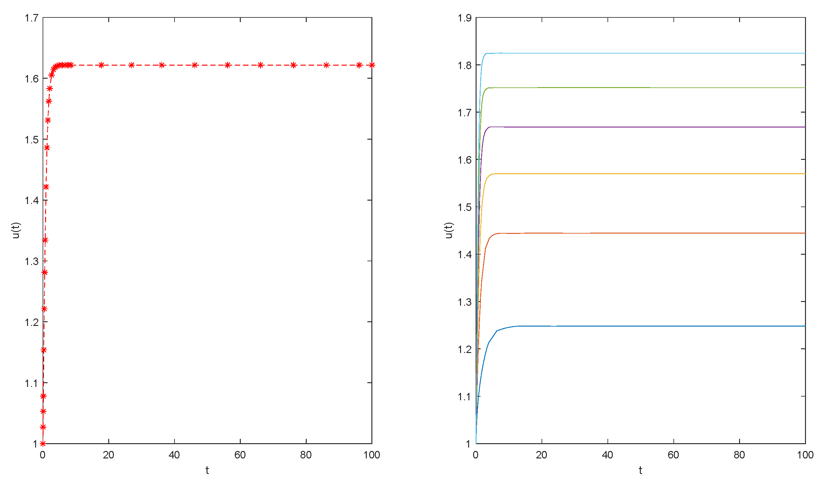
The paper deals with an analysis of the ternary nonlinear dynamical FitzHugh–Rinzel system. Properties of solutions are investigated and, by means of a suitable “energy function”, conditions that ensure the boundedness and existence of absorbing sets in the energy phase space are given. Moreover, according to the parameters characterizing the system, an example has been considered showing that, even with only one choice of parameters, the variable a allows us to obtain several classes of bounded solutions. Moreover, by choosing the value of parameters in accordance with the assumptions of Theorem 1, by means of a first integral of the FHR system (7), some graphs of numerical solutions have been obtained, showing bounded solutions as predicted by theory.

The present results will be quite useful when the analysis is turned to a different physical case. Indeed, the constant a introduced in the FHR model (6) generalizes the FHR system (7), and the results obtained do not directly involve the limits on $a,$ thus suggesting the possibility of generalizing the results.

Moreover, the scientific methodology employed can be applied in multiple scientific fields given the equivalence that such a mathematical model creates between biological problems and electrical transmission phenomena, such as in the superconducting processes of Josephson junctions. In this type of junction, a third-order partial differential equation, similar to the one introduced in [5] and extensively discussed in [13,14,15,16,17], describes the motion of squids in superconductivity. This suggests that the analysis of such models is reflected in a vast number of realistic mathematical models. Finally, it is important to underline that the existence of bounded solutions and absorbing sets paves the way for further research both into stability problems and in the Hopf bifurcations that are so essential for the study of bursting oscillations.

References

- Keener, J.P.; Sneyd, J. Mathematical Physiology; Springer: New York, NY, USA, 1998. [Google Scholar]
- Murray, J.D. Mathematical Biology I; Springer: New York,, NY, USA, 2002. [Google Scholar]
- Izhikevich, E.M. Dynamical Systems in Neuroscience: The Geometry of Excitability and Bursting; The MIT Press: London, UK, 2007. [Google Scholar]
- Izhikovich, E.M. Neural excitability, spiking and bursting. Int. J. Bifurc. Chaos 2000, 10, 1171–1266. [Google Scholar] [CrossRef]
- Nagumo, J.; Arimoto, S.; Yoshizawa, S. An Active Pulse Transmission Line Simulating Nerve Axon. Proc. IRE 1962, 50, 2061–2070. [Google Scholar] [CrossRef]
- Hodgin, A.I.; Huxley, A. Quantitative description of membrane currents and its applications to conduction and excitation in Nerve. J. Physiol. 1952, 112, 500–544. [Google Scholar] [CrossRef]
- De Angelis, M.; Renno, P. Asymptotic effects of boundary perturbations in excitable systems. Discret. Contin. Dyn. Syst. Ser. D 2014, 19, 2039–2045. [Google Scholar] [CrossRef]
- Kudryashov, N.A.; Rybka, K.R.; Sboev, A. Analytical properties of the perturbed FitzHugh-Nagumo model. Appl. Math. Lett. 2018, 76, 142–147. [Google Scholar] [CrossRef]
- De Angelis, M. A priori estimates for excitable models. Meccanica 2013, 48, 2491–2496. [Google Scholar] [CrossRef]
- Torcicollo, I. On the non-linear stability of a continuous duopoly model with constant conjectural variation. Int. J. Non-Linear Mech. 2016, 81, 268–273. [Google Scholar] [CrossRef]
- De Angelis, M. A wave equation perturbed by viscous terms: Fast and slow times diffusion effects in a Neumann problem. Ric. Mat. 2019, 68, 237–252. [Google Scholar] [CrossRef]
- Gambino, G.; Lombardo, M.C.; Giunta, V.; Rubino, G. Cross-diffusion effects on stationary pattern formation in the FitzHugh-Nagumo model. Discret. Contin. Dyn. Syst. -Ser. B 2022. [Google Scholar] [CrossRef]
- De Angelis, M.; Fiore, G. Diffusion effects in a superconductive model. Commun. Pure Appl. Anal. 2014, 13, 217–223. [Google Scholar] [CrossRef]
- Scott, A.C. The Nonlinear Universe Chaos, Emergence, Life; Springer: Berlin/Heidelberg, Germany, 2007. [Google Scholar]
- De Angelis, M.; Renno, P. On Asymptotic Effects of Boundary Perturbations in Exponentially Shaped Josephson Junctions. Acta Appl. Math. 2014, 132, 251–259. [Google Scholar] [CrossRef]
- Scott, A.C. Neuroscience: A Mathematical Primer; Springer: New York, NY, USA, 2002. [Google Scholar]
- De Angelis, M. On the transition from parabolicity to hyperbolicity for a nonlinear equation under Neumann boundary conditions. Meccanica 2018, 53, 3651–3659. [Google Scholar] [CrossRef]
- Lin, V.; Liu, W.B.; Bao, H.; Shen, Q. Bifurcation mechanism of periodic bursting in a simple three-element-based memristive circuit with fast-slow effect. Chaos Solitons Fractals 2020, 131, 109524. [Google Scholar] [CrossRef]
- Juzekaeva, E.; Nasretdinov, A.; Battistoni, S.; Berzina, T.; Iannotta, S.; Khazipov, R.; Erokhin, V.; Mukhtarov, M. Coupling Cortical Neurons through Electronic Memristive Synapse. Adv. Mater. Technol. 2019, 4, 1800350. [Google Scholar] [CrossRef]
- Bertram, R.; Manish, T.; Butte, J.; Kiemel, T.; Sherman, A. Topological and phenomenological classification of bursting oscillations. Bull. Math. Biol. 1995, 57, 413. [Google Scholar] [CrossRef]
- Quarteroni, A.; Manzoni, A.; Vergara, C. The cardiovascular system:mathematical modelling, numerical algorithms and clinical applications. Acta Numer. 2017, 26, 365–590. [Google Scholar] [CrossRef]
- Carillo, S.; Schiebold, C. Construction of Soliton Solutions of the Matrix Modified Korteweg–de Vries Equation. In Advances in Nonlinear Dynamics; NODYCON Conference Proceedings Series; Lacarbonara, W., Balachandran, B., Leamy, M.J., Ma, J., Tenreiro Machado, J.A., Stepan, G., Eds.; Springer: Cham, Switzerland, 2022; pp. 481–495. [Google Scholar]
- De Angelis, M. A Note on Explicit Solutions of FitzHugh-Rinzel System. Nonlinear Dyn. Syst. Theory 2021, 21, 360–366. [Google Scholar] [CrossRef]
- Li, H.; Guoa, Y. New exact solutions to the Fitzhugh Nagumo equation. Appl. Math. Comput. 2006, 180, 524–528. [Google Scholar] [CrossRef]
- Zemlyanukhin, A.I.; Bochkarev, A.V. Analytical Properties and Solutions of the FitzHugh–Rinzel Model. Rus. J. Nonlin. Dyn. 2019, 15, 3–12. [Google Scholar] [CrossRef]
- De Angelis, F.; De Angelis, M. On solutions to a FitzHugh–Rinzel type model. Ric. Mat. 2021, 70, 51–65. [Google Scholar] [CrossRef]
- Smoller, J. Shock Waves and Reaction-Diffusion Equations, 2nd ed.; Springer: New York, NY, USA, 1994. [Google Scholar]
- Capone, F.; Carfora, M.F.; De Luca, R.; Torcicollo, I. Turing patterns in a reaction–diffusion system modeling hunting cooperation. Math. Comput. Simul. 2019, 165, 172–180. [Google Scholar] [CrossRef]
- De Angelis, M. A priori estimates for solutions of FitzHugh–Rinzel system. Meccanica 2022, 57, 1035–1045. [Google Scholar] [CrossRef]
- Rionero, S. Longtime behaviour and bursting frequency, via a simple formula, of FitzHugh–Rinzel neurons. Rend. Lincei. Sci. Fis. e Nat. 2021, 32, 857–867. [Google Scholar] [CrossRef]
- Xie, W.; Xu, J.; Cai, L.; Jin, Y. Dynamics and geometric desingularization of the multiple time scale Fitzhugh Nagumo Rinzel model with fold singularity. Commun. Nonlinear Sci. Numer. Simul. 2018, 63, 322–338. [Google Scholar] [CrossRef]
- Gutman, M.; Aviram, I.; Rabinovitch, A. Abnormal frequency locking and the function of the cardiac pacemaker. Phys. Rev. E 2004, 70, 037202. [Google Scholar] [CrossRef] [PubMed]
- Dikansky, A. Fitzhugh-Nagumo equations in a nonhomogeneous medium. Discret. Contin. Dyn. Syst. 2005, 2005, 216–224. [Google Scholar]
- Faghih, R.T.; Savla, K.; Dahleh, M.A.; Brown, E.N. Broad Range of Neural Dynamics From a Time-Varying FitzHugh–Nagumo Model and its Spiking Threshold Estimation. IEEE Trans. Biomed. Eng. 2012, 59, 816–823. [Google Scholar] [CrossRef]
- Rinzel, J. A Formal Classification of Bursting Mechanisms in Excitable Systems. In Mathematical Topics in Population Biology, Morphogenesis and Neurosciences; Lecture Notes in Biomathematics; Teramoto, E., Yumaguti, M., Eds.; Springer: Berlin/Heidelberg, Germany, 1987; Volume 71, pp. 8–26. [Google Scholar]
- Rocsoreanu, C.; Georgescu, A.; Giurgiteanu, N. The FitzHugh-Nagumo Model: Bifurcation and Dynamics; Springer Science Business Media: Berlin/Heidelberg, Germany, 2012; Volume 10. [Google Scholar]
Figure 1.
On the left: the bounded solution u(t) when , On the right: the bounded functions as .
Publisher’s Note: MDPI stays neutral with regard to jurisdictional claims in published maps and institutional affiliations. |
© 2022 by the author. Licensee MDPI, Basel, Switzerland. This article is an open access article distributed under the terms and conditions of the Creative Commons Attribution (CC BY) license (https://creativecommons.org/licenses/by/4.0/).
Share and Cite
MDPI and ACS Style
De Angelis, M. Transport Phenomena in Excitable Systems: Existence of Bounded Solutions and Absorbing Sets. Mathematics 2022, 10, 2041. https://0-doi-org.brum.beds.ac.uk/10.3390/math10122041
AMA Style
De Angelis M. Transport Phenomena in Excitable Systems: Existence of Bounded Solutions and Absorbing Sets. Mathematics. 2022; 10(12):2041. https://0-doi-org.brum.beds.ac.uk/10.3390/math10122041
Chicago/Turabian StyleDe Angelis, Monica. 2022. "Transport Phenomena in Excitable Systems: Existence of Bounded Solutions and Absorbing Sets" Mathematics 10, no. 12: 2041. https://0-doi-org.brum.beds.ac.uk/10.3390/math10122041
Note that from the first issue of 2016, this journal uses article numbers instead of page numbers. See further details here.