
LSTM-Based Broad Learning System for Remaining Useful Life Prediction


1
School of Management, Hefei University of Technology, Hefei 230009, China
2
School of Software, Tsinghua University, Beijing 100084, China
*
Author to whom correspondence should be addressed.
Mathematics 2022, 10(12), 2066; https://0-doi-org.brum.beds.ac.uk/10.3390/math10122066
Submission received: 11 May 2022
/
Revised: 7 June 2022
/
Accepted: 13 June 2022
/
Published: 15 June 2022
(This article belongs to the Special Issue Artificial Intelligence and Machine Learning Based Methods and Applications)
Abstract
:Prognostics and health management (PHM) are gradually being applied to production management processes as industrial production is gradually undergoing a transformation, turning into intelligent production and leading to increased demands on the reliability of industrial equipment. Remaining useful life (RUL) prediction plays a pivotal role in this process. Accurate prediction results can effectively provide information about the condition of the equipment on which intelligent maintenance can be based, with many methods applied to this task. However, the current problems of inadequate feature extraction and poor correlation between prediction results and data still affect the prediction accuracy. To overcome these obstacles, we constructed a new fusion model that extracts data features based on a broad learning system (BLS) and embeds long short-term memory (LSTM) to process time-series information, named as the B-LSTM. First, the LSTM controls the transmission of information from the data to the gate mechanism, and the retained information generates the mapped features and forms the feature nodes. Then, the random feature nodes are supplemented by an activation function that generates enhancement nodes with greater expressive power, increasing the nonlinear factor in the network, and eventually the feature nodes and enhancement nodes are jointly connected to the output layer. The B-LSTM was experimentally used with the C-MAPSS dataset and the results of comparison with several mainstream methods showed that the new model achieved significant improvements.
1. Introduction
Remaining useful life (RUL) is the length of time that an equipment component or system can operate from the current point in time until the point in time at which it is no longer able to perform a specific function [1]. During the operation of equipment, internal and external factors such as high temperature and corrosive working environment, overload operation and illegal operation will cause the performance and health of its components to deteriorate gradually. If appropriate maintenance measures are not taken before components lose their function, not only will the normal operation of the equipment be affected, but there is a risk of damage to the equipment due to damaged components. By continuously monitoring and analyzing the equipment’s operating data, RUL prediction helps managers make maintenance or replacement decisions before parts are damaged, ensuring the reliability and safety of system operation and reducing economic losses. Therefore, accurate prediction is essential for maintaining normal production. There are three main types of prediction methods: (1) physics-based methods; (2) data-driven methods; and (3) methods that integrate these two approaches [2,3]. In physics-based methods, a mathematical model is usually constructed to describe the failure mechanism based on a particular piece of equipment and combined with the empirical knowledge of that equipment and the defect growth equation [4,5] to predict the RUL of the equipment. A model-based prognostic method was developed to overcome the influence of the number of sensors on the prediction results. The method is not only an innovation in prediction methods, but also demonstrated the superiority of the approach in reducing the sensor set [6]. Model-based approaches have been shown to be robust in limited sensing scenes. In addition, a method was proposed for online evaluation in cases where little is known about the degradation process and extreme cases are considered: the entire degradation process from start of operation to failure is not observed [7]. El Mejdoubi et al. [8] considered aging conditions in predicting the RUL of supercapacitors where the posterior values of capacitance and resistance are predicted by means of particle filters. Gears are important transmission components and accurate RUL prediction is very important to determine the condition of gearing systems. The accuracy of prediction using the digital twin method was significantly improved due to its comprehensive health indicators [9]. However, physics-based methods require corresponding degradation models based on specific objects and usually are not universal. In addition, as the complexity of the equipment increases, it becomes difficult to model the failure of system objects, limiting the development of RUL prediction methods by model construction.
There are two important branches of data-driven methods, namely, statistical data-driven methods and machine-learning(ML)-based methods, that are the current mainstream methods for RUL prediction [10]. Statistical data-driven approaches are used to predict system status based on monitoring data through statistical models without making assumptions or empirical estimates of physical parameters. Park and Padgett [11] provided a new model of accelerated degeneracy, mainly for faults in geometric Brownian motion or gamma processes, with approximation operations using Birnbaum–Saunders and inverse Gaussian distributions. Chehade and Hussein [12] proposed a multioutput convolutional Gaussian process (MCGP) model that captures the cross-correlation between the capacities of available battery cells and is very effective for long-term capacity prediction of lithium-ion (Li-ion) batteries. Van Noortwijk et al. [13] proposed a method that combines two stochastic processes to assess reliability over time. In [14], a degradation model based on the Wiener process and using recursive filters to update the drift coefficients was developed to predict the RUL. The prediction accuracy of physics-based methods depends on the choice of degradation model, but the degradation models are distinctive for different types of equipment. By contrast, statistical data-driven methods are valid in overcoming the problems associated with model selection.
Recently, ML has matured in applications such as data mining, speech recognition, computer vision, fault diagnosis and RUL prediction due to its powerful data processing capabilities. ML-based prediction methods can overcome the problem of unknown degradation models, as the input is not limited by the type of data but can be many different types of data. ML used to predict RUL can be divided into shallow ML and deep learning (DL) methods. The common shallow ML prediction methods are back-propagation (BP), extreme learning machines (ELMs), support vector machines (SVMs) and relevance vector machines (RVMs). BP-based neural networks have good long-term predictive capabilities. Gebraeel et al. [15] established neural-network-based models to train the vibration data of the bearings to obtain the expected failure time of the bearings. Since a single BP neural network faces the problem of the weights falling into local optima and slow convergence during training, some approaches combining other methods with BP algorithms have been proposed. In [16], Wang et al. predicted the distribution of RUL of cooling fans by building a time-series ARIMA model; the combination with a BP neural network model improved the feature extraction ability of the model and improved the prediction accuracy. ELMs have features such as fast learning speed and high generalization ability, and these advantages are used in RUL prediction to feed the extracted features into ELM models for training, thus improving the prediction accuracy [17]. Maior et al. [18] presented a method combining empirical mode decomposition and SVM for degradation data analysis and RUL prediction. Improving the accuracy of prediction under uncertainty is a problem that urgently needs to be solved. Wang et al. [19] extended the RVM to the probability manifold to eliminate the negative impact of the RVM evidence approximation and underestimation of hyperparameters on the prediction. Although some studies corroborate the effectiveness of shallow ML in the field of RUL prediction, traditional shallow ML algorithms rely heavily on the prior knowledge of experts and signal processing techniques, making it difficult to automatically process and analyze large amounts of monitoring data.
By contrast, DL models aim to build deep neural network architectures that combine low-dimensional features of the data to form more abstract high-level attributes with strong feature learning capabilities. In 2006, the greedy layer-wise pretraining method was proposed achieved a theoretical breakthrough in DL [20]. Subsequently, DL has had a wide range of applications in several fields, such as image recognition [21], speech recognition [22], fault diagnosis [23] and RUL prediction [24]. Deutsch et al. [25] combined the feature extraction capabilities of DBNs with the superior predictive capabilities of feedforward neural networks (FNNs) in predicting the RUL of rotating equipment. Based on this approach, to obtain the probability distribution of the remaining lifetime, DBN was effectively combined with particle filtering to further improve the prediction accuracy [26]. Deep neural networks (DNNs) have poor long-term prediction accuracy and need to be combined with other methods for better performance. A convolutional neural network (CNN) is a classical feedforward neural network with excellent characteristics such as parameter sharing and spatial pooling. In [27], a deep convolutional neural network (DCNN) and time window approach were utilized for sample preparation and demonstrated the extraction of more efficient features. To facilitate the fusion of comprehensive information, a RUL prediction method was proposed that learns salient features automatically from multiscale convolutional neural networks (MSCNN) and reveals the nonsmoothness of bearing degradation signals through time–frequency representation (TFR) [28]. In contrast to CNNs, recurrent neural networks (RNNs) are feedforward neural networks containing feedforward connections and internal feedback connections. Their special network structure allows the retention of data information of the implicit layer at the previous moment to be preserved and is often used to process monitoring vector sequences with interdependent properties. Heimes [29] realized the prediction of the RUL based on the RNN structure. However, due to the problems of vanishing and exploding gradients, RNNs processing long-term monitoring sequences produce large prediction bias [30]. To effectively address long-term sequence problems, LSTM was used on top of RNN, which made some improvements and allowed the gate structure to determine the information features passed under optimal conditions [31]. Zhao et al. [32] constructed a hybrid model based on the capsule neural network and long short-term memory network (Cap-LSTM) to extract multivariate time-series sensor data, where the model is feature sensitive and feature information is fully utilized resulting in improved prediction accuracy. A number of variants have been proposed based on typical LSTM networks. The attention mechanism can highlight key parts of time-series information and improve accuracy when predicting. The local features of the original signal sequence were extracted by a one-dimensional convolutional neural network, combined with a LSTM network and attention mechanism to analyze sensor signals and predict RUL, improving the robustness of the model and obtaining higher prediction accuracy [33]. DL is widely used for RUL prediction due to its feature representation being stronger than shallow ML and its ability to handle large amounts of data.
In addition, hybrid approaches based on physics-based and data-driven approaches were developed, such as the method of Sunet et al. [34], where empirical model decomposition, Wiener processes and neural networks were combined to take full advantage of both physical models and data-driven approaches. However, it is not easy to design a structure that reflects the advantages of both methods; thus, the use of hybrid methods to predict RUL is uncommon.
Although current ML algorithms perform well in the field of RUL prediction, and in particular LSTM is effective in handling time-series data, there are still some drawbacks to overcome when applying ML to RUL prediction. First of all, the existing methods suffer from inadequate feature representation in RUL prediction, which affects their accuracy. Secondly, the existing prediction models have to reconstruct the whole model and retrain the parameters when a new data input is available, which is less efficient. To address this problem, a new LSTM-based BLS algorithm is proposed. On the one hand, the BLS has powerful feature representation and prediction capabilities and can accurately represent the relationship between data characteristics and predicted outcomes. Meanwhile, compared with DL, the BLS has a simple structure, a high training speed and the advantage of incremental learning. When the network does not reach the expected performance, only incremental learning is required and only the incremental part needs to be computed without rebuilding the entire network. This significantly improves the efficiency of data processing. In addition, LSTM can effectively process time-series data and avoid problems such as parameter setting and single-time prediction randomness. On the other hand, we hope to broaden the theoretical study of BLS networks by constructing a new fusion network and applying it to practical production scenarios to create economic benefits.
We propose a method for predicting RUL that takes into account both feature extraction and time-series information. It is hoped that sufficient feature extraction can improve the prediction performance, and appropriately broaden the theory and application of the BLS. Specifically, the main contributions and innovations of the work we have conducted are listed below:
- (1)
- A new LSTM-based BLS prediction method is proposed to extract the time-series features of the data based on feature extraction, improving the ability of the prediction results to represent the data features and enhancing the RUL prediction accuracy.
- (2)
- The mechanism of model construction represents another innovation. Instead of directly splicing the two methods, the new method is embedded by modifying the internal structure and avoiding the redundancy of the model.
- (3)
- The adaptation on the basis of a BLS enriches the practical significance of the BLS framework, extends the scope of theoretical research and enables the achievement of better results by integrating the BLS with other methods.
The rest of the paper is structured as follows. The constructed B-LSTM model and the required related basics are introduced and presented in Section 2. Section 3 presents the experimental data required and the experimental design. Section 4 applies the dataset for validation of the model performance and comparison with other methods. A summary of the model and possible future research directions are shown in Section 5.
2. Related Work
2.1. Broad Learning System (BLS)
With the continuous development of deep learning, deep networks are widely used in various research fields, but the disadvantages are also more obvious. In order to achieve higher accuracy, the number of network layers has to be gradually increased; however, this consumes more computational resources and causes overfitting to occur in small sample data processing. A BLS is built based on a single hidden layer neural network and uses lateral scaling to improve accuracy and avoid complex hyperparameters. The unique feature node and enhancement node structure also provides a strong guarantee for adequate feature extraction.
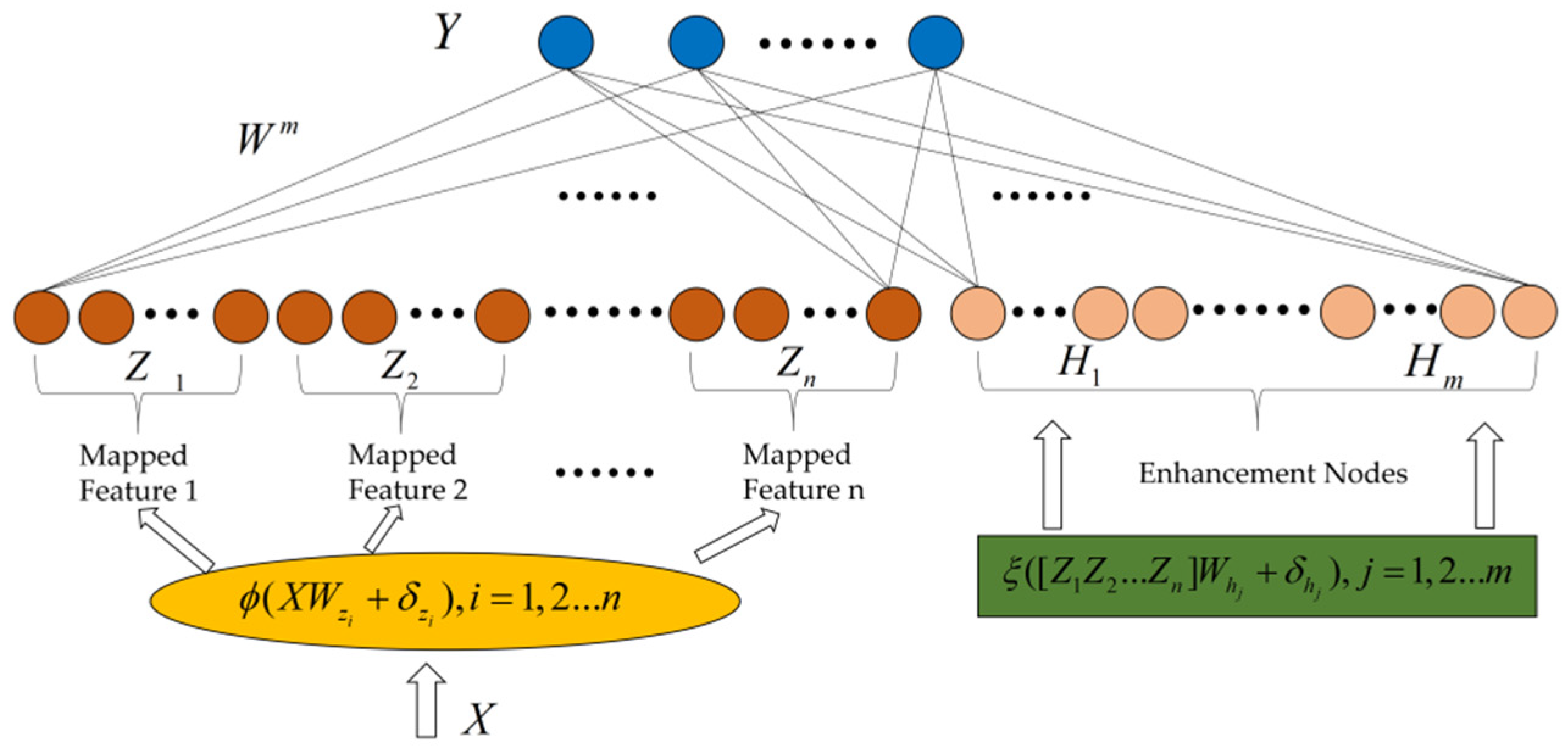
The BLS was established by C. L. Philip Chen on the basis of a random vector functional-link neural network (RVFLLNN) and compensated for its shortcomings in handling large-volume and time-varying data [35]. In addition, the multiple variants proposed in the course of subsequent research showed flexibility, stability and remarkable results in classification and regression of semi-supervised and unsupervised tasks [36]. The structure of the BLS is shown in Figure 1. The network structure is constructed using the following steps. First, the mapping of input data to feature nodes is established, and then the enhancement nodes are formed through a nonlinear activation function. Eventually, the feature nodes and the enhancement nodes are combined as outputs, and the output weight can be directly found through pseudo-inverse ridge regression.
The BLS is constructed as follows:
The given data are subjected to a random weight matrix for feature mapping to obtain a feature matrix with the aim of dimensionality reduction and feature extraction. The th mapped feature is:
Here, the parameters and the bias are randomly initialized. We denote as the collection of groups of feature nodes. Then, they are sent to the enhancement nodes.
Similarly, the th group enhancement nodes are:
By introducing a nonlinear activation function, the feature nodes are mapped nonlinearly to a higher dimensional subspace and the nonlinear element in the network is enhanced. In addition, the outputs of the enhancement layer are denoted as .
Finally, the output of the BLS consists of feature nodes and enhancement nodes together, which can be expressed as follows:
are the weights that connect the feature nodes and the enhancement nodes to the output and , where the pseudo-inverse can be directly calculated by ridge regression.
2.2. Long Short-Term Memory (LSTM)
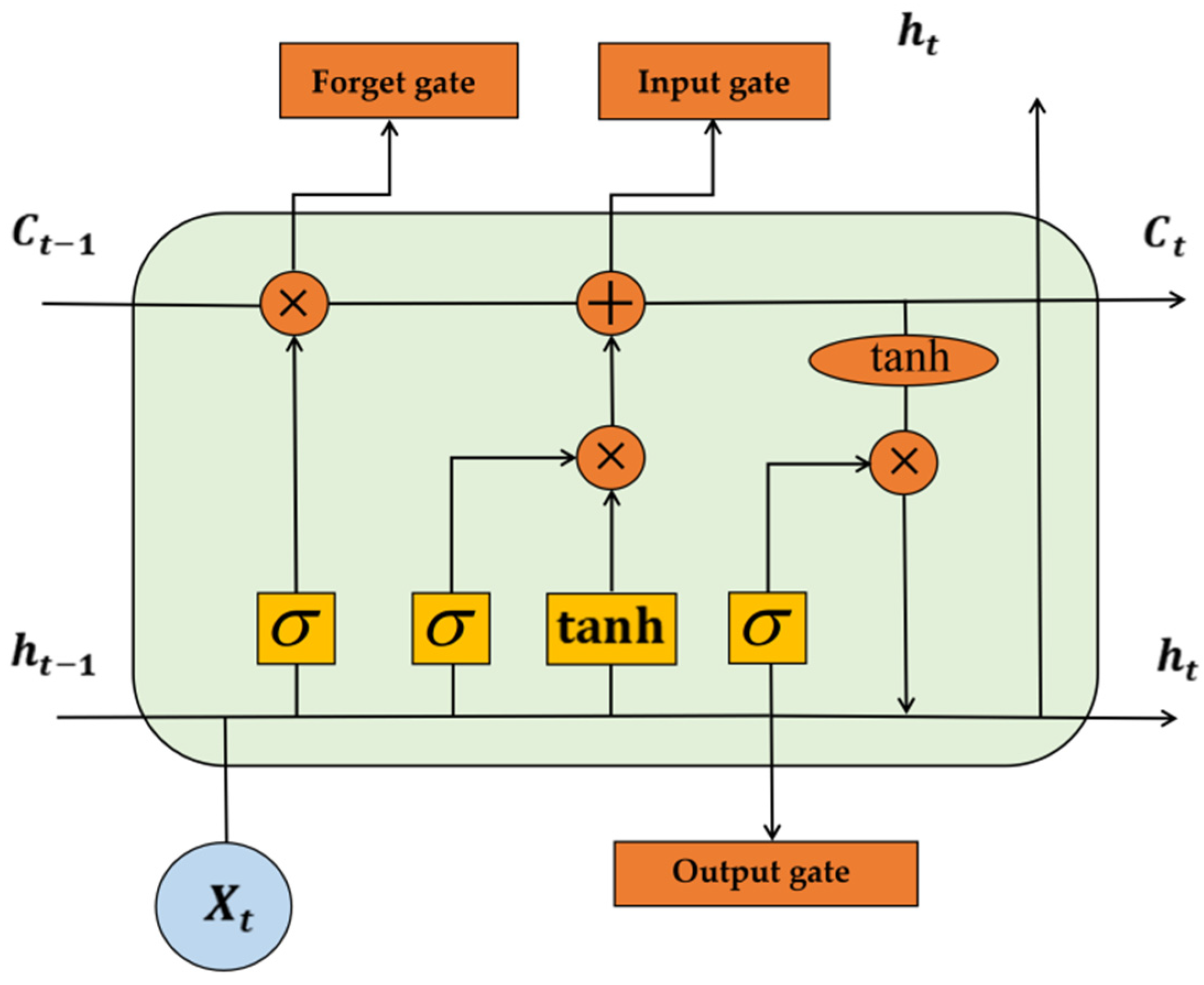
The LSTM network structure is built on top of the RNN. The memory cell structure is illustrated in Figure 2. In dealing with the problem of long-term sequences, a cell state is added, which determines whether past and present information can be added through a gating mechanism, overcoming the “gradient vanishing” and “gradient explosion” problems of the RNN. LSTM has three gates to control the flow of information in the network. The forget gate controls how much of the previous state can be retained. The input gate determines whether to use the current input to update the information of the LSTM. The output gate determines which parts of the current cell state need to be outputted to the next layer for iteration.
where is the data entered into the memory cell for training and is the output in each cell. In addition, , and are the weight matrix and biases, respectively, is the sigmoid activation function used to control the weight of the message passing through and is the dot product.
Specifically, the update process of a cell state can be divided into the following steps: (1) determine what useless information is discarded from the state of the previous time step; (2) extract the valid information that can be added to the state cell at the current time step; (3) calculate the state unit of the current time step; and (4) calculate the output of the current time step.
Variants of LSTM as part of a prediction model that take full advantage of LSTM in processing time-series information are also a common approaches in current research.
2.3. LSTM-Based Broad Learning System (B-LSTM)
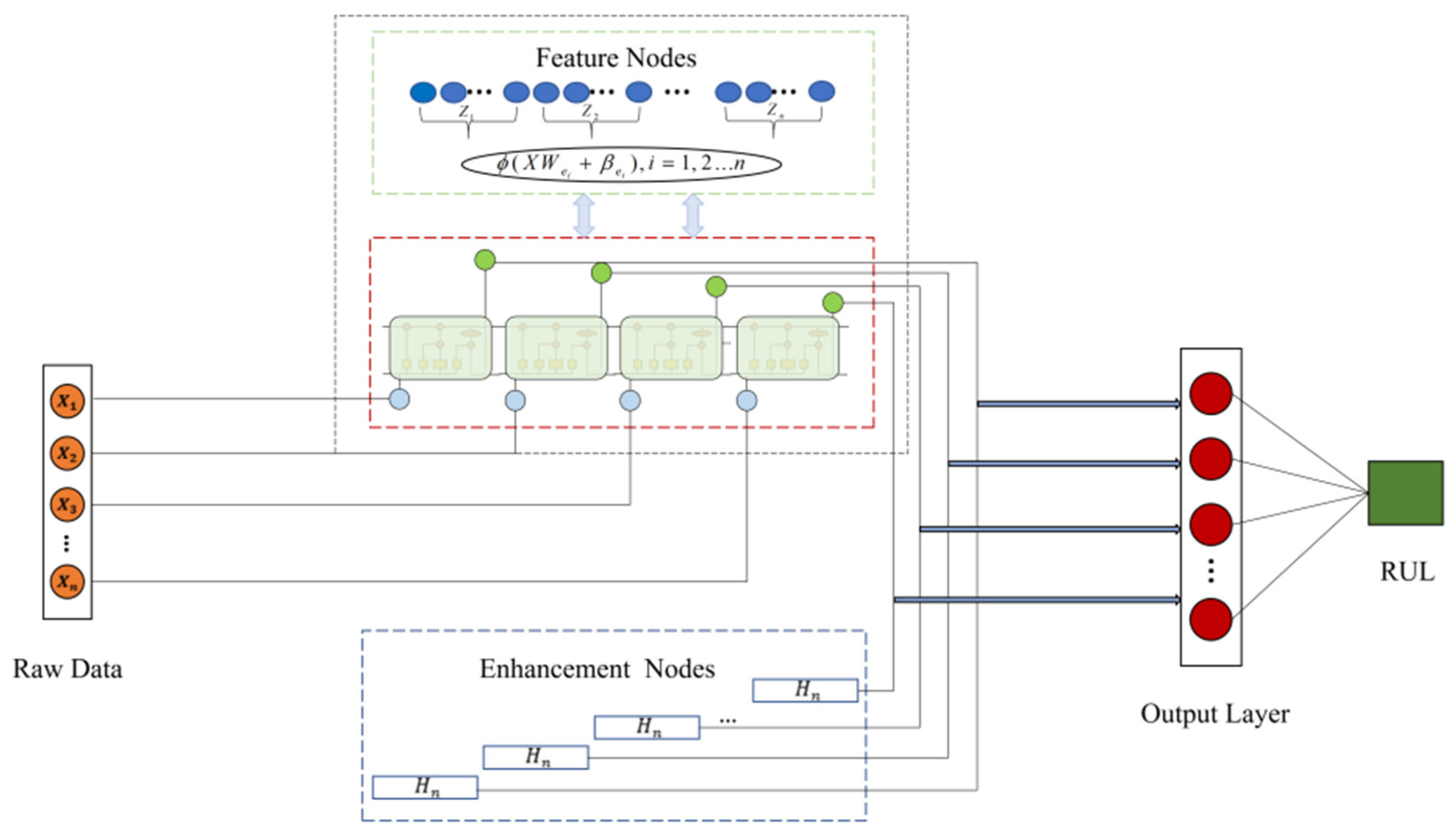
For RUL prediction, more accurate predictions are always obtained by fully learning both the time-series information and feature information of the given data. When performing time-series forecasting, the serial information of the data cannot be learned simply by constructing a framework of mapped features. Therefore, in order to construct a prediction model with comprehensive coverage, a model based on BLS and introducing LSTM is proposed, named B-LSTM. The intuitive idea is to enhance the extraction of time-series information based on the extraction of feature information. The flow is shown in Algorithm 1. In the original BLS framework, each attribute must be independent of the others, and due to this independence, each matrix can learn the features through the variation of different weights. The construction mechanism of the B-LSTM is shown in Figure 3. In this figure, unlike the standard BLS, the raw data are first fed into the LSTM to learn the time-series information. The resulting output is then transformed nonlinearly to generate enhancement nodes that extract deeper features and increase the nonlinear fitting capability of the model. Finally, the state output of the LSTM is connected to the output as a feature layer and an enhancement node. The feature matrix and enhancement matrix of the B-LSTM structure are represented as:
where is the collection of groups of feature nodes obtained by the calculation of the LSTM network. Finally, the connections of all of the mapped features and the enhancement nodes are sent to the output layer. The dynamic equation of B-LSTM is shown below:
| Algorithm 1: B-LSTM Model |
| Input: Training data ; |
| Output: the output weights ; |
| 1: for |
| 2: Calculate ; |
| 3: Calculate |
| 4: end for |
| 5: Set |
| 6: for |
| 7: Random |
| 8: Calculate |
| 9: end for |
| 10: Set |
| 11: Set and calculate Equation (11); |
| 12: Calculate |
3. Experimental Procedure and Analysis
3.1. C-MAPSS Dataset
The C-MAPSS dataset contains aircraft turbofan engine degradation simulation data, including simulated sensor data generated by different turbofan engines over time; this dataset was selected for training and evaluation of the effectiveness of the proposed model. Table 1 shows that the dataset consists of four sub-datasets, FD0001, FD0002, FD0003 and FD0004, where both the FD001 and FD003 datasets contain 1 operational condition and contain 1 and 2 fault types, respectively, whereas FD002 and FD004 both contain 6 operational conditions and contain 1 and 2 fault types, respectively. These sub-datasets consist of engine numbers, serial numbers, configuration items and sensor data obtained from 21 sensors, simulating the progressive degradation of the engine from a healthy state to failure for different initial conditions.
Each of the four sub-datasets contains a training set and a test set in which the actual RUL values of the test engine are also included. The training set includes all data from the start of the turbofan engine’s operation until its degradation and failure. In the test set, however, the data start from a healthy state and are subsequently arbitrarily truncated; the operating time periods up to the point of system failure were calculated from these data.
3.2. Performance Measures
To quantitatively assess the performance of the model, we compared the prediction results of the new model and the predictions of this model were compared with those of other network structures. Two objective evaluation metrics, namely, RMSE and Score, are introduced in this paper, where ; when the prediction error d is 0, RMSE and Score are both the minimum values of 0. As the absolute value of increases, the two evaluation indices are increased. The difference is that when , Score gives different penalty weights for model prediction lag and prediction advance. If the predicted value is smaller than the true value, it means that the prediction is ahead and the penalty coefficient is smaller, and conversely, lagging brings more serious consequences and the penalty coefficient is larger. Predicting the RUL value earlier allows for earlier maintenance planning and avoidance of potential losses.
3.3. Experimental Setup
Our experimental equipment was a personal computer with an Intel Core i5 CPU, 16GB RAM and NVIDIA GTX 1080ti GPU. The operating system was Windows 10 Professional and the programming platform was MATLAB R2019b.
First, data filtering was performed on the dataset, and in each dataset, a single sampled data sample consisted of 26 variables, of which the first 2 variables represented the engine sequence number and the cycle sequence number, the last 3 variables represented the operation setting items and the remaining 21 variables represented the detection values obtained by the 21 sensors. The third position of the operation setting term and the sensor values with sequence numbers 1, 5, 6, 10, 16, 18 and 19 were unchanged and had no effect on the prediction results, so they were filtered out. Then, since the sensors were of different types and the selected data were of different magnitudes, we made the range of values uniform across the data by data normalization. Finally, we divided the data into training and validation sets proportionally, set the training parameters and inputted the processed training and validation sets into the model for model training.
4. Results and Discussion
4.1. RUL Prediction
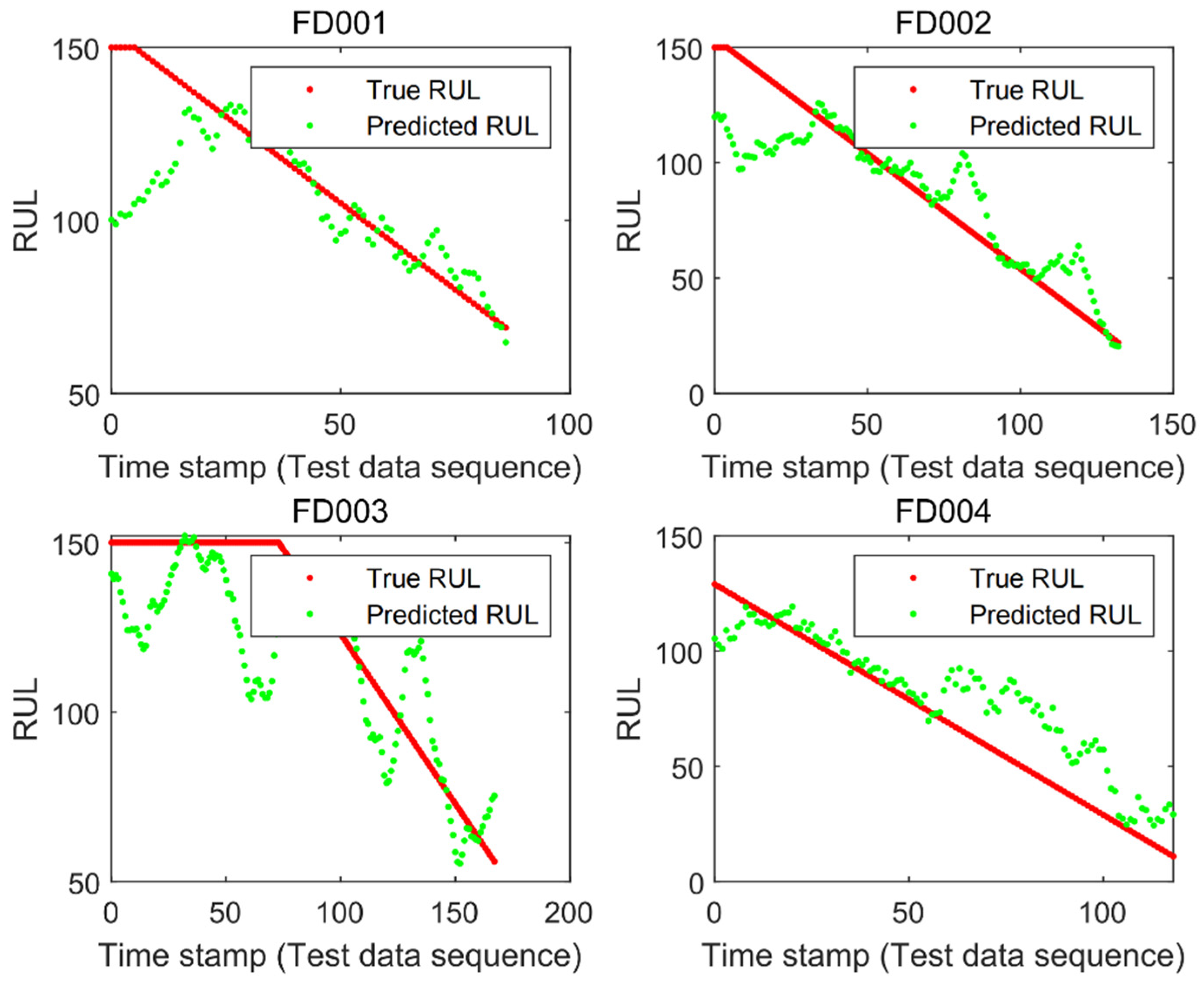
To verify the performance of the B-LSTM model, we inputted the datasets into the model and roughly determined whether the model can effectively predict based on the fit between the true and predicted values of the RUL. The prediction results are shown in Figure 4. The red solid line indicates the true RUL value, whereas the green scatter plot indicates the predicted value. As can be seen from the figure, the B-LSTM was able to depict the trend of RUL variation for each test set. This shows that the improved structure of extracting time-series information and feature information can be more effective in making predictions. In addition, in the FD001 and FD003 datasets, the B-LSTM model made better predictions compared to the other two datasets because in these two sub-datasets the failure modes and operating conditions were relatively simple. Although the operating conditions and failure modes in the FD002 and FD004 test sets were more complex, they basically described the changing trend of the equipment RUL.
We can see that the true value of RUL in the FD003 sub-dataset in the prediction result plot continued to be constant at the beginning; this is because after our practical verification, due to the smoother operating conditions, the RUL in FD003 remained basically stable at the beginning of the operation and can be considered as constant, and only at a later stage did a linear decline occur as the RUL of the device did not change uniformly with time. In order to make better predictions of RUL, we processed the labels of FD003 training data. The RUL was set to a fixed value when the operating cycle of the device was less than 60, and decreased gradually with the growth of the operating cycle when the operating cycle was greater than 60, as the device gradually declined.
4.2. Performance Evaluation
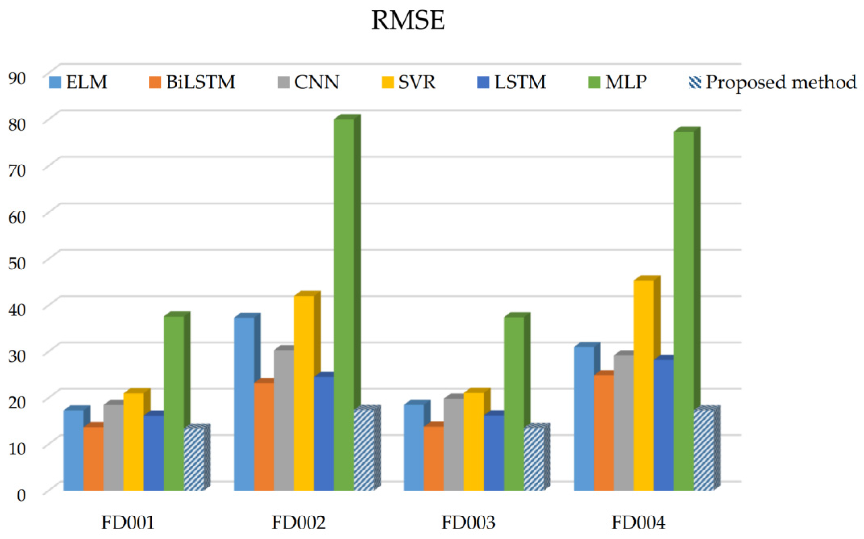
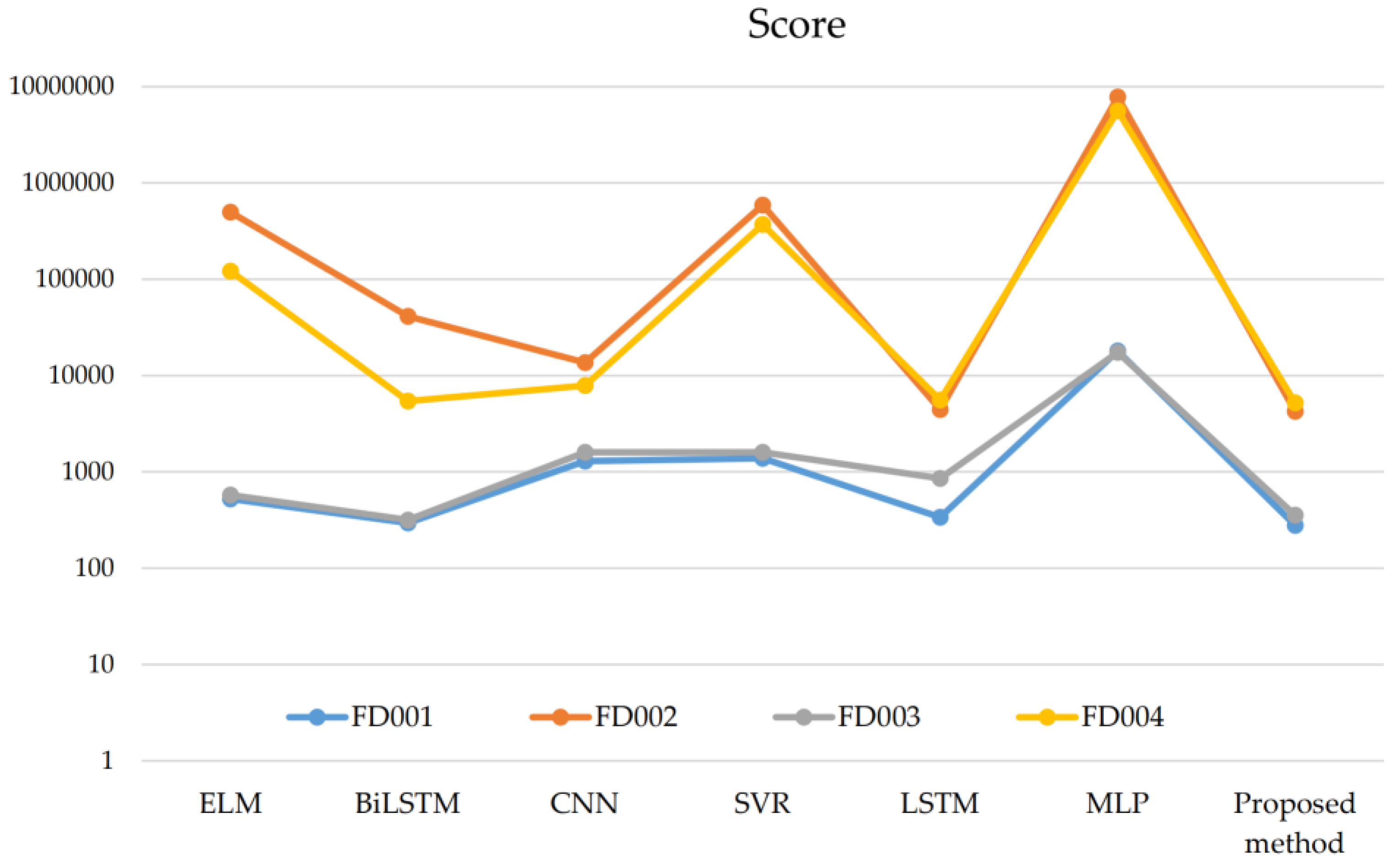
To verify the performance of the model, we compared the proposed method with other existing RUL prediction methods, including MLP [37], SVR [37], CNN [37], LSTM [38], ELM [39], and BiLSTM [40]. The comparison results are shown in Table 2. From Figure 5, we can see that the RMSE of the proposed method was smaller than the other methods in all four sub-datasets, especially in FD001 and FD003, where it achieved good results. Similarly, in Figure 6 it is clear that the Score of the new method improved as compared to the other methods. The comparison results show that the method we constructed can fully extract the features of the data and, thus, obtain more accurate prediction results. In addition, the FD001 and FD003 datasets performed better for each prediction method compared to the other two datasets because the turbine engines in the FD001 and FD003 datasets have fewer operating conditions and can maintain smooth operating conditions during the operating period.
5. Conclusions
There are a variety of methods for predicting RUL in the existing research, but these methods can have some problems in actual prediction, such as ignoring time-series features, features not being sufficiently extracted, etc. We proposed a new method for predicting RUL and demonstrated that the method improves prediction performance. Specifically, a new BLS network integrated with LSTM, named B-LSTM, is essential for enriching the theoretical knowledge of RUL prediction.
Theoretically, this network retains the time-series information in the input data while performing sufficient feature extraction so that the output of the model remains strongly correlated with the input data and the interpretability and accuracy of the model is enhanced. In addition, when the model performance was validated using the C-MAPSS dataset, the results obtained were significantly better than other models. Therefore, the B-LSTM performed well in both theoretical construction and data validation. Although this study achieved ideal conclusions, the experimental results of one dataset may be serendipitous; therefore, in the following research, we will use more different datasets to verify the scientificity and generalizability of the proposed model. In addition, this research did not pay too much attention to the training time of the model. In later work, we will focus on further optimizing the model structure to shorten the training time so that the model can be processed quickly and, at the same time, achieve a satisfactory accuracy.
Author Contributions
Conceptualization, X.W.; writing, manuscript preparation, T.H.; review and editing, K.Z.; supervision and project management, X.Z. All authors have read and agreed to the published version of the manuscript.
Funding
This research received no external funding.
Institutional Review Board Statement
Not applicable.
Informed Consent Statement
Not applicable.
Data Availability Statement
The data of this paper came from the NASA Prognostics Center of Excellence, and the data acquisition website was: https://ti.arc.nasa.gov/tech/dash/groups/pcoe/prognostic-data-repository/#turbofan, accessed on 10 February 2022.
Conflicts of Interest
The authors declare no conflict of interest.
References
- Liu, G. A Study on Remaining Useful Life Prediction for Prognostic Applications. Master’s Thesis, University of New Orleans, New Orleans, LA, USA, 2011. [Google Scholar]
- Zio, E.; Di Maio, F. A data-driven fuzzy approach for predicting the remaining useful life in dynamic failure scenarios of a nuclear system. Reliab. Eng. Syst. Saf. 2010, 95, 49–57. [Google Scholar] [CrossRef] [Green Version]
- Heng, A.; Zhang, S.; Tan, A.; Mathew, J. Rotating machinery prognostics: State of the art, challenges and opportunities. Mech. Syst. Signal Process. 2009, 23, 724–739. [Google Scholar] [CrossRef]
- Li, C.J.; Lee, H. Gear fatigue crack prognosis using embedded model, gear dynamic model and fracture mechanics. Mech. Syst. Signal Process. 2005, 19, 836–846. [Google Scholar] [CrossRef]
- Fan, J.; Yung, K.C.; Pecht, M.; Pecht, M. Physics-of-Failure-Based Prognostics and Health Management for High-Power White Light-Emitting Diode Lighting. IEEE Trans. Device Mater. Reliab. 2011, 11, 407–416. [Google Scholar] [CrossRef]
- Daigle, M.; Goebel, K. Model-based prognostics under limited sensing. In Proceedings of the IEEE Aerospace Conference, Big Sky, MT, USA, 6–13 March 2010; pp. 1–12. [Google Scholar]
- Hu, Y.; Baraldi, P.; Di Maio, F.; Zio, E. Online Performance Assessment Method for a Model-Based Prognostic Approach. IEEE Trans. Reliab. 2015, 65, 1–18. [Google Scholar]
- El Mejdoubi, A.; Chaoui, H.; Sabor, J.; Gualous, H. Remaining useful life prognosis of supercapacitors under temperature and voltage aging conditions. IEEE Trans. Ind. Electron. 2017, 65, 4357–4367. [Google Scholar] [CrossRef]
- He, B.; Liu, L.; Zhang, D. Digital twin-driven remaining useful life prediction for gear performance degradation: A review. J. Comput. Inf. Sci. Eng. 2021, 21, 030801. [Google Scholar] [CrossRef]
- Pei, H.; Hu, C.; Si, X.; Zhang, J.; Pang, Z.; Zhang, P. Review of Machine Learning Based Remaining Useful Life Prediction Methods for Equipment. J. Mech. Eng. 2019, 55, 1–13. [Google Scholar] [CrossRef] [Green Version]
- Park, C.; Padgett, W.J. Accelerated degradation models for failure based on geometric Brownian motion and gamma processes. Lifetime Data Anal. 2005, 11, 511–527. [Google Scholar] [CrossRef]
- Chehade, A.A.; Hussein, A.A. A multi-output convolved Gaussian process model for capacity estimation of electric vehicle li-ion battery cells. In Proceedings of the IEEE Transportation Electrification Conference and Expo (ITEC), Detroit, MI, USA, 19–21 June 2019; pp. 1–4. [Google Scholar]
- Van Noortwijk, J.M.; van der Weide, J.A.; Kallen, M.J.; Pandey, M.D. Gamma processes and peaks-over-threshold distributions for time-dependent reliability. Reliab. Eng. Syst. Saf. 2007, 92, 1651–1658. [Google Scholar] [CrossRef]
- Si, X.S.; Wang, W.; Hu, C.H.; Chen, M.Y.; Zhou, D.H. A Wiener-process-based degradation model with a recursive filter algorithm for remaining useful life estimation. Mech. Syst. Signal Process. 2013, 35, 219–237. [Google Scholar] [CrossRef]
- Gebraeel, N.; Lawley, M.; Liu, R.; Parmeshwaran, V. Residual life predictions from vibration-based degradation signals: A neural network approach. IEEE Trans. Ind. Electron. 2004, 51, 694–700. [Google Scholar] [CrossRef]
- Lixin, W.; Zhenhuan, W.; Yudong, F.; Guoan, Y. Remaining life predictions of fan based on time series analysis and BP neural networks. In Proceedings of the IEEE Information Technology, Networking, Electronic and Automation Control Conference, Chongqing, China, 20–22 May 2016; pp. 607–611. [Google Scholar]
- Liu, Y.; He, B.; Liu, F.; Lu, S.; Zhao, Y.; Zhao, J. Remaining useful life prediction of rolling bearings using PSR, JADE, and extreme learning machine. Math. Probl. Eng. 2016, 2016, 1–13. [Google Scholar] [CrossRef] [Green Version]
- Maior, C.B.S.; das Chagas Moura, M.; Lins, I.D.; Droguett, E.L.; Diniz, H.H.L. Remaining Useful Life Estimation by Empirical Mode Decomposition and Support Vector Machine. IEEE Lat. Am. Trans. 2016, 14, 4603–4610. [Google Scholar] [CrossRef]
- Wang, X.; Jiang, B.; Ding, S.X.; Lu, N.; Li, Y. Extended Relevance Vector Machine-Based Remaining Useful Life Prediction for DC-Link Capacitor in High-Speed Train; IEEE: Piscataway Township, NJ, USA, 1963; pp. 1–10. [Google Scholar]
- Hinton, G.E.; Osindero, S.; Teh, Y.W. A Fast Learning Algorithm for Deep Belief Nets. Neural Comput. 2006, 18, 1527–1554. [Google Scholar] [CrossRef] [PubMed]
- Shah, S.A.A.; Bennamoun, M.; Boussaid, F. Iterative deep learning for image set based face and object recognition. Neurocomputing 2016, 174, 866–874. [Google Scholar] [CrossRef]
- Deng, L. Deep learning: From speech recognition to language and multimodal processing. APSIPA Trans. Signal Inf. Process. 2016, 5, e1. [Google Scholar] [CrossRef]
- He, M.; He, D. Deep learning based approach for bearing fault diagnosis. IEEE Trans. Ind. Appl. 2017, 53, 3057–3065. [Google Scholar] [CrossRef]
- Ren, L.; Cui, J.; Sun, Y.; Cheng, X. Multi-bearing remaining useful life collaborative prediction: A deep learning approach. J. Manuf. Syst. 2017, 43, 248–256. [Google Scholar] [CrossRef]
- Deutsch, J.; He, D. Using deep learning based approaches for bearing remaining useful life prediction. In Proceedings of the Annual Conference of the PHM Society 2016, Chengdu, China, 19–21 October 2016. [Google Scholar]
- Deutsch, J.; He, M.; He, D. Remaining useful life prediction of hybrid ceramic bearings using an integrated deep learning and particle filter approach. Appl. Sci. 2017, 7, 649. [Google Scholar] [CrossRef] [Green Version]
- Li, X.; Ding, Q.; Sun, J.Q. Remaining useful life estimation in prognostics using deep convolution neural networks. Reliab. Eng. Syst. Saf. 2018, 172, 1–11. [Google Scholar] [CrossRef] [Green Version]
- Zhu, J.; Chen, N.; Peng, W. Estimation of bearing remaining useful life based on multiscale convolutional neural network. IEEE Trans. Ind. Electron. 2018, 66, 3208–3216. [Google Scholar] [CrossRef]
- Heimes, F.O. Recurrent neural networks for remaining useful life estimation. In Proceedings of the International Conference on Prognostics and Health Management, Denver, CO, USA, 6–9 October 2008; pp. 1–6. [Google Scholar]
- Pascanu, R.; Mikolov, T.; Bengio, Y. On the difficulty of training recurrent neural networks, In International conference on machine learning. Proc. Mach. Learn. Res. 2013, 23, 1310–1318. [Google Scholar]
- Wu, Y.; Yuan, M.; Dong, S.; Lin, L.; Liu, Y. Remaining useful life estimation of engineered systems using vanilla LSTM neural networks. Neurocomputing 2018, 275, 167–179. [Google Scholar] [CrossRef]
- Zhao, C.; Huang, X.; Li, Y.; Li, S. A Novel Cap-LSTM Model for Remaining Useful Life Prediction. IEEE Sens. J. 2021, 21, 23498–23509. [Google Scholar] [CrossRef]
- Zhang, H.; Zhang, Q.; Shao, S.; Niu, T.; Yang, X. Attention-based LSTM network for rotatory machine remaining useful life prediction. IEEE Access 2020, 8, 132188–132199. [Google Scholar] [CrossRef]
- Sun, H.; Cao, D.; Zhao, Z.; Kang, X. A hybrid approach to cutting tool remaining useful life prediction based on the Wiener process. IEEE Trans. Reliab. 2018, 67, 1294–1303. [Google Scholar] [CrossRef]
- Chen, C.P.; Liu, Z. Broad Learning System: An Effective and Efficient Incremental Learning System without the Need for Deep Architecture. IEEE Trans. Neural Netw. Learn. Syst. 2018, 29, 10–24. [Google Scholar] [CrossRef]
- Gong, X.; Zhang, T.; Chen, C.P.; Liu, Z. Research Review for Broad Learning System: Algorithms, Theory, and Applications; IEEE: Piscataway Township, NJ, USA, 1963; pp. 1–29. [Google Scholar]
- Sateesh Babu, G.; Zhao, P.; Li, X.L. Deep convolutional neural network based regression approach for estimation of remaining useful life. In International Conference on Database Systems for Advanced Applications; Springer: Berlin/Heidelberg, Germany, 2016; pp. 214–228. [Google Scholar]
- Zheng, S.; Ristovski, K.; Farahat, A.; Gupta, C. Long short-term memory network for remaining useful life estimation. In Proceedings of the 2017 IEEE International Conference on Prognostics and Health Management (ICPHM), Dallas, TX, USA, 19–21 June 2017; pp. 88–95. [Google Scholar]
- Zhang, C.; Lim, P.; Qin, A.K.; Tan, K.C. Multiobjective deep belief networks ensemble for remaining useful life estimation in prognostics. IEEE Trans. Neural Netw. Learn. Syst. 2016, 28, 2306–2318. [Google Scholar] [CrossRef]
- Wang, J.; Wen, G.; Yang, S.; Liu, Y. Remaining useful life estimation in prognostics using deep bidirectional lstm neural network. In Proceedings of the 2018 Prognostics and System Health Management Conference (PHM-Chongqing), Chongqing, China, 26–28 October 2018. [Google Scholar]
Figure 1.
Structure of the BLS network. The Yellow ellipse on the left is the calculation formula for converting input data into feature nodes, the earthy yellow circle on the left is the generated feature nodes, the green rectangle on the right is the calculation formula for converting the left feature nodes into enhancement nodes, the light yellow circle on the right is the generated enhancement nodes, and the blue circle on the top is the output.

Figure 2.
Long short-term cell structure. The blue circle at the bottom is the input data of a cell of the LSTM. The orange rectangular part is the forget gate, input gate and output gate. The yellow part is the calculation formula for generating forget gate, input gate and output gate. The orange circular part is the operator for generating forget gate, input gate and output gate.

Figure 3.
Structure of the B-LSTM network. Multiple orange circles in the left rectangle are the input data. The upper part in the middle indicates that the feature nodes of the new model are replaced by LSTM, the yellow circle in the LSTM part is the input data, the green circle is the feature nodes output by the new model, the lower part in the middle is the enhancement nodes generated by the feature nodes generated by LSTM, the feature nodes and enhancement nodes are connected to the output together, and the red circle on the right is the output of the model.

Figure 4.
B-LSTM-based prediction results.

Figure 5.
The results of RMSE comparison among different methods.

Figure 6.
The results of Score comparison among different methods.


Table 1.
Parameters of the dataset.
| Sub-Dataset | C-MAPSS | |||
|---|---|---|---|---|
| FD001 | FD002 | FD003 | FD004 | |
| Training trajectories | 100 | 260 | 100 | 249 |
| Testing trajectories | 100 | 259 | 100 | 248 |
| Operating conditions | 1 | 6 | 1 | 6 |
| Fault modes | 1 | 1 | 2 | 2 |
Table 2.
Model performance comparison on the C-MAPSS dataset.
| Method | RMSE/Score | |||
|---|---|---|---|---|
| FD001 | FD002 | FD003 | FD004 | |
| MLP | 37.56/18,000 | 80.03/7,800,000 | 37.39/17,400 | 77.37/5,620,000 |
| SVR | 20.96/1380 | 42.0/590,000 | 21.05/1600 | 45.35/371,000 |
| CNN | 18.45/1290 | 30.29/13,600 | 19.82/1600 | 29.16/7890 |
| LSTM | 16.14/338 | 24.49/4450 | 16.18/852 | 28.17/5550 |
| ELM | 17.27/523 | 37.28/498,000 | 18.47/574 | 30.96/121,000 |
| BiLSTM | 13.65/295 | 23.18/41,300 | 13.74/317 | 24.86/5430 |
| Proposed method | 12.45/279 | 15.36/4250 | 13.37/356 | 16.24/5220 |
Publisher’s Note: MDPI stays neutral with regard to jurisdictional claims in published maps and institutional affiliations. |
© 2022 by the authors. Licensee MDPI, Basel, Switzerland. This article is an open access article distributed under the terms and conditions of the Creative Commons Attribution (CC BY) license (https://creativecommons.org/licenses/by/4.0/).
Share and Cite
MDPI and ACS Style
Wang, X.; Huang, T.; Zhu, K.; Zhao, X. LSTM-Based Broad Learning System for Remaining Useful Life Prediction. Mathematics 2022, 10, 2066. https://0-doi-org.brum.beds.ac.uk/10.3390/math10122066
AMA Style
Wang X, Huang T, Zhu K, Zhao X. LSTM-Based Broad Learning System for Remaining Useful Life Prediction. Mathematics. 2022; 10(12):2066. https://0-doi-org.brum.beds.ac.uk/10.3390/math10122066
Chicago/Turabian StyleWang, Xiaojia, Ting Huang, Keyu Zhu, and Xibin Zhao. 2022. "LSTM-Based Broad Learning System for Remaining Useful Life Prediction" Mathematics 10, no. 12: 2066. https://0-doi-org.brum.beds.ac.uk/10.3390/math10122066
Note that from the first issue of 2016, this journal uses article numbers instead of page numbers. See further details here.