
Modified Erlang Loss System for Cognitive Wireless Networks


1
Institute of Applied Mathematical Research, Karelian Research Centre RAS, 185910 Petrozavodsk, Russia
2
Institute of Mathematics and Information Technologies, Petrozavodsk State University, 185910 Petrozavodsk, Russia
3
Moscow Center for Fundamental and Applied Mathematics, Moscow State University, 119991 Moscow, Russia
4
Graduate School of Science and Technology, University of Tsukuba, 1-1-1 Tennodai, Tsukuba 305-8573, Ibaraki, Japan
5
Faculty of Engineering, Information and Systems, University of Tsukuba, 1-1-1 Tennodai, Tsukuba 305-8573, Ibaraki, Japan
*
Authors to whom correspondence should be addressed.
Mathematics 2022, 10(12), 2101; https://0-doi-org.brum.beds.ac.uk/10.3390/math10122101
Submission received: 18 May 2022
/
Revised: 14 June 2022
/
Accepted: 15 June 2022
/
Published: 16 June 2022
(This article belongs to the Special Issue Mathematical Modeling, Optimization and Machine Learning)
Abstract
:This paper considers a modified Erlang loss system for cognitive wireless networks and related applications. A primary user has pre-emptive priority over secondary users, and the primary customer is lost if upon arrival all the channels are used by other primary users. Secondary users cognitively use idle channels, and they can stay (either in an infinite buffer or in an orbit) in cases where idle channels are not available upon arrival or they are interrupted by primary users. While the infinite buffer model represents the case with zero sensing time, the infinite orbit model represents the case with positive sensing time. We obtain an explicit stability condition for the cases where arrival processes of primary users and secondary users follow Poisson processes, and their service times follow two distinct arbitrary distributions. The stability condition is insensitive to the service time distributions and implies the maximal throughout of secondary users. Moreover, we extend the stability analysis to the system with outgoing calls. For a special case of exponential service time distributions, we analyze the buffered system in depth to show the effect of parameters on the delay performance and the mean number of interruptions of secondary users. Our simulations for distributions rather than exponential reveal that the mean number of terminations for secondary users is less sensitive to the service time distribution of primary users.
Keywords:
cognitive wireless network; regenerative analysis; stability condition; priority queue; Erlang loss system; classical retrials; outgoing callsMSC:
90B22; 60K25; 68M201. Introduction
In recent years, Internet traffic has increased explosively due to the increased use of smartphones, tablet computers, etc. This causes a shortage problem of the wireless spectrum. Cognitive wireless is considered a promising solution to this problem [1,2,3,4,5]. For the recent development of cognitive radio networks, we refer to the survey paper by Ostovar et al. [6]. In wireless networks, secondary users (unlicensed users) are allowed to cognitively use the bandwidths that are originally allocated to primary users (licensed users). Secondary users should use the bandwidths in such a way that does not interfere with the primary users. In particular, secondary users can use the bandwidths only if primary users are not present. To this end, secondary users must be aware of the presence of primary users so as to evacuate upon the arrival of primary users. From this point of view, primary users have absolute priority over secondary users, meaning that the transmission of a secondary user might be interrupted by a primary user. In the first system, we assume that interrupted secondary users evacuate to the head of the buffer and resume their transmission as soon as a channel is available. Then, we extend the stability analysis to a partial retrial system when the secondary users are evacuated to a virtual orbit and then attempt to occupy the channel again. Moreover, the analysis is then extended to the system with outgoing calls, which is initiated during the period that a server is idle.
Motivated by the above situation, we propose analyzing a multiserver (multichannel) queueing system with an infinite buffer for secondary users while primary users have absolute priority over secondary users and are lost if all channels are already occupied by other primary users. Under this assumption (and under Poisson inputs), from the viewpoint of primary users, the system of servers behaves as an Erlang loss system, while from that of secondary users, the system is either an infinite buffer model or a retrial model where secondary users are served when some servers are not occupied by primary users. In our model, the service times of primary and secondary customers follow two distinct arbitrary distributions.
A closely related model is the paper by Mitrani and Avi-Itzhak [7]. In this paper, the author considers an M/M/N system where each server is subject to random breakdowns and repairs. The author analyzes the joint distribution of the queue length and the state of the servers using a generating function approach. The model in [7] can be considered as a model with N primary customers. In our model, primary customers arrive according to a Poisson process, implying that there is an infinite number of primary customers. Akutsu and Phung-Duc [8] examine a closely related Markovian model in which secondary customers first sense the channels before occupying them. The stability condition is conjectured and verified by simulation in [8] and further proved using a Lyapunov function approach [9]. Salameh et al. [10,11] consider models with a limited number of sensing secondary users. Other queueing models of cognitive radio networks could be found in [10,12,13,14,15,16,17]. In [10,13,16,18], the service time distributions of primary and secondary customers are either restricted to Markovian distributions (exponential or phase-type distributions) and/or the assumption that the number of active secondary users are finite. In [14,15,17,19,20,21,22,23], models with a single channel are investigated.
In this paper, we first relax these Markovian assumptions mentioned above by considering arbitrary distributions for the service time of primary users and secondary users. Under these assumptions, we are able to obtain an explicit stability condition. To the best of our knowledge, this is the first analytical result for cognitive radio network models with multiple channels. Moreover, we extend the analysis to a model with the retrial secondary customers and with outgoing calls. Next, assuming exponential service time distributions, we study the model in depth using the matrix analytic method [24].
The priority queues are prevalent among models for service differentiation in communication networks and service systems, and by this reason, applications of our model are not restricted to cognitive wireless networks [25].
The rest of this paper is organized as follows. In Section 2, we describe our model in detail with a focus on the regenerative setting. In Section 3, we present the stability analysis of the basic model and, as a by-product of our analysis, obtain the well-known stability condition of a buffered multiserver multiclass system (see Theorem 2 and Remark 4). In Section 4, we prove the stability condition for the system with retrial secondary customers, while in Section 5, we study a generalization of the latter system to capture the outgoing calls as well. Section 6 presents a detailed analysis for a special case with exponential distributions for which we are able to obtain performance measures. We also present numerical and simulation experiments to show insights into the performance of our system and the sensitivity of service time distribution, while Section 7 concludes our paper.
2. Description of the System
In this section, we consider the following basic modification of the Erlang system with two classes of customers with c identical servers, Poisson inputs with rates , and general independent and identically distributed (iid) service times for class-i customers, . Class-1 customers have pre-emptive priority and are lost if upon arrival all servers are busy with class-1 customers, while class-2 (non-priority) customers stay in the system regardless of the state of the system and wait in the queue, if necessary, according to a non-idling FCFS (first-come-first-served) service discipline. Class-1 and class-2 customers correspond to primary and secondary customers, respectively, while a server is a channel in cognitive radio networks. Denote service rates , where is the (generic) service time of class-i customers . We also denote by the arrival instants of the superposed (Poisson) input with rate , and iid exponential interarrival times with generic interarrival time . By pre-emptive-resume priority, a class-1 customer occupies a server busy by a class-2 customer, provided there are no idle servers upon his arrival.
We deduce the stability conditions of this system based on the regenerative approach. More precisely, we show that the basic processes describing the dynamics of the system are regenerative and then find conditions under which these processes are positive recurrent [26,27]. This approach, being quite intuitive and transparent, is a powerful tool of performance and stability analysis of a wide class of queueing processes including non-Markov ones as well. The main idea of the regenerative stability analysis is based on a characterization of the limiting remaining regeneration time. More precisely, if this time does not go to infinity in probability, then the mean regeneration period length is finite, and thus, the process is positive recurrent [27,28].
First, we describe the regenerative structure of the system. We denote by the number of class-i customers at time instant and let . Obviously, In addition, let be the workload (remaining work) at instant of class-i customers, , and let . Denote by the remaining service time in server i ( if the server is idle), and let be the set of servers occupied by class-1 customers at instant t (we put if there are no such customers). Then
Denote , so, at the arrival instant of customer n, the remaining work in all servers equals and the total number of customers equals . Note that Then, the regeneration instants of the processes and are defined as follows
with generic regeneration period length T, which is distributed as any distance between two regeneration points, i.e., . In what follows, we assume zero initial state: that is, the first primary customer arrives in the idle system at instant . In the latter case, the first regeneration cycle length is distributed as T: that is, the stochastic equality holds. We call this regenerative process (in a continuous-time case) positive recurrent if Define the remaining regeneration time in the system at instant t as
In the regenerative stability analysis developed below, the following basic result from the renewal theory is used [27,29]: if there is a non-random sequence of time instances and constants and such that
then .
Remark 1.
The processes , describing class-1 customers are regenerative with regeneration instants
with generic regeneration period length , where are the arrival instants of class-1 customers. In other words, is the nth arrival instant of a class-1 customer which meets no other class-1 customers in the system. Because the process is tight, and it is known that the processes are tight as well; see [30]. In turn, it implies the tightness and hence the positive recurrence of the processes describing class-1 customers solely [27]: that is,
3. Stability Analysis
Because the processes describing class-1 customers are positive recurrent and the inputs are Poisson, then there exists the stationary distribution where is the probability that exactly i servers are busy by the class-1 customers: that is,
In addition, denote In this section, we prove the following main result.
Theorem 1.
The system is positive recurrent, that is , if and only if the following condition
holds.
Proof.
In the interval of time , denote the following: is the work of class-1 customers accepted by the system; is the arrived work of class-2 customers; and is the aggregated busy time of the servers, which equals the departed work in . In addition, denote the total idle time , where
is the idle time of server i in , so . ( denotes the indicator function.) Then, the following balance equation holds true:
By the positive recurrence of ‘class-1 processes’, as (see [27]):
Now, we apply a proof by contradiction and assume that, under condition (6),
that is, the queue size of class-2 customers increases infinitely in probability, or, for each fixed k,
It then follows that the average aggregated idle time of all servers in the interval of time is
Because the system has an infinite capacity buffer (for the awaiting class-2 customers), then the service discipline is non-idling: that is, servers cannot be idle while there are waiting customers. Then, it is easy to see that
and, by (10) and (11), we obtain as ,
It now easily follows that
Denote by the number of class-2 customers that arrived in the interval . Then,
is a positive recurrent process with regenerative increments [31] in which each arrival instant of a class-2 customer is a regeneration instant. Denote by the iid exponential interarrival times between class-2 customers with the generic period with parameter . Because the process has the increment over each interval , then it follows (see Theorem 55 in [31]) that
Denote by the total time when servers are occupied by class-1 customers in the interval . Then,
Now, collecting together results (8) and (12)–(14), we obtain from the balance Equation (7) that
implying
or This contradicts (6) and shows that assumption (9) is false, and thus, . Hence, there exist constants and a (non-random) sequence such that (cf. (4))
Note that
and recall that the remaining service times processes are tight, . A routine but tedious calculation confirms an intuitive result: that the bound (15) implies a corresponding lower bound for the workload process , namely
for some constants . (In particular, see Section 2.4 in [27].) Moreover, because the positive recurrent process is also tight, then also
for some constants . Denote by the remaining (exponential) interarrival time at instant t (in the superposed Poisson input with rate ), so for any . Recall definition (3) and note that for arbitrary fixed (satisfying (15)) and a constant , the following lower bound for the remaining regeneration time holds:
To explain this inequality, we note that in the event
the first customer arriving after instant (at the instant ) meets a completely idle system, and thus, a regeneration occurs. It explains why then . Because the bound (16) is uniform in and i, we obtain by (4). Thus, we conclude that (6) is the sufficient stability condition. □
Now, we show that (6) is the necessary stability condition as well. Namely, we assume that the (initially empty) system is positive recurrent, . Note that
where is the aggregated time when all servers are simultaneously free in the interval . Then, it follows from the theory of regenerative processes that with probability 1,
where is the idle time, during a regeneration period, when all servers are simultaneously free [26,27,31]. Because is exponential and then, for an arbitrary (fixed) and some ,
implying
and thus, the limit in (17) is strictly positive. It then immediately follows from (13), (14), (17) and from the balance equation (7), by dividing both sides by t and letting , that the inequality (6) holds. This implies that (6) is indeed the necessary stability condition as well. Thus, the proof is completed.
Remark 2.
Following [27], one can prove that under condition (6), the system is positive recurrent under arbitrary fixed values and . Under such a non-zero initial condition, the 1st regeneration period length in general has another distribution than the length T (obtained under zero initial state), and according to the definition of the positive recurrent system, the finiteness of with a probability of 1 (w.p.1) is additionally required. Such a generalization can be done as in [27] (Chapter 2); however, it is rather complicated, and we omit this analysis in this paper.
Remark 3.
It is worth mentioning that to analyze the class-1 customers solely, we can treat the system as a loss system in which the stationary distribution can be found from the celebrated Erlang formula; see for instance [26]. Denote by ζ the stationary number of servers available for class-2 customers, that is (stochastically),
Then, and condition (6) rewritten as has a clear probabilistic interpretation: the traffic intensity of class-2 customers must be less than the mean number of the available servers. This condition being intuitive, however, differs with the conventional stability conditions because the number of available servers ζ is now random.
As a by-product of our analysis, we obtain the following well-known stability criterion of a multiclass system with the infinite capacity buffer for all awaiting customers.
Theorem 2.
The initially empty system without losses is positive recurrent if and only if the condition holds.
The proof of this statement is quite similar to that given in the previous section. The only difference is that now, we replace by the full work generated by all class-1 customers which arrive in the interval of time and satisfies
Remark 4.
Using previous arguments and evident notation, it is straightforward to prove the following well-known result: condition is the stability criterion of the N-class system with no losses and with arbitrary work-conserving discipline including various priority policies, where the number of classes N is arbitrary.
4. A System with Class-2 Retrial Customers
Now, we consider a more general cognitive radio system with primary and secondary users, and c frequency channels. A new feature of this system is that the secondary users now must sense the channels before they start using a channel. As a result, the system turns out to be a combination of a priority system and a retrial system. Under exponential assumptions, this system has been considered in the paper [9]. In this section, using previous notation and results, we extend the stability analysis to general service times distributions. We assume that the 2nd class customers join an orbit and then attempt to occupy the server after a random time. Thus, the model becomes a (partially) retrial system. It is intuitive that under the classic retrial policy, the stability condition remains the same as in the original system considered in Section 2. Recall that T is a regeneration cycle length in continuous time, and a regeneration happens when a new customer meets the system idle. However, unlike the approach developed in Section 3 for continuous-time processes, now, we will use the processes embedded at the departure instances of the customers.
Theorem 3.
If condition (6) holds, then the (initially idle) system under consideration is positive recurrent, .
Proof.
Let be the departure instances of the served customers leaving the system. As in Section 3, denote, for the time interval , the received work by , , the aggregated busy time of all servers by , the total idle time of servers by , and denote by the remaining work of class-i customers at instant . Then, the balance of Equation (7) transforms to
For the further analysis, we redefine regeneration instances of the system as follows
which count the customers meeting system idle and starting new regeneration cycles, and we denote by the generic regeneration cycle length. The quantity is connected with the continuous-time length T by the stochastic equality where is the ith interarrival time within a cycle. Note that by the positive recurrence of ‘class-1 processes’, , cf. (8). Denote also and assume that (cf. (9))
Denote by the idle time of all servers between the kth and th departures. An important observation is that provided , the mean idle time of all servers after the kth departure is upper bounded by the constant
and as . (Recall that is the minimal retrial rate.) This shows that if , then can be done arbitrarily small for n large enough. It is evident that
where by construction, , and the (uniform) upper bound holds regardless of the states of the orbits. Now, we prove that, under assumption (20),
For an arbitrary , take such that for all ,
and, by (20), for an arbitrary , take such that, for all :
Now, take and let . Then, it follows that
Because is arbitrary, then (21) follows.
We assume that if the nth customer entering server j belongs to class i, then we assign the service time from the corresponding iid sequence initially intended for this class of customers, . (In other words, we omit the ‘intermediate’, not used, elements of this sequence.) Now, we consider the ‘minimal’ service times realized by all servers,
These times constitute an iid sequence with the generic element . Now, we define the following instances
An important observation is that . (See also Figure 1; denotes the maximal integer .) It is well-known that the convergence in mean (21) implies convergence in probability . In turn, then there exists a subsequence , such that w.p.1 [27]
On the other hand, because , it follows from the renewal theory that w.p.1
Now, we return to the balance Equation (18) written for the subsequence :
Now, we divide both sides of Equation (29) by and let . Note that
(The latter limit exists because all other limits in (29) exist.) Recall (14), and then, it follows from (29) that
implying a contradiction with the assumption (20), that is . We note that a ‘regeneration’ condition
in this system holds automatically because the input process is Poisson. Define the remaining regeneration time,
counting, at the departure instant , the number of the remaining departures until the regeneration cycle ends; see (19). Then, using the regeneration condition and the arguments following inequality (15), we find that , which in turn implies the mean number of arrivals/departures within a regeneration cycle [27]. Finally, by Wald’s identity, ( is exponential with parameter ) and the proof of the Theorem 3 hereby is completed. □
5. A System with the Outgoing Calls
Now, we consider a generalization of the partial retrial system considered in Section 4 in which the idle servers generate the so-called ‘outgoing calls’. More precisely, we assume that server i generates class-i outgoing calls with rate when the server is idle. Denote the total rate by . The service times of class-i calls are assumed to be iid with mean . It is assumed that service of these customers can not be interrupted however, as in the original system, class-1 customers can still interrupt class-2 customers. It is easy to check that (19) are the regeneration instants of the new system, and let be the corresponding regeneration cycle length. We now prove an intuitive result that the stability condition of the system with outgoing calls remains the same as in the original system. Namely, the following statement takes place.
Theorem 4.
If condition (6) holds in the system with outgoing calls, then .
Proof.
Keeping the main notation used in Equation (18) and denoting by the total work generated by the outgoing calls in the interval , we obtain the following equation:
The outgoing calls of type i (in server i) follow a Poisson input (with rate ) when the server is not occupied by the incoming customers. Let where is the number of the outgoing calls in server i during the idle time of server i in the interval . By construction of the total idle time process , the process is dominated by a Poisson process with rate , which counts the number of renewals in the time interval , that is . It is because the original process , over the time period (obtained by a ‘coupling together’ the sub-intervals in which servers are idle) in general has a rate less than the ‘maximal’ possible rate . Now, we introduce the iid sequence (with the generic element ) and consider the corresponding renewal process
The new process ‘dominates’ the workload process generated by the outgoing calls in the original system, and the following (stochastic) inequality holds:
To see this, we couple together all idle times of servers in and realize the renewal process in the new time scale counting only the idle periods. Moreover, unlike the original process , this new renewal process does not have ‘gaps’ and each renewal interval is not less than the corresponding service time of an outgoing call in the original system. Now, we consider the iid ‘shortest’ service times realized by all servers (including the service times of the outgoing calls):
and define a renewal process generated by these times:
Using the same procedure as in Section 4, we obtain that . (See a comment, preceding formula (26), and Figure 1). Assume that relation (20) holds, which implies relations (21) and (27). Now, we rewrite the balance Equation (31) for the corresponding subsequence :
First, assume that as . Then, because by the renewal theory, w.p.1,
and from (27) and (32), we obtain
Because there can be only a finite number of the outgoing calls in any finite interval then, on the event , we obtain as well. Now, we divide both sides of (33) by and let . As above, because , this leads to the inequality (30) contradicting (20). The rest of the proof is now follows as in Section 3 (see the proof of Theorem 1 following relation (15)). The only new element in this proof is that, realizing the unloading of the system, we must take into account the probability of the absence of the outgoing calls; for details, see [32]. □
6. Performance Analysis of the System with Exponential Service Time Distributions
6.1. Quasi-Birth-and-Death (QBD) Process
In this section, we examine more closely a special case of the system described in Section 2, in which service times of both customer classes follow exponential distributions, with parameter for class-i customers.
In this pure Markovian case, for stability analysis, it is possible by applying the Matrix analytic method [24], and this alternative proof of stability is instructive. Moreover, in this setting, we can calculate the stationary distribution of the basic Markov process and as a result obtain the corresponding stationary performance indexes. In this setting, the process is a continuous-time Markov Chain with the state space Grouping states into levels according to their values of , the system can be formulated as a Quasi-Birth-and-Death process (QBD) whose infinitesimal generator Q is expressed as follows
where O is a zero matrix, and are block matrices given by ,
where , for , and , for ;
for , and for . In case , the diagonal elements of are given by
Denote by the row vector representing the stationary distribution of the infinitesimal generator . It is easy to see that
where
The QBD process is ergodic if and only if the following condition holds [24]
where denotes the -dimension column vector of ones. This stability condition can be written as
and is identical to the stability condition (6) in the general case.
In what follows, we consider the system under the stability condition. Now, let denote the stationary probability of the Markov chain, and let
According to matrix analytic method [24,33], we have
where R is the minimal non-negative solution of and
given that , and R is numerically computed using algorithms in [24]. Finally, is the unique solution of the following equations
where I denotes the identity matrix.
Let denote the average waiting time of class-2 customers; then, we have
where , due to Little’s law.
Moreover, the average number of class-2 customers in the system is given by
There are other performance measures which describe the QoS of such a system. For instance, if a class-2 customer is interrupted by a class-1 customer, we call it a termination event. Denote the set
which contains the states when all servers are occupied and there is at least one class-2 customer occupying a server. Then, the average number of termination events per class-2 customer can be calculated by the regenerative method as follows. Denote by the number of class-i customers arriving in the interval , and recall that, as , the weak convergence
holds. Then, using the basic asymptotic results for positive recurrent regenerative processes [26,27], we obtain as the following (w.p.1) limit of the fraction of class-1 arrivals interrupting class-2 customers:
where we also use the property PASTA [26] to apply the equality
The equality (35) written as
is intuitive and establishes a balance between the rate of the interrupted class-2 customers and the rate of interrupting class-1 customers.
Remark 5.
It is worth mentioning that relation (35) holds also for general service time distribution of any class of customers; however, in this case, the stationary distribution of the (non-Markovian) process is not analytically available.
6.2. Simulations and Numerical Insights
In this section, we present some numerical examples of the results obtained by the matrix analytic method presented in Section 6. In our experiment, for fixed and values , we show the changes in the values of some performance measures against and . Under the same settings, we also carry out simulations and obtain the same results as those obtained by the matrix analytic method. Furthermore, to show the sensitivity of the service time distribution of primary users, we also compare the results by matrix analytic methods with those by simulations where the service time of class-1 customers follows Erlang distributions with the shape parameter .
The scale parameter is chosen such that the mean value remains the same as in the case of exponential distributions. The duration for all experimental simulations is set at time units, which is adequate for the simulation results to converge to their corresponding numerical results. The simulation results in all the figures are represented by the points marked with notation , without which the results are understood to be obtained from numerical calculations. The simulation results with service time of class-1 customers following Erlang distributions are marked with the abbreviation in the legend.
Figure 2 and Figure 3 compare the average waiting times of class-2 customers as and c vary. It can be seen that the average amount of time that class-2 customers spend in the system () is larger when customers of either class arrive more frequently or when there are fewer servers. We observe that with exponential service time distribution for class-1 is largest while with is larger than that with . This indicates that increases with the increase in the variance of service time of class-1 customers.
Figure 4 and Figure 5 compare the average number of class-2 customers in the system () as and c change. The observations for in Figure 4 and Figure 5 are the same as those for in Figure 2 and Figure 3.
Figure 6 illustrates how the average number of termination events per class-2 customer () changes according to the arrival rates of class-1 customers and the number of servers. Obviously, when class-1 customers arrive more frequently, more class-2 customers’ sessions are terminated. In addition, as the number of servers is larger, there are more spaces for all customers, and thus, class-2 customers are less likely to be kicked out of the servers. The same patterns can be observed in Figure 7. Furthermore, simulations results for the Erlang service time distributions of class-1 customers are almost the same as the corresponding ones with exponential distributions. This shows that is (almost) insensitive to the service time distribution of class-1 customers.
Figure 8 shows the distributions of the number of times that each class-2 customer is terminated. In this experiment, we set , and let the service time of class-1 customers follow an exponential distribution (denoted by in the figure) and Erlang (Erl) distributions. It can be seen that higher numbers of termination times occur with smaller probabilities. In addition, there is no significant difference in the results when we modify the distribution of service time for class-1 customers under the three settings.
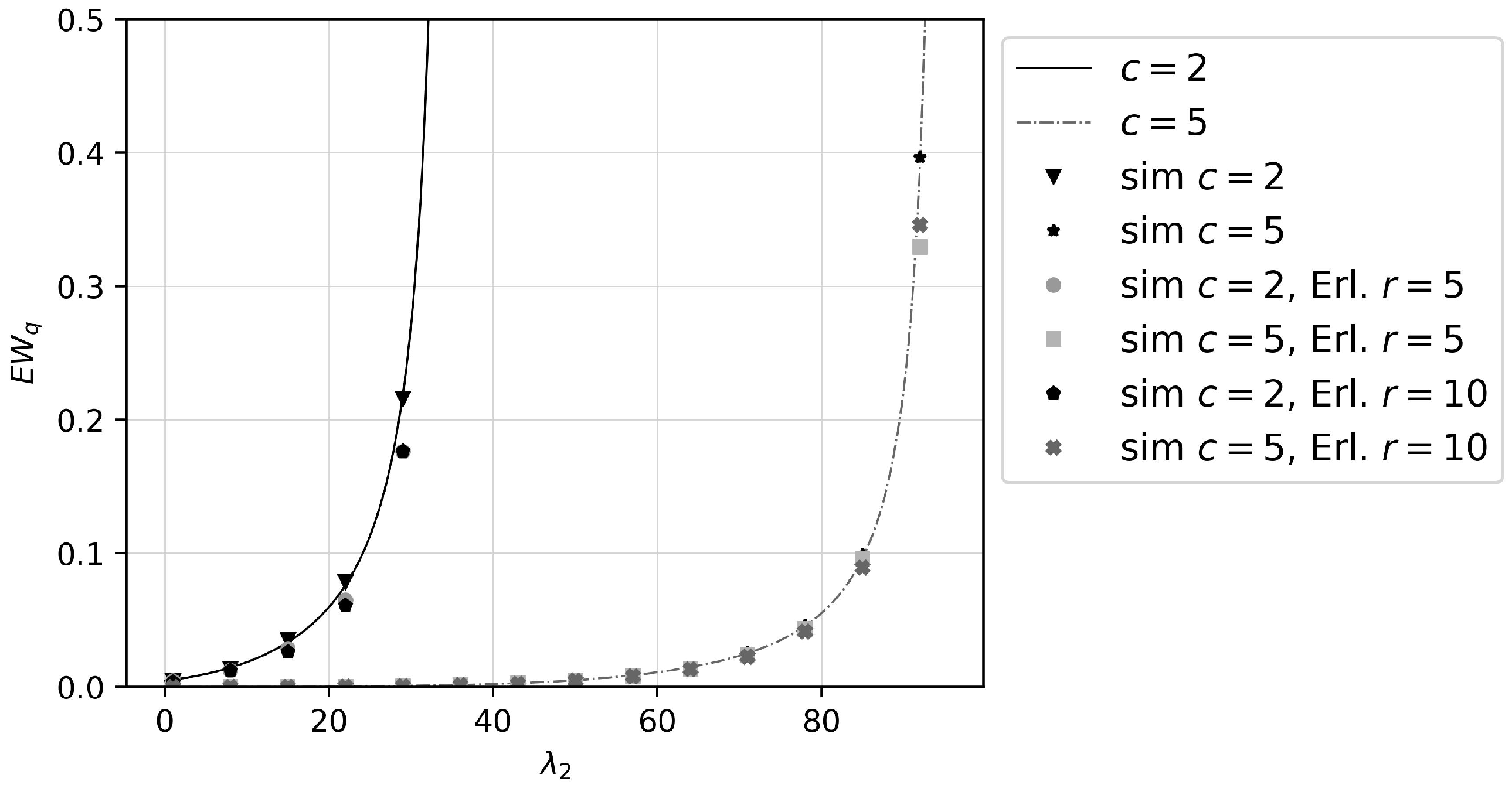
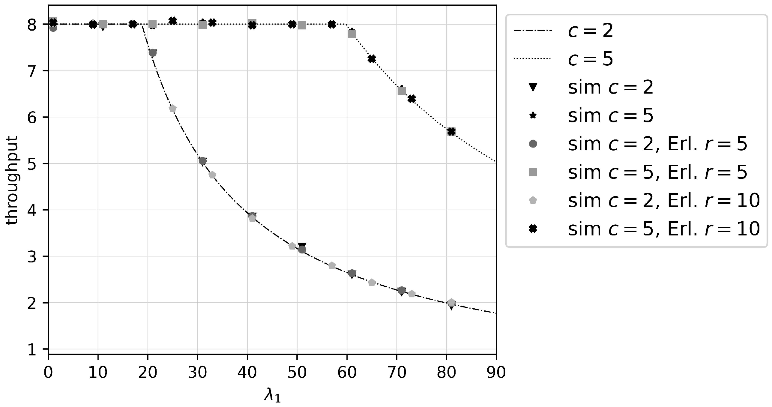
Figure 9 reflects changes in the throughput of class-2 customers against when is fixed. It can be seen that the throughput values remain unchanged at when goes up to certain thresholds; then, they drop as continues to increase. Meanwhile, Figure 10 indicates that the throughput is equal to up to a certain threshold of ; then, it remains unchanged at a value when class-2 customers arrive at very high rates. At that, equals the right-hand side of the stability condition (34).
Finally, it is noticeable that when we let the service times of class-1 customers follow Erlang distribution, the results do not change much as compared to the exponential case. This agrees with our stability condition, which depends on only the mean service time of class-1 customers.
7. Conclusions
In this paper, we have considered a modified Erlang system for cognitive radio networks and related applications. Using the regenerative methodology, we have established the stability condition, which is insensitive to the service time distributions of primary and secondary users. This analysis is sequentially considered for: (i) the system where there exists an infinite buffer for the awaiting secondary users, (ii) the system where the secondary users meeting a busy server join a virtual orbit and then make retrials and finally, (iii) the system where an idle server generates outgoing calls. The obtained results have implied that the throughput of secondary users is insensitive to the service time distributions of primary and secondary users, provided that the means are fixed. For the case of exponential service time distributions of primary and secondary customers, we have derived some stationary performance measures. Our extensive simulations have shown that the mean waiting time of secondary users increases with the increase in the variance of service time of primary users, while the mean number of terminations of secondary users is almost insensitive to the service time distributions of primary users, provided that the means are fixed. Our findings could be used in resource allocation in cognitive radio networks and related applications.
Author Contributions
Conceptualization, T.P.-D. and E.M.; methodology, T.P.-D., E.M., S.R. and H.Q.N.; software, H.Q.N.; validation, T.P.-D., E.M., S.R. and H.Q.N.; formal analysis, E.M., S.R., H.Q.N. and T.P.-D.; writing–original draft preparation, E.M., S.R., H.Q.N. and T.P.-D.; writing–review and editing, E.M., S.R., H.Q.N. and T.P.-D.; supervision, E.M. and T.P.-D. All authors have read and agreed to the published version of the manuscript.
Funding
The research of Hung Q. Nguyen was supported by JST SPRING, Grant Number JPMJSP2124. The research of Tuan Phung-Duc was supported by JSPS KAKENHI Grant Number 21K11765.
Institutional Review Board Statement
Not applicable.
Informed Consent Statement
Not applicable.
Data Availability Statement
Not applicable.
Conflicts of Interest
The authors declare no conflict of interest.
References
- Akyildiz, I.F.; Lee, W.Y.; Vuran, M.C.; Mohanty, S. NeXt generation dynamic spectrum access cognitive radio wireless networks: A survey. Comput. Netw. 2006, 50, 2127–2159. [Google Scholar] [CrossRef]
- Mitola, J.; Maguire, G.Q. Cognitive radio: Making software radios more personal. IEEE Pers. Commun. 1999, 6, 13–18. [Google Scholar] [CrossRef] [Green Version]
- Wang, B.; Liu, K.R. Advances in cognitive radio networks: A survey. IEEE J. Sel. Top. Signal Process. 2010, 5, 5–23. [Google Scholar] [CrossRef] [Green Version]
- Akyildiz, I.F.; Lee, W.Y.; Vuran, M.C.; Mohanty, S. A survey on spectrum management in cognitive radio networks. IEEE Commun. Mag. 2008, 46, 40–48. [Google Scholar] [CrossRef] [Green Version]
- Letaief, K.B.; Zhang, W. Cooperative communications for cognitive radio networks. Proc. IEEE 2009, 97, 878–893. [Google Scholar] [CrossRef] [Green Version]
- Ostovar, A.; Keshavarz, H.; Quan, Z. Cognitive radio networks for green wireless communications: An overview. Telecommun. Syst. 2021, 76, 129–138. [Google Scholar] [CrossRef]
- Mitrany, I.L.; Avi-Itzhak, B. A many-server queue with service interruptions. Oper. Res. 1968, 16, 628–638. [Google Scholar] [CrossRef]
- Akutsu, K.; Phung-Duc, T. Analysis of retrial queues for cognitive wireless networks with sensing time of secondary users. In Proceedings of the 14th International Conference, QTNA 2019, Ghent, Belgium, 27–29 August 2019; Springer: Cham, Switzerland, 2019; pp. 77–91. [Google Scholar]
- Phung-Duc, T.; Akutsu, K.; Kawanishi, K.; Salameh, O.; Wittevrongel, S. Annals of Operations Research. Perf. Eval. 2022, 310, 641–660. [Google Scholar]
- Salameh, O.; De Turck, K.; Bruneel, H.B.C.; Wittevrongel, S. Analysis of secondary user performance in cognitive radio networks with reactive spectrum handoff. Telecommun. Syst. 2017, 65, 539–550. [Google Scholar] [CrossRef] [Green Version]
- Salameh, O.; Bruneel, H.; Wittevrongel, S. Performance evaluation of cognitive radio networks with imperfect spectrum sensing and bursty primary user traffic. Math. Probl. Eng. 2020, 2020, 4102046. [Google Scholar] [CrossRef]
- Wong, E.W.A.; Foh, C.H. Analysis of cognitive radio spectrum access with finite user population. IEEE Wirel. Commun. Lett. 2009, 13, 294–296. [Google Scholar] [CrossRef]
- Konishi, Y.; Masuyama, H.; Kasahara, S.; Takahashi, Y. Performance analysis of dynamic spectrum handoff scheme with variable bandwidth demand of secondary users for cognitive radio networks. Wirel. Netw. 2013, 19, 607–617. [Google Scholar] [CrossRef]
- Shajin, D.; Dudin, A.N.; Dudina, O.; Krishnamoorthy, A. A two-priority single server retrial queue with additional items. J. Ind. Manag. Optim. 2020, 16, 2891–2912. [Google Scholar] [CrossRef]
- Zhang, Y.; Wang, J.; Li, W.W. Optimal pricing strategies in cognitive radio networks with heterogeneous secondary users and retrials. IEEE Access 2019, 7, 30937–30950. [Google Scholar] [CrossRef]
- Dudin, A.N.; Lee, M.H.; Dudina, O.; Lee, S.K. Analysis of priority retrial queue with many types of customers and servers reservation as a model of cognitive radio system. IEEE Trans. Commun. 2016, 65, 186–199. [Google Scholar] [CrossRef]
- Paul, S.; Phung-Duc, T. Retrial queueing model with two-way communication, unreliable server and resume of interrupted call for cognitive radio networks. In Information Technologies and Mathematical Modelling. Queueing Theory and Applications; Springer: Cham, Switzerland, 2018; pp. 213–224. [Google Scholar]
- Liu, J.; Jin, S.; Yue, W. Performance evaluation and system optimization of Green cognitive radio networks with a multiple-sleep mode. Ann. Oper. Res. 2019, 277, 371–391. [Google Scholar] [CrossRef]
- Nazarov, A.; Phung-Duc, T.; Paul, S. Unreliable single-server queue with two-Way communication and retrials of blocked and interrupted calls for cognitive radio networks. In Distributed Computer and Communication Networks; Springer: Cham, Switzerland, 2018; pp. 276–287. [Google Scholar]
- Dimitriou, I.; Phung-Duc, T. Analysis of cognitive radio networks with cooperative communication. In Proceedings of the 13th EAI International Conference on Performance Evaluation Methodologies and Tools, Tsukuba, Japan, 18–20 May 2020; pp. 192–195. [Google Scholar]
- Dragieva, V.I.; Phung-Duc, T. Unreliable single-server queue with two-Way communication and retrials of blocked and interrupted calls for cognitive radio networks. In Analytical and Stochastic Modelling Techniques and Applications; Springer: Cham, Switzerland, 2019; pp. 18–32. [Google Scholar]
- Kim, K. T-preemptive priority queue and its application to the analysis of an opportunistic spectrum access in cognitive radio networks. Comput. Oper. Res. 2012, 39, 1394–1401. [Google Scholar] [CrossRef]
- Azarfar, A.; Frigon, J.F.; Sanso, B. Priority queueing models for cognitive radio networks with traffic differentiation. EURASIP J Wirel. Commun. Netw. 2014, 2014, 206. [Google Scholar] [CrossRef] [Green Version]
- Neuts, M. Matrix Geometric Solutions in Stochastic Models—An Algorithmic Approach; Johns Hopkins University Press: Baltimore, MD, USA, 1981. [Google Scholar]
- Vishnevskiy, V.M.; Samouylov, K.E.; Yarkina, N.V. Mathematical model of LTE cells with machine-type and broadband communications. Autom. Remote Control 2020, 81, 622–636. [Google Scholar] [CrossRef]
- Asmussen, S. Applied Probability and Queues, 2nd ed.; Springer: New York, NY, USA, 2003. [Google Scholar]
- Morozov, E.; Steyaert, B. Stability Analysis of Regenerative Queueing Models; Springer: Cham, Switzerland, 2021. [Google Scholar]
- Morozov, E. Weak regeneration in modeling of queueing processes. Queueing Syst. 2004, 46, 295–315. [Google Scholar] [CrossRef]
- Feller, W. An Introduction to Probability Theory; Wiley: New York, NY, USA, 1971. [Google Scholar]
- Morozov, E. The tightness in the ergodic analysis of regenerative queueing processes. Queueing Syst. 1997, 27, 179–203. [Google Scholar] [CrossRef]
- Serfozo, R. Basics of Applied Stochastic Processes; Springer: Berlin/Heidelberg, Germany, 2009. [Google Scholar]
- Morozov, E.; Phung-Duc, T. Stability analysis of a multiclass retrial system with classical retrial policy. Perf. Eval. 2017, 112, 15–26. [Google Scholar] [CrossRef]
- Phung-Duc, T.; Masuyama, H.; Kasahara, S.; Takahashi, Y. A simple algorithm for the rate matrices of level-dependent QBD processes. In Proceedings of the 5th International Conference on Queueing Theory and Network Applications, Beijing, China, 24–26 July 2010; pp. 46–52. [Google Scholar]
Figure 1.
Construction in the system with 3 servers showing that .

Figure 2.
Average waiting time of class-2 customers against arrival rate of class-1 customers .

Figure 3.
Average waiting time of class-2 customers against arrival rate of class-2 customers ().

Figure 4.
Average number of waiting class-2 customers against arrival rate of class-1 customers .

Figure 5.
Average number of class-2 customers against arrival rate of class-2 customers ().

Figure 6.
Average number of termination events per class-2 customers against arrival rate of class-1 customers .
Figure 6.
Average number of termination events per class-2 customers against arrival rate of class-1 customers .

Figure 7.
Average number of termination events per class-2 customers against arrival rate of class-2 customers ().
Figure 7.
Average number of termination events per class-2 customers against arrival rate of class-2 customers ().

Figure 8.
Distribution of number of termination events ().

Figure 9.
Throughput against arrival rate of class-1 customers ().

Figure 10.
Throughput against arrival rate of class-2 customers ().

Publisher’s Note: MDPI stays neutral with regard to jurisdictional claims in published maps and institutional affiliations. |
© 2022 by the authors. Licensee MDPI, Basel, Switzerland. This article is an open access article distributed under the terms and conditions of the Creative Commons Attribution (CC BY) license (https://creativecommons.org/licenses/by/4.0/).
Share and Cite
MDPI and ACS Style
Morozov, E.; Rogozin, S.; Nguyen, H.Q.; Phung-Duc, T. Modified Erlang Loss System for Cognitive Wireless Networks. Mathematics 2022, 10, 2101. https://0-doi-org.brum.beds.ac.uk/10.3390/math10122101
AMA Style
Morozov E, Rogozin S, Nguyen HQ, Phung-Duc T. Modified Erlang Loss System for Cognitive Wireless Networks. Mathematics. 2022; 10(12):2101. https://0-doi-org.brum.beds.ac.uk/10.3390/math10122101
Chicago/Turabian StyleMorozov, Evsey, Stepan Rogozin, Hung Q. Nguyen, and Tuan Phung-Duc. 2022. "Modified Erlang Loss System for Cognitive Wireless Networks" Mathematics 10, no. 12: 2101. https://0-doi-org.brum.beds.ac.uk/10.3390/math10122101
Note that from the first issue of 2016, this journal uses article numbers instead of page numbers. See further details here.