A Novel Inverse Time–Frequency Domain Approach to Identify Random Forces

Abstract

In order to ensure the reliability and safety of complex engineering structures and allow their redesign and evaluation, the estimation of dynamic loads applied on them is vital. In this paper, a novel time–frequency domain approach is proposed to identify random forces based on the weighted regularization algorithm. Firstly, the Newmark’s algorithm was applied to obtain structural dynamic responses, then a weighed regularization algorithm was used to identify the random forces exerted on the engineering structure. The weighting matrix was used to control the identified error of the random forces. A spatial frame model was built to illustrate the practicality of the proposed approach. The experimental results demonstrated that the proposed method is more effective than other methods for random forces identification.

1. Introduction

In order to ensure the reliability and safety of complex engineering structures, the estimation of dynamic loads applied on them is very important and necessary. The information regarding dynamic loads is critical to the redesign and evaluation of these structures. However, in most cases, it is impractical to measure the dynamic loads directly, due to the many limitations of various operating environments. This occurs, for example, when measuring the impact load suffered by fighter aircrafts during taking off and landing on the deck, the buffeting loads of the vertical tail of aircrafts and the wind load acting on some high buildings. In these circumstances, it would be beneficial if the dynamic loads can be obtained by using the measured structural random response, which is relatively easy to acquire using some acceleration sensors. The study of the identification of dynamic load has a very high engineering application value.

The estimation of random forces is an inverse problem. Unfortunately, inverse problems are usually mathematically ill-posed. It means that a small change in the random response can lead to a big change in the force identification results [1]. To mitigate the challenges posed by the problem, J. O’Callahan et al. [2] used the singular value decomposition (SVD) approach to solve the ill-posed equation related to the inverse process of the system matrix, and the results showed that the regularization approach was very practical. The Tikhonov regularization method [3] is often used to solve ill-posed problems in many studies. Jia et al. [4,5] used measured frequency response functions to identify random forces considering the response error and model error. To improve the accuracy of their estimated results and reduce the impact of these errors, a weighted total least-square (TLS) method was applied. The feasibility and practically of the proposed method were validated by a random force estimation experiment. Jie Liu and Kun Li [6] used blind source separation and orthogonal matching pursuit to identify time–space-coupled distributed dynamic loads which were applied on a complicated structure. Their results demonstrated the validity of their proposed method. Batou and Soize [7,8] built a non-parametric probabilistic model to identify the random forces applied on a pressurized water reactor (PWR); good performance was obtained. Zhang et al. [9] proposed a Bayesian approach to identify dynamic forces, in relation to force identification on uncertain structures. Their results showed good performance of their method. Qiao feng Li and Qiu hai Lu [10] proposed a novel method to automatically identify a force history. Posterior distributions and uncertainties were also studied by a Metropolis-within-Gibbs sampler; a cantilever beam was used to validate the proposed method. Zhou et al. [11] used a deep recurrent neural network to identify the impact load applied to a nonlinear structure; the deep RNN model contained two LSTM layers and one bidirectional LSTM layer. The results of the comparison illustrated the validity of their proposed method. Feng et al. [12] proposed a new time domain regularization method to localize and reconstruct dynamic loads applied on structures based on structural dynamic responses. Liu et al. [13] proposed a novel method based on Artificial Neural Network (ANN) and Bayesian Probability framework (BPF) to identify dynamic forces; the interval model was applied to take into consideration some variables. The identified curve fit very well with the real curve, both in magnitude and in regularity. An augmented Kalman filter algorithm was tested by R. Cumbo [14] to identify dynamic loads; an existing optimal sensor placement strategy for Kalman Filter was also adopted. The effectiveness of the filter and the quality of the results demonstrated the validity of the proposed method. Tang [15] proposes a new method to identify loads based on the random response power spectral density and deep transfer learning strategy. This method is a data-driven model that can deal with ill-posed inverse problems in conventional methods. Onur Avci [16] described some highlights of the traditional methods and provided a comprehensive review of the most recent applications of the Machine Learning and Deep Learning algorithms used for vibration-based structural damage detection in civil structures. Hai Tran and Hirotsugu Inoue [17] proposed a wavelet deconvolution technique to identify impact forces by controlling the scale and shift components. Their results demonstrated the validity of their proposed method. A study [18] used the Bayesian approach to localize and estimate multiple dynamic loads in the time domain. Unknown dynamic loads were identified by the Markov chain Monte Carlo method with the Gibbs algorithm. In this paper, a novel inverse time–frequency domain approach is proposed, and the system matrix is also deduced. To solve the ill-posed equation, a weighted regularization approach was studied. The numerical example and experimental model were built to illustrate the performance of the proposed method.

The structure of this paper is as follows. The equations of motion of the structure and the system matrix are deduced, and the random responses are obtained by the Newmark’s method, as described in Section 2.1. In Section 2.2, a novel inverse time–frequency domain approach based on the weighed regularization algorithm is proposed. Section 3 verifies the proposed method by numerical simulation. In Section 4, an eight-storey spatial frame is studied to illustrate the practically of the proposed approach. Section 5 summarizes the conclusions.

2. Random Forces Identification

2.1. Equation of Motion

Consider an n degree-of-freedom (d. o. f) mechanical system, the equation of motion is as follows [19]:

$$M\ddot{y}\left(\mathrm{t}\right)+C\dot{y}\left(\mathrm{t}\right)+Ky\left(\mathrm{t}\right)=F\left(\mathrm{t}\right)$$

(1)

where $y\left(\mathrm{t}\right)\in {\mathrm{R}}^{\mathrm{n}\times 1}$ is the displacement vector, $M,C,K\in R^{\mathrm{n}\times \mathrm{n}}$ are the mass, damping and stiffness matrices, respectively, $F\left(\mathrm{t}\right)\in R^{\mathrm{n}\times 1}$ is the random force vector.

Introducing the state vector $x\left(\mathrm{t}\right)={\left[\mathrm{y}\left(\mathrm{t}\right),\dot{\mathrm{y}}\left(\mathrm{t}\right)\right]}^T$, Equation (1) can be rewritten as follows:

$$\dot{x}\left(\mathrm{t}\right)=A\mathrm{x}+BF\left(\mathrm{t}\right)$$

(2)

where

$$A=\left[\begin{array}{cc}\mathbf{0}& I\\ -M^{-1}K& -M^{-1}C\end{array}\right], B=\left[\begin{array}{c}\mathbf{0}\\ M^{-1}\end{array}\right]$$

The measured output vector $z\left(\mathrm{t}\right)$ is:

$$z\left(\mathrm{t}\right)=Cx\left(\mathrm{t}\right)+DF\left(\mathrm{t}\right)$$

(3)

where C and D are state matrices.

Equation (1) can be transformed into the following discrete equation:

$$x\left({\mathrm{t}}_{\mathrm{j}+1}\right)=A^{D}x\left({\mathrm{t}}_{\mathrm{j}}\right)+B^{D}F\left({\mathrm{t}}_{\mathrm{j}}\right)$$

(4)

where $A^D=\exp \left(A\Delta \mathrm{t}\right),B^D=A^{-1}\left(\exp \left(A\Delta \mathrm{t}\right)-I\right)B$.

Equation (3) can be formulated by the following discrete equation:

$$z\left(\mathrm{j}\right)=Cz\left(\mathrm{j}\right)+DF\left(\mathrm{j}\right)$$

(5)

Using the zero initial response of the engineering structure, the output vector can be expressed:

$$z\left(\mathrm{j}\right)=DF\left(\mathrm{j}\right)+{\displaystyle \sum }_{\mathrm{k}=1}^{\mathrm{j}}C{A}^{\mathrm{k}-1}BF\left(\mathrm{j}-\mathrm{k}\right)$$

(6)

let

$$H_{\mathrm{k}}=\{\begin{array}{c}D,\mathrm{k}=0\\ C{A}^{k-1}B,\mathrm{k}=1,\dots \mathrm{N}-1\end{array}$$

(7)

Equation (6) can be expressed in matrix form:

$$Z=\overline{H}F$$

(8)

where

$$\overline{H}=\left[\begin{array}{ccc}{H}_{\mathbf{0}}& \mathbf{0}& \begin{array}{cc}\mathbf{\cdots }& \mathbf{0}\end{array}\\ H_{\mathbf{1}}& H_{\mathbf{0}}& \begin{array}{cc}\mathbf{\cdots }& \mathbf{0}\end{array}\\ \begin{array}{c}\mathbf{⋮}\\ H_{N\mathbf{-}\mathbf{1}}\end{array}& \begin{array}{c}\mathbf{⋮}\\ H_{N\mathbf{-}\mathbf{2}}\end{array}& \begin{array}{cc}\begin{array}{c}\mathbf{\ddots }\\ \mathbf{\cdots }\end{array}& \begin{array}{c}\mathbf{⋮}\\ H_{\mathbf{0}}\end{array}\end{array}\end{array}\right], Z=\left[\begin{array}{c}{Z}_{\mathbf{0}}\\ Z_{\mathbf{1}}\\ \begin{array}{c}\mathbf{⋮}\\ Z_{N\mathbf{-}\mathbf{1}}\end{array}\end{array}\right], F=\left[\begin{array}{c}{F}_{\mathbf{0}}\\ F_{\mathbf{1}}\\ \begin{array}{c}\mathbf{⋮}\\ F_{N\mathbf{-}\mathbf{1}}\end{array}\end{array}\right]$$

To identify a random force, the random responses of the structure applied on the random loads are calculated by the Newmark’s $\mathsf{\beta }$ method. Considering the computational efficiency and computational speed, the constant average acceleration method was applied in this paper [20]. The random noise was added to the random responses to investigate its influence on the accuracy of the proposed method.

2.2. Random Forces Identification

To obtain the random forces $\mathrm{F}$, Equation (8) can be transformed into the following optimization problem

$$\min \Vert \overline{H}F-Z{\Vert }_2^2$$

(9)

The random forces can be calculated by:

$$F={\overline{H}}^{+}Z$$

(10)

where the superscript “+” denotes the Moore–Penrose pseudoinverse operator.

Because $Z$ and $\overline{H}$ contain some random noises, the identified dynamic loads from Equation (10) will have large deviations in some frequency Points. The identified error can be obtained:

$$\frac{\Vert \delta F{\Vert }_2}{\Vert F{\Vert }_2}\le k\left(\overline{H}\right)\frac{\Vert \delta Z{\Vert }_2}{\Vert Z{\Vert }_2}$$

(11)

To deal with this ill-posed problem, the weighted regularization method was adopted to control the identified error in this paper. Therefore, the ill-posed Equation (10) can be solved by the following optimization problem:

$$J_{\lambda }=\underset{\mathrm{F}}{\min }(\Vert \sqrt{W}\overline{H}F-\sqrt{W}{Z\Vert }^2+{\lambda }^2{\Vert F\Vert }^2)$$

(12)

where

$$W=\left[\begin{array}{c}\begin{array}{cc}\begin{array}{ccc}{w}_1& 0& \cdots \\ 0& w_2& 0\\ ⋮& \ddots & \ddots \end{array}& \begin{array}{c}0\\ 0\\ ⋮\end{array}\end{array}\\ \begin{array}{ccc}0& 0& \begin{array}{cc}0& w_N\end{array}\end{array}\end{array}\right]$$

To solve Equation (12), this optimization problem can be written as:

$$\underset{\mathrm{F}}{\min }\Vert \left[\begin{array}{c}\sqrt{W}\overline{H}\\ \lambda I\end{array}\right]F-{\left[\begin{array}{c}\sqrt{W}Z\\ 0\end{array}\right]\Vert }^2$$

(13)

where $\mathsf{\lambda }$ is a regularization parameter.

By simplifying Equation (13), we obtain

$$({\left(\sqrt{W}\overline{H}\right)}^{\mathrm{T}}\left(\sqrt{W}\overline{H}\right)+{\mathsf{\lambda }}^{2}I)F={\left(\sqrt{W}\overline{H}\right)}^{\mathrm{T}}\sqrt{W}Z$$

(14)

Through the approach of truncated singular value decomposition (TSVD), the matrix $\sqrt{W}\overline{H}$ can be turned into the following form:

$$\sqrt{W}\overline{H}=U\Sigma V^T$$

(15)

where $U$ and $V$ are orthogonal matrices, ${\sigma }_r\ge 0$ are singular values of the matrix $\sqrt{W}\overline{H}$, $\mathrm{r}$ is the rank of the matrix $\sqrt{W}\overline{H}$.

Substituting Equation (15) into Equation (14), the estimated random forces can be expressed in this form:

$$\widehat{F}=V{\Sigma }^{\prime }{U}^{\mathrm{T}}\sqrt{W}Z$$

(16)

where

$${\Sigma }^{\prime }=\left[\begin{array}{ccc}\frac{{\sigma }_1}{{\sigma }_{1 }^2+{\lambda }^2}& \cdots & \begin{array}{ccc}\cdots 0& \cdots & 0\end{array}\\ ⋮& \ddots & \begin{array}{ccc}0& ⋮& ⋮\end{array}\\ \begin{array}{c}0\\ ⋮\\ 0\end{array}& \begin{array}{c}0\\ ⋮\\ 0\end{array}& \begin{array}{ccc}\begin{array}{c}\frac{{\sigma }_i}{{\sigma }_{i }^2+{\lambda }^2}\\ ⋮\\ 0\end{array}& \begin{array}{c}0\\ \ddots \\ 0\end{array}& \begin{array}{c}0\\ ⋮\\ \frac{{\sigma }_r}{{\sigma }_{r }^2+{\lambda }^2}\end{array}\end{array}\end{array}\right]$$

(17)

According to the Fourier transform, the frequency domain random forces of the structure is obtained as follows [21]

$$\widehat{F}\left(\mathsf{\omega }\right)=V\left(\mathsf{\omega }\right){\Sigma }^{\prime }\left(\mathsf{\omega }\right)U^{\mathrm{T}}\left(\mathsf{\omega }\right)Z\left(\mathsf{\omega }\right)$$

(18)

According to the formula of power spectral density, the power spectral density matrix of random forces can be calculated by:

$$S_{FF}\left(\mathsf{\omega }\right)={\displaystyle \sum }_{\mathrm{i}=1}^{\mathrm{r}}\widehat{F_{\mathrm{i}}}\left(\mathsf{\omega }\right)\widehat{F_{\mathrm{i}}}{\left(\mathsf{\omega }\right)}^{\mathrm{T}}$$

(19)

The parameter $\mathsf{\lambda }$ in Equation (17) can be obtained by the Generalized Cross Validated GCV (GCV) method, and its optimal value can be achieved by obtaining the minimum value of the GCV function

$$\mathrm{G}\left(\mathsf{\lambda }\right)=\frac{\Vert \sqrt{W(}\overline{H}F-Z)\Vert }{\mathrm{tr}\left(\mathrm{I}-\sqrt{W}\overline{H}{\left({\overline{H}}^{\mathrm{T}}W\overline{H}+{\mathsf{\lambda }}^{2}I\right)}^{-1}{\overline{H}}^{\mathrm{T}}\sqrt{W}\right)}$$

(20)

where tr( ) denotes the matrix trace operator.

2.3. Summary of the Time–Frequency Method

In the above section, a novel inverse time–frequency domain approach based on the weighted regularization method was proposed. To better understand this approach, the algorithm can be briefly applied in these subsequent steps:

(1)

Obtain the random responses Z(t) by the Newmark’s $\mathsf{\beta }$ method.

(2)

Give the weighting matrix W and calculate the matrix $\sqrt{W}\overline{H}$.

(3)

Perform the truncated singular value decomposition of the matrix $\sqrt{W}\overline{H}$.

(4)

Select the proper regularization parameter $\mathsf{\lambda }$ by using the GCV function.

(5)

Compute the identified random forces $\widehat{F}\left(\mathsf{\omega }\right)$.

(6)

Obtain the PSD of the identified random forces $S_{FF}\left(\mathsf{\omega }\right)$

3. Numerical Validation

A five−layer frame model was built to demonstrate the proposed new method in this text, as shown in Figure 1. The structural parameters of the frame model were: modulus of elasticity E = 30 × 10⁹ N/m², modal damping ratio $\mathsf{\xi }=0.03$. The mass matrix and stiffness matrix of the frame structure are, respectively

$$M=144000\left[\begin{array}{ccc}1& 0& \begin{array}{cc}0& \begin{array}{cc}0& 0\end{array}\end{array}\\ 0& 1& \begin{array}{cc}0& \begin{array}{cc}0& 0\end{array}\end{array}\\ \begin{array}{c}0\\ 0\\ 0\end{array}& \begin{array}{c}0\\ 0\\ 0\end{array}& \begin{array}{cc}\begin{array}{c}1\\ 0\\ 0\end{array}& \begin{array}{c}\begin{array}{cc}0& 0\end{array}\\ \begin{array}{cc}1& 0\end{array}\\ \begin{array}{cc}0& 1\end{array}\end{array}\end{array}\end{array}\right]$$

(21)

$$K=2.0267\times {10}^8 \left[\begin{array}{ccc}2.9& -1.4& \begin{array}{cc}0& \begin{array}{cc}0& 0\end{array}\end{array}\\ -1.4& 2.7& \begin{array}{cc}-1.3& \begin{array}{cc}0& 0\end{array}\end{array}\\ \begin{array}{c}0\\ 0\\ 0\end{array}& \begin{array}{c}-1.3\\ 0\\ 0\end{array}& \begin{array}{cc}\begin{array}{c}2.5\\ -1.2\\ 0\end{array}& \begin{array}{c}\begin{array}{cc}-1.2& 0\end{array}\\ \begin{array}{cc}2.3& -1.1\end{array}\\ \begin{array}{cc}-1.1& 2.1\end{array}\end{array}\end{array}\end{array}\right]$$

(22)

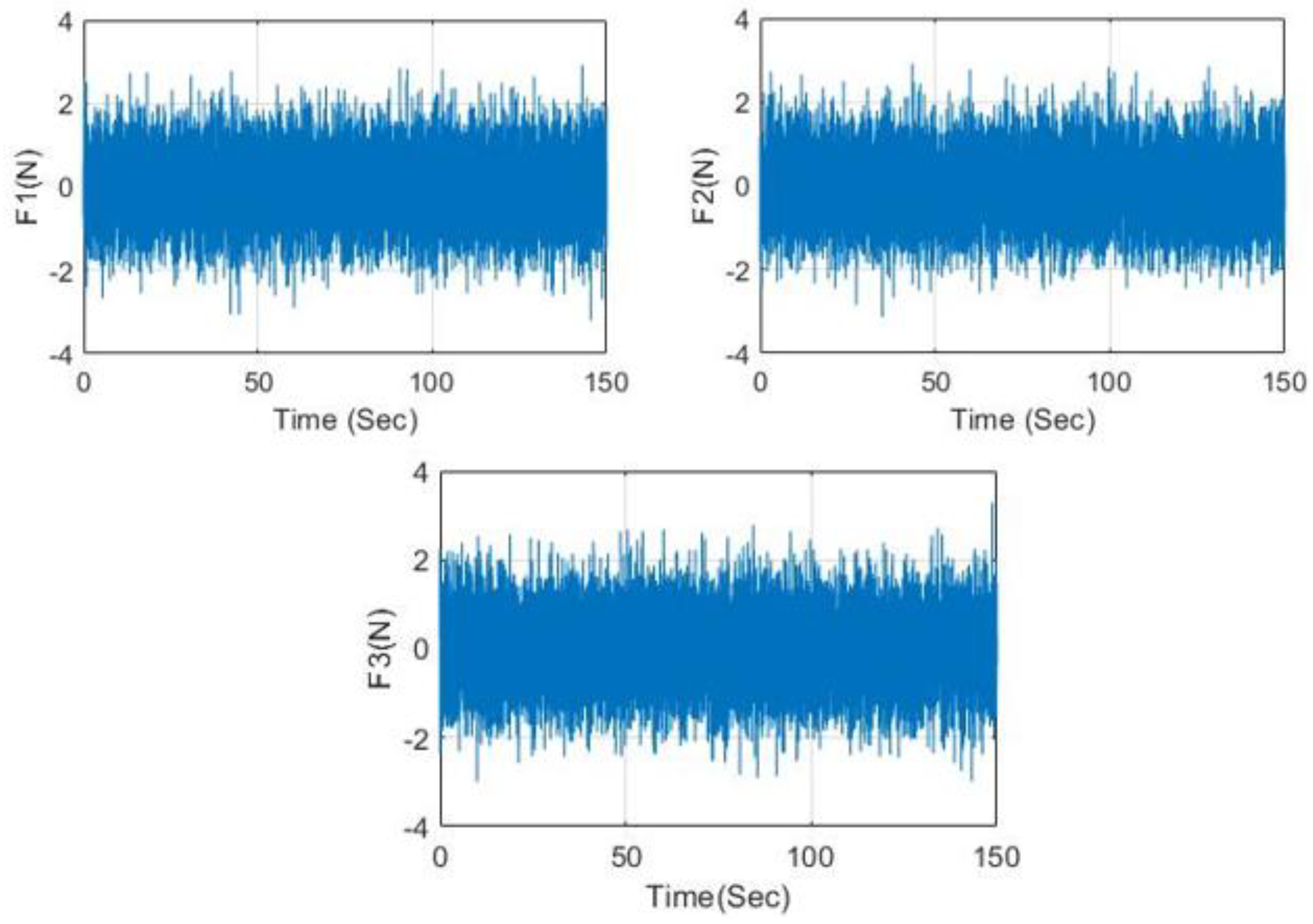
In order to obtain the structural dynamic responses, random forces were exerted on the 2nd, 3rd and 5th degree of freedom of the frame structure. The time histories of the exerted random forces are shown in Figure 1.

Assuming that the initial velocity and initial displacement of the frame model were set to zeros, the sampling step of the system was 0.01 s, and the sampling frequency was 100 Hz. In this section, the structural response (displacement responses and acceleration responses) were obtained by using the Newmark’s $\mathsf{\beta }$ = 0.25. The 5% random noise was also added into the random responses. The time histories of the displacement responses are shown in Figure 2.

In this approach, the weighted regularization method was adopted to identify the random forces applied on the five-layer frame model. Figure 3 shows a comparison between the actual random forces and the identified random forces. The two curves in Figure 3 show that the identified result and the actual result matched very well.

4. Experimental Verification

To illustrate the validity of the proposed inverse time–frequency domain method, an eight-degree-of-freedom frame structure was built in this study, as shown in Figure 4. According to the structural characteristics of the model, we assumed that the mass of each of its layers was concentrated on the layer spacer frames, while the stiffness was concentrated on the inter story columns. There were four pillars between two layers, and one pillar was made of three flat bars with a cross section of 0.139 m × 0.027 m × 0.001 m. Two electromagnetic exciters perpendicular to the frame structure were used to apply the random loads. Four response measurement points were selected on the frame to install acceleration sensors and obtain acceleration response signals during structural vibration. The frequency range in this experiment was 0–30 Hz, and the sampling frequency was 256 Hz. The experimentally measured the five acceleration random responses are shown in Figure 5.

To control the propagation of errors, the weighting matrix chosen for the experiments was

$$W=\left[\begin{array}{ccc}{\mathrm{w}}_1& & \\ & \ddots & \\ & & {\mathrm{w}}_6\end{array}\right]$$

(23)

where

$${\mathrm{w}}_{\mathrm{i}}=\sqrt{{\left({\displaystyle \sum }_{\mathrm{j}=1}^2{\left|{\overline{\mathrm{H}}}_{\mathrm{ij}}\right|}^2\right)}^{-1}}$$

(24)

According to the formula of power spectral density (PSD), the random response power spectral density can be obtained by using the time histories of four acceleration responses and the Fast Fourier Transform algorithm. Then, the PSDs of random forces can be determined.

As can be seen in Figure 6, the estimation errors of random forces were mainly concentrated around the natural frequency, especially within the range of 0–4 Hz. The main reasons of this were the random error of the random response and the system matrix error. To further illustrate the method, a comparison was made with a method described in reference [22]. The Root Mean Square (RMS) of the estimated random forces are presented in Table. From the data in the

Table 1. Estimated RMS results.

Method	Force 1	Force 2
Actual	0.5426	0.5662
Proposed method	0.6212	0.6108
method [22]	0.4587	0.4369

, the proposed time–frequency domain method appeared superior to the method presented in reference [22].

5. Conclusions

In this paper, a novel inverse time–frequency domain random force identification approach using the weighted regularization algorithms is proposed. The feasibility and practicality of the proposed method were verified by numerical simulations and experiments. Some concluding remarks can be drawn:

(1)

The results show that the time–frequency inverse method is able to correctly identify the random forces acting on engineering structures. It was also found that large errors mainly occurred at the beginning of the analysis.

(2)

The weighted regularization method can significantly improve the accuracy of load identification.

(3)

The format of the weighting matrix is not unique and can be optimized to improve the effectiveness of the method.

References

- Lee, H.; Park, Y. Error analysis of indirect force determination and a regularization method to reduce force determination error. Mech. Syst. Signal Process. 1995, 9, 615–633. [Google Scholar] [CrossRef]
- O’Callahan, J.; Piergentili, F. Force estimation using operational data. In Proceedings of the 14th International Modal Analysis Conference, Dearborn, MI, USA, 12–15 February 1995; SPIE: Bellingham, WA, USA, 1996; Volume 2768, pp. 1586–1592. [Google Scholar]
- Tikhonov, A.N.; Arsenin, V.Y. Solutions of Ill-Posed Problems, 1st ed.; Wiley: New York, NY, USA, 1977; pp. 84–102. [Google Scholar]
- Jia, Y.; Yang, Z.C.; Song, Q.Z. Experimental study of random dynamic loads identification based on weighted regularization method. J. Sound Vib. 2015, 342, 113–123. [Google Scholar] [CrossRef]
- Jia, Y.; Yang, Z.C.; Guo, N.; Wang, L. Random dynamic load identification based on error analysis and weighted total least squares method. J. Sound Vib. 2015, 358, 111–123. [Google Scholar] [CrossRef]
- Liu, J.; Li, K. Sparse identification of time-space coupled distributed dynamic load. Mech. Syst. Signal Process. 2021, 148, 107177. [Google Scholar] [CrossRef]
- Batou, A.; Soize, C. Identification of stochastic loads applied to a non-linear dynamical system using an uncertain computational model and experimental responses. Comput. Mech. 2009, 43, 559–571. [Google Scholar] [CrossRef]
- Batou, A.; Soize, C. Experimental identification of turbulent fluid forces applied to fuel assemblies using an uncertain model and fretting-wear estimation. Mech. Syst. Signal Process. 2009, 23, 2141–2153. [Google Scholar] [CrossRef] [Green Version]
- Zhang, E.; Antoni, J.; Feissel, P. Bayesian force reconstruction with an uncertain model. J. Sound Vib. 2012, 331, 798–814. [Google Scholar] [CrossRef]
- Li, Q.F.; Lu, Q.H. A hierarchical Bayesian method for vibration-based time domain force reconstruction problems. J. Sound Vib. 2018, 421, 190–204. [Google Scholar] [CrossRef]
- Zhou, J.M.; Dong, L.; Guan, W.; Yan, J. Impact load identification of nonlinear structures using deep recurrent neural network. Mech. Syst. Signal Process. 2019, 133, 106292. [Google Scholar] [CrossRef]
- Feng, W.; Li, Q.; Lu, Q.; Li, C.; Wang, B. Group relevance vector machine for sparse force localization and reconstruction. Mech. Syst. Signal Process. 2021, 161, 107900. [Google Scholar] [CrossRef]
- Liu, Y.; Wang, L.; Gu, K.; Li, M. Artificial Neural Network (ANN)—Bayesian Probability Framework (BPF) based method of dynamic force reconstruction under multi-source uncertainties. Knowl. Based Syst. 2022, 237, 107796. [Google Scholar] [CrossRef]
- Cumbo, R.; Tamarozzi, T.; Janssens, K.; Desmet, W. Kalman-based load identification and full-field estimation analysis on industrial test case. Mech. Syst. Signal Process. 2019, 117, 775–781. [Google Scholar] [CrossRef]
- Tang, Q.Z.; Xin, J.Z.; Jiang, Y.; Zhou, J.; Li, S. Novel identification technique of moving loads using the random response power spectral density and deep transfer learning. Measurement 2022, 195, 111120. [Google Scholar] [CrossRef]
- Avci, O.; Abdeljaber, O.; Kiranyaz, S.; Hussein, M.; Inman, D.J. A review of vibration-based damage detection in civil structures: From traditional methods to machine learning and deep learning applications. Mech. Syst. Signal Process. 2021, 147, 107077. [Google Scholar] [CrossRef]
- Tran, H.; Inoue, H. Further development and experimental verification of wavelet deconvolution technique for impact force reconstruction. Mech. Syst. Signal Process. 2021, 148, 107165. [Google Scholar] [CrossRef]
- Samagassi, S.; Jacquelin, E.; Khamlichi, A.; Sylla, M. Bayesian sparse regularization for multiple force identification and location in time domain. Inverse Probl. Sci. Eng. 2018, 27, 1221–1262. [Google Scholar] [CrossRef] [Green Version]
- Clough, R.W.; Penzien, J.; Griffin, D.S. Dynamics of structures. J. Appl. Mech. 1977, 44, 366. [Google Scholar] [CrossRef] [Green Version]
- Fan, Y.; Zhao, C.; Yu, H.; Wen, B. Dynamic load identification algorithm based on Newmark-β and self-filtering. Proc. Inst. Mech. Eng. Part C J. Mech. Eng. Sci. 2020, 234, 96–107. [Google Scholar]
- Bendat, J.; Piersol, A. Engineering applications of correlation and spectral analysis. J. Acoust. Soc. Am. 1998, 70, 262–263. [Google Scholar]
- Jia, Y.; Yang, Z.; Liu, E.; Fan, Y.; Yang, X. Prediction of random dynamic loads using second-order blind source identification algorithm. Proc. Inst. Mech. Eng. Part C J. Mech. Eng. Sci. 2020, 234, 1720–1732. [Google Scholar] [CrossRef]
Figure 1.
Random forces exerted on the structure.
Figure 2.
Calculated displacement responses.
Figure 3.
Estimation of the random forces. (a) Force 1; (b) force 2; (c) force 3.
Figure 4.
Experimental setup.
Figure 5.
Measured random acceleration responses.
Figure 6.
Comparison of estimated results and actual results: (a) force 1; (b) force 2.