
Speeding Up Semantic Instance Segmentation by Using Motion Information


Department of Computer Science and Engineering, Faculty of Automatic Control and Computer Engineering, “Gheorghe Asachi” Technical University of Iasi, D. Mangeron 27, 700050 Iasi, Romania
*
Author to whom correspondence should be addressed.
Mathematics 2022, 10(14), 2365; https://0-doi-org.brum.beds.ac.uk/10.3390/math10142365
Submission received: 14 June 2022
/
Revised: 1 July 2022
/
Accepted: 4 July 2022
/
Published: 6 July 2022
(This article belongs to the Special Issue Information Theory Applied in Scientific Computing)
Abstract
:Environment perception and understanding represent critical aspects in most computer vision systems and/or applications. State-of-the-art techniques to solve this vision task (e.g., semantic instance segmentation) require either dedicated hardware resources to run or a longer execution time. Generally, the main efforts were to improve the accuracy of these methods rather than make them faster. This paper presents a novel solution to speed up the semantic instance segmentation task. The solution combines two state-of-the-art methods from semantic instance segmentation and optical flow fields. To reduce the inference time, the proposed framework (i) runs the inference on every 5th frame, and (ii) for the remaining four frames, it uses the motion map computed by optical flow to warp the instance segmentation output. Using this strategy, the execution time is strongly reduced while preserving the accuracy at state-of-the-art levels. We evaluate our solution on two datasets using available benchmarks. Then, we conclude on the results obtained, highlighting the accuracy of the solution and the real-time operation capability.
Keywords:
machine vision; scene understanding; semantic instance segmentation; dense optical flow; real-timeMSC:
68T451. Introduction
The advances of the deep learning solutions led to a revolution in many fields. Computer vision benefited from this, and in recent years, many problems (e.g., image classification, object detection, semantic segmentation) have been solved by applying different deep learning techniques. Computer vision is present in a wide range of applications, from mobile robot navigation and industrial inspection to human–computer interaction (HCI), assistive devices, surveillance and autonomous driving.
Computer vision tries to replicate human vision by employing a great variety of solutions. Sight and vision represent two different aspects. Sight helps people acquire images from the environment, and on the other side, vision represents the process of interpreting these images (what happens in the brain). So, sight and vision help people to perceive and understand their surroundings. Thus, we can conclude that the goal of computer vision is to replicate human sight and vision by using a computer.
Environment perception and understanding is still a hot topic in this field, as solving this task means offering a solution to many real-world problems such as autonomous driving, scene perception and understanding for visually impaired, mobile robot navigation, surveillance and many others. Even if object detection and semantic segmentation held impressive results in the last decade, semantic instance segmentation remains an open challenge in the computer vision field. Many of the solutions proposed to solve this task focus on improving the accuracy of the method rather than achieving real-time processing. Therefore, they either require dedicated high-performance computing units to run or the inference is really slow, needing a high amount of time to perform the prediction.
In this paper, we present a novel framework for performing environment perception and understanding by semantic instance segmentation. The framework derived from [1], combines two computer vision tasks: semantic instance segmentation and dense optical flow, to achieve real-time operation capability while preserving the accuracy at state-of-the-art levels. The solution works by predicting the semantic instance labels and then propagating them by using the motion maps computed by employing dense optical flow.
We evaluate our solution on two datasets: the Cityscapes dataset [2] and our dataset, highlighting the real-time capability and the accuracy obtained.
2. Related Work
Our approach combines two computer vision tasks: semantic instance segmentation and optical flow. Therefore, this section is structured into two main parts. The first one depicts and compares various solutions for semantic instance segmentation focusing on the accuracy reported and on the inference time. In the second part, we present different methods for dense optical flow, highlighting their real-time operation capability.
2.1. Semantic Instance Segmentation
There is a clear difference between semantic segmentation and semantic instance segmentation. In semantic segmentation, every pixel of an image receives a class label (e.g., person, car, bicycle). In this case, there is no distinction between objects belonging to the same class. On the other hand, in semantic instance segmentation, objects of the same class are considered individual instances. So, semantic instance segmentation detects and localizes, at the pixel-level, objects instances in images. Even if impressive results have been reported for other segmentation techniques, semantic instance segmentation still represents one of the biggest challenges imposed by computer vision. There is a high interest in solving this task, as instance labelling provides additional information in comparison with semantic segmentation. Autonomous driving, medicine, assistive devices and surveillance are only a few applications in which semantic instance segmentation would represent a highly required input.
Instance segmentation solutions can be classified into one-stage and two-stage instance segmentation. Generally, the two-stage methods perform object detection, which is then followed by segmentation. Mask RCNN [3] extends [4] by adding a parallel branch to predict an object mask for the corresponding bounding box. Therefore, the loss function of Mask RCNN [3] combines the losses for bounding box, class recognition and mask segmentation. In addition, to improve the accuracy of the segmentation, RoI Pooling is replaced by RoI Align. MaskLab [5] is also built on top of the Faster RCNN [4] object detector. It combines semantic and direction prediction to achieve foreground/background segmentation. Semantic segmentation assists the model in distinguishing between objects of different semantic classes including background. On the other hand, direction prediction, which estimates each pixel’s direction toward its corresponding center, allows the separation of instances of the same semantic class. Hypercolumn features are exploited for mask refinement, and deformable crop and resize are used to improve the object detection branch. Huang et al. [6] proposed a framework that scores the instance segmentation mask. The score of the instance mask is penalized if it has a high classification score and the mask is not good enough. PANet [7] enhances the information flow in proposal-based solutions for semantic instance segmentation. A bottom–up path augmentation is added to enhance the extraction of the lower layers’ features. All feature levels are linked by adaptive feature pooling.
Even if the solution discussed above achieves state-of-the-art performance in terms of accuracy, the time needed for inference is rather high, which makes them unsuitable for integration in real-time systems.
One-stage methods usually perform detection and segmentation simultaneously. The authors of [8] use a fully convolutional network with two branches: one for estimating the segment instances and the other for scoring the instances. Each output pixel is a classifier of relative positions of instances which are further assembled using an instance assembling module. The first attempt for real-time instance segmentation was proposed in [9]. The instance segmentation is broken into two tasks: generating a set of prototype masks and predicting per-instance mask coefficients. The instance masks are produced by combining the prototype with the mask coefficients. Furthermore, in [10], deformable convolutions are added to the backbone, and the prediction head is optimized by using multi-scale anchors with different aspect ratios for each FPN level. The same idea as in Mask Scoring RCNN [6] is used to assign scores to the predicted masks.
Transformer-based networks were successfully applied in various computer vision tasks and held impressive results. Mask DINO [11] extends DINO [12] by adding a new branch to perform mask prediction for panoptic, instance and semantic segmentation. Content query embeddings from DINO [12] are used to perform mask classification for all segmentation tasks. QueryInst [13] proposes a query-based end-to-end instance segmentation with parallel supervision on six dynamic mask heads. QueryInst exploits the intrinsic one-to-one correspondence in queries across different stages. ISTR [14] matches low-dimensional mask embeddings with ground truth to compute the loss. In addition, it uses a recurrent refinement strategy to simultaneously perform detection and segmentation.
Image semantic and semantic instance segmentation, object detection and tracking, video object detection and segmentation, and video semantic segmentation have been well studied over time in comparison with video instance segmentation. This task implies the detection, segmentation and tracking of objects in a video sequence. Yang et al. [15] were the first to tackle the topic of video instance segmentation. Their works use the state-of-the-art method [3] for image instance segmentation. A new branch is added to Mask RCNN for tracking instances across video frames. The instances are stored in external memory and matched with objects in later frames. A similar solution to [15] is proposed in [16]; it predicts a basis mask and a set of coefficients to improve the segmentation quality. It achieves a better execution time than [15], as it is built on [17]. Another online method for video instance segmentation is proposed by Li et al. [18]. Inter-frame correlations are encoded by using a bottom–up framework equipped with a temporal context fusion module. An instance-level correspondence across adjacent frames, instance flow, is used for efficient and robust tracking among instances. A few works treat the video instance segmentation in offline mode [19,20,21]. These methods typically model the temporal information.
2.2. Dense Optical Flow
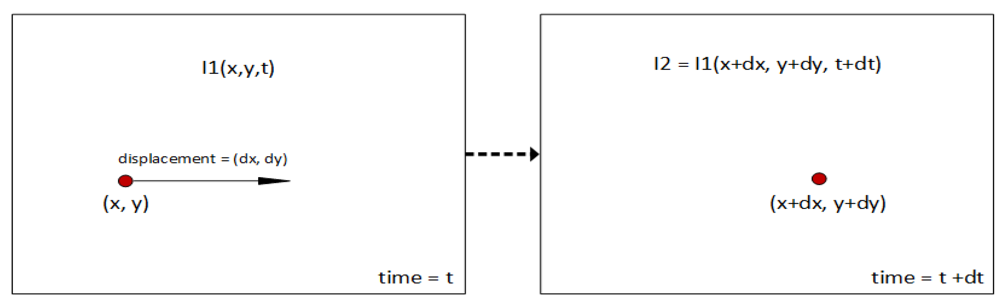
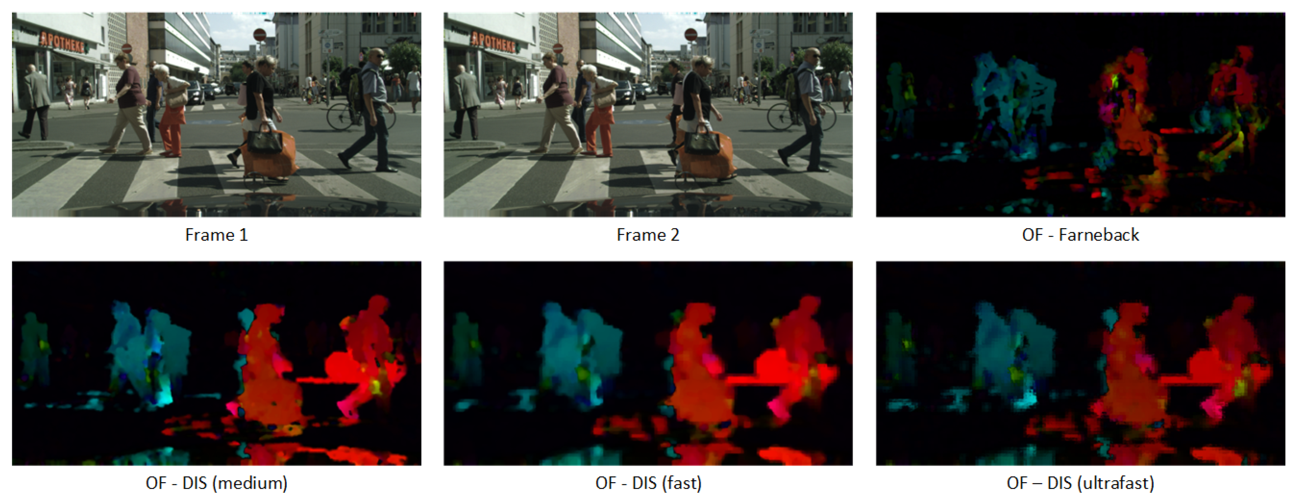
Optical flow represents the motion of objects between consecutive frames (Figure 1) and expresses the relative movement between objects and the camera.
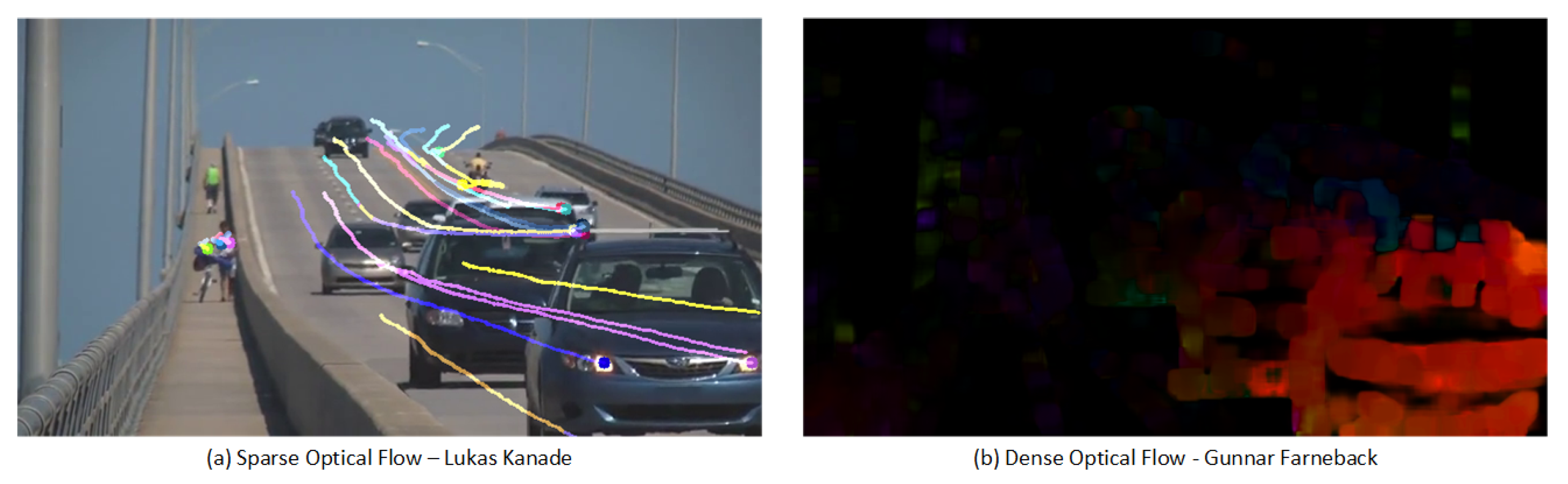
There are two types of optical flow: sparse optical flow and dense optical flow. Sparse optical flow describes the flow vector only for some objects’ features (e.g., edges, corners), while dense optical flow computes the flow vectors of all pixels from the image, as pictured in Figure 2.
The information provided by optical flow proves to be useful in a wide range of computer vision systems as well as in other applicative domains (e.g., action recognition, video compression, robots and vehicle navigation, video surveillance, fluid flow, etc.).
Horn and Schunck [22] and Lucas and Kanade [23] were the first authors to tackle the subject of optical flow more than three decades ago. Their patch-based approach uses a Taylor series expansion of the displaced image function to obtain sub-pixel estimates [23]. Horn and Schunck [22] proposed a regularization-based framework to simultaneously minimize the intensity between the corresponding pixels (over all flow vectors). The authors of [24] combine the ideas of [22,23] into a single framework that uses a locally aggregated Hessian as the brightness constancy term. Various techniques that use a combination of global and local motion were proposed [25,26,27,28].
Generally, the solutions published over time focused on improving the accuracy of the optical flow method rather than achieving real-time operation capability [29,30,31,32,33,34]. Some of the authors use powerful hardware resources to obtain an acceptable runtime [35,36], while others try to make a compromise between accuracy and time [37]. An efficient patch-based correspondence is proposed by Kroeger et al. in [38], which leads to a low computational time.
The fast evolution of deep neural networks led to their use in multiple computer vision problems, such as optical flow. DeepFlow [39] uses dense sampling to retrieve quasi-dense correspondences, which are further optimized using an energy variational framework. In [40] a classical spatial pyramid is combined with deep learning to estimate large motions. PWC-Net [41] computes a feature pyramid from each frame, warps the CNN features to the second image, and then builds a cost volume based on these two.
3. Method Description
The majority of the solutions proposed for semantic instance segmentation operate on single images. Deploying such methods in real-life applications is impractical as, generally, they require high execution time or dedicated hardware resources to operate in real-time. Video semantic instance segmentation represents a relatively new challenge in the computer vision field. Solving this task will open up the path to exploit semantic instance solutions in many applicative domains.
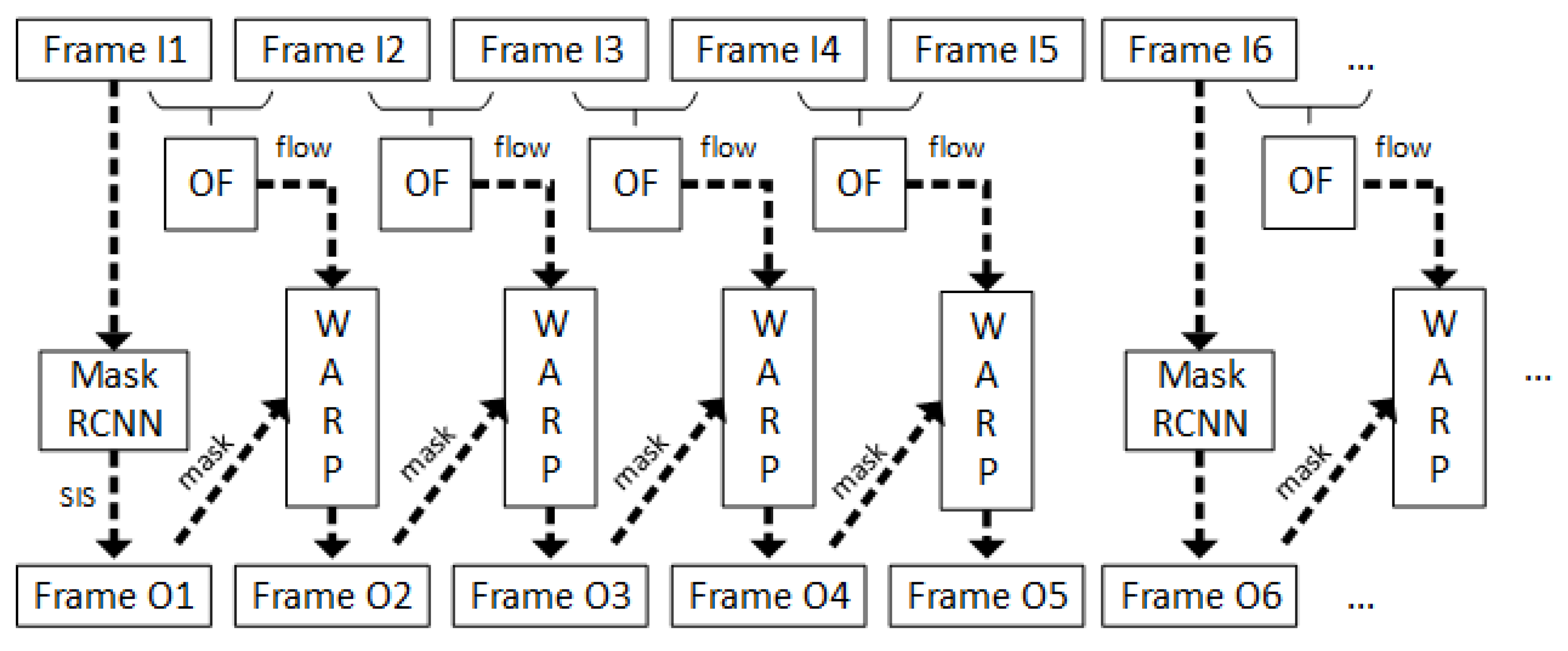
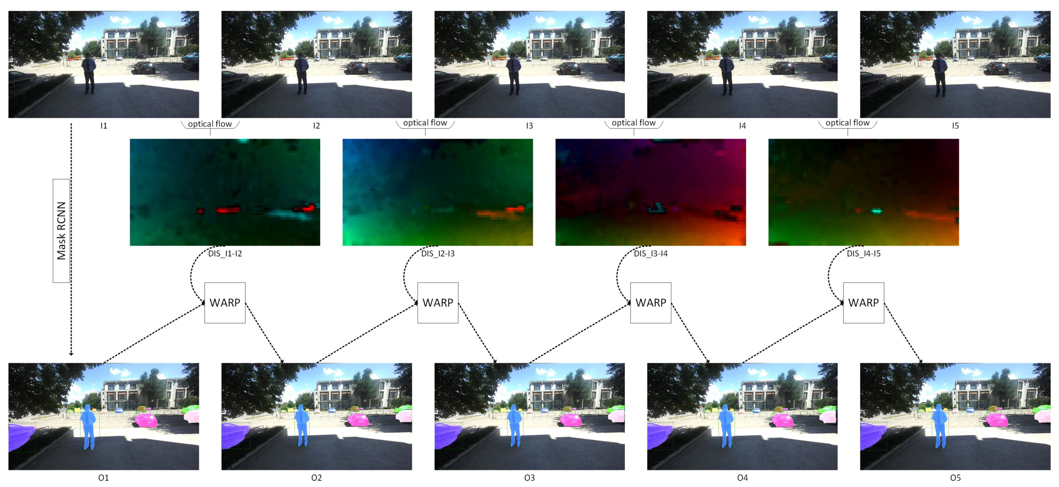
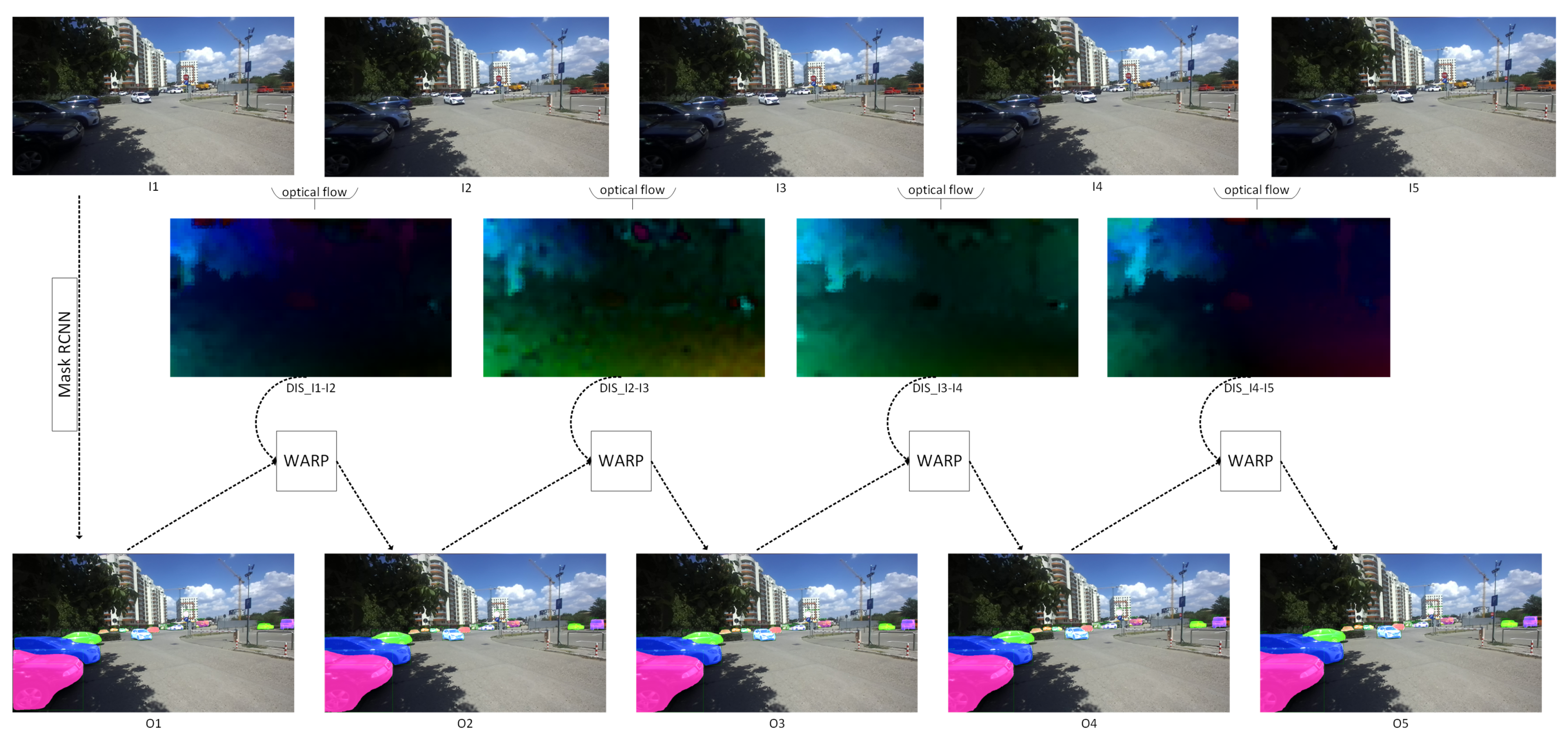
As stated above, using the Mask RCNN [3] to output the predictions for every frame from a video is unfeasible, as it will require a longer time to run. We propose a novel solution that combines the state-of-the-art solution for semantic instance segmentation, Mask RCNN [3], with a lightweight and powerful dense optical flow algorithm, DIS [38]. The solution is an adaptation of the framework proposed in [1] for speeding up the semantic segmentation task. The pipeline of our method is illustrated in Figure 3. Firstly, Mask RCNN [3] is used to output the instance labels for every fifth frame. Meanwhile, using the dense optical flow solution, we compute the motion map for every pixel from the current frame. Afterwards, the semantic labels obtained by employing the Mask RCNN solution are propagated into the next four frames by using the map calculated by dense optical flow, DIS [38].
For every pixel, , in the image, dense optical flow computes the flow for the two dimensions between two consecutive frames . Therefore, the mapping from to is:
Using Equation (1), pixels from frame will be remapped to frame as follows:
By using this strategy of combining two state-of-the-art methods, we succeeded in achieving real-time operation capability while maintaining the accuracy at state-of-the-art levels. In the following, we will describe the methods used, highlighting their advantages.
3.1. Mask RCNN
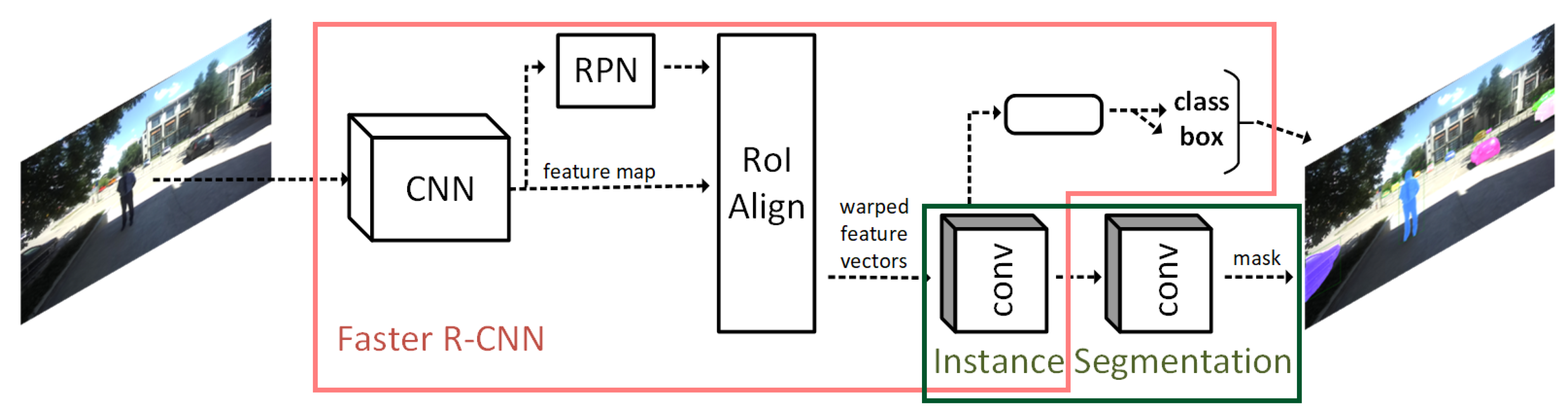
Mask RCNN [3] is an extension of the Faster RCNN network [4]. Faster RCNN is widely used for object detection tasks. For a given image as input, the outputs are the bounding box and the class label for each detected object in the image; Figure 4—red area. The Mask RCNN framework is developed on top of the Faster RCNN framework; Figure 4—green area. Therefore, for an image, besides the bounding box and the class label, the framework also returns the object mask for each detected object in the image.
Faster RCNN [4] is a two-stage object detector. First, a Region Proposal Network (RPN) is employed to generate candidate object bounding boxes. For these candidates, in the second stage, features are extracted using RoIPool. In the last step of the second stage, it performs classification and bounding-box regression. Mask RCNN inherits an identical (RPN) first stage from Faster RCNN. In the second stage, RoI Pooling is replaced by RoI Align, which leads to an improvement in the segmentation accuracy.
The network has another branch, the mask branch in parallel with the existing branch for classification and bounding-box regression, which outputs the segmentation mask for each region that contains an object and has an IoU above 0.5. The intersection over union (IoU) is an evaluation metric used to evaluate the accuracy of an object detector on a particular dataset and is computed as:
The authors of [3] mention that the framework proposed is not optimized for speed, claiming that their framework runs at around 200 ms (5 fps) per frame on an Nvidia Tesla M40 GPU.
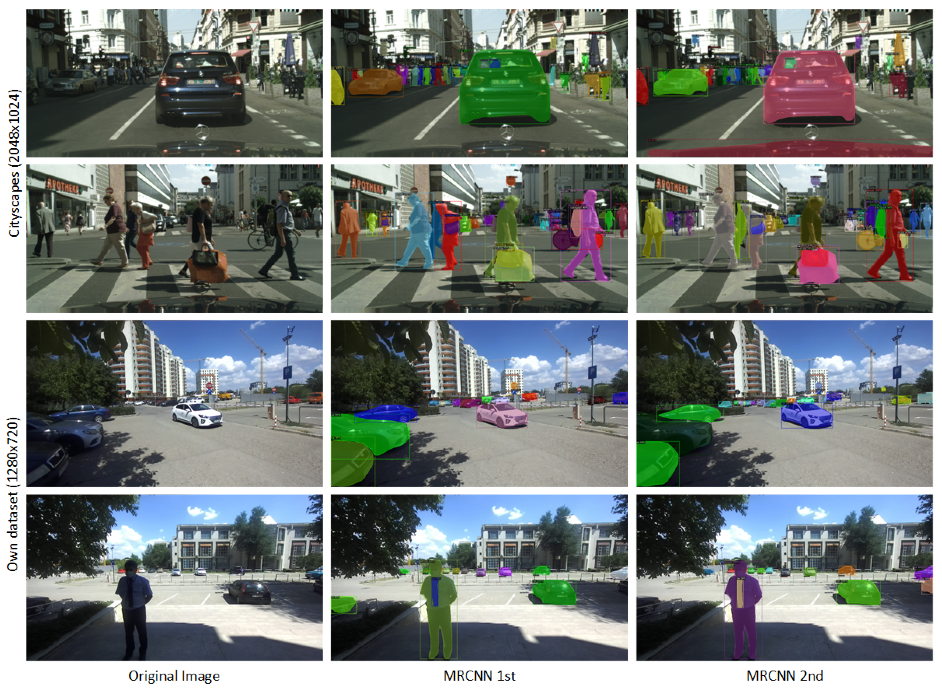
Some examples of predictions using Mask RCNN are presented in Figure 5.
Two pretrained models of the Mask RCNN neural network were used in the experiments: mask_rcnn_X_101_32x8d_FPN_3x and ask_rcnn_R_50_FPN_3x.
3.2. Dense Optical Flow
Dense optical flow computes the flow vectors of all pixels from the image. We have integrated two different solutions of dense optical flow into our framework.
3.2.1. Farneback Method
The Gunnar–Farneback algorithm was developed to produce dense optical flow technique results (that is, on a dense grid of points). The first step is to approximate each neighbourhood of both frames by quadratic polynomials. Afterwards, considering these quadratic polynomials, a new signal is constructed by a global displacement. Finally, this global displacement is calculated by equating the coefficients in the quadratic polynomials’ yields [43].
3.2.2. Dense Inverse Search
The computation of optical flow by using the Dense Inverse Search solution proposed in [38] consists of three main parts: the inverse search for patch correspondences, creating a dense displacement through path aggregation for multiple scales and variational refinement. The DIS [38] optical flow method has three configurable parameters that have a significant impact on the performance of the solution: finest scale, gradient descend iterations and patch size. DIS proposes three predefined values for each parameter. Therefore, there are three predefined versions of DIS: medium, fast and ultrafast; the values of the parameters are presented in Table 1.
As we can observe from Figure 6, the optical flow computation using the Farneback method has multiple regions with missing information.
4. Results
4.1. Datasets
Currently, there is no dataset that provides semantic instance labels for a full video sequence. The manual annotation task requires a lot of effort and attention to detail. These operations are generally executed by a person or a group of people. Such a dataset is hard to obtain through manual labelling.
4.1.1. Cityscapes Dataset
The Cityscapes dataset [2] contains stereo sequences recorded in street scenes from around 50 cities from Germany. The dataset contains high-resolution images (2048x1024). The dataset provides pixel-wise annotations for tasks such as semantic segmentation, semantic instance segmentation, and panoptic segmentation. A selection of frames from the frankfurt drive are already annotated for semantic instance segmentation and included in the val split of the Cityscapes dataset. Therefore, after running our algorithm, we have selected the results that correspond to the ground truth available in the val split. The accuracy is reported only on the selected results.
4.1.2. Own Dataset
The majority of the available datasets (Cityscapes [2], KITTI [44]) consist of images that are acquired from a car perspective. Unlike these datasets, the images available in our own dataset represent the perspective of a person, more exactly a visually impaired one. So, the environments are structurally dissimilar, as a person and a car have different routes to move in the cities. In addition, people can also move in indoor environments. We do not restrict the use of our algorithm to autonomous driving; therefore, we enlarge our evaluation and perform it also on our dataset. For this purpose, we use video sequences acquired in outdoor environments as we use the Cityscapes evaluation benchmark (which consists only of outdoor classes). Some examples of images from our dataset along with their annotations are displayed in Figure 5—last two rows. All the images are annotated using the best Mask RCNN pretrained model available. The dataset was acquired during the SoV Lite project [45].
4.2. Evaluation Metrics and Benchmarks
4.2.1. Benchmark
To evaluate the performance of our solution in terms of accuracy, we have used the benchmark provided by Cityscapes [2]. Therefore, we had to convert the results obtained by running the inference using Mask RCNN pretrained models to comply with the Cityscapes format. Considering that the pretrained models are trained on the COCO dataset [46], the evaluation was performed only on the common object classes from the two datasets: person, car, truck, bus, train, motorcycle, and bicycle.
4.2.2. Metrics
AP, AP50
To measure the performance of the instance-level segmentation, the Cityscapes [2] benchmark computes the average precision on the region level (AP) for each class. Afterwards, it averages it across a range of overlap thresholds (10 different overlaps from 0.5 to 0.95 with a step of 0.05 [47]) to avoid a bias toward a specific value. The overlap is calculated for every instance, making it equivalent to the intersection over union (IoU). Multiple predictions are penalized and marked as false positive (FP). The mean average precision (AP) reported is computed by averaging over the class label set and computed as follows:
where —represents the average precision of class k, which is computed at 10 different overlaps as:
and n represents the number of classes.
50 represents the average precision computed for an overlap of 0.5 as follows:
where —represents the average precision of class k computed for an overlap of 0.5 and n represents the number of classes.
Time
Another metric used to evaluate our solution is the execution time, as the proposed method is intended to be used in real-life applications. Thus, we measure the amount of time needed for every component of our pipeline. The evaluation is performed on two platforms with different configurations.
4.3. Results and Discussions
We used two pretrained Mask RCNN models [42]: mask_rcnn_X_101_32x8d_FPN_3x —best spretrained model (MRCNN 1st), mask_rcnn_R_50_FPN_3x—second best pretrained model (MRCNN 2nd), with the training configurations displayed in Table 2.
We also measure the performance of our solution by considering the depth information. Therefore, we evaluate our solution within 100, 50 and 25 m depth.
The evaluation is performed on two different platforms with the following configurations:
- Intel(R) Xeon(R) CPU @ 2.20 GHz, Tesla T4 GPU, 16 GB GPU memory; we will refer to this platform as Colab [49],
- Intel(R) Core(TM) i7-9700K CPU @ 3.60 GHz, Titan RTX GPU, 24 GB GPU memory; this platform will be referred to as RTX.
We highlight the real-time capability of our solution while maintaining the accuracy at state-of-the-art levels. In the next section, we will describe the experiments performed and discuss the results obtained. In the end, we compare our solution with other similar methods from the literature.
4.3.1. Accuracy
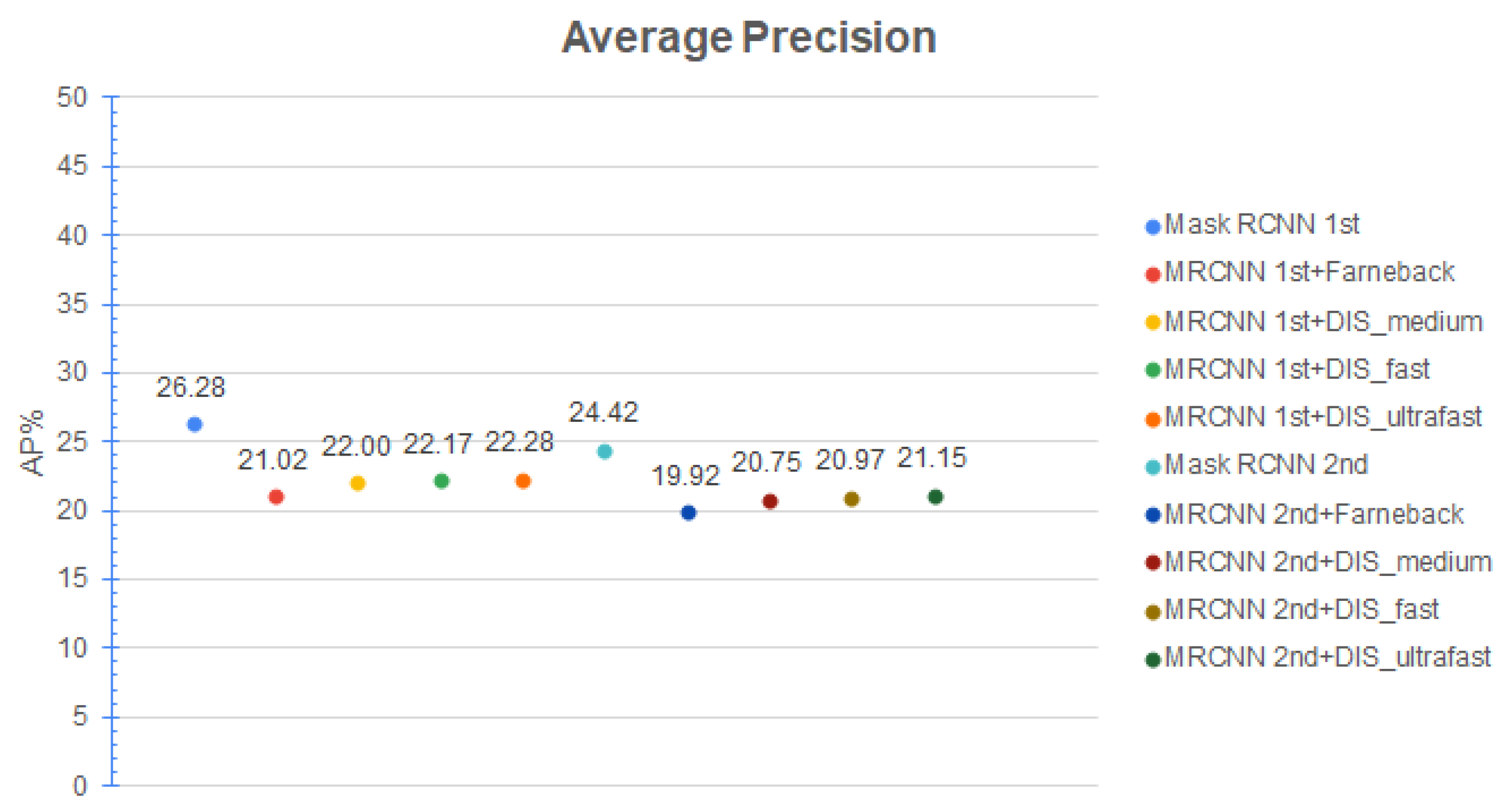
In the following, we evaluated the accuracy of our solution by using all three versions of DIS optical flow and also Farneback. In addition, we report the results for the two pretrained Mask RCNN models. The evaluation was performed using the val split of the Cityscapes dataset.
As illustrated in Figure 7, the pipeline using Mask RCNN combined with Farneback optical flow obtains the worst precision in terms of accuracy. The best combination is the Mask RCNN with DIS_ultrafast optical flow, which is followed immediately by DIS_fast. Comparing the Mask RCNN solution with our best result (Mask RCNN + DIS_ultrafast), the drop in accuracy is only 3–4%, which means that the accuracy is still preserved at state-of-the-art levels.
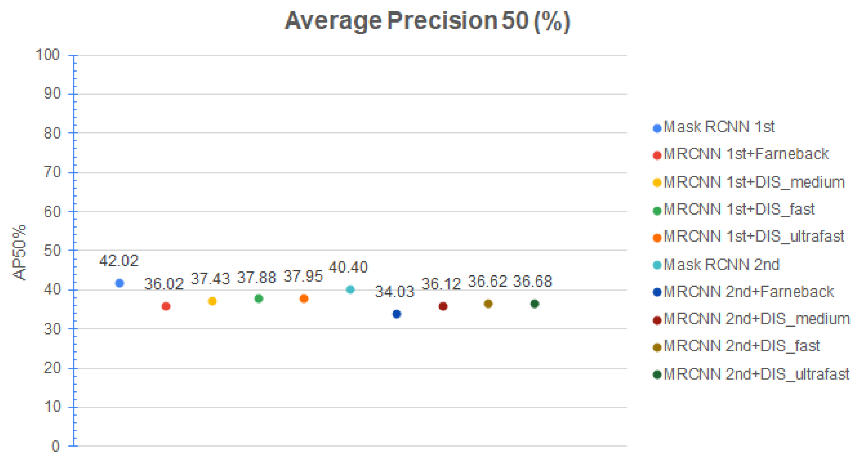
The same observations are available also for AP50. The only difference is that accuracy decreases only by 1–2%, as shown in Figure 8.
Depth Information
The farther the objects are located in the image, the less accurate the information extracted about them. Therefore, we restricted the range of the details to 100 m, 50 m and 25 m depth. Analyzing the results obtained for AP and AP50 from Table 3 and Table 4, we can conclude that the accuracy increases as the depth limit decreases. This trend is available for both the Mask RCNN and our proposed solution. In the case of our solution, the AP reaches a value of 37–38% and the AP50 reaches a value of 56% when limiting the information to 25 m depth. These results are beyond state-of-the-art solutions for semantic instance segmentation.
4.3.2. Time
The real-time requirement is critical in the context of intelligent mobile systems; therefore, we evaluated our proposed solution on all platforms mentioned before, highlighting their real-time operation capability.
Cityscapes Dataset
The Cityscapes dataset [2] contains high-resolution images pixels. The Mask RCNN [3] solution is built on top of Faster RCNN [4], which means that the image resolution has an impact on the inference time.
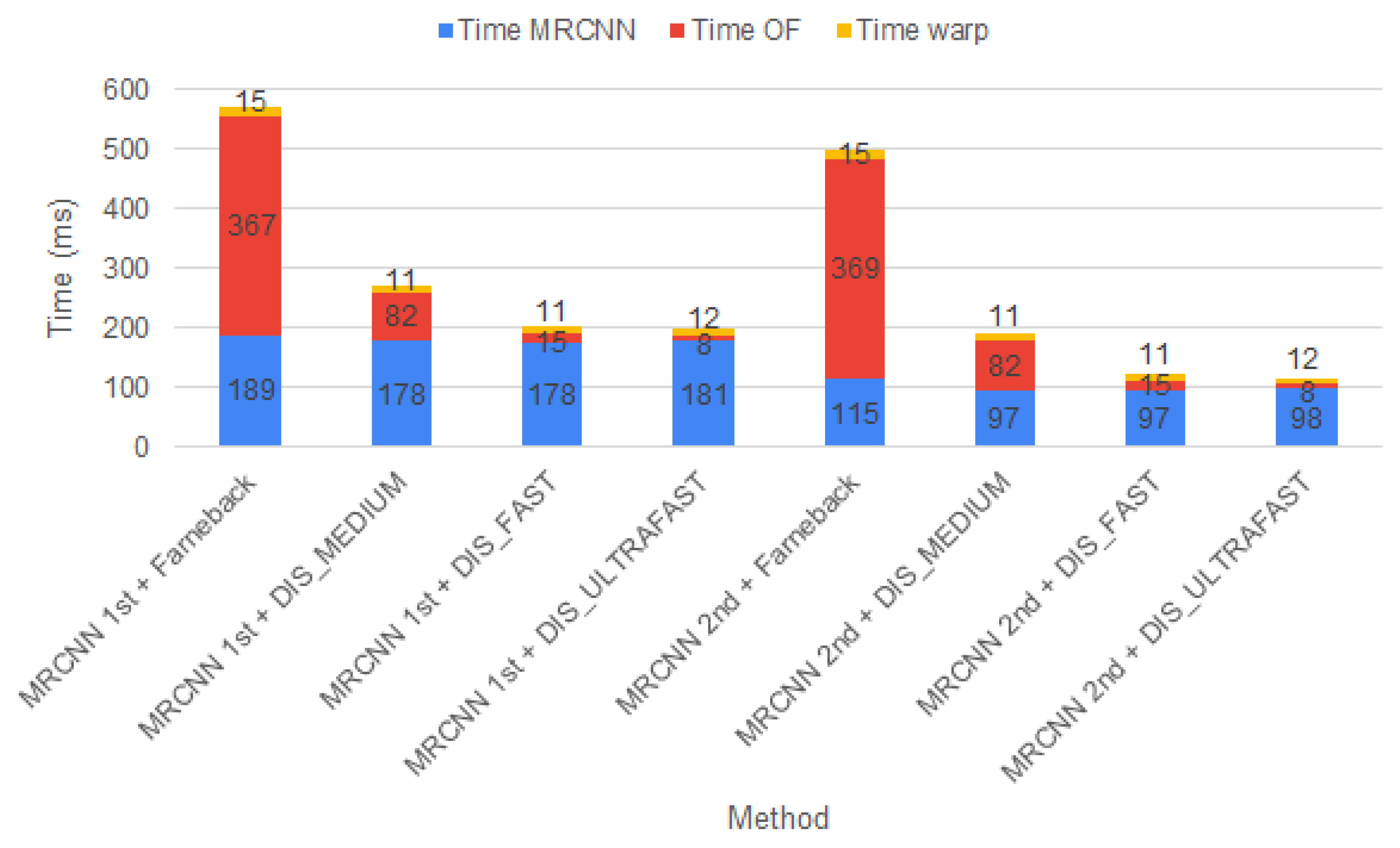
In Figure 9, we have illustrated the necessary time for all components of our pipeline. As we can observe, the inference time for the 2nd best model of Mask RCNN is two times smaller than the inference time of the 1st best model. It is also worth mentioning that the Farneback optical flow method requires about 370 ms to compute the motion map. The fastest method is represented by the combination of Mask RCNN with DIS_ULTRAFAST.
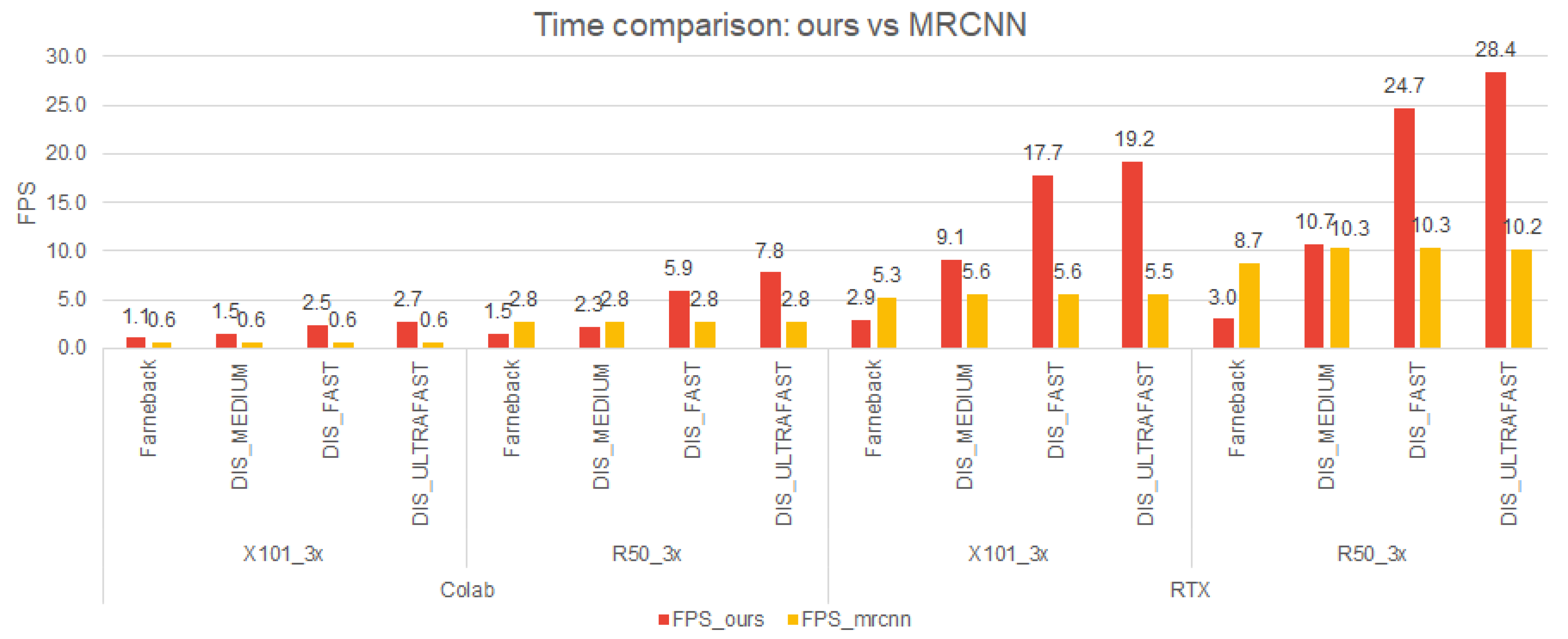
The total time necessary for our pipeline is presented for both platforms in Figure 10. Our best performing method (MRCNN 2nd + DIS_ULTRAFAST) is around three times faster than the corresponding Mask RCNN solution. The same trend is observed on both platforms. In addition, the RTX performs three times better than Colab. There are four situations in which the Mask RCNN solution outperforms the proposed pipeline: on Colab—MRCNN 2nd + Farneback and MRCNN 2nd + DIS_MEDIUM; on RTX—MRCNN 2nd + Farneback and MRCNN 1st + Farneback.
Our best solution formed with MRCNN 2nd + DIS_ULTRAFAST achieves about 8 fps on Colab and 28 fps on RTX; the pipeline is applied on high-resolution images ( pixels).
Own dataset
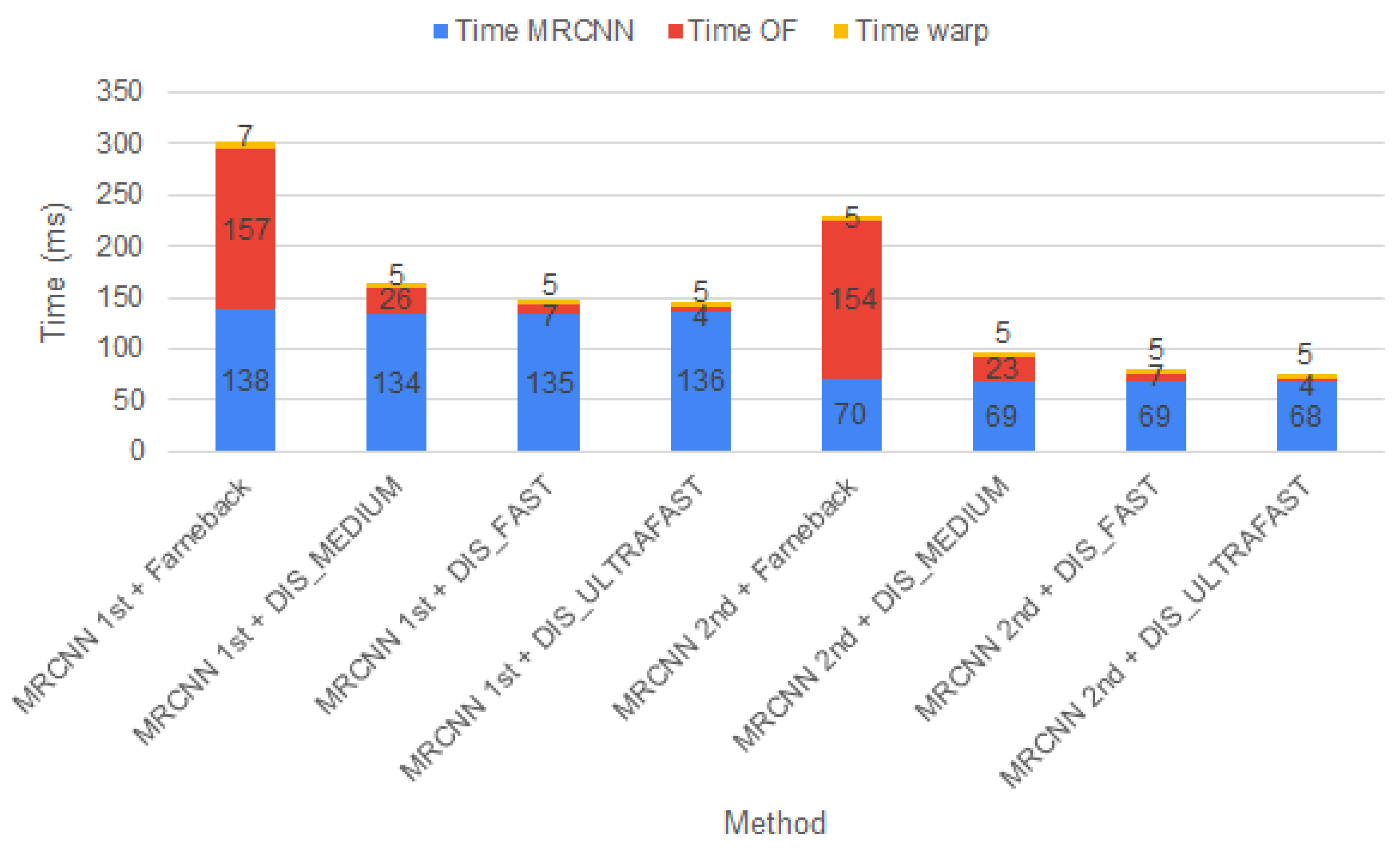
For our dataset, we have performed a similar evaluation. In this case, the image resolution is smaller, pixels, than the resolution of Cityscapes images. Therefore, the inference time for MRCNN 1st decreases by 50 ms, and for MRCNNnd, it decreases by 30 ms, as shown in Figure 11. The time needed for the optical flow methods as well as for warping the images is smaller compared with the time needed for the Cityscapes dataset. Farneback and DIS_MEDIUM optical flow solutions are three times faster when using our dataset. The other two optical flow methods (DIS_FAST and DIS_ULTRAFAST) are two times faster, and the time needed for warp is halved.
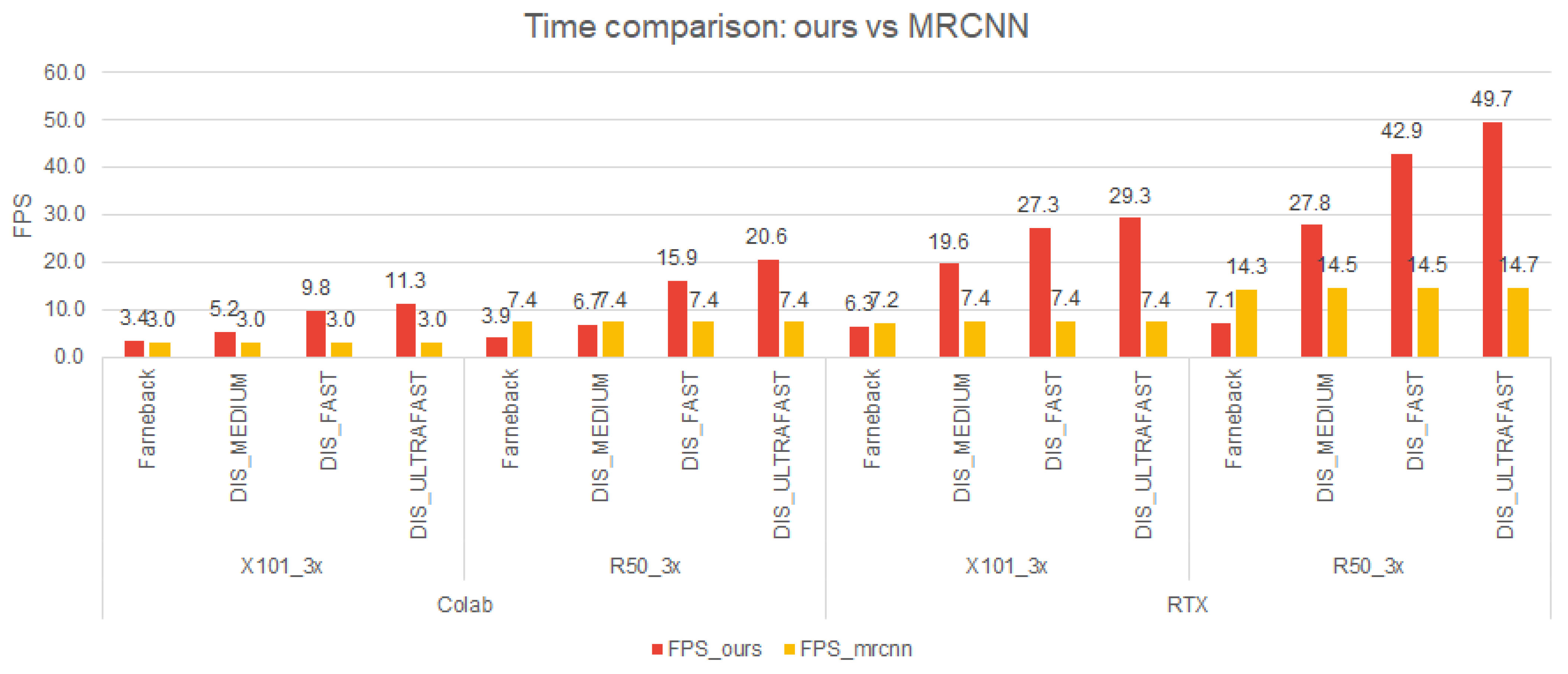
A similar trend as for the Cityscapes dataset [2] is observed for our dataset. The same four methods outperform our solution. Our best solution achieves 20 fps on Colab and around 50 fps on RTX for images with a pixels resolution, as shown in Figure 12. When comparing the two platforms, it is obvious that on RTX, our solution runs faster (about two times faster). It is also worth mentioning that for this particular resolution, MRCNN 1st + DIS_ULTRAFAST reaches real-time processing (almost 30 fps).
Concluding, the image resolution has a great impact on all components of our pipeline: MRCNN, OF and WARP. The lower the resolution, the faster the pipeline.
4.3.3. Frame Interval
As presented in Figure 3, our framework performs instance segmentation prediction on every 5th frame; afterwards, the output is propagated on the next four frames using the motion map. The selection of the frame interval was based on time evaluation. Table 5 illustrates the time of our solution obtained by varying the frame interval. The evaluation was performed on both datasets using the RTX platform.
From the results displayed in Table 5, we can observe that for high-resolution images (e.g., pixels), the real-time requirement is fulfilled by making predictions on every 5th frame and by using the MRCNN 2nd model for inference. For our dataset ( pixels), a frame interval of three frames is enough for real-time execution when using the MRCNN 2nd model. However, considering that the drop in accuracy is not high (only 3–4%), a frame interval of five frames can be used to achieve even a better time. In addition, it is worth mentioning the time improvement of our framework in contrast to the Mask RCNN solution.
4.3.4. Comparison with Other Solutions
We compared our solution with similar semantic instance segmentation solutions that report evaluation metrics on the Cityscapes dataset. The values for AP and AP50 are taken from the official Cityscapes (Cityscapes —https://www.cityscapes-dataset.com/, accessed on 1 July 2022) website or from their papers.
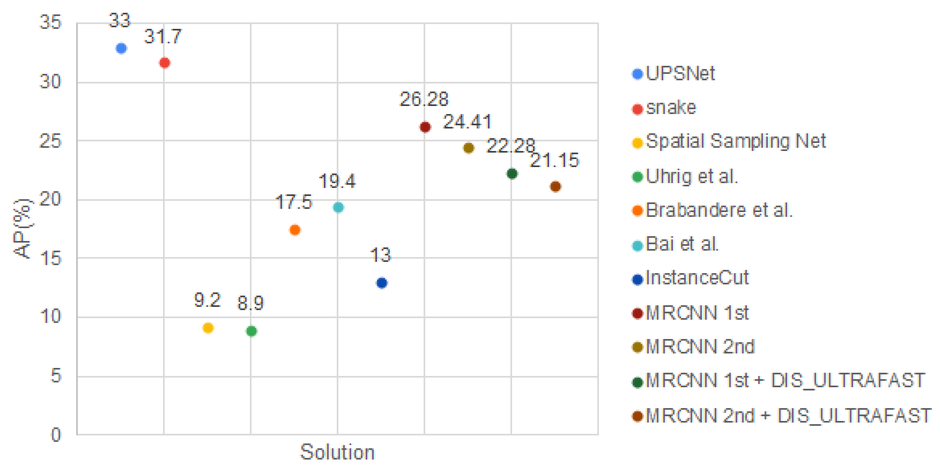
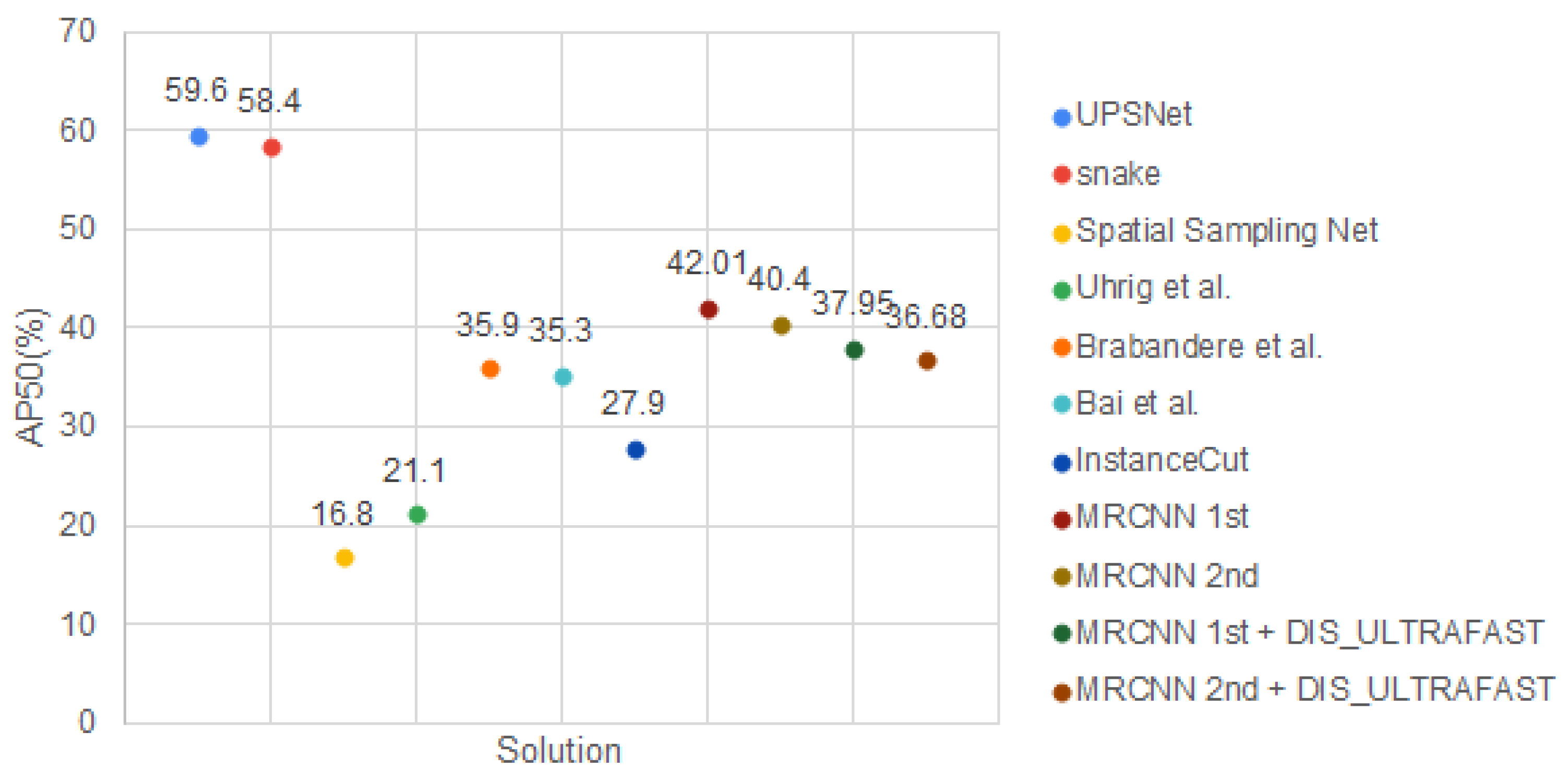
As we can observe, the Mask RCNN [3] pretrained model and the solutions proposed in [50,51] outperform our proposed solution. Even so, the other frameworks [52,53,54,55,56] perform worse than ours, some of them [52,53] two times worse, as shown in Figure 13. The same conclusions apply also on AP50%; see Figure 14.
Unfortunately, execution time is not available for all methods; therefore, we cannot perform a fair comparison between our solution and the other frameworks.
4.3.5. Discussions
To conclude, the best combination for our pipeline is formed with MRCNN 1st or 2nd and DIS_ULTRAFAST. There is only a 1% difference in AP between these solutions (MRCNN 1st + DIS_ULTRAFAST − 22.28% and MRCNN 2nd + DIS_ULTRAFAST − 21.15%), and the same is available also for 50. Even if the precision is almost similar for both solutions, the total time needed is different. For example, when using the Cityscapes dataset [2], MRCNN 1st + DIS_ULTRAFAST runs at 19 fps on RTX and 3 fps on Colab; meanwhile, MRCNN 2nd + DIS_ULTRAFAST reaches 28 fps on RTX and 8 fps on Colab. If our dataset is used, MRCNN 1st + DIS_ULTRAFAST achieves 29 fps RTX and 11 fps on Colab, while MRCNN 2nd + DIS_ULTRAFAST runs at 50 fps on RTX and 21 fps on Colab.
Therefore, the 1% drop in accuracy is insignificant if the solution is intended to be used in real-time applications, as the MRCNN 2nd + DIS_ULTRAFAST method is faster than the MRCNN 1st + DIS_ULTRAFAST. The results of the proposed solution are illustrated in Figure A1 and Figure A2. Mask RCNN 1st and DIS optical flow with ultrafast parameter were used.
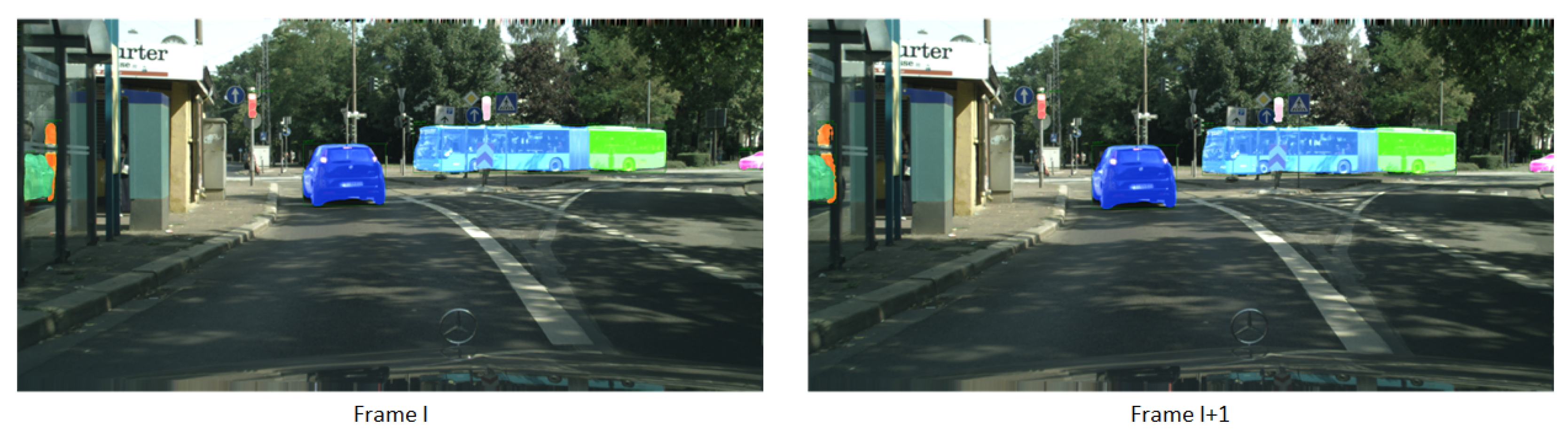
The performance of our solution is strongly dependent on the quality of the prediction. Thus, if the Mask RCNN solution output wrong predictions, these predictions will be propagated on another four frames. An example illustrating this situation is presented in Figure 15. As we can observe, there are multiple predictions for the same object (e.g., the bus), and those predictions are also propagated into the next frames.
5. Conclusions
In real-life applications, to output the semantic instance segmentation, we have to run the inference on every frame of the acquired video stream. Generally, semantic instance segmentation solutions available in the literature do not meet the real-time requirement, as they mainly focus on improving the accuracy of instance masks. The other solutions trade the accuracy to achieve real-time operation capability. Therefore, the two requirements—high accuracy and real-time processing—are often conflicting.
In this paper, we proposed and evaluated a novel solution for semantic instance segmentation. The solution is derived from [1]. The framework combines two state-of-the-art methods from semantic instance segmentation and optical flow fields. To reduce the time needed for performing inference on every frame, our framework runs the inference on every 5th frame and for the other four uses the computed motion map and warps the output of the semantic instance segmentation network. In this way, the time is strongly reduced, achieving in some cases even 50 fps on images with pixels resolution. Therefore, we can conclude that our framework is capable of outputting semantic instances in real-time. In addition, the accuracy of the solution increases if the information is limited to a specific range by using depth maps.
Author Contributions
Conceptualization, O.Z. and S.C. and V.-I.M.; methodology, O.Z.; software, O.Z.; validation, O.Z., S.C. and V.-I.M.; formal analysis, O.Z. and S.C. and V.-I.M.; investigation, O.Z.; resources, O.Z.; data curation, O.Z.; writing—original draft preparation, O.Z.; writing—review and editing, O.Z. and S.C. and V.-I.M.; visualization, O.Z.; supervision, S.C. and V.-I.M. All authors have read and agreed to the published version of the manuscript.
Funding
This research was funded by CNCS-UEFISCDI project PN-III-P2-2.1-PTE-2019-0810.
Institutional Review Board Statement
Not applicable.
Informed Consent Statement
Not applicable.
Data Availability Statement
Not applicable.
Conflicts of Interest
The authors declare no conflict of interest.
Abbreviations
The following abbreviations are used in this manuscript:
| MRCNN | Mask R-CNN |
| OF | Optical Flow |
| DOF | Dense Optical Flow |
| DIS | Dense Inverse Search |
| SIS | Semantic Instance Segmentation |
Appendix A. Results of the Proposed Solution on Our Dataset
Figure A1.
Framework results—our dataset (1): —input image x, —optical flow (DIS_ultrafast) between and , —output image (1).
Figure A1.
Framework results—our dataset (1): —input image x, —optical flow (DIS_ultrafast) between and , —output image (1).

Figure A2.
Framework results—our dataset (1): —input image x, _—optical flow (DIS_ultrafast) between and , —output image.
Figure A2.
Framework results—our dataset (1): —input image x, _—optical flow (DIS_ultrafast) between and , —output image.

References
- Paul, M.; Mayer, C.; Gool, L.V.; Timofte, R. Efficient Video Semantic Segmentation with Labels Propagation and Refinement. arXiv 2019, arXiv:1912.11844. [Google Scholar]
- Cordts, M.; Omran, M.; Ramos, S.; Rehfeld, T.; Enzweiler, M.; Benenson, R.; Franke, U.; Roth, S.; Schiele, B. The Cityscapes Dataset for Semantic Urban Scene Understanding. In Proceedings of the 2016 IEEE Conference on Computer Vision and Pattern Recognition (CVPR), Las Vegas, NV, USA, 27–30 June 2016; pp. 3213–3223. [Google Scholar] [CrossRef] [Green Version]
- He, K.; Gkioxari, G.; Dollár, P.; Girshick, R. Mask R-CNN. arXiv 2017, arXiv:1703.06870. [Google Scholar]
- Ren, S.; He, K.; Girshick, R.B.; Sun, J. Faster R-CNN: Towards Real-Time Object Detection with Region Proposal Networks. arXiv 2015, arXiv:1506.01497. [Google Scholar] [CrossRef] [Green Version]
- Chen, L.; Hermans, A.; Papandreou, G.; Schroff, F.; Wang, P.; Adam, H. MaskLab: Instance Segmentation by Refining Object Detection with Semantic and Direction Features. arXiv 2017, arXiv:1712.04837. [Google Scholar]
- Huang, Z.; Huang, L.; Gong, Y.; Huang, C.; Wang, X. Mask Scoring R-CNN. arXiv 2019, arXiv:1903.00241. [Google Scholar]
- Liu, S.; Qi, L.; Qin, H.; Shi, J.; Jia, J. Path Aggregation Network for Instance Segmentation. arXiv 2018, arXiv:1803.01534. [Google Scholar]
- Dai, J.; He, K.; Li, Y.; Ren, S.; Sun, J. Instance-sensitive Fully Convolutional Networks. arXiv 2016, arXiv:1603.08678. [Google Scholar]
- Bolya, D.; Zhou, C.; Xiao, F.; Lee, Y.J. YOLACT: Real-time Instance Segmentation. arXiv 2019, arXiv:1904.02689. [Google Scholar]
- Bolya, D.; Zhou, C.; Xiao, F.; Lee, Y.J. YOLACT++: Better Real-time Instance Segmentation. arXiv 2019, arXiv:1912.06218. [Google Scholar] [CrossRef]
- Li, F.; Zhang, H.; Xu, H.; Liu, S.; Zhang, L.; Ni, L.M.; Shum, H.Y. Mask DINO: Towards A Unified Transformer-based Framework for Object Detection and Segmentation. arXiv 2022, arXiv:2206.02777. [Google Scholar]
- Zhang, H.; Li, F.; Liu, S.; Zhang, L.; Su, H.; Zhu, J.; Ni, L.M.; Shum, H.Y. DINO: DETR with Improved DeNoising Anchor Boxes for End-to-End Object Detection. arXiv 2022, arXiv:2203.03605. [Google Scholar]
- Fang, Y.; Yang, S.; Wang, X.; Li, Y.; Fang, C.; Shan, Y.; Feng, B.; Liu, W. Instances as Queries. arXiv 2021, arXiv:2105.01928. [Google Scholar]
- Hu, J.; Cao, L.; Lu, Y.; Zhang, S.; Wang, Y.; Li, K.; Huang, F.; Shao, L.; Ji, R. ISTR: End-to-End Instance Segmentation with Transformers. arXiv 2021, arXiv:2105.00637. [Google Scholar]
- Yang, L.; Fan, Y.; Xu, N. Video Instance Segmentation. arXiv 2019, arXiv:1905.04804. [Google Scholar]
- Cao, J.; Anwer, R.M.; Cholakkal, H.; Khan, F.S.; Pang, Y.; Shao, L. SipMask: Spatial Information Preservation for Fast Image and Video Instance Segmentation. arXiv 2020, arXiv:2007.14772. [Google Scholar]
- Tian, Z.; Shen, C.; Chen, H.; He, T. FCOS: Fully Convolutional One-Stage Object Detection. arXiv 2019, arXiv:1904.01355. [Google Scholar]
- Li, X.; Wang, J.; Li, X.; Lu, Y. Video Instance Segmentation by Instance Flow Assembly. arXiv 2021, arXiv:2110.10599. [Google Scholar]
- Athar, A.; Mahadevan, S.; Osep, A.; Leal-Taixé, L.; Leibe, B. STEm-Seg: Spatio-temporal Embeddings for Instance Segmentation in Videos. arXiv 2020, arXiv:2003.08429. [Google Scholar]
- Bertasius, G.; Torresani, L. Classifying, Segmenting, and Tracking Object Instances in Video with Mask Propagation. arXiv 2019, arXiv:1912.04573. [Google Scholar]
- Wang, Y.; Xu, Z.; Wang, X.; Shen, C.; Cheng, B.; Shen, H.; Xia, H. End-to-End Video Instance Segmentation with Transformers. arXiv 2020, arXiv:2011.14503. [Google Scholar]
- Horn, B.K.; Schunck, B.G. Determining optical flow. Artif. Intell. 1981, 17, 185–203. [Google Scholar] [CrossRef] [Green Version]
- Lucas, B.D.; Kanade, T. An Iterative Image Registration Technique with an Application to Stereo Vision. In Proceedings of the 7th International Joint Conference on Artificial Intelligence—Volume 2, Vancouver, BC, Canada, 24–28 August 1981; Morgan Kaufmann Publishers Inc.: San Francisco, CA, USA, 1981. IJCAI’81. pp. 674–679. [Google Scholar]
- Bruhn, A.; Weickert, J.; Schnörr, C. Lucas/Kanade Meets Horn/Schunck: Combining Local and Global Optic Flow Methods. Int. J. Comput. Vis. 2005, 61, 211–231. [Google Scholar] [CrossRef] [Green Version]
- Adiv, G. Inherent ambiguities in recovering 3-D motion and structure from a noisy flow field. IEEE Trans. Pattern Anal. Mach. Intell. 1989, 11, 477–489. [Google Scholar] [CrossRef]
- Bergen, J.R.; Anandan, P.; Hanna, K.J.; Hingorani, R. Hierarchical model-based motion estimation. In Proceedings of the Computer Vision—ECCV’92, Santa Margherita Ligure, Italy, 19–22 May 1992; Sandini, G., Ed.; Springer: Berlin/Heidelberg, Germany, 1992; pp. 237–252. [Google Scholar]
- Szeliski, R.; Coughlan, J. Spline-Based Image Registration. Int. J. Comput. Vis. 1997, 22, 199–218. [Google Scholar] [CrossRef]
- Wedel, A.; Cremers, D.; Pock, T.; Bischof, H. Structure- and motion-adaptive regularization for high accuracy optic flow. In Proceedings of the 2009 IEEE 12th International Conference on Computer Vision, Kyoto, Japan, 27 September–4 October 2009; pp. 1663–1668. [Google Scholar] [CrossRef]
- Bailer, C.; Taetz, B.; Stricker, D. Flow Fields: Dense Correspondence Fields for Highly Accurate Large Displacement Optical Flow Estimation. IEEE Trans. Pattern Anal. Mach. Intell. 2019, 41, 1879–1892. [Google Scholar] [CrossRef] [PubMed] [Green Version]
- Bouguet, J.Y. Pyramidal Implementation of the Lucas Kanade Feature Tracker; Technical Report; Microprocessor Research Labs, Intel Corporation: Santa Clara, CA, USA, 2000. [Google Scholar]
- Fischer, P.; Dosovitskiy, A.; Ilg, E.; Häusser, P.; Hazirbas, C.; Golkov, V.; van der Smagt, P.; Cremers, D.; Brox, T. FlowNet: Learning Optical Flow with Convolutional Networks. arXiv 2015, arXiv:1504.06852. [Google Scholar]
- Leordeanu, M.; Zanfir, A.; Sminchisescu, C. Locally Affine Sparse-to-Dense Matching for Motion and Occlusion Estimation. In Proceedings of the 2013 IEEE International Conference on Computer Vision, Sydney, Australia, 1–8 December 2013; pp. 1721–1728. [Google Scholar] [CrossRef]
- Revaud, J.; Weinzaepfel, P.; Harchaoui, Z.; Schmid, C. EpicFlow: Edge-Preserving Interpolation of Correspondences for Optical Flow. arXiv 2015, arXiv:1501.02565. [Google Scholar]
- Timofte, R.; Van Gool, L. Sparse Flow: Sparse Matching for Small to Large Displacement Optical Flow. In Proceedings of the 2015 IEEE Winter Conference on Applications of Computer Vision, Waikoloa, HI, USA, 5–9 January 2015; pp. 1100–1106. [Google Scholar] [CrossRef]
- Bao, L.; Yang, Q.; Jin, H. Fast Edge-Preserving PatchMatch for Large Displacement Optical Flow. In Proceedings of the 2014 IEEE Conference on Computer Vision and Pattern Recognition, Columbus, OH, USA, 23–28 June 2014; pp. 3534–3541. [Google Scholar] [CrossRef]
- Plyer, A.; Besnerais, G.; Champagnat, F. Massively Parallel Lucas Kanade Optical Flow for Real-Time Video Processing Applications. J. Real-Time Image Process. 2016, 11, 713–730. [Google Scholar] [CrossRef]
- Wulff, J.; Black, M.J. Efficient sparse-to-dense optical flow estimation using a learned basis and layers. In Proceedings of the 2015 IEEE Conference on Computer Vision and Pattern Recognition (CVPR), Boston, MA, USA, 7–12 June 2015; pp. 120–130. [Google Scholar] [CrossRef]
- Kroeger, T.; Timofte, R.; Dai, D.; Gool, L.V. Fast Optical Flow using Dense Inverse Search. arXiv 2016, arXiv:1603.03590. [Google Scholar]
- Weinzaepfel, P.; Revaud, J.; Harchaoui, Z.; Schmid, C. DeepFlow: Large Displacement Optical Flow with Deep Matching. In Proceedings of the 2013 IEEE International Conference on Computer Vision, Sydney, Australia, 1–8 December 2013; pp. 1385–1392. [Google Scholar] [CrossRef] [Green Version]
- Ranjan, A.; Black, M.J. Optical Flow Estimation using a Spatial Pyramid Network. arXiv 2016, arXiv:1611.00850. [Google Scholar]
- Sun, D.; Yang, X.; Liu, M.; Kautz, J. PWC-Net: CNNs for Optical Flow Using Pyramid, Warping, and Cost Volume. arXiv 2017, arXiv:1709.02371. [Google Scholar]
- Wu, Y.; Kirillov, A.; Massa, F.; Lo, W.Y.; Girshick, R. Detectron2. 2019. Available online: https://github.com/facebookresearch/detectron2 (accessed on 1 July 2022).
- Suarez, O.D.; Fernández Carrobles, M.d.M.; Enano, N.V.; García, G.B.; Gracia, I.S. OpenCV Essentials; Packt Publishing: Birmingham, UK, 2014. [Google Scholar]
- Menze, M.; Geiger, A. Object Scene Flow for Autonomous Vehicles. In Proceedings of the Conference on Computer Vision and Pattern Recognition (CVPR), Boston, MA, USA, 7–12 June 2015. [Google Scholar]
- SoV Lite—Natural, Accessible and Ergonomic Audio-Haptic Sensory Substitution for the Visually Impaired. Available online: https://sovlite.eu/en/home-page/ (accessed on 4 June 2022).
- Lin, T.; Maire, M.; Belongie, S.J.; Bourdev, L.D.; Girshick, R.B.; Hays, J.; Perona, P.; Ramanan, D.; Dollár, P.; Zitnick, C.L. Microsoft COCO: Common Objects in Context. arXiv 2014, arXiv:1405.0312. [Google Scholar]
- Cityscapes Dataset-Benchmark Suite. Available online: https://www.cityscapes-dataset.com/benchmarks/#instance-level-scene-labeling-task (accessed on 4 June 2022).
- Deng, J.; Dong, W.; Socher, R.; Li, L.J.; Li, K.; Fei-Fei, L. Imagenet: A large-scale hierarchical image database. In Proceedings of the 2009 IEEE Conference on Computer Vision and Pattern Recognition, Miami, FL, USA, 20–25 June 2009; IEEE: Piscataway, NJ, USA, 2009; pp. 248–255. [Google Scholar]
- Google Colaboratory. Available online: https://colab.research.google.com/ (accessed on 4 June 2022).
- Xiong, Y.; Liao, R.; Zhao, H.; Hu, R.; Bai, M.; Yumer, E.; Urtasun, R. UPSNet: A Unified Panoptic Segmentation Network. arXiv 2019, arXiv:1901.03784. [Google Scholar]
- Peng, S.; Jiang, W.; Pi, H.; Bao, H.; Zhou, X. Deep Snake for Real-Time Instance Segmentation. arXiv 2020, arXiv:2001.01629. [Google Scholar]
- Mazzini, D.; Schettini, R. Spatial Sampling Network for Fast Scene Understanding. In Proceedings of the IEEE/CVF Conference on Computer Vision and Pattern Recognition (CVPR) Workshops, Long Beach, CA, USA, 15–20 June 2019. [Google Scholar]
- Uhrig, J.; Cordts, M.; Franke, U.; Brox, T. Pixel-level Encoding and Depth Layering for Instance-level Semantic Labeling. arXiv 2016, arXiv:1604.05096. [Google Scholar]
- Brabandere, B.D.; Neven, D.; Gool, L.V. Semantic Instance Segmentation with a Discriminative Loss Function. arXiv 2017, arXiv:1708.02551. [Google Scholar]
- Bai, M.; Urtasun, R. Deep Watershed Transform for Instance Segmentation. arXiv 2016, arXiv:1611.08303. [Google Scholar]
- Kirillov, A.; Levinkov, E.; Andres, B.; Savchynskyy, B.; Rother, C. InstanceCut: From Edges to Instances with MultiCut. arXiv 2016, arXiv:1611.08272. [Google Scholar]
Figure 1.
Optical Flow.

Figure 2.
Sparse Optical Flow vs. Dense Optical Flow. (a) Sparse Optical Flow-Lukas Kanade; (b) Dense Optical Flow-Gunnar Farneback.
Figure 2.
Sparse Optical Flow vs. Dense Optical Flow. (a) Sparse Optical Flow-Lukas Kanade; (b) Dense Optical Flow-Gunnar Farneback.

Figure 3.
Semantic instance segmentation pipeline, where —input frame i, —semantic instance segmentation output for frame i, —Optical Flow method, —image warping, and —semantic instance segmentation neural network [3].
Figure 3.
Semantic instance segmentation pipeline, where —input frame i, —semantic instance segmentation output for frame i, —Optical Flow method, —image warping, and —semantic instance segmentation neural network [3].

Figure 4.
Mask RCNN framework for instance segmentation [3]; Mask RCNN is built on top of Faster RCNN [4] adding another branch for mask prediction. RoI Pool is replaced with RoI Align.

Figure 5.
Mask RCNN output prediction examples on Cityscapes and our own images, MRCNN 1st—mask_rcnn_X_101_32x8d_FPN_3x, MRCNN 2nd—mask_rcnn_R_50_FPN_3x [42].
Figure 5.
Mask RCNN output prediction examples on Cityscapes and our own images, MRCNN 1st—mask_rcnn_X_101_32x8d_FPN_3x, MRCNN 2nd—mask_rcnn_R_50_FPN_3x [42].

Figure 6.
Optical Flow Examples.

Figure 7.
Average Precision, Cityscapes dataset [2].
Figure 7.
Average Precision, Cityscapes dataset [2].

Figure 8.
Average Precision (50%), Cityscapes dataset [2].
Figure 8.
Average Precision (50%), Cityscapes dataset [2].

Figure 9.
Mask RCNN, Optical Flow and Warp time, Cityscapes dataset [2], Colab platform.
Figure 9.
Mask RCNN, Optical Flow and Warp time, Cityscapes dataset [2], Colab platform.

Figure 10.
Time—Cityscapes dataset [2], RTX and Colab platforms.
Figure 10.
Time—Cityscapes dataset [2], RTX and Colab platforms.

Figure 11.
Mask RCNN, Optical Flow and Warp time, own dataset.

Figure 12.
Time—Own dataset, RTX and Colab platforms.

Figure 13.
Comparison between our framework and other solutions (AP%), Cityscapes dataset [2].
Figure 13.
Comparison between our framework and other solutions (AP%), Cityscapes dataset [2].

Figure 14.
Comparison between our framework and other solutions (AP50%), Cityscapes dataset [2].
Figure 14.
Comparison between our framework and other solutions (AP50%), Cityscapes dataset [2].

Figure 15.
Wrong predictions propagation on the next frame: Mask RCNN prediction for Frame I, label and mask propagation using DIS for Frame I+1.
Figure 15.
Wrong predictions propagation on the next frame: Mask RCNN prediction for Frame I, label and mask propagation using DIS for Frame I+1.


Table 1.
Dense Inverse Search predefined parameters values.
| Parameter | DIS_MEDIUM | DIS_FAST | DIS_ULTRAFAST |
|---|---|---|---|
| finest scale | 1 | 2 | 2 |
| gradient descend interations | 25 | 16 | 12 |
| patch size | 8 | 8 | 8 |
Table 2.
Models training configurations [42].
Table 2.
Models training configurations [42].
| Model | Pretrained Weights | Optimizer | Base Learning Rate | Learning Rate Scheduler |
|---|---|---|---|---|
| MRCNN 1st | ImageNet (X-101-32x8d.pkl) [48] | SGD | 0.02 | 3x |
| MRCNN 2nd | ImageNet (R-50.pkl) [48] | SGD | 0.02 | 3x |
Table 3.
Depth influence on , Cityscapes dataset [2].
Table 3.
Depth influence on , Cityscapes dataset [2].
| Model | Infinity | 100 m | 50 m | 25 m |
|---|---|---|---|---|
| MRCNN 1st | 26.28% | 31.38% | 39.98% | 47.91% |
| MRCNN 1st + Farneback | 21.01% | 25.4% | 31.7% | 37.83% |
| MRCNN 2nd | 24.41% | 30.25% | 38.41% | 45.96% |
| MRCNN 2nd + Farneback | 19.91% | 24.41% | 32.88% | 37.26% |
Table 4.
Depth influence on 50, Cityscapes dataset [2].
Table 4.
Depth influence on 50, Cityscapes dataset [2].
| Model | Infinity | 100 m | 50 m | 25 m |
|---|---|---|---|---|
| MRCNN 1st | 42.01% | 48.73% | 58.67% | 66.63% |
| MRCNN 1st + Farneback | 36.01% | 42.25% | 48.8% | 56.48% |
| MRCNN 2nd | 40.5% | 46.88% | 57.76% | 66.2% |
| MRCNN 2nd + Farneback | 34.03% | 40.33% | 50.55% | 56.3% |
Table 5.
Frame interval influence on time, RTX platform.
| Model | Dataset | Frame Interval | FPS |
|---|---|---|---|
| MRCNN 1st | Cityscapes | 1 | 5.53 |
| MRCNN 2nd | Cityscapes | 1 | 10.2 |
| MRCNN 1st + DIS_ultrafast | Cityscapes | 3 | 13.59 |
| MRCNN 2nd + DIS_ultrafast | Cityscapes | 3 | 21.88 |
| MRCNN 1st + DIS_ultrafast | Cityscapes | 5 | 19.17 |
| MRCNN 2nd + DIS_ultrafast | Cityscapes | 5 | 28.38 |
| MRCNN 1st | own dataset | 1 | 7.35 |
| MRCNN 2nd | own dataset | 1 | 14.7 |
| MRCNN 1st + DIS_ultrafast | own dataset | 3 | 19.55 |
| MRCNN 2nd + DIS_ultrafast | own dataset | 3 | 35.57 |
| MRCNN 1st + DIS_ultrafast | own dataset | 5 | 29.27 |
| MRCNN 2nd + DIS_ultrafast | own dataset | 5 | 49.66 |
Publisher’s Note: MDPI stays neutral with regard to jurisdictional claims in published maps and institutional affiliations. |
© 2022 by the authors. Licensee MDPI, Basel, Switzerland. This article is an open access article distributed under the terms and conditions of the Creative Commons Attribution (CC BY) license (https://creativecommons.org/licenses/by/4.0/).
Share and Cite
MDPI and ACS Style
Zvorișteanu, O.; Caraiman, S.; Manta, V.-I. Speeding Up Semantic Instance Segmentation by Using Motion Information. Mathematics 2022, 10, 2365. https://0-doi-org.brum.beds.ac.uk/10.3390/math10142365
AMA Style
Zvorișteanu O, Caraiman S, Manta V-I. Speeding Up Semantic Instance Segmentation by Using Motion Information. Mathematics. 2022; 10(14):2365. https://0-doi-org.brum.beds.ac.uk/10.3390/math10142365
Chicago/Turabian StyleZvorișteanu, Otilia, Simona Caraiman, and Vasile-Ion Manta. 2022. "Speeding Up Semantic Instance Segmentation by Using Motion Information" Mathematics 10, no. 14: 2365. https://0-doi-org.brum.beds.ac.uk/10.3390/math10142365
Note that from the first issue of 2016, this journal uses article numbers instead of page numbers. See further details here.