
New Insights into a Three-Sub-Step Composite Method and Its Performance on Multibody Systems


1
MOE Key Laboratory of Dynamics and Control of Flight Vehicle, School of Aerospace Engineering, Beijing Institute of Technology, Beijing 100081, China
2
Institute of Solid Mechanics, Beihang University, Beijing 100083, China
*
Author to whom correspondence should be addressed.
Mathematics 2022, 10(14), 2375; https://0-doi-org.brum.beds.ac.uk/10.3390/math10142375
Submission received: 3 June 2022
/
Revised: 1 July 2022
/
Accepted: 4 July 2022
/
Published: 6 July 2022
(This article belongs to the Special Issue Application of Mathematical Method and Models in Dynamic System)
Abstract
:This paper develops a new implicit solution procedure for multibody systems based on a three-sub-step composite method, named TTBIF (trapezoidal–trapezoidal backward interpolation formula). The TTBIF is second-order accurate, and the effective stiffness matrices of the first two sub-steps are the same. In this work, the algorithmic parameters of the TTBIF are further optimized to minimize its local truncation error. Theoretical analysis shows that for both undamped and damped systems, this optimized TTBIF is unconditionally stable, controllably dissipative, third-order accurate, and has no overshoots. Additionally, the effective stiffness matrices of all three sub-steps are the same, leading to the effective stiffness matrix being factorized only once in a step for linear systems. Then, the implementation procedure of the present optimized TTBIF for multibody systems is presented, in which the position constraint equation is strictly satisfied. The advantages in accuracy, stability, and energy conservation of the optimized TTBIF are validated by some benchmark multibody dynamic problems.
MSC:
37M05; 37M10; 70E55; 37M151. Introduction
For solving dynamic problems after spatial discretization, time integration methods are a powerful numerical tool. The first one was originally developed for structural dynamic systems and was then generalized to multibody systems. Structural dynamic systems are governed by ordinary differential equations (ODEs), whereas multibody systems are typically formulated as a set of differential-algebraic equations (DAEs) [1]. The introduction of constraint equations results in the numerical treatment of DAEs being more challenging than that of ODEs [2]. By differentiating position constraints with respect to time, the DAEs can be transformed into ODEs; hence, time integration methods developed for structural dynamic systems can be directly used to solve multibody systems. However, this procedure is costly [2] and produces numerical drifts [3,4,5]. Therefore, in the simulation of multibody systems, the direct discretization of DAEs has gained more attention.
Generally, conventional time integration methods [6,7] are divided into two categories, explicit and implicit methods [8]. Explicit methods [8,9,10] are not suitable for solving DAEs directly because they cannot satisfy constraint equations at the position level. In contrast, implicit methods together with an iterative procedure (e.g., Newton–Raphson method) are applicable. Therefore, the well-known trapezoidal rule (TR), also denominated Newmark’s constant average acceleration method [8], the backward differentiation formula (BDF) [11], the generalized-α method [12,13], and the Hilber–Hughes–Taylor-α method (HHT-α) [14] have been employed in the solutions of DAEs. The non-dissipative TR can keep the energy of systems, but it cannot filter out unwanted or spurious high-frequency information [15]. The asymptotic annihilating (or L-stable) BDF is particularly useful for stiff problems, whereas it cannot automatically start [11]. The controllably dissipative (or A-stable) generalized-α method and HHT-α method are more popular in multibody systems [16,17,18,19,20]. However, they both use the time weighted residual representation of motion equations, resulting in their acceleration being first-order accurate [21].
To our knowledge, there are many excellent implicit methods for structural dynamics, such as the single-step parameters methods [21,22], energy momentum methods [23,24,25], linear multistep methods [26,27,28,29], and composite methods [30,31,32,33,34,35,36,37,38,39,40]. Using them to simulate multibody systems seems natural. Among these methods, the self-starting composite methods possessing advantages in accuracy, efficiency, dissipation, and stability have become more attractive in recent decades. The composite methods divide a time step into several sub-steps, in which different methods can be adopted. The L-stable Bathe method [30,31] proposed in 2005 is a representative composite method. In the Bathe method, the TR is used in the first sub-step to ensure low-frequency accuracy, and the second sub-step adopts the BDF to provide numerical dissipation in the high-frequency range. Adopting the same idea, some more accurate composite methods [32,33,34,35] with L-stability, such as the TR-TR-BDF (TTBDF) [32], the Wen method [33], and the TR-TR-TR-BDF (TTTBDF) [34], were proposed. For flexibly controlling the amount of dissipation, the controllably dissipative composite methods [36,37,38,39,40] based on the TR and the backward interpolation formula (BIF) were developed, such as the ρ∞-Bathe method [37], the Kim method [38], and the TR-TR-BIF (TTBIF) [39]. Among them, the three-sub-step TTBIF [39] proposed by the present authors has been proved to have excellent performance in linear and nonlinear structural dynamics, and it is superior to the ρ∞-Bathe method and the Kim method in some aspects. Additionally, the TTBIF has been employed in seismic response analysis by other researchers [41,42], further showing its superiority.
In this context, the three-sub-step TTBIF [39] is further optimized and generalized to multibody systems here. The algorithmic parameters which can minimize local truncation errors are found in this work, and the numerical properties, including spectral characteristics, overshoot characteristics, and convergent rates of the present optimized TTBIF for both undamped and damped systems are deliberately investigated. Then, the solution procedure for multibody systems of the present TTBIF is given, and its validation is demonstrated by some benchmark multibody dynamic problems.
This paper is organized as follows. In Section 2, the governing equation of the multibody system, the updating formulations, and the optimized parameters of the TTBIF are given. The solution procedure of the present TTBIF for multibody systems is provided in Section 3. Then, the numerical properties of the present TTBIF are analyzed in Section 4. The numerical experiments are presented in Section 5. Finally, the conclusions are drawn in Section 6.
2. Formulation
This paper develops an effective implicit solution procedure for multibody systems. In this section, we first describe the governing equations of multibody systems, and then provide the updating equations and optimized parameters of the present TTBIF.
2.1. Governing Equations
The governing equations of multibody systems, in the absence of nonlinear hysteretic forces [43,44,45], can be described as
where M is the system’s mass matrix; q is the generalized coordinate vector, and the over dot represents its derivative with respect to time t; Q is the generalized force vector; Φ is the position constraint equation; Φq(q, t) = Φ(q, t)/q is the constraint’s Jacobian matrix; λ is the Lagrange multiplier vector. Equation (1) can be directly solved by the implicit methods, such as the TR, BDF, and generalized-α method. By differentiating the position constraints Φ with respect to time twice, the constraint equation given in Equation (1) turns into
Then, Equation (1) can be reformulated as
or
where □,t = □/t, □,q = □/q, □,qt = 2□/qt, and □,tt =2□/t2. Most time integration methods developed for structural dynamic systems can be used to solve Equation (4). However, transforming DAEs (1) into ODEs (4) causes violations of the constraints in position and velocity, resulting in unacceptable global results. For this reason, the TTBIF given in Section 2.2 is directly used to deal with DAEs (1) in this paper.
2.2. Updating Equations of the TTBIF
The TTBIF consists of three sub-steps, [t, t + γ1∆t], [t + γ1∆t, t + γ2∆t], and [t + γ2∆t, t + ∆t], in which γ1 and γ2, respectively, stand for the ratios of the first sub-step size and second sub-step size to the entire step size ∆t. In the TTBIF, the first two sub-steps adopt TR for preserving as much low-frequency content as possible. The updating equations of the first-sub-step are
from which the state vectors, , , , and , at the moment t + γ1∆t can be solved, and they are known information in the solution of the second sub-step. The displacement, velocity, acceleration, and Lagrange multiplier at the moment t + γ2∆t are updated by
The four-point BIF is employed in the last sub-step, and its updating equations have the forms
One can find from Equations (5)–(7) that the TTBIF has six algorithmic parameters, θ0, θ1, θ2, θ3, γ1, and γ2; and the values of them are closely related to the numerical properties of the TTBIF. These parameters were designed in the previous work [39] for satisfying the basic requirements, including second-order accuracy, unconditional stability, and controllable dissipation, and they were written as the functions of ρ∞ (the spectral radius at the frequency limit [8]), as follows:
where
Here are some remarks for the above algorithmic parameters. Equation (8) ensures that the TTBIF is unconditionally stable for undamped systems. The TTBIF has the ability to control the degree of numerical dissipation when Equation (9) holds. When Equations (10) and (11) hold, the TTBIF is second-order accurate in displacement, velocity, and acceleration. Additionally, the value of γ1 is required to be located in the range given in Equation (15) to ensure that the value of c3 is positive (or avoids the value of θ0 is imaginary), and the value of γ2 is assumed to be twice that of γ1, leading to the effective stiffness matrices of the first two sub-steps being the same.
2.3. Further Optimization of the TTBIF
From Equations (8)–(16), one can find that the numerical properties of the TTBIF closely depend on the value of γ1. In this section, the value of γ1 is optimized to minimize the local truncation errors [8] which can be used to evaluate the numerical accuracy of a time integration method. It can be seen in Equations (5)–(7) that the difference formulas of displacement and velocity are the same in the TTBIF; therefore, Equations (5)–(7) can be reformulated as
where yT = [qTT]. Generally, the numerical properties of time integration methods are evaluated by the single degree-of-freedom equation + 2 + 2 = 0 (ξ and ω stand for the damping ratio and natural frequency, respectively) [8], which is common and sufficient owing to the mode superposition principle. The second-order equation + 2 + 2 = 0 can be equivalently rewritten as the following first-order equation [27]:
Thus, the above equivalent model (18) is used in the optimization of algorithmic parameters to simplify the analysis. Applying Equation (17) to Equation (18) yields the following recursive equation:
where A represents the amplification factor, and has the form as
The detailed derivations of recursion Equations (19) and (20) can be found in Appendix A. For discussing the accuracy of the TTBIF, the local truncation error σ [8] is introduced here. Its definition is
If σ = O(τn+1), the method is said to be nth-order accurate, which requires that up to nth-derivatives of A at τ = 0 are all equal to 1; i.e.,
It can be found from Equation (20) together with Equations (10) and (11) that A(0) = 1, A(1)(0) = 1, A(2)(0) = 1, and
Thus, the TTBIF is at least second-order accurate, and when A(3)(0) = 1 holds, the TTBIF can obtain third-order accuracy for linear systems. The changes of A(3)(0) with γ1 are plotted in Figure 1, where in one can find that:
- (1)
- for the case of 0 < γ1 < [2 ]/(1 + ρ∞), the accuracy of the TTBIF cannot be third-order, but the minimum local truncation error σ = O(τ3) can be determined by φ(γ1, ρ∞) = = 0, refer to Figure 1a;
- (2)
- for the case of γ1 > [2 + ]/(1 + ρ∞), the TTBIF can be third-order accurate, and the corresponding optimal γ1 can be determined by 1;
- (3)
- additionally, we found that γ12θ3 = 0 holds when the optimal γ1 obtained by φ(γ1, ρ∞) = 0 is adopted; then, the effective stiffness matrices of all three sub-steps are the same. This is important for linear ODEs, leading to the effective stiffness matrix being factorized only once in three sub-steps, as in single-step methods; refer to Appendix B.
3. Implementation
For avoiding the numerical drifts, the multibody systems governed by DAEs (1) are directly solved by the TTBIF, and its procedure of one loop t → t + γ1 ∆t → t + γ2 ∆t → t+ ∆t is shown in Figure 2. In calculations, the increments = [∆T ∆λT] T are calculated by the Newton–Raphson technique, as follows:
where = t + γ1 ∆t, t + γ2 ∆t, or t + ∆t, and the vector = [] T has the forms
where α = /2 (or ). Then, the Jacobian matrix J can be derived from Equation (25), as
From Equations (24)–(26), one can find that the introduction of α can ensure that all blocks of J are O(t0), avoiding the Jacobian matrix J becoming ill-conditioned from t being too small. Newton–Raphson iteration stops if < ε (the iteration threshold error) is satisfied; then, we have = .
4. Numerical Properties
The spectral characteristic, overshoot characteristic, and convergence rate of the TTBIF for undamped and damped systems are analyzed in this section. Hereinafter, the TTBIFs using the optimal γ1 provided in Table 1 and Table 2 are called TTBIFa and TTBIFbn, respectively, in which n represents accuracy order. Consider the following single degree-of-freedom test equation [8]
where ξ and ω stand for the damping ratio and natural frequency, respectively, and f(t) is the external force. The above test equation (Equation (27)) is used to analyze the numerical properties of the TTBIF below.
4.1. Spectral Characteristics
The numerical stability, dissipation capability, and low-frequency accuracy of a time integration method can be evaluated by spectral characteristics [8]. Applying Equations (5)–(7) to the test equation (Equation (27)) can yield the following recursive equations:
where A represents the amplification matrix, and its elements refer to Appendix C. Then, the characteristic polynomial of A can be derived from Equation (28), as
where A1, A2, and A3 represent the trace, the sum of 2 × 2 principle minors, and the determinant of A, respectively. For a convergent time integration method, three non-zero characteristic roots of A satisfy |λ3| ≤ |λ1,2| ≤ 1, where λ1,2 are a pair of conjugate complex numbers, referred to as the principal roots, and λ3 is the spurious root. The definition of spectral radius [8] is
The numerical damping ratio [8] and the period elongation ratio [8] can be derived from Equation (29), which are employed to evaluate the amplitude and phase accuracy. Their definitions are
where Δt = arctan(b/a), and a and b are real and imaginary parts of the principal roots λ1,2, respectively.
Figure 3 shows the variations of TTBIFa’s spectral radius vs. Ω = ω∆t, and the results of the TTBIFbn are plotted in Figure 4. It can be seen that:
- (1)
- the TTBIFa and the TTBIFbn are unconditionally stable for undamped and damped systems;
- (2)
- ξ only affects ρ in the middle-frequency range;
- (3)
- if ξ = 0, the range corresponding to ρ(Ω) → 1 of the TTBIFa is wider than that of the TTBIFbn;
- (4)
- (5)
- if 0 < ξ ≤ 1, the TTBIFa and the TTBIFbn nearly have the same ρ for 0 < Ω ≤ 1.
In addition, the spectral radius curves shown in Figure 3 and Figure 4 can help the users to choose a reasonable time step size. To stably solve nonlinear systems, the dissipative TTBIF (ρ∞ < 1) is recommended. For dynamic problems with strong nonlinearity, the smaller ρ∞ is recommended, and the larger ρ∞ can be used for dynamic problems with weak nonlinearity. Once the value of ρ∞ is selected, the time step size can be determined by ρ(ωcr∆t) = 0.95, improving stability and keeping low-frequency accuracy. Herein, the ωcr represents the maximum frequency that needs to be kept, which can be calculated by the mass matrix and Jacobin matrix at the initial moment.
In the following, the accuracy of the TTBIF is compared to those of other time integration methods, including the generalized-α method [12], the SS2 method [26], and the Bathe method [31]. The changes of ρ with δΩ = ω∆t/n are plotted in Figure 5, in which δΩ = ω∆t/n can ensure that the accuracy comparison is conducted under the same cost for all methods. It follows that for 0 ≤ ρ∞ < 1, the range corresponding to ρ(Ω) → 1 of the TTBIFa is the widest, whereas that of the TTBIFb is the narrowest.
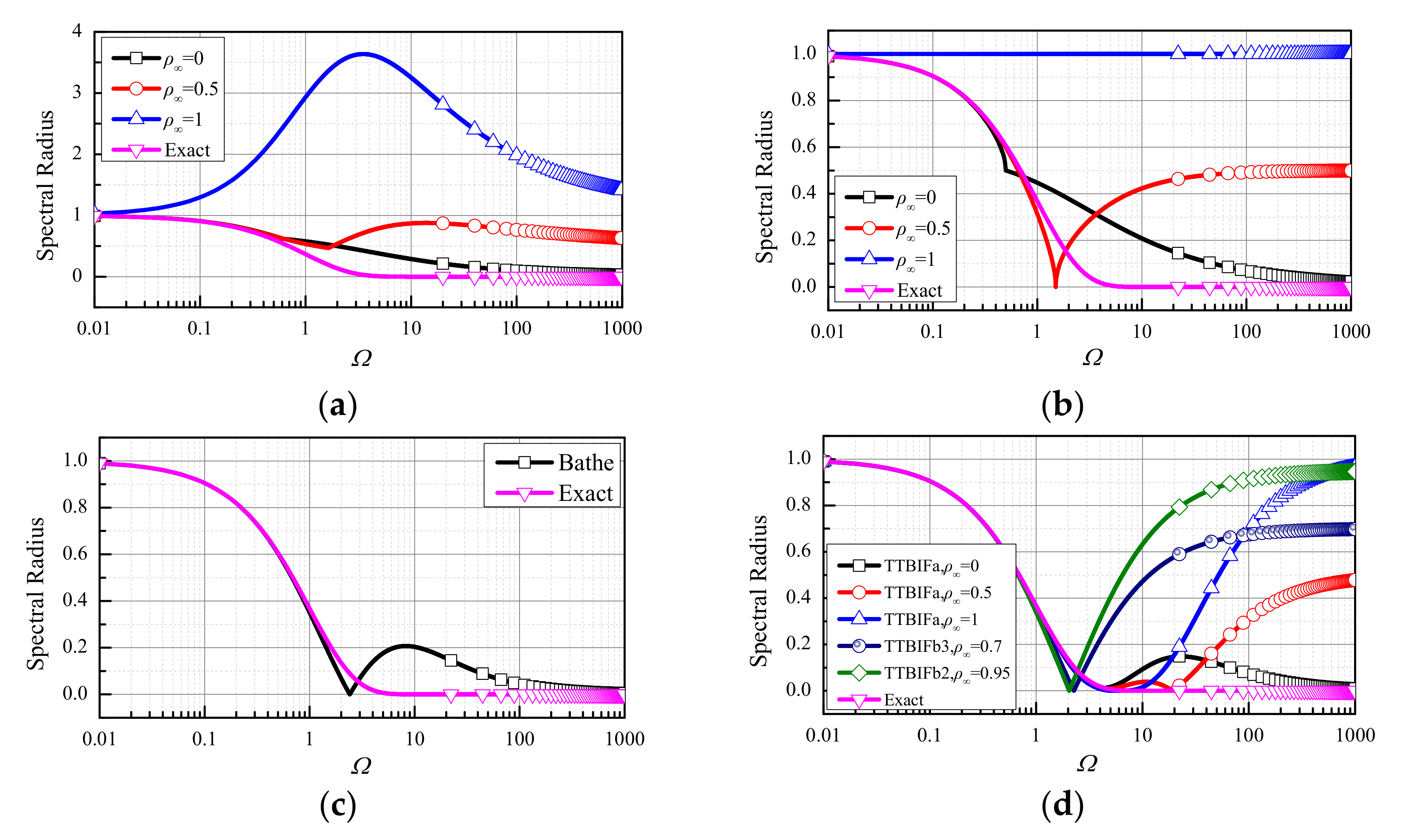
To compare the spectral characteristics of different methods in the presence of damping ratio, the numerical spectral radius and the exact spectral radius ρexact = exp(−ξΩ) [46] are shown in Figure 6. It can be concluded that:
- (1)
- if ξ ≠ 0, the generalized-α method may be unstable, as ρ(Ω) > 1;
- (2)
- if ρ∞ = 1, the physical damping has no effect on the ρ of the SS2 method, and if 0 ≤ ρ∞ < 1, the ρ of the SS2 method agrees well with the exact one in the range of 0 < Ω ≤ 0.3;
- (3)
- the ρ of the Bathe method matches well with the exact one in the range of 0 < Ω ≤ 1;
- (4)
- in the range of 0 < Ω ≤ 4, the ρ of the TTBIFa agrees well with the exact one, and the ρ of the TTBIFb is consistent with the exact one in the range of 0 < Ω ≤1.
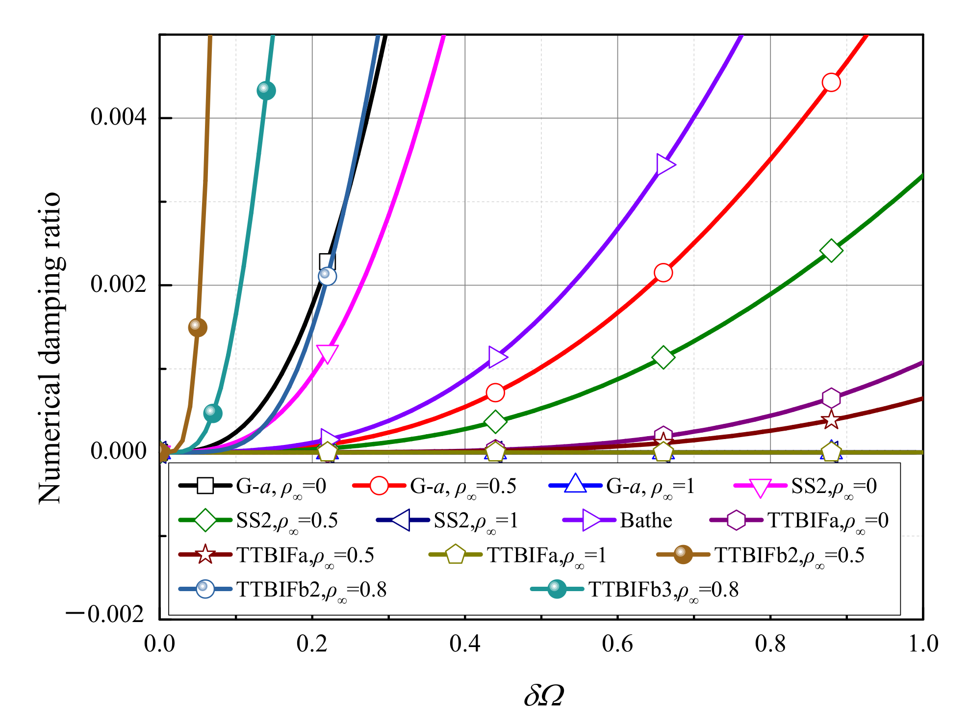
It can be found that for both undamped and damped systems, the TTBIFa’s spectral radius is more accurate than those of other methods. Then, the amplitude and phase accuracy are further compared, as shown in Figure 7 and Figure 8, in which one can see that:
- (1)
- the TTBIFa exhibits desirable amplitude and phase accuracy for δΩ ∈ (0, 1];
- (2)
- the TTBIFb2 has considerable amplitude and phase errors in the low-frequency range, but the third-order accurate TTBIFb3 has the highest phase accuracy in the range of δΩ ∈ (0, 0.1].
Hence, the use of TTBIFb2 is not recommended owing to its larger numerical errors, and the TTBIFb3 can be applied to damped systems considering that it can quickly damp out the unwanted information and it has higher phase accuracy. Similar phenomena can be observed for other TTBIFb2 and TTBIFb3 under different ρ∞; thus, they are not plotted herein for brevity.
4.2. Overshoot Characteristics
The overshooting phenomenon may occur in the first several time steps. For a convergent method, there is no overshoot as Ω → 0, so only the case of Ω → ∞ needs to be considered. The analysis of overshooting should take into account the effect of physical damping. With physical damping, first-order overshooting components enter into several well-known time integration methods [47] which were previously thought to exhibit zero-order overshooting. Therefore, this section discusses the overshoot characteristics of the TTBIF for undamped (ξ = 0) and damped (ξ = 1) cases. If Ω → ∞, the recursive schemes of the TTBIF at the first step (t = 0) can be derived from Equation (28); i.e.,
The above equations disclose that when Ω → ∞ with a large ∆t, displacement, velocity, and acceleration of the TTBIF in the first step decay to constants for arbitrary conditions. It can be seen in Equations (33)–(35) that the overshoot characteristics of the TTBIF are independent of the value of γ1, so this section discusses the TTBIFa only; refer to Figure 9, Figure 10, Figure 11 and Figure 12. The test equation (Equation (27)), two initial conditions are considered, including two situations, q(0) = 0, (0) = 1 and q(0) = 1, (0) = 0. One can see in Figure 9, Figure 10, Figure 11 and Figure 12 that the TTBIF does not have the overshoots for these two initial conditions, and the physical damping has no influence on the overshoot characteristics of the TTBIF.
4.3. Convergence Rates
The decrease rate of the absolute error as the step size decreases at a certain moment is defined as the convergence rate, which is usually employed to evaluate the accuracy order of a time integration method by displacement, velocity, and acceleration. In the test equation (Equation (27)), we assume that ξ = 2, ω = , and f(t) = sin2t; and the exact solution is x(t) = exp(−2t)(cost + 2sint) (8cos2t sin2t)/65. The absolute errors of the TTBIF at time t = 1 are shown in Figure 13, in which one can see that:
- (1)
- the TTBIFa method is strictly second-order accurate for displacement, velocity, and acceleration, and its computational accuracy can be improved with an increase in ρ∞;
- (2)
- the TTBIFb3 method can be third-order accurate for displacement, velocity, and acceleration;
- (3)
- the generalized-α method (G-α) is first-order accurate for acceleration when ρ∞ < 1.
The theoretical analysis given in this section illustrates that:
- (1)
- the low-frequency responses of the TTBIFa are more accurate, and it has the ability to damp out high-frequency modes; therefore, the TTBIFa are applicable to conservative systems and stiff systems;
- (2)
- the low-frequency response accuracy of the TTBIFb2 is low, so the TTBIFb2 is not practical;
- (3)
- the TTBIFb3 has strong numerical dissipation and lower numerical dispersion; hence, the TTBIFb3 is more suitable for damped systems.
Here, we provide a summary of the above time integration methods, and their accuracy, type of numerical dissipation, low-frequency accuracy, and scope of application are provided in Table 3, in which one can find that:
- (1)
- (2)
- among these methods, only TTBIF can achieve third-order accuracy for displacement, velocity, and acceleration, and it has numerical dissipation;
- (3)
- (4)
- from the values of and PE, one can see that among the second-order accurate methods, the TTBIFa’s low-frequency accuracy, including amplitude and phase, is the highest, meaning that it can give more accurate predictions when applied to dynamic problems, including structural dynamics and the multibody systems.
5. Numerical Experiments
To validate the desirable performances of the TTBIF, several benchmark multibody dynamic experiments are presented in this section. The generalized-α method [12], the SS2 method [26], and the Bathe method [31], are also considered. To ensure that the accuracy comparison was conducted with the same computational cost, the time step size relations of these methods were ∆t(Generalized-α method) = ∆t(SS2) = ∆t(Bathe)/2 = ∆t(TTBIF)/3. Therefore, in all examples, only the size of the generalized-α method is provided, and the reference solutions were obtained by the generalized-α method using a small time step size.
5.1. Flexible Beam
To show the advantages of the TTBIFa in stability, energy-conservation, and accuracy, this example considers a flexible beam model [48], as shown in Figure 14. The model parameters are: the length l = 3 m, the radius r = 0.02 m, the modulus of elasticity E = 2 × 10⁶ Pa, and the density ρ = 7200 kg/m3. In the original configuration, the beam is horizontal and has zero initial velocity. The beam is discretized by 20 elements. For damping out numerical oscillations induced by the spatial discretization, the ρ∞ = 0 is used in all methods.
The cantilever beam under the effect of gravity is considered first, in which the time step size of the generalized-α method is 0.001 s. In this case, the beam is assumed to fall under the effect of gravity, as g = 9.81 m/s2. The configurations of the cantilever beam at different moments are plotted in Figure 15, and the results are provided by the TTBIFa. One can see that this model represents an extreme case of a large deformation problem that involves high inertia forces. The free falling beam is a conservative system, and its mechanical energy (or total energy), consisting of the kinetic energy, the strain energy, and the potential energy, should be zero. Figure 16 shows the variations of the energy with time. It can be seen that (1) the generalized-α method loses stability, and the other methods can give convergent results; (2) among the convergent methods, with the increase in time, the total energies of the SS2 method and the Bathe method show considerable attenuation, whereas the TTBIFa preserves energy well.
Then, the simply supported beam is considered to compare the accuracies of these methods, and the size of the generalized-α method is also 0.001 s. In the second case, the flexible beam is accelerated by increasing the gravity constant to g = 30 m/s2. The numerical results and the absolute errors at mid-point of the beam are plotted in Figure 17, Figure 18 and Figure 19. It can be clearly seen that the TTBIFa’s accuracy is the highest.
Last, the accuracies of these methods in solving the problem of a flexible beam under the effect of vertical concentrated force f = 100 N, as shown in Figure 14c, are investigated, in which the size of the generalized-α method is assumed to be 0.001 s. The displacements of these methods for the case (x = l) and the case (x = l/2) are shown in Figure 20 and Figure 21, respectively. It can be seen that the TTBIFa has a considerable advantage in the aspect of accuracy.
5.2. Slider–Pendulum
As shown in Figure 22, the second example considers a slider–pendulum model [49] to demonstrate the accuracy and dissipation of the TTBIFa in dealing with rigid multibody systems. The slider is constrained by the spring, and one end of the pendulum is hinged to the center of mass of the slider. The system parameters are m1 = m2 = 1 kg, L = 1 m, J2 = 1/12 kg·m2, g = 9.81 m/s2, k = 1 N/m, and 1016 N/m for the compliant and stiff systems. ρ∞ = 0 is used in all methods, and the time step size of the generalized-α method is 0.06 s.
The compliant case (k = 1 N/m) is considered first, in which the slider is motivated by the horizontal velocity v0 = 1 m/s. Figure 23, Figure 24 and Figure 25 show that the TTBIFa performs best in the simulations. The results of the two single-step methods, the generalized-α method and the SS2 method, become more inaccurate with time. Additionally, the performances of these methods in dealing with numerical drifts are also considered here. The position constraint equation of this model has the form
The variations of Φ1 and Φ2 vs. time are plotted in Figure 26. It can be observed that the TTBIFa behaves best in eliminating the drift phenomenon.
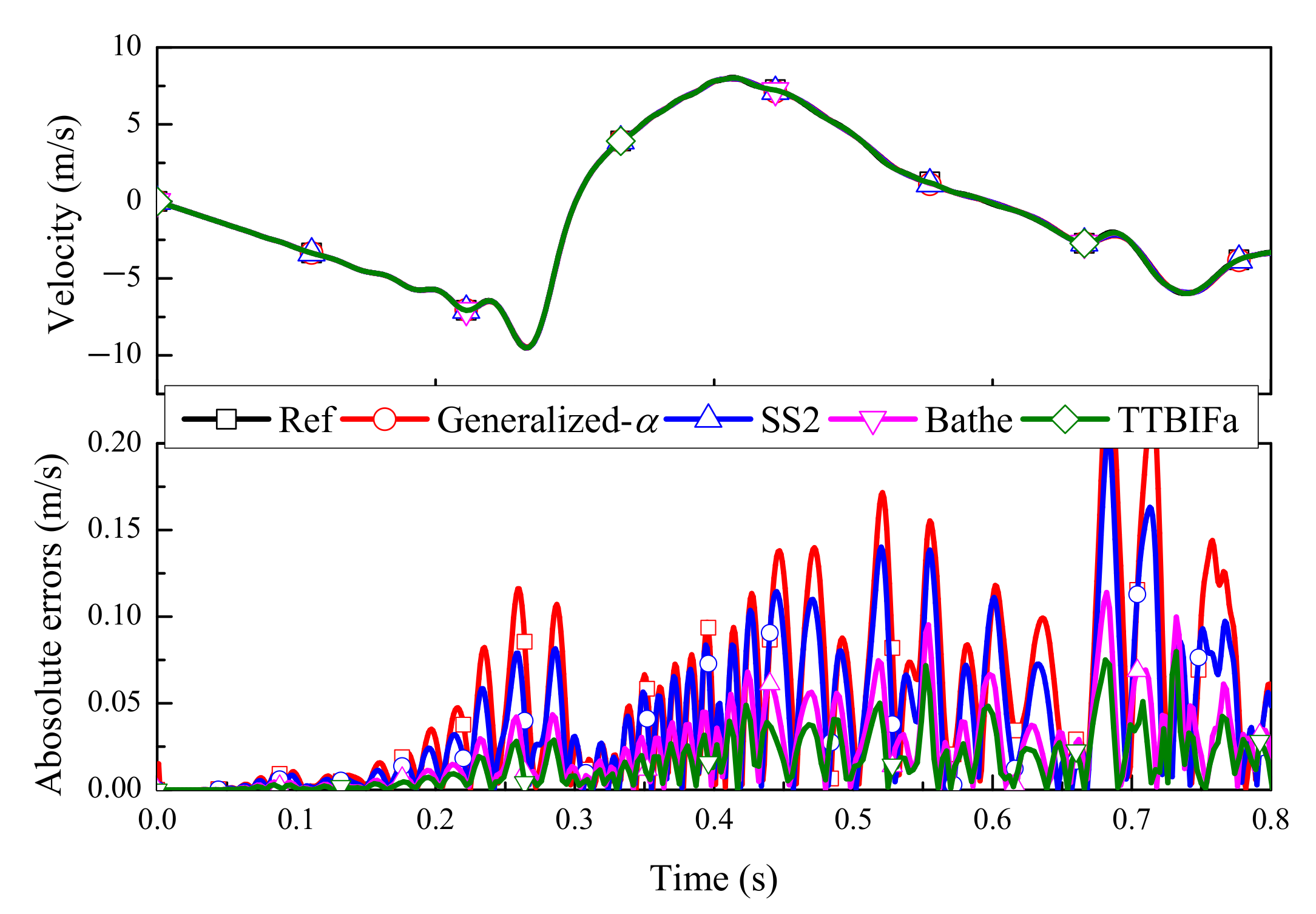
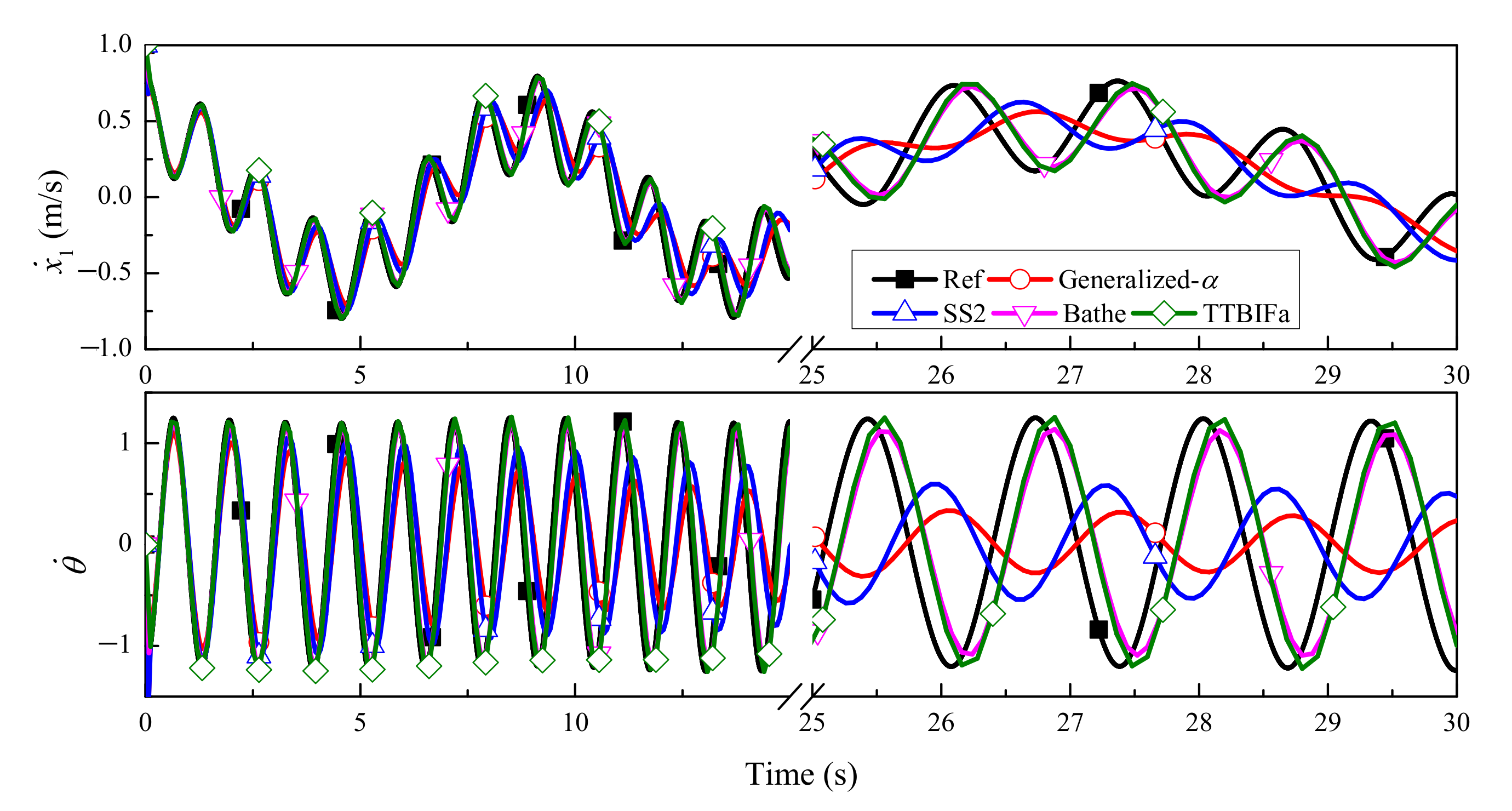
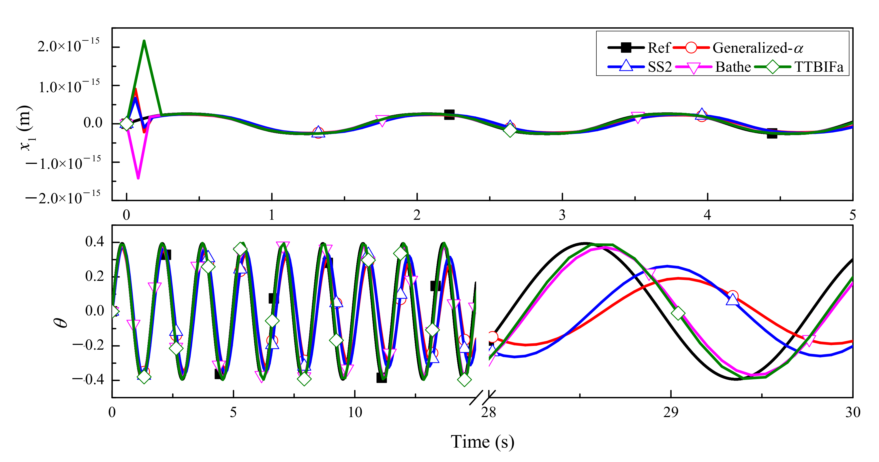
Then, the stiff case (k = 1016 N/m) is considered, in which the pendulum is motivated by the horizontal velocity v0 = 1 m/s. The time histories of x1 and θ are shown in Figure 27, from which one can see that all methods can effectively filter out the high-frequency information induced by the stiff constraint. Additionally, among these methods, the calculation accuracy of the TTBIFa is the highest.
5.3. Moving Cable
The last example considers a moving cable model, as shown in Figure 28, to test the performances of the TTBIFa and the TTBIFb3 in solving damped problems. The cable with spatial moving and axial material flow is part of the arresting-cable system [50]. The absolute nodal coordinate formulation (ANCF) in the framework of the arbitrary Lagrange–Euler (ALE) description is adopted to deal with the geometric nonlinearity and variable length of the moving cable elements. The model has two flexible ALE cable elements, and 12 degrees of freedom. Partial spatial movements or material flows of these nodes are given and realized by the kinematic time-varying constraint Φ, as follows:
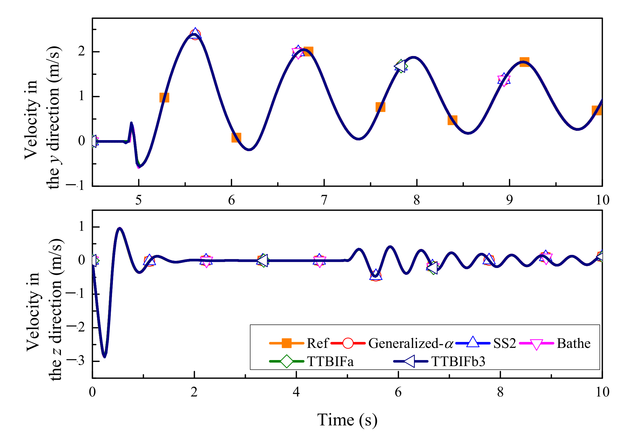
The ρ∞ = 0 is used in the generalized-α method, the SS2 method, and the TTBIFa to quickly filter out the numerical oscillations introduced by time-varying Φ. In addition, the third-order accurate TTBIFb3 with ρ∞ = 0.7 and γ1 = 1.64 is also considered here. In this example, the time step size of the generalized-α method is set to 0.01 s. The kinematic characteristics of mid-node 2 in the horizontal and vertical directions are shown in Figure 29, Figure 30 and Figure 31, in which one can see that the TTBIFb3 is the most accurate, followed by the TTBIFa. In addition, it can be found from Figure 31 that the acceleration calculated by the generalized-α method has larger errors compared with other methods.
6. Conclusions
The authors constructed a three-sub-step composite time integration method with controllable numerical dissipation in 2020, which was named as TTBIF [39]. This work presented a deep understanding of the TTBIF, and the algorithmic parameters of the TTBIF was further optimized, so two new optimized schemes of the TTBIF were developed and applied to the simulations of multibody systems.
The main contributions of this study can be summarized as follows:
- (1)
- The algorithmic parameter of the TTBIF (γ1) was optimized in this work to minimize local truncation error, yielding two new optimized schemes, the TTBIFa and the TTBIFbn (n = 2,3). The second-order accurate TTBIFa can accurately keep low-frequency information, and all sub-steps share the same effective stiffness matrix. The TTBIFb3 is third-order accurate, and possesses lower period errors than the second-order methods. Since the TTBIFb3 also has high dissipation capability, the TTBIFb3 is more suitable for damped systems.
- (2)
- The effects of algorithmic parameters on stability, dissipation, dispersion, overshoot, and convergence rate for damped and undamped systems were obtained in this work. The investigation is an important theoretical supplement for the TTBIF [39].
- (3)
- (4)
- The numerical experiments demonstrated that the second-order accurate, controllably dissipative, unconditionally stable TTBIFa exhibits advantages in accuracy, dissipation, stability, and energy-conservation, so it seems to be a good candidate for the response analysis of multibody systems.
Author Contributions
Conceptualization, Y.J.; Data curation, Y.J.; Funding acquisition, H.Z. and Y.X.; Software, Y.J. and H.Z.; Supervision, H.Z. and Y.X.; Validation, Y.J.; Writing—original draft, Y.J.; Writing—review & editing, H.Z. and Y.X. All authors have read and agreed to the published version of the manuscript.
Funding
This work was supported by the National Natural Science Foundation of China (12172023, 11872090), China Postdoctoral Science Foundation (2021M690391, 2022M710386), and the Outstanding Research Project of Shen Yuan Honors College BUAA (230121104).
Conflicts of Interest
The authors declare that they have no conflict of interest.
Appendix A. Derivations of the Recursion Equation
From the first relation given in Equation (17), the formulation of the first-sub-step can be rewritten as
Substituting the above expression (A1) into the equilibrium Equation (18) at t and t + γ1Δt can lead to
In terms of the second relation shown in Equation (17), the difference relations in the second sub-step can be reformulated as
Together with Equation (A2) and the equilibrium equation (Equation (18)) at t, t + γ1Δt and t + t + γ2Δt, we can get that
The last relation provided in Equation (17) can be rewritten as
Applying Equation (A2), Equation (A4), and the equilibrium equation (Equation (18)) at t, t + γ1Δt, t + γ2Δt, and t + Δt to Equation (A5) can yield the following recursion equation.
where A represents the TTBIF’s amplification factor.
Appendix B. Effective Stiffness Matrices and Load Vectors of the TTBIF
Consider the following linear ODEs:
where M, C, and K are the constant matrices; R is the external load vector. Applying the updating equations given in Equations (5)–(7) to Equation (A1) can yield the following time-stepping equations:
where the effective stiffness matrices are
and the effective load vectors have the forms
Appendix C. The Elements of the Amplification Matrix of the TTBIF
References
- Shabana, A.A. Dynamics of Multibody Systems; Cambridge University Press: New York, NY, USA, 2005. [Google Scholar]
- Ren, H.; Zhou, P. Implementation details of DAE integrators for multibody system dynamics. J. Dyn. Control 2021, 19, 1–28. (In Chinese) [Google Scholar]
- Wei, Y.; Deng, Z.; Li, Q.; Wang, B. Projected Runge-Kutta methods for constrained Hamiltonian systems. Appl. Math. Mech. Engl. Ed. 2016, 37, 1077–1094. [Google Scholar] [CrossRef]
- Marques, F.; Souto, A.; Flores, P. On the constraints violation in forward dynamics of multibody systems. Multibody Syst. Dyn. 2017, 39, 385–419. [Google Scholar] [CrossRef] [Green Version]
- Lin, S.; Chen, M. A PID type constraint stabilization method for numerical integration of multibody systems. J. Comput. Nonlinear Dyn. 2011, 6, 044501. [Google Scholar] [CrossRef]
- Vaiana, N.; Sessa, S.; Marmo, F.; Rosati, L. Nonlinear dynamic analysis of hysteretic mechanical systems by combining a novel rate-independent model and an explicit time integration method. Nonlinear Dyn. 2019, 98, 2879–2901. [Google Scholar] [CrossRef]
- Chang, S.Y. An unusual amplitude growth property and its remedy for structure- dependent integration methods. Comput. Methods Appl. Mech. Eng. 2018, 330, 498–521. [Google Scholar] [CrossRef]
- Hughes, T.J.R. The Finite Element Method: Linear Static and Dynamic Finite Element Analysis; Prentice-Hall: Englewood Cliffs, EC, USA, 1987. [Google Scholar]
- Chung, J.; Lee, J.M. A new family of explicit time integration methods for linear and nonlinear structural dynamics. Int. J. Numer. Methods Eng. 1994, 37, 3961–3976. [Google Scholar] [CrossRef]
- Kovacs, E.; Nagy, A.; Saleh, M. A new stable, explicit, third-order method for diffusion-type problems. Adv. Theory Simul. 2022, 5, 2100600. [Google Scholar] [CrossRef]
- Dong, S. BDF-like methods for nonlinear dynamic analysis. J. Comput. Phys. 2010, 229, 3019–3045. [Google Scholar] [CrossRef]
- Chung, J.; Hulbert, G.M. A time integration algorithm for structural dynamics with improved numerical dissipation: The generalized –α method. J. Appl. Mech. Trans. ASME 1993, 60, 371–375. [Google Scholar] [CrossRef]
- Wang, X.Y.; Wang, H.F.; Zhao, J.C.; Xu, C.Y.; Luo, Z.; Han, Q.K. Rigid-flexible coupling dynamics modeling of spatial crank-slider mechanism based on absolute node coordinate formulation. Mathematics 2022, 10, 881. [Google Scholar] [CrossRef]
- Hilber, H.M.; Hughes, T.J.R.; Taylor, R.L. Algorithms in structural dynamics. Earthq. Eng. Struct. Dyn. 1977, 5, 283–292. [Google Scholar] [CrossRef] [Green Version]
- Noh, G.; Bathe, K.J. For direct time integrations: A comparison of the Newmark and ρ∞-Bathe schemes. Comput. Struct. 2019, 225, 106079. [Google Scholar] [CrossRef]
- Arnold, M.; Hante, S. Implementation details of a generalized –α differential-algebraic equation Lie group method. J. Comput. Nonlinear Dyn. 2017, 12, 021002. [Google Scholar] [CrossRef]
- Wang, J.; Li, Z. Implementation of HHT algorithm for numerical integration of multibody dynamics with holonomic constraints. Nonlinear Dyn. 2015, 80, 817–825. [Google Scholar] [CrossRef]
- Bruls, O.; Cardona, A.; Arnold, M. Lie group generalized–α time integration of constrained flexible multibody systems. Mech. Mach. Theory 2012, 48, 121–137. [Google Scholar] [CrossRef]
- Wang, K.; Tian, Q.; Hu, H.Y. Non-smooth spatial frictional contact dynamics of multibody systems. Multibody Syst. Dyn. 2021, 53, 1–27. [Google Scholar] [CrossRef]
- Sherif, K.; Nachbagauer, K.; Steiner, W.; Laub, T. A modified HHT method for the numerical simulation of rigid body rotations with Euler parameters. Multibody Syst. Dyn. 2019, 46, 181–202. [Google Scholar] [CrossRef] [Green Version]
- Zhang, H.M.; Xing, Y.F. A three-parameter single-step time integration method for structural dynamic analysis. Acta Mech. Sin. 2019, 35, 112–128. [Google Scholar] [CrossRef]
- Wang, Y.Z.; Xue, T.; Tamma, K.K.; Maxam, D.; Qin, G. A three-time-level a posteriori error estimator for GS4-2 framework: Adaptive time stepping for second-order transient systems. Comput. Methods Appl. Mech. Eng. 2021, 384, 113920. [Google Scholar] [CrossRef]
- Lavrencic, M.; Brank, B. Comparison of numerically dissipative schemes for structural dynamics: Generalized- alpha vs. energy-decaying methods. Thin-Walled Struct. 2020, 157, 107075. [Google Scholar] [CrossRef]
- Zhang, H.M.; Xing, Y.F.; Ji, Y. An energy-conserving and decaying time integration method for general nonlinear dynamics. Int. J. Numer. Methods Eng. 2020, 121, 925–944. [Google Scholar] [CrossRef]
- Wu, B.; Pan, T.L.; Yang, H.W.; Xie, J.Z.; Spencer, B.F. Energy-consistent integration method and its application to hybrid testing. Earthq. Eng. Struct. Dyn. 2020, 49, 415–433. [Google Scholar] [CrossRef]
- Zhang, H.M.; Zhang, R.S.; Masarati, P. Improved second-order unconditionally stable schemes of linear multi-step and equivalent single-step integration methods. Comput. Mech. 2021, 67, 289–313. [Google Scholar] [CrossRef]
- Zhang, J. A-stable linear two-step time integration methods with consistent starting and their equivalent single-step and their equivalent single-step methods in structural dynamics analysis. Int. J. Numer. Methods Eng. 2021, 122, 2312–2359. [Google Scholar] [CrossRef]
- Zhang, H.M.; Zhang, R.S.; Zanoni, A.; Masarati, P. Performance of implicit A-stable time integration methods for multibody system dynamics. Multibody Syst. Dyn. 2022, 54, 263–301. [Google Scholar] [CrossRef]
- Ji, Y.; Xing, Y.F. A two-step time integration method with desirable stability for nonlinear structural dynamics. Eur. J. Mech. A Solids 2022, 94, 104582. [Google Scholar] [CrossRef]
- Bank, R.E.; Coughran, W.M.; Fichtner, W.; Gross, E.H.; Kent, S.R.; Rose, D.J. Transient simulation of silicon devices and circuits. IEEE Trans. Electron. Devices 1985, 32, 1992–2007. [Google Scholar] [CrossRef]
- Bathe, K.J.; Baig, M.M. On a composite implicit time integration procedure for nonlinear dynamics. Comput. Struct. 2005, 83, 2513–2524. [Google Scholar] [CrossRef]
- Chandra, Y.; Zhou, Y.; Stanciulescu, I.; Eason, T.; Spottswood, S. A robust composite time integration scheme for snap-through problems. Comput. Mech. 2015, 55, 1041–1056. [Google Scholar] [CrossRef] [Green Version]
- Wen, W.B.; Wei, K.; Lei, H.S.; Duan, S.Y.; Fang, D.N. A novel sub-step composite implicit time integration scheme for structural dynamics. Comput. Struct. 2017, 182, 176–186. [Google Scholar] [CrossRef]
- Xing, Y.F.; Ji, Y.; Zhang, H.M. On the construction of a type of composite time integration methods. Comput. Struct. 2019, 221, 157–178. [Google Scholar] [CrossRef]
- Li, J.Z.; Yu, K.P. A simple truly self-starting and L-stable integration algorithm for structural dynamics. Int. J. Appl. Mech. 2020, 12, 2050119. [Google Scholar] [CrossRef]
- Malakiyeh, M.M.; Shojaee, S.; Bathe, K.J. The Bathe time integration method revisited for prescribing desired numerical dissipation. Comput. Struct. 2019, 212, 289–298. [Google Scholar] [CrossRef]
- Noh, G.; Bathe, J. The Bathe time integration method with controllable spectral radius: The ρ∞-Bathe method. Comput. Struct. 2019, 212, 299–310. [Google Scholar] [CrossRef]
- Kim, W.; Choi, S.Y. An improved implicit time integration algorithm: The generalized composite time integration algorithm. Comput. Struct. 2018, 196, 341–354. [Google Scholar] [CrossRef]
- Ji, Y.; Xing, Y.F. An optimized three-sub-step composite time integration method with controllable numerical dissipation. Comput. Struct. 2020, 231, 106210. [Google Scholar] [CrossRef]
- Li, J.Z.; Zhao, R.; Yu, K.P. Directly self-starting higher-order implicit integration algorithms with flexible dissipation control for structural dynamics. Comput. Methods Appl. Mech. Eng. 2022, 389, 114274. [Google Scholar] [CrossRef]
- Liu, T.H.; Huang, F.L.; Wen, W.B.; He, X.H.; Duan, S.Y.; Fang, D.N. Further insights of a composite implicit time integration scheme and its performances on linear seismic response analysis. Eng. Struct. 2021, 241, 112490. [Google Scholar] [CrossRef]
- Zhang, J.Y.; Lei, S.; Liu, T.H.; Zhou, D.; Wen, W.B. Performance of a three-sub-step time integration method on structural nonlinear seismic analysis. Math. Probl. Eng. 2021, 2021, 1–20. [Google Scholar]
- Vaiana, N.; Sessa, S.; Marmo, F.; Rosati, L. A class of uniaxial phenomenological models for simulating hysteretic phenomena in rate-independent mechanical systems and materials. Nonlinear Dyn. 2018, 93, 1647–1669. [Google Scholar] [CrossRef]
- Vaiana, N.; Sessa, S.; Rosati, L. A generalized class of uniaxial rate-independent models for simulating asymmetric mechanical hysteresis phenomena. Mech. Syst. Signal Processing 2021, 146, 106984. [Google Scholar] [CrossRef]
- Wen, Y.K. Method for random vibration of hysteretic systems. ASCE- J. Eng. Mech. Div. 1976, 102, 249–263. [Google Scholar] [CrossRef]
- Zhang, J.; Liu, Y.H.; Liu, D.H. Accuracy of a composite implicit time integration scheme for structural dynamics. Int. J. Numer. Methods Eng. 2017, 109, 368–406. [Google Scholar] [CrossRef]
- Maxam, D.J.; Tamma, K.K. A re-evaluation of overshooting in time integration schemes: The neglected effect of physical damping in the starting procedure. Int. J. Numer. Methods Eng. 2022, 123, 2683–2704. [Google Scholar] [CrossRef]
- Berzeri, M.; Shabana, A.A. Development on simple models for the elastic forces in the absolute nodal co-ordinate formulation. J. Sound Vib. 2000, 235, 539–565. [Google Scholar] [CrossRef]
- Zhang, H.M.; Zhang, R.S.; Xing, Y.F.; Masarati, P. On the optimization of n-sub-step composite time integration methods. Nonlinear Dyn. 2020, 102, 1939–1962. [Google Scholar] [CrossRef]
- Zhang, H.; Guo, J.Q.; Liu, J.P.; Ren, G.X. An efficient multibody dynamic model of arresting cable systems based on ALE formulation. Mech. Mach. Theory 2020, 151, 103892. [Google Scholar] [CrossRef]
- Ji, Y.; Xing, Y.F.; Wiercigroch, M. An unconditionally stable time integration method with controllable dissipation for second-order nonlinear dynamics. Nonlinear Dyn. 2021, 53, 1951–1960. [Google Scholar] [CrossRef]
Figure 1.
Change of (A(1)(0) 1) with γ1. (a) 0 < γ1 < (2 − )/(1 + ρ∞), (b) γ1 > (2 + )/(1 + ρ∞) (ρ∞ ∈ [0, 0.6]), (c) γ1 > (2 + )/(1 + ρ∞) (ρ∞ ∈ [0.7, 0.95]).
Figure 1.
Change of (A(1)(0) 1) with γ1. (a) 0 < γ1 < (2 − )/(1 + ρ∞), (b) γ1 > (2 + )/(1 + ρ∞) (ρ∞ ∈ [0, 0.6]), (c) γ1 > (2 + )/(1 + ρ∞) (ρ∞ ∈ [0.7, 0.95]).


Figure 2.
Computational flowchart of the TTBIF for multibody systems governed by Equation (1).

Figure 3.
Spectral radius of the TTBIFa vs. Ω. (a) ρ∞ = 1, (b) ρ∞ = 0.8, (c) ρ∞ = 0.6, (d) ρ∞ = 0.4, (e) ρ∞ = 0.2, (f) ρ∞ = 0.
Figure 3.
Spectral radius of the TTBIFa vs. Ω. (a) ρ∞ = 1, (b) ρ∞ = 0.8, (c) ρ∞ = 0.6, (d) ρ∞ = 0.4, (e) ρ∞ = 0.2, (f) ρ∞ = 0.


Figure 4.
Spectral radius of the TTBIFbn vs. Ω. (a) ρ∞ = 0.9 (n = 2: black, solid; n = 3: red, dash), (b) ρ∞ = 0.8 (n = 2: black, solid; n = 3: red, dash), (c) ρ∞ = 0.7 (n = 2:black, solid; n = 3, γ1 = 1.64: red, dash; n = 3, γ1 = 3.47: blue, dash), (d) ρ∞ = 0.6, (e) ρ∞ = 0.4, (f) ρ∞ = 0.
Figure 4.
Spectral radius of the TTBIFbn vs. Ω. (a) ρ∞ = 0.9 (n = 2: black, solid; n = 3: red, dash), (b) ρ∞ = 0.8 (n = 2: black, solid; n = 3: red, dash), (c) ρ∞ = 0.7 (n = 2:black, solid; n = 3, γ1 = 1.64: red, dash; n = 3, γ1 = 3.47: blue, dash), (d) ρ∞ = 0.6, (e) ρ∞ = 0.4, (f) ρ∞ = 0.

Figure 5.
Spectral radii of the generalized-α method (G-α), SS2 method, Bathe method, and TTBIF vs. δΩ (ξ = 0).
Figure 5.
Spectral radii of the generalized-α method (G-α), SS2 method, Bathe method, and TTBIF vs. δΩ (ξ = 0).

Figure 6.
Spectral radius of the generalized-α method, SS2 method, Bathe method, TTBIF vs. Ω (ξ = 1). (a) Generalized-α method, (b) SS2 method, (c) Bathe method, (d) TTBIF.
Figure 6.
Spectral radius of the generalized-α method, SS2 method, Bathe method, TTBIF vs. Ω (ξ = 1). (a) Generalized-α method, (b) SS2 method, (c) Bathe method, (d) TTBIF.

Figure 7.
Numerical damping ratios of the generalized-α method (G-α), SS2 method, Bathe method, and TTBIF vs. δΩ.
Figure 7.
Numerical damping ratios of the generalized-α method (G-α), SS2 method, Bathe method, and TTBIF vs. δΩ.

Figure 8.
Period elongation ratios of the generalized-α method (G-α), SS2 method, Bathe method, and TTBIF vs. δΩ.
Figure 8.
Period elongation ratios of the generalized-α method (G-α), SS2 method, Bathe method, and TTBIF vs. δΩ.

Figure 9.
Displacement, velocity, and acceleration of the TTBIFa vs. ∆t/T for the case of ξ = 0, q(0) = 1, and (0) = 0.
Figure 9.
Displacement, velocity, and acceleration of the TTBIFa vs. ∆t/T for the case of ξ = 0, q(0) = 1, and (0) = 0.

Figure 10.
Displacement, velocity, and acceleration of the TTBIFa vs. ∆t/T for the case of ξ = 1, q(0) = 1, and (0) = 0.
Figure 10.
Displacement, velocity, and acceleration of the TTBIFa vs. ∆t/T for the case of ξ = 1, q(0) = 1, and (0) = 0.

Figure 11.
Displacement, velocity, and acceleration of the TTBIFa vs. ∆t/T for the case of ξ = 0, q(0) = 0, and (0) = 1.
Figure 11.
Displacement, velocity, and acceleration of the TTBIFa vs. ∆t/T for the case of ξ = 0, q(0) = 0, and (0) = 1.

Figure 12.
Displacement, velocity, and acceleration of the TTBIFa vs. ∆t/T for the case of ξ = 1, q(0) = 0, and (0) = 1.
Figure 12.
Displacement, velocity, and acceleration of the TTBIFa vs. ∆t/T for the case of ξ = 1, q(0) = 0, and (0) = 1.

Figure 13.
Absolute errors in displacement, velocity, and acceleration vs. ∆t.

Figure 14.
Flexible beam model. (a) Cantilever beam under the effect of gravity, (b) simply supported beam under the effect of gravity, (c) cantilever beam under the effect of vertical concentrated force.
Figure 14.
Flexible beam model. (a) Cantilever beam under the effect of gravity, (b) simply supported beam under the effect of gravity, (c) cantilever beam under the effect of vertical concentrated force.

Figure 15.
Configurations of the cantilever beam under the effect of gravity at different times.

Figure 16.
Time history of energies for the cantilever beam under the effect of gravity. (a) Generalized-α, (b) SS2, (c) Bathe, (d) TTBIFa.
Figure 16.
Time history of energies for the cantilever beam under the effect of gravity. (a) Generalized-α, (b) SS2, (c) Bathe, (d) TTBIFa.

Figure 17.
Displacement and absolute errors at mid-point for the simply supported beam under the effect of gravity.
Figure 17.
Displacement and absolute errors at mid-point for the simply supported beam under the effect of gravity.

Figure 18.
Velocity and absolute errors at mid-point for the simply supported beam under the effect of gravity.
Figure 18.
Velocity and absolute errors at mid-point for the simply supported beam under the effect of gravity.

Figure 19.
Acceleration and absolute errors at mid-point for the simply supported beam under the effect of gravity.
Figure 19.
Acceleration and absolute errors at mid-point for the simply supported beam under the effect of gravity.

Figure 20.
Displacement and absolute errors for cantilever beam subjected to the concentrated force at the free end (x = l).
Figure 20.
Displacement and absolute errors for cantilever beam subjected to the concentrated force at the free end (x = l).

Figure 21.
Displacement and absolute errors for cantilever beam subjected to the concentrated force at mid-point (x = l/2).
Figure 21.
Displacement and absolute errors for cantilever beam subjected to the concentrated force at mid-point (x = l/2).

Figure 22.
Slider-pendulum model.

Figure 23.
Results of x1 and θ for the compliant case.

Figure 24.
Results of 1 and for the compliant case.

Figure 25.
Results of 1 and for the compliant case.

Figure 26.
Results of position constraint for the compliant case.

Figure 27.
Time histories of x1 and θ for the stiff case.

Figure 28.
Moving cable model (β is the stiffness proportional to the Rayleigh damping factor).

Figure 29.
Displacement of mid-node 2.

Figure 30.
Velocity of mid-node 2.

Figure 31.
Acceleration of mid-node 2.


Table 1.
Accuracy of the TTBIF for the case of 0 < γ1 < (2 −)/(1 + ρ∞).
| ρ∞ | γ1 | γ1 − 2θ3 | n (Accuracy Order) | φ(γ1, ρ∞) = 0 | A(3)(0) = 1 |
|---|---|---|---|---|---|
| 0 | 0.360850612858797128269166267064 | −3.3307 × 10⁻¹⁶ | 2 | Yes | No |
| 0.1 | 0.357238916409318421781603138200 | 2.7756 × 10⁻¹⁶ | 2 | Yes | No |
| 0.2 | 0.353891613236446119002830462643 | 3.8858 × 10⁻¹⁶ | 2 | Yes | No |
| 0.3 | 0.350771031685691357865125234250 | −5.5511 × 10⁻¹⁷ | 2 | Yes | No |
| 0.4 | 0.347847215754394957955227697970 | −1.1102 × 10⁻¹⁶ | 2 | Yes | No |
| 0.5 | 0.345095922844178112406277539906 | 0 | 2 | Yes | No |
| 0.6 | 0.342497237181383015615320747048 | 1.6653 × 10⁻¹⁶ | 2 | Yes | No |
| 0.7 | 0.340034583544953015899346977758 | 1.6653 × 10⁻¹⁶ | 2 | Yes | No |
| 0.8 | 0.337694009358335747749068721842 | 0 | 2 | Yes | No |
| 0.9 | 0.335463651513773966300486501975 | 2.2204 × 10⁻¹⁶ | 2 | Yes | No |
| 1 | 1/3 | 1.6653 × 10⁻¹⁶ | 2 | Yes | No |
Table 2.
Accuracy of the TTBIF for the case of γ1 > (2 + )/(1 + ρ∞).
| ρ∞ | γ1 | γ1 − 2θ3 | n (Accuracy Order) | φ (γ1, ρ∞) = 0 | A(3)(0) = 1 |
|---|---|---|---|---|---|
| 0 | 4.37120019471008016525828007444 | 1.7764 × 10⁻¹⁵ | 2 | Yes | No |
| 0.1 | 3.86720615297079833146530716573 | 0 | 2 | Yes | No |
| 0.2 | 3.44197544571550477178258216569 | −1.7764 × 10⁻¹⁵ | 2 | Yes | No |
| 0.3 | 3.07637810817689875070626896811 | 3.9968 × 10⁻¹⁵ | 2 | Yes | No |
| 0.4 | 2.75641330487022065008264507216 | 2.6645 × 10⁻¹⁵ | 2 | Yes | No |
| 0.5 | 2.47130235794770540209427935717 | −7.1054 × 10⁻¹⁵ | 2 | Yes | No |
| 0.6 | 2.21211453543800466240456025712 | −8.8818 × 10⁻¹⁶ | 2 | Yes | No |
| 0.7 | 1.64139639997267794413460251235 | 9.1071 | 3 | No | Yes |
| 3.47338081413162491628554562340 | 2.1307 | 3 | No | Yes | |
| 1.97043992476900261510531844803 | 2.6645 × 10⁻¹⁵ | 2 | Yes | No | |
| 0.8 | 5.85462097569634387639325723285 | 4.7010 | 3 | No | Yes |
| 1.73618888723806906658432806893 | −1.7097 × 10⁻¹⁴ | 2 | Yes | No | |
| 0.9 | 12.6079265663953545839603975764 | 11.5479 | 3 | No | Yes |
| 1.49018874467779463098199628280 | 3.7748 × 10⁻¹⁵ | 2 | Yes | No | |
| 0.95 | 25.9730301544759925036487402394 | 24.9458 | 3 | No | Yes |
| 1.34386843962051960588155452569 | 3.0198 × 10⁻¹⁴ | 2 | Yes | No |
Table 3.
Numerical characteristics of some advanced time integration methods.
| Method | Number of Sub-Step | Dissipation | Accuracy (ξ ≠ 0, f ≠ 0) | Low-Frequency (ξ = 0, δΩ = 1, ρ∞ = 0) | Scope of Application | ||||
|---|---|---|---|---|---|---|---|---|---|
| Dis. | Vel. | Acc. | PE | ODEs | DAEs | ||||
| Generalized-α [12] | 1 | A-stability | 2 | 2 | 1 | 0.06118 | 0.24744 | Yes | Yes |
| Bathe [31] | 2 | L-stability | 2 | 2 | 2 | 0.01214 | 0.10516 | Yes | Yes |
| ρ∞-Bathe [37] | 2 | A-stability | 2 | 2 | 2 | 0.01214 | 0.10516 | Yes | No |
| Kim [38] | 2 | A-stability | 2 | 2 | 2 | 0.01214 | 0.10516 | Yes | No |
| TTBDF [32] | 3 | L-stability | 2 | 2 | 2 | 0.00213 | 0.11003 | Yes | No |
| TTBIFa | 3 | A-stability | 2 | 2 | 2 | 0.00108 | 0.10479 | Yes | Yes |
| TTBIFb3 | 3 | 3 | 3 | / | / | ||||
Publisher’s Note: MDPI stays neutral with regard to jurisdictional claims in published maps and institutional affiliations. |
© 2022 by the authors. Licensee MDPI, Basel, Switzerland. This article is an open access article distributed under the terms and conditions of the Creative Commons Attribution (CC BY) license (https://creativecommons.org/licenses/by/4.0/).
Share and Cite
MDPI and ACS Style
Ji, Y.; Zhang, H.; Xing, Y. New Insights into a Three-Sub-Step Composite Method and Its Performance on Multibody Systems. Mathematics 2022, 10, 2375. https://0-doi-org.brum.beds.ac.uk/10.3390/math10142375
AMA Style
Ji Y, Zhang H, Xing Y. New Insights into a Three-Sub-Step Composite Method and Its Performance on Multibody Systems. Mathematics. 2022; 10(14):2375. https://0-doi-org.brum.beds.ac.uk/10.3390/math10142375
Chicago/Turabian StyleJi, Yi, Huan Zhang, and Yufeng Xing. 2022. "New Insights into a Three-Sub-Step Composite Method and Its Performance on Multibody Systems" Mathematics 10, no. 14: 2375. https://0-doi-org.brum.beds.ac.uk/10.3390/math10142375
Note that from the first issue of 2016, this journal uses article numbers instead of page numbers. See further details here.