A Two-Stage Model with an Improved Clustering Algorithm for a Distribution Center Location Problem under Uncertainty

Abstract

Distribution centers are quite important for logistics. In order to save costs, reduce energy consumption and deal with increasingly uncertain demand, it is necessary for distribution centers to select the location strategically. In this paper, a two-stage model based on an improved clustering algorithm and the center-of-gravity method is proposed to deal with the multi-facility location problem arising from a real-world case. First, a distance function used in clustering is redefined to include both the spatial indicator and the socio-economic indicator. Then, an improved clustering algorithm is used to determine the optimal number of distribution centers needed and the coverage of each center. Third, the center-of-gravity method is used to determine the final location of each center. Finally, the improved method is compared with the traditional clustering method by testing data from 12 cities in Inner Mongolia Autonomous Region in China. The comparison result proves the proposed method’s effectiveness.

1. Introduction

Selecting a proper site for a distribution center can effectively save costs, increase profits, improve customer satisfaction and reduce circulation time. Therefore, the location problem has been one of the most important decisions in logistics system planning [1]. Among these, the selection of distribution center sites has become one of the most popular research interests in logistics management. Readers interested in this field could refer to some recent research [2,3,4,5,6,7].

As the logistics in real-world become increasingly complicated due to factors that significantly increase the uncertainty in logistics planning, such as economy development, the prevalence of online retailing, increasing natural disasters, etc. It is necessary to introduce more indicators to deal with the uncertainty during the site selection process. This research includes demand uncertainty in the model described in a proper mathematical function, which takes both the spatial condition and the economic condition into consideration when selecting the proper locations for distribution centers. Hopefully, this research could provide a planning strategy for the selection of distribution center sites.

In this paper, all data is extracted from a real case of 12 cities in Inner Mongolia Autonomous Region, China. The author proposes a two-stage model based on an improved clustering algorithm and the center-of-gravity method to solve the location problem of distribution centers and provides a strategy for the logistics transportation in this case. The improved model proposed in this paper is compared with the traditional clustering method by testing data from 12 cities and is proved to be effective. The main work of this paper is as follows:

• Proposes a modified distance function takes both spatial indicators and socio-economic indicators into consideration, which makes the model match the real case better.
• Divides demand points into different regions using an improved clustering algorithm first, then uses the center-of-gravity method to modify the clustering center to select the location of the distribution center in each region.
• Compares the new model with the traditional clustering method using the data from a real case. The results indicate that the method proposed in this paper has a better performance.

The remainder of this paper is organized as follows. Section 2 reviews the literature on location problems. Section 3 presents the methodology of a two-stage model, including the improved clustering algorithm and the center-of-gravity method. Section 4 describes the obtained results using the proposed model. Section 5 compares the results between proposed model and different clustering algorithms. Section 6 concludes the research.

2. Literature Review

The location problem (LP) is a classical problem. The original problem can be traced back to the Fermat problem. The first industrial application of the Fermat problem was proposed by Alfred Weber in 1909 and called the Weber problem [8]. The purpose of the Weber problem is to find the location of a warehouse to minimize the total distance among all customers. Ever since Weber’s seminal work, LP has been booming in both the academical world and the industrial world. In previous researches, LP is well classified on the basis of model assumptions, constraints and objectives functions [9].

Based on the number of facilities involved, the location problem could also be classified into two categories, the single-facility location problem (SFLP) or the multi-facility location problem (MFLP). The SFLP is to determine the location of a single facility using the criteria of distance and cost. The common methods include the Weiszfeld method [10] and the center-of-gravity method [11]. However, one single facility might not be able to meet the increased service demand for its capacity is limited. This is where it becomes a multi-facility location problem, which is the problem to be studied in this paper.

The MFLP is commonly seen in humanitarian relief [12,13], emergency response [14], health care facility locations [15,16] and other fields. The objective function and criteria for facility location are considered from different perspectives in many studies, such as total cost, total transportation time and satisfaction [17]. Because MFLP covers a wide range and need to consider many factors, it can be divided into different problems, for example, it could be divided as the deterministic problem if the information in the problem is determined, and the probabilistic and stochastic problem if not. The former mainly focuses on coverage maximization [18,19] and resource minimization [20]. The latter had been largely discussed in earlier researches on the uncertainties of location problems, such as uncertain demand [21,22] and disruption risk [23]. Probabilistic and stochastic location problems can be divided into stochastic programming problems [24] and robust optimization problems [25]. For the detailed classification of MFLPs, interested readers can refer to Wang et al. [26].

There are two commonly methodologies used in MFLP researches: exact methods and heuristic algorithms [27]. In early researches, the scale of the location problem is usually small. Branch-and-bound [28] and cutting plane [29] are quite popular. However, with the expansion of the problem scales and the increase of the constraints, it becomes difficult to obtain the accurate solution. Finding a proper solution of a large-scale problem in a reasonable time has become the mainstream of LP researches, among which, the heuristic algorithm has been proposed for this purpose. Commonly used heuristic algorithms include genetic algorithm [30], particle swarm optimization [31], tabu search [32], cuckoo search [33] and Lagrangian relaxation [34]. However, the most distinctive disadvantage of heuristic algorithms is the computationally burdensome to find the best solution.

How to deal with the computational burden has then become many researchers’ interests. One widely adopted perspective is the clustering-based algorithms. By defining the location problem as a kind of clustering problem, the researcher would divide customers or demand points into different clusters, each of which is supplied by one facility. Then there would be only one SFLP in each cluster needs to be solved. Thus, by decomposing the multi-facility location problem (MFLP) into multiple single-facility location problems (SFLP), the researcher could simplify the complexity of calculation [35]. Among those researchers, Esnaf and Kucukdeniz [36] proposed a hybrid method using the fuzzy clustering algorithm to divide the whole region into certain number of areas, each supplied by one very facility, then they used the center-of-gravity method to select the location point of each facility. Kuecuekdeniz et al. [37] proposed a method which integrates fuzzy c-means and convex programming for solving a capacitated MFLP, where fuzzy c-means is used to convert an MFLP to an SFLP. Gupta et al. [38] used fuzzy c-means and particle swarm optimization to optimize the locations of public service centers. Researches mentioned above proved that the clustering-based algorithms are applicable in practice [39]. Nonetheless, few researchers have dedicated to improving the distance function in clustering.

In this paper, an MFLP of distribution centers arising from a real-world case is studied with clustering-based algorithms. The author uses the clustering algorithm to decompose the MFLP into multiple SFLPs and then uses the center-of-gravity method to select the locations of distribution centers by solving each SFLP. The work differs clearly from the previous literature. In this paper, both spatial and socio-economic indicators are well embedded in the clustering method. An improved distance function is proposed to explain the clustering results affected by the two types of indicators. Furthermore, the effectiveness of the proposed method is proved by a comparison on different methods.

3. Methodology

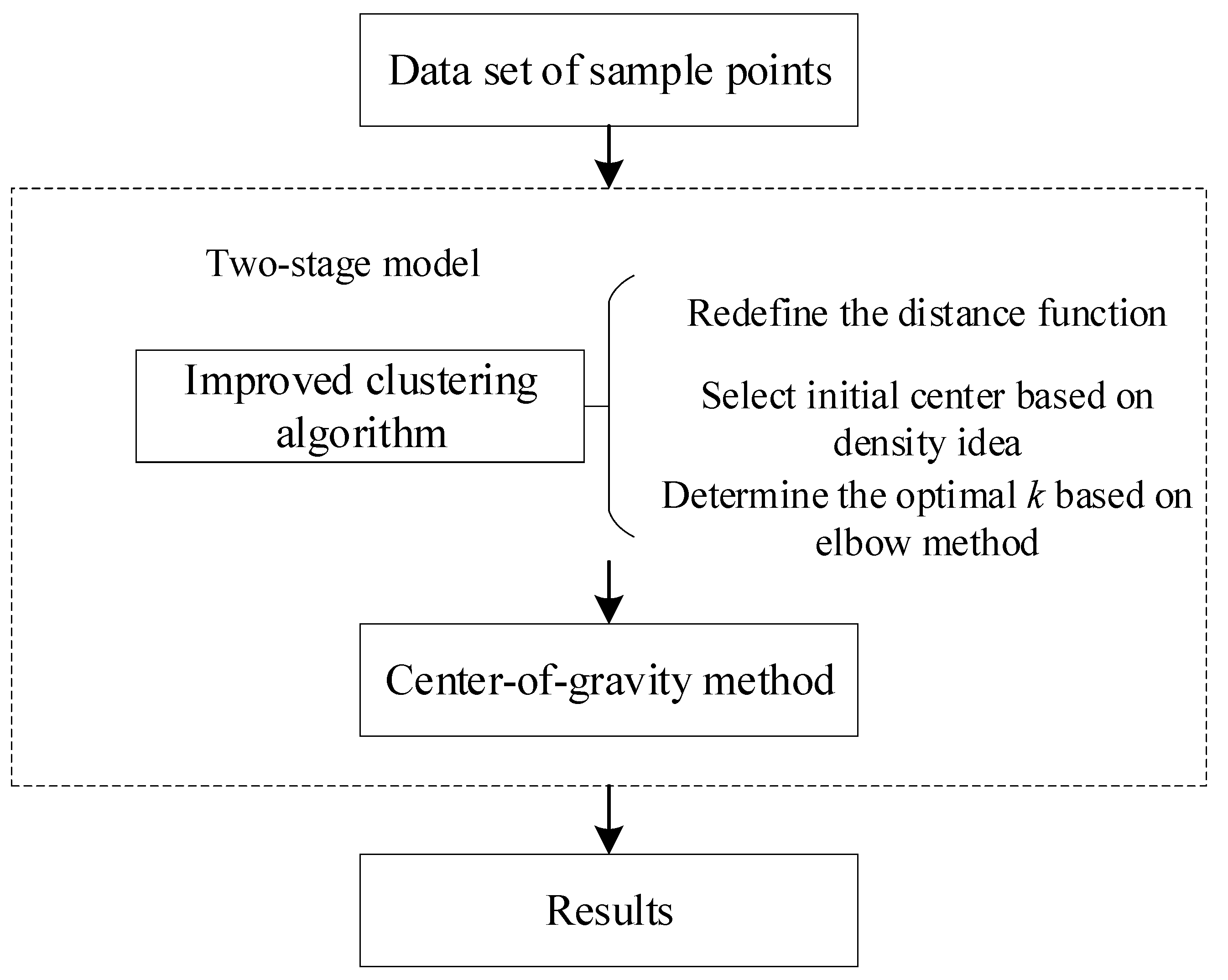
The proposed two-stage model (2SM) aims to compute the optimal number and locations of distribution centers with minimal total transportation cost. The structure of the model is composed of two sequential stages.

• Determine the optimal number of distribution centers by improved clustering for an MFLP.

In this stage, the author proposes an improved K-Medoids clustering algorithm to classify the demand points and determine the optimal clustering strategy. The improved clustering algorithm can be summarized as follows:

• Redefine the distance function by introducing three socio-economic indicators.
• Select the initial clustering center based on the density to improve the algorithm’s efficiency.
• Use the elbow method to determine the optimal number of clusters.

2.

Determine the optimal distribution center location by the center-of-gravity method for each SFLP.

After clustering, the location of each cluster distribution center is solved as a SFLP by employing the center-of-gravity method, which optimizes transportation cost. The framework of the model is given in Figure 1.

3.1. Improved Clustering Algorithm

The clustering algorithm [40] is a kind of unsupervised machine learning method. Its main idea is to divide the objects into different clusters to maximize the object similarity in each cluster and minimize the object similarity between any two clusters. To deal with noise data and outliers effectively, the author employs the K-Medoids clustering algorithm and modifies it to fit the work. The K-Medoids clustering algorithm [41,42] is an adjustment of the classical K-Means clustering algorithm. The pseudocodes for the K-Medoids are shown in Algorithm 1.

Algorithm 1K-Medoids Clustering Algorithm

Input: Data points ${\left\{x_i\right\}}_{i=1}^N$, number of clusters $K$ Choose different $x_i$ as initial clustering center $c_k$ for $k=1$ to $K$ Set $C_k\leftarrow \left\{c_k\right\}$ for $k=1$ to $K$ for $i=1$ to $K$ do $C_p\leftarrow C_p{\displaystyle \cup }\left\{x_i\right\}$, where $\mathrm{p}={\mathrm{argmin}}_{p\in I_1^K}d\left(x_i,c_P\right)$ end while allocation result of any $x_i$ changed do for $k=1$ to $K$                                $c_k\leftarrow {\mathrm{argmin}}_{x_i\in C_k}{\displaystyle \sum }_{x_t\in C_k}d\left(x_t,x_i\right)$ end for $i=1$ to $N$ do     if $x_i\in C_{k^{\prime }}$ and $d\left(x_i,c_k\right)<d\left(x_i,c_{k^{\prime }}\right)$ then     $C_k\leftarrow C_k{\displaystyle \cup }\left\{x_i\right\}$ and $C_{k^{\prime }}\leftarrow C_{k^{\prime }}\backslash \left\{x_i\right\}$     end end end Output: Clustering results ${\left\{C_k\right\}}_{k=1}^K$

Different from the K-Means, in the iterative process, the K-Medoids selects the data point closest to the data’s mean in the cluster as the new clustering center instead of choosing the average of all data points.

In the clustering algorithms, there are three factors affect the performance of clustering directly: distance measurement, algorithm efficiency and number of clusters. In consideration of the factors, an improved clustering method is proposed to meet the real-world situation.

3.1.1. Redefine the Distance Function

Euclidean distance is a common distance function in clustering algorithm that measures the distance between two points in m-dimensional space. The two-dimensional distance function considering the longitude and the latitude is as follows:

$$D_{ij}=\sqrt{{\left(x_i-x_j\right)}^2-{\left(y_i-y_j\right)}^2}$$

(1)

where $D_{ij}$ measures the distance between point $i$ and point $j$; $x_i$ and $x_j$ are the longitudes of point $i$ and point $j$, respectively; and $y_i$ and $y_j$ are the latitudes of point $i$ and point $j$, respectively.

Euclidean distance is simple and effective when dealing with homogeneous indicators. But when the indicators are different, it misses some practical interpretability. To cope with this setback, the author redefines the distance function considering both spatial indicators and socio-economic indicators. The spatial indicators represent the actual distance between two points. The socio-economic indicators reflect the logistics-level score of each point. The detailed computing process is as follows.

(1)

Compute the logistics-level score.

The logistics-level score proposed in this research mainly considers three dimensions: economy development, traffic congestion and total logistics demand, which is represented respectively by the per capita disposable income of urban residents, the population density and the permanent urban population, as shown in

Table 1. The indicator composition of the logistics-level score.

Dimension	Indicator
Economy development	per capita disposable income of urban residents
Traffic congestion	population density
Total logistics demand	permanent urban population

. Note that there is no available data on population density. Instead, the ratio of permanent urban residents to urban built-up area is used as in Equation (2).

$$population density=\frac{permanent urban population}{urban built up area}$$

(2)

As the actual data of the corresponding indicators is obtained, the author computes each city’s logistics-level score using the entropy weight method, which is used to determine the weight coefficient of each indicator by computing the information entropy. To a certain extent, the entropy weight method can avoid subjective judgment when determining weight coefficients [43]. The smaller the information entropy value of one indicator is, the larger the weight coefficient assigned to it becomes [44]. The logistics-level score is computed as Equations (3)–(8):

First, the data are normalized by Equations (3) and (4):

$$Y_{ij}=\frac{X_{ij}-\underset{i}{\min }\left(X_{ij}\right)}{\underset{i}{\max }\left(X_{ij}\right)-\underset{i}{\min }\left(X_{ij}\right)}$$

(3)

$$Y_{ij}=\frac{\underset{i}{\max }\left(X_{ij}\right)-X_{ij}}{\underset{i}{\max }\left(X_{ij}\right)-\underset{i}{\min }\left(X_{ij}\right)}$$

(4)

Equation (3) is the normalized formula of the utility indicator, and Equation (4) is the normalized formula of the cost indicator. $X_{ij}$ is the $j$th ($j=1,2\dots ,m$) indicator of city $i$ ($i=1,2\dots ,n$). $Y_{ij}$ is the indicator data after normalization. Since the greater the population density is, the greater the traffic congestion becomes, population density should be considered as the cost indicator. The other two indicators are utility indicators.

Then, the information entropy is computed by Equations (5) and (6):

$$P_{ij}=Y_{ij}/{\displaystyle \sum }_{i=1}^n{Y}_{ij}$$

(5)

$$E_j=-\frac{1}{\mathit{ln}n}{\displaystyle \sum }_{i=1}^n{P}_{ij}\mathit{ln}{P}_{ij}$$

(6)

where $P_{ij}$ is the weight of city $i$ in the $j$th indicator and $E_j$ is the information entropy of the $j$th indicator.

After that, the weights of the indicators are computed by Equation (7):

$$W_j=\left(1-E_j\right)/\left(n-{{\displaystyle \sum }}_{j=1}^m{E}_j\right)$$

(7)

where $W_j$ is weight of the $j$th indicator.

Finally, the logistics-level score of each city is computed by Equation (8):

$$Z_i={\displaystyle \sum }_{j=1}^m{Y}_{ij}{W}_j$$

(8)

where $Z_i$ is the logistics-level score of city $i$.

(2)

Define the distance between two points:

$$D\left(X_i,X_j\right)=\frac{D_{ij}^2}{{\left(Z_i{Z}_j\right)}^u}$$

(9)

In Equation (9), $D\left(X_i,X_j\right)$ measures the distance between any two cities, which is affected by two distance indicators: spatial and socio-economic. $D_{ij}^2$ is the spatial distance between any two cities, which represents the spatial indicators. The greater the spatial distance is, the greater the distance between the two cities becomes.$Z_i{Z}_j$ is the logistics score distance between any two cities, which represents the socio-economic indicators. $Z_i$ and $Z_j$ are the logistics-level scores of city $i$ and city $j$, respectively. The greater the logistics score distance is, the closer the connection between the two cities at the logistics level lies, and the smaller the distance between the two cities in the clustering process becomes. $u$ represents the degree of influence of the logistics-level score in the distance function between any two cities. The larger $u$ is, the greater the influence of the logistics-level score becomes. When $u$ is 0, the distance function is equivalent to the Euclidean distance.

3.1.2. Select the Initial Clustering Center

To reduce the time complexity of the clustering algorithm effectively and avoid the interference of noise data, the author introduces the idea of density into the clustering algorithm to determine the initial clustering center in this research. The steps of selecting the initial clustering center are as follows.

First, the domain radius $r_a$ of the demand points $X_i$ is computed by Equation (10):

$$r_a=\frac{1}{2}max\{\Vert X_i-X_k\Vert \}$$

(10)

The domain radius $r_a$ measures the maximum distance between $X_i$ and other demand points.

Then, the density factor $D_i$ of $X_i$ is computed by Equation (11):

$$D_i={\displaystyle \sum }_{j=1}^{n}exp\left[-\frac{\Vert X_i-X_j\Vert {}^2}{{\left(2r_a\right)}^2}\right]$$

(11)

A larger $D_i$ means that more demand points surround $X_i$, i.e., $X_i$ has a closer relationship with other points. The point with a greater density factor is more likely to be a clustering center. The exponential function could make sure that the point surrounded by more demand has a greater density factor.

After figuring out the density factors of all demand points, the factors are arranged in the descend order. Then, the demand points are selected corresponding to the top $k$ density factors as the initial clustering center.

3.1.3. Determine the Optimal k

The clustering algorithm aims to divide the similar sample points into the same cluster and effectively distinguish the dissimilar sample points. In this process, $k$ will significantly affect the final clustering performance. To obtain the optimal clustering results, it is necessary to determine the optimal selection of $k$ before clustering. In this research, the elbow method is used to obtain the optimal $k$ by computing the sum of the squares of error (SSE) between the sample points and their respective clustering centers. The equation for computing SSE is Equation (12):

$$SSE={\displaystyle \sum }_{i=1}^k{\displaystyle \sum }_{x\in C_i}{\left(x-P_i\right)}^2$$

(12)

where $C_i$ represents the $i$th cluster, $P_i$ is the clustering center of $C_i$ and $x$ is the point belonging to the $C_i$.

The core idea of the elbow method lies in the following: With the increase in cluster number $k$, sample division will be more refined, and the aggregation degree of each cluster will be gradually improved; thus, SSE will gradually become smaller. In addition, when $k$ is less than the optimal cluster number, SSE decreases greatly because the increase of $k$ will greatly increase the degree of aggregation of each cluster. However, when $k$ reaches the optimal cluster number, the return of aggregation degree obtained by increasing $k$ decreases rapidly. This means decrease of SSE will tend to be gentler as $k$ continues to increase.

3.1.4. The Flowchart of Clustering Algorithm

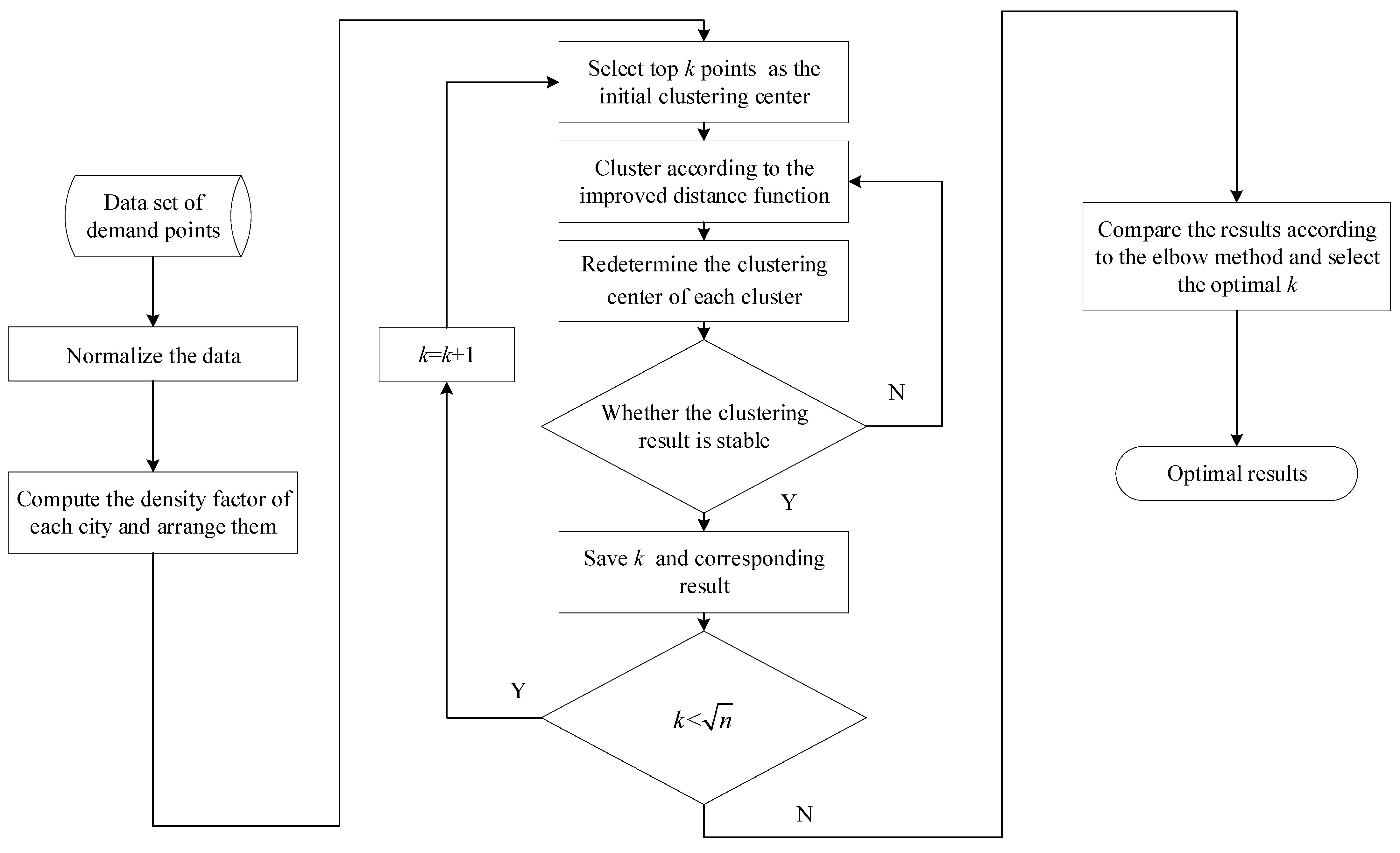
Based on the improvements discussed above, the clustering algorithm flow is as follows:

Step 1: Obtain the data of each city required by the model, normalize the data for each indicator to eliminate the dimensional influence.

Step 2: Compute the density factor of each city and arrange each city in the order of density factor from large to small.

Step 3: Take the top $k$ points in Step 2 as clustering centers and take the remaining $n-k$ points as sample points for clustering. Corresponding clustering results are obtained.

Step 4: Compute the sum of distances between each point in the cluster and the remaining points in the same cluster, redetermine the center of each cluster according to the principle of the minimum sum of distances. On this basis, obtain the results by clustering again.

Step 5: Repeat Step 4 until clustering result obtained becomes stable. Take this result as the result under $k$.

Step 6: Change the value of $k$ ($k\le \sqrt{n}$) and repeat Steps 3–5 to obtain clustering results under different $k$.

Step 7: Use the elbow method to obtain the optimal $k$ and the optimal clustering scheme.

Step 8: Output the optimal clustering results.

Figure 2 shows the flow chart of the clustering algorithm.

3.2. The Center-of-Gravity Method

The center-of-gravity method is used to obtain the optimal distribution center location within each cluster after clustering. The point is to minimize the transportation cost between any demand point and the distribution center.

In the logistics distribution system, the coordinate of each logistics demand point is defined as $i\left(x_i,y_i\right)\left(i=1,2,\dots .,n\right)$ according to geographical location, and the coordinate of distribution center P is set as $\left(x_0,y_0\right)$. Equation (13) shows the objective function:

$$H={\displaystyle \sum }_{i=1}^n{h}_i{w}_i{d}_i$$

(13)

where $H$ is total transportation cost, $h_i$ is demand of goods at point $i$, $w_i$ is transportation cost from distribution center to point $i$ and $d_i$ is distance of distribution center to point $i$.

Here $h_i$ is defined as follows:

$$h_i={\displaystyle \sum }_{s\in S}{p}_{is}{a}_{is}{u}_i=u_i{\displaystyle \sum }_{s\in S}{p}_{is}{a}_{is}$$

(14)

where $S$ is the set of scenarios, $p_{is}$ is the probability of scenario $s$ occurring at point $i$,$a_{is}$ is the demand coefficient when scenario $s$ occurs at point $i$, $a_{is}=1$ denotes a stable demand case and $u_i$ is per capita disposable income of urban residents at point $i$.

In the first stage of this method, the gravity centers of each cluster are computed by the following formulas:

$$x_0=\frac{{{\displaystyle \sum }}_{i=1}^n{h}_i{w}_i{x}_i/d_i}{{{\displaystyle \sum }}_{i=1}^n{h}_i{w}_i/d_i}$$

(15)

$$y_0=\frac{{{\displaystyle \sum }}_{i=1}^n{h}_i{w}_i{y}_i/d_i}{{{\displaystyle \sum }}_{i=1}^n{h}_i{w}_i/d_i}$$

(16)

$$d_i=\sqrt{{\left(x_0-x_i\right)}^2+{\left(y_0-y_i\right)}^2}$$

(17)

P$\left(x_0,y_0\right)$ is the extreme point, which is a necessary condition for the optimal solution. If it is not optimal, the iterative method is introduced to find the optimal solution. The solution formulas are as follows:

$$x_0^{\left(q+1\right)}=\frac{{{\displaystyle \sum }}_{i=1}^n{h}_i{w}_i{x}_i/d_i^{\left(q+1\right)}}{{{\displaystyle \sum }}_{i=1}^n{h}_i{w}_i/d_i^{\left(q+1\right)}}$$

(18)

$$y_0^{\left(q+1\right)}=\frac{{{\displaystyle \sum }}_{i=1}^n{h}_i{w}_i{y}_i/d_i^{\left(q+1\right)}}{{{\displaystyle \sum }}_{i=1}^n{h}_i{w}_i/d_i^{\left(q+1\right)}}$$

(19)

$$d_i^{\left(q+1\right)}=\sqrt{{(x_0^{\left(q+1\right)}-x_i)}^2+{(y_0^{\left(q+1\right)}-y_i)}^2}$$

(20)

This computing process ends when the difference between the last two coordinates of distribution center is lower than a specific minimal value.

3.3. Evaluation Function

In this paper, the evaluation function’s object is evaluating the sum of the transportation costs from each distribution center to its responsible demand points. To describe the function accurately, assumptions should be made and given as follows. The capacity of each distribution center can always meet all the demands of the points covered by it. Each demand point is supplied by only one distribution center. Omit the rental, maintenance and other costs related to transporting vehicles during the transportation process. Transportation costs include only freight rates and transportation distance, with the exclusion of labor costs incurred from loading and unloading. Based on the assumptions above, the evaluation function can be calculated as follows:

$$F={\displaystyle \sum }_{i=1}^k{\displaystyle \sum }_{j\in N_i}{m}_{ij}{w}_{ij}J$$

(21)

where $i$ indicates the distribution center, $j$ indicates the demand point, $N_i$ is the set of all requirement points covered by i distribution center, $m_{ij}$ is the transportation distance from the distribution center $i$ to the demand point $j$, $w_{ij}$ is the total weight of goods transported from distribution center $i$ to the demand point $j$, and $J$ is the unit rate from distribution center $i$ to the demand point $j$.

4. Case Study

In this section, taking Inner Mongolia Autonomous Region as an example, the author analyzes the locations of distribution centers in 12 cities to provide a better solution for its logistics transportation. The algorithm is implemented in Python version 3.8.

4.1. Data Collection and Processing

There are six indicators involved: the longitude, the latitude, the per capita disposable income of urban residents, the permanent urban population, the urban built-up area and the population density.

The longitude and the latitude are obtained from Baidu Maps. The per capita disposable income of urban residents, the permanent population and the urban built-up area of each city in 2019 are downloaded from the official website of the Inner Mongolia Bureau of Statistics. The population density of each city is computed by Equation (2).

Table 2. The initial data.

City Name	Longitude	Latitude	PCDIUR 1	PUP 2	Population Density	Z
Hohhot	111.7555	40.8484	49397	265.5	0.8019	0.7287
Baotou	109.8465	40.6629	50427	232.48	0.9408	0.6293
Hulun Buir	119.7814	49.1724	35482	116.41	0.5209	0.4503
Xing’an	122.0406	46.0893	30408	75.13	0.6744	0.2171
Tongliao	122.2505	43.6580	34127	143.03	0.8690	0.2561
Chifeng	118.8938	42.2608	34101	211.42	0.8636	0.3397
Xilin Gol	116.0486	43.9390	40778	80.2	0.4478	0.5496
Ulanqab	113.1314	41.0003	33042	100.29	0.4569	0.4218
Ordos	109.7886	39.6136	49768	165.04	0.5958	0.7352
Bayannur	107.3950	40.7494	32634	91.77	0.6942	0.2676
Wuhai	106.8010	39.6629	45010	52.9	0.8491	0.3668
Alxa	105.7354	38.8583	42983	21.06	0.3637	0.5696

¹ PCDIUR: Per capita disposable income of urban residents. ² PUP: Permanent urban population.

shows the initial data used in this case.

In order to eliminate the influence of data dimension on the results, all indicators are normalized in advance.

4.2. The Location Problem’s Solution

According to the methodology proposed in Section 3, the location problem is solved as follows.

Compute the domain radius $r_a$ and the density factor $D_i$ of each city using the latitude and the longitude. Sort the density factor in the descend order, as shown in

Table 3. Domain radius $r_a$ and density factor $D_i$ for each city.

City Name	Domain Radius	Density Factor	Ranking
Hohhot	0.503365	4.328515	1
Baotou	0.468513	4.25465	2
Bayannur	0.520765	4.245805	3
Ordos	0.577318	4.18387	4
Wuhai	0.614253	4.003441	5
Ulanqab	0.43221	3.649514	6
Alxa	0.64415	2.272527	7
Tongliao	0.511665	2.100625	8
Xing’an	0.543144	1.842189	9
Chifeng	0.421892	1.756682	10
Xilin Gol	0.34472	1.590949	11
Hulun Buir	0.64415	1.275099	12

.

Select the top $k$ cities in Table 3 as the initial centers for clustering. Use the elbow method to evaluate the clustering results with different $k$.

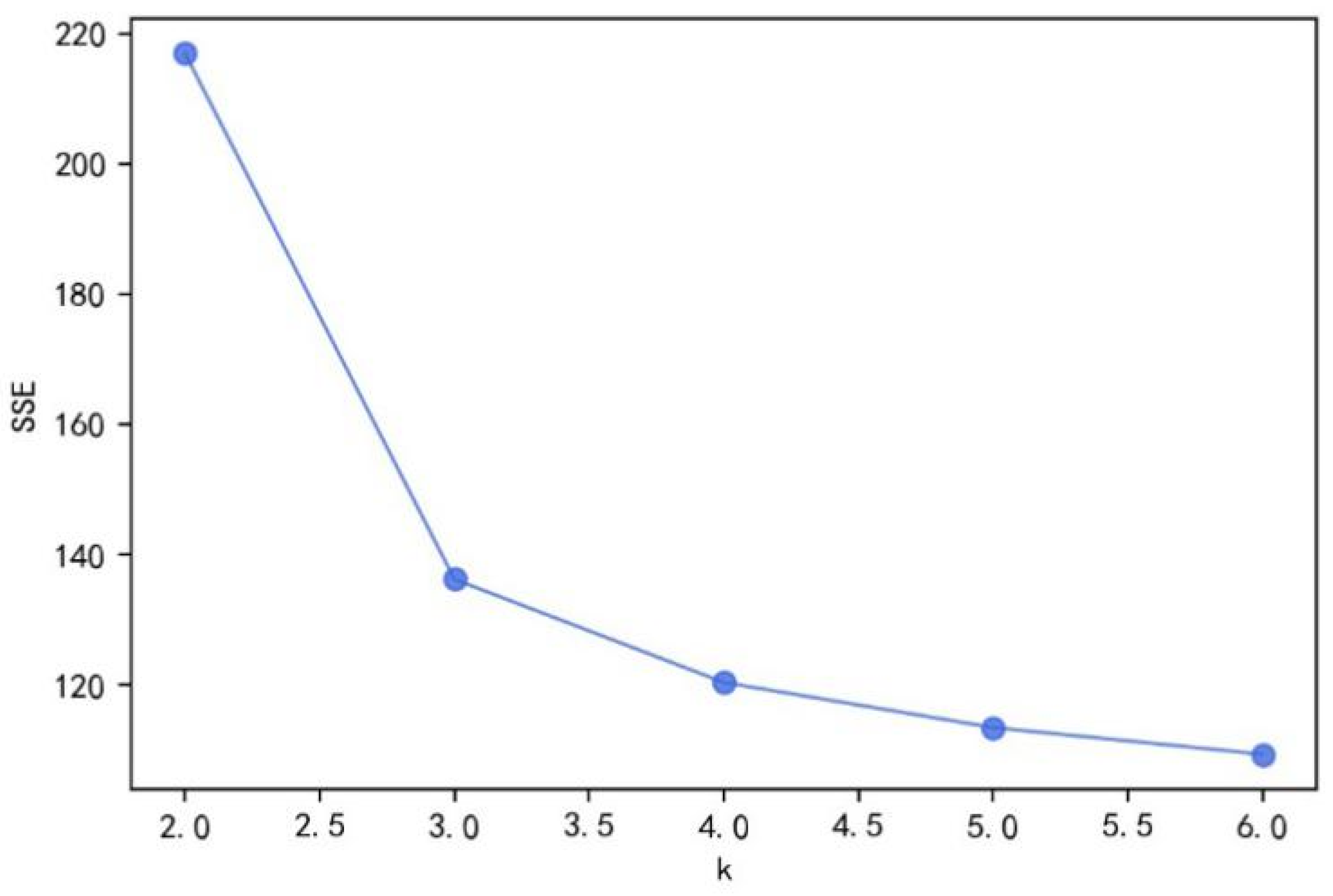
Since it contains 12 demand points in total, the value range of $k$ lies in [2, 4] according to the principle of $k\le \sqrt{n}$. Figure 3 shows the sum of the squares of error (SSE) when $k$ takes the values in [2, 6]. The optimal value is $k$ = 3.

After selecting the optimal $k$, clustering results are obtained according to the improved clustering algorithm, which is shown in

Table 4. The clustering results for the optimal k.

Regions	Central City	Covered Cities
Region 1	Xing’an	Tongliao, Chifeng, Hulun Buir
Region 2	Hohhot	Ulanqab, Baotou, Ordos, Xilin Gol
Region 3	Wuhai	Bayannur, Alxa

.

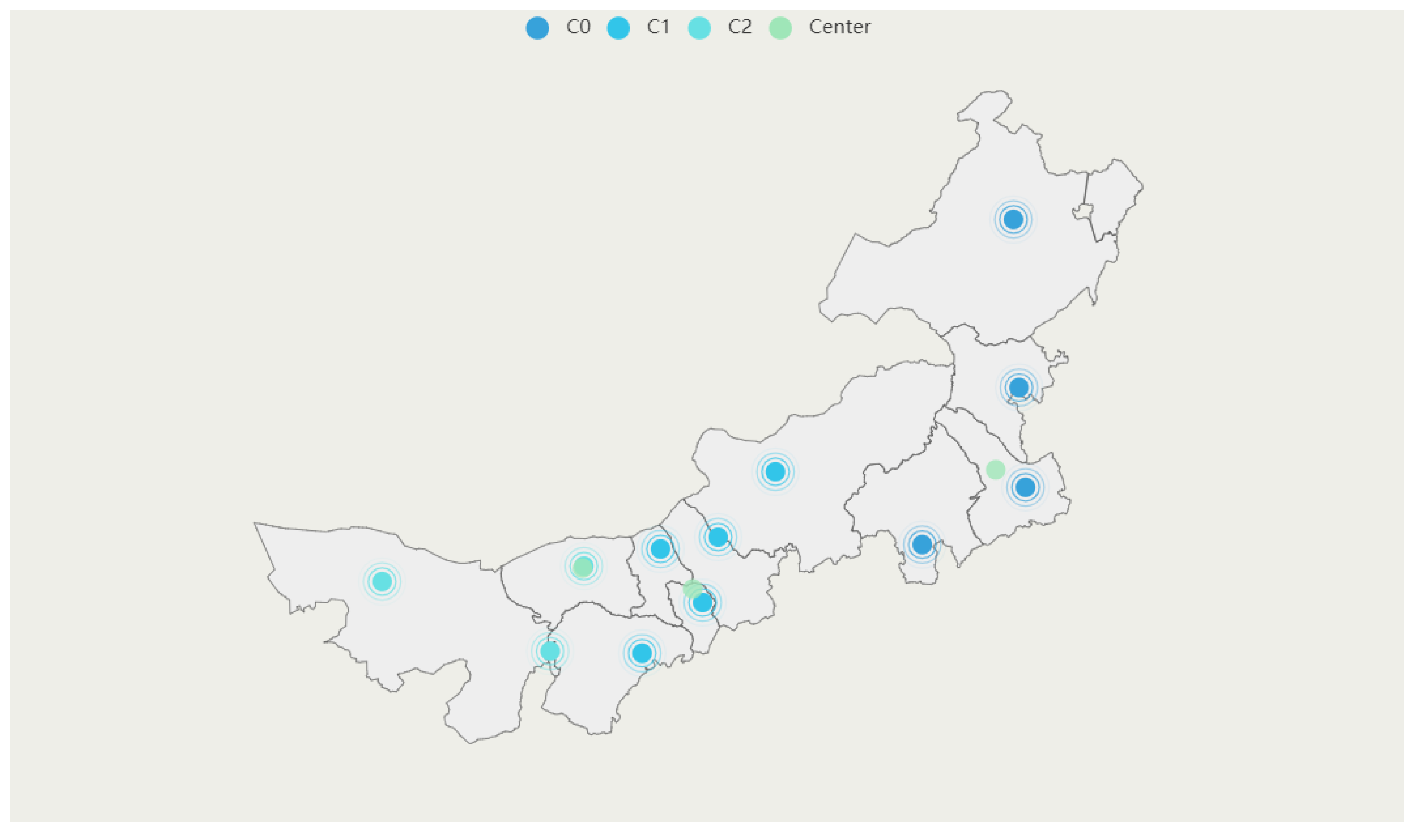
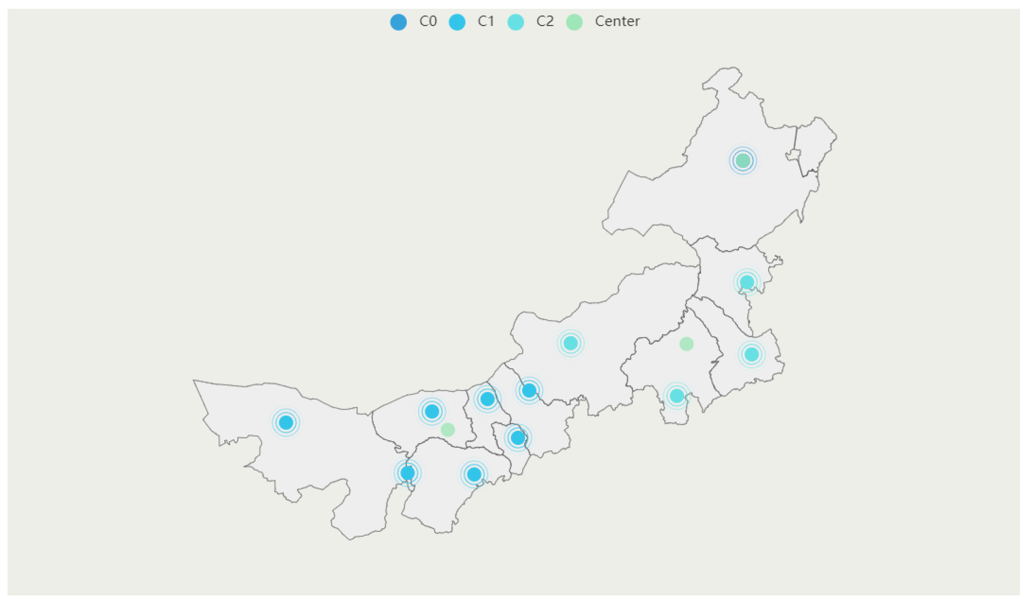
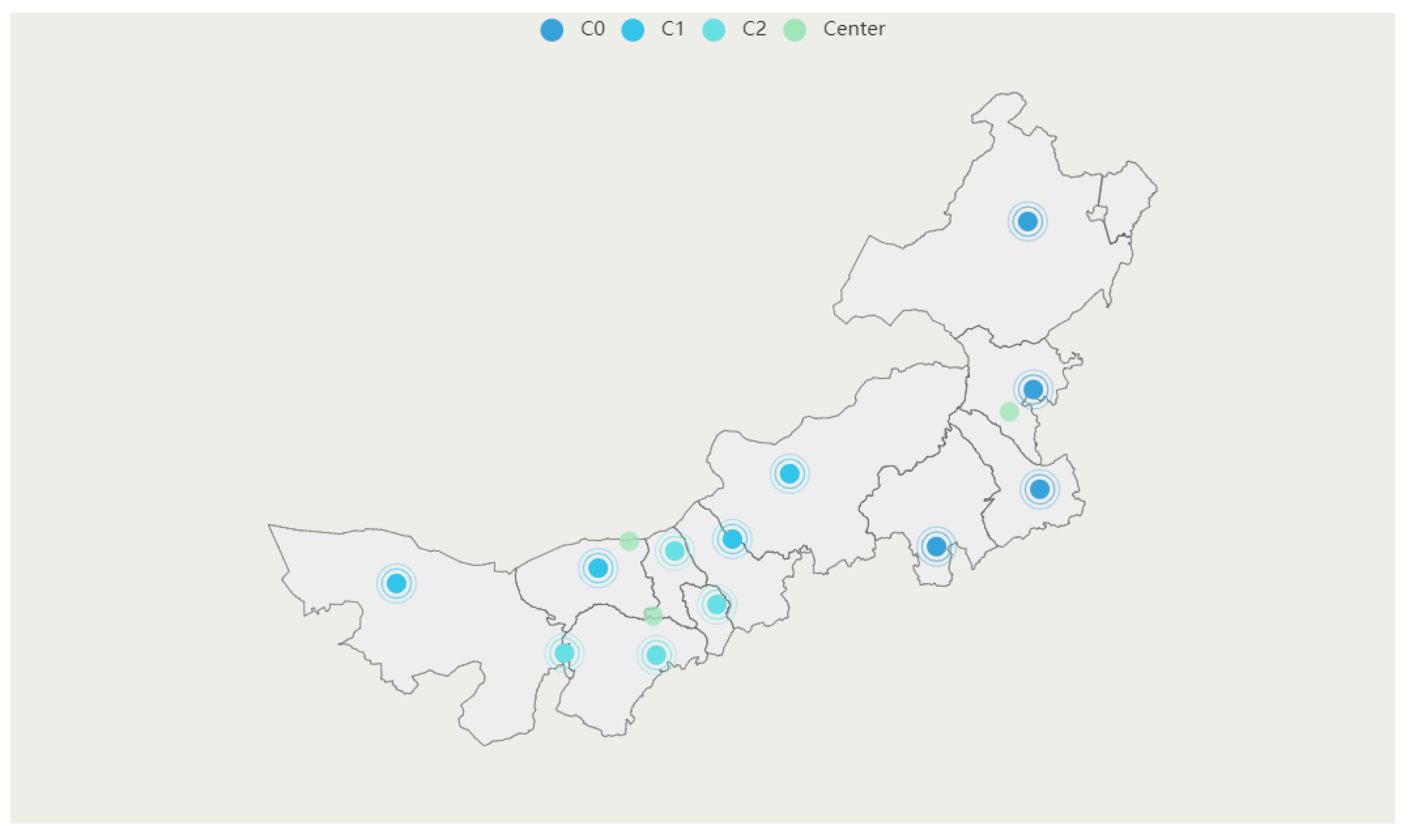
The result is modified by the center-of-gravity method. In this process, the permanent urban population is taken to represent the demand of each city. The modified results are shown in

Table 5. The location results for the 2SM.

Clustering	City Name	Longitude	Latitude	Demand
C0	Xing’an	122.0406	46.08926	75.13
	Tongliao	122.2505	43.65798	143.03
	Chifeng	118.8938	42.26083	211.42
	Hulun Buir	121.8592	50.18671	116.41
	Center 0	121.2842	44.08581
C1	Hohhot	111.7555	40.84842	265.5
	Ulanqab	112.2595	42.44243	100.29
	Baotou	110.3877	42.15471	232.48
	Ordos	109.7886	39.61359	165.04
	Xilin Gol	114.1209	44.03614	80.2
	Center 1	111.4345	41.1818
C2	Wuhai	106.801	39.6629	52.9
	Bayannur	107.8949	41.73579	91.77
	Alxa	101.339	41.36085	21.06
	Center 2	107.849	41.68704

and Figure 4. C0, C1, C2 and Center are in different colors in Figure 4.

A distribution center cannot be set up outside the city because of its infrastructure requirements. So, the distribution center is sited in a city closest to the location results for the 2SM. The results are shown in

Table 6. The final location results for the 2SM.

Regions	Central City	Covered Cities
Region 1	Tongliao	Chifeng, Hulun Buir, Xing’an
Region 2	Hohhot	Ulanqab, Baotou, Ordos, Xilin Gol
Region 3	Bayannur	Alxa, Wuhai

.

5. Evaluation

To evaluate the effectiveness of the two-stage model (2SM), the author makes a comparison on the results of it with three models’ based on the traditional $K$-means algorithm. For each model, $k$ is set as 3. Details are shown in the following.

Model 1: Geographic clustering model (GCM). This model considers only the geographical indicator. It takes the linear distance between cities as the similarity measurement. The distance between cities is computed based on the longitude and the latitude of each city. The location results are obtained by K-means clustering. The results are shown in

Table 7. The location results for the GCM.

Clustering	City Name	Longitude	Latitude	Demand
C0	Hulun Buir	121.8592	50.18671	116.41
	Center 0	121.8592	50.18671
C1	Hohhot	111.7555	40.84842	265.5
	Baotou	110.3877	42.15471	232.48
	Ulanqab	112.2595	42.44243	100.29
	Ordos	109.7886	39.61359	165.04
	Bayannur	107.8949	41.73579	91.77
	Wuhai	106.801	39.6629	52.9
	Alxa	101.339	41.36085	21.06
	Center 1	108.6037	41.11695
C2	Xing’an	122.0406	46.08926	75.13
	Tongliao	122.2505	43.65798	143.03
	Chifeng	118.8938	42.26083	211.42
	Xilin Gol	114.1209	44.03614	80.2
	Center 2	119.3265	44.01106

and Figure 5. C0, C1, C2 and Center are in different colors in Figure 5.

Model 2: Five-indicator clustering model (5ICM). This model contains five normalized indicators used in this paper: the longitude, the latitude, the per capita disposable income of urban residents, the permanent urban population and the population density. Euclidean distance is used to compute the distance between cities, the results are obtained by K-means clustering as shown in

Table 8. The location results for the 5ICM.

Clustering	City Name	Longitude	Latitude	Demand
C0	Hulun Buir	121.8592	50.18671	116.41
	Xing’an	122.0406	46.08926	75.13
	Tongliao	122.2505	43.65798	143.03
	Chifeng	118.8938	42.26083	211.42
	Center 0	121.261	45.5487
C1	Xilin Gol	114.1209	44.03614	80.2
	Ulanqab	112.2595	42.44243	100.29
	Bayannur	107.8949	41.73579	91.77
	Alxa	101.339	41.36085	21.06
	Center 1	108.9036	42.3938
C2	Hohhot	111.7555	40.84842	265.5
	Baotou	110.3877	42.15471	232.48
	Ordos	109.7886	39.61359	165.04
	Wuhai	106.801	39.6629	52.9
	Center 2	109.6832	40.5699

and Figure 6. C0, C1, C2 and Center are in different colors in Figure 6.

Model 3: Improved five-indicator clustering model (I5ICM). Based on the result of Model 2, this model incorporates the center-of-gravity method to obtain lower transportation costs. The results are shown in

Table 9. The location results for the I5ICM.

Clustering	City Name	Longitude	Latitude	Demand
C0	Hulun Buir	121.8592	50.18671	116.41
	Xing’an	122.0406	46.08926	75.13
	Tongliao	122.2505	43.65798	143.03
	Chifeng	118.8938	42.26083	211.42
	Center 0	121.2842	44.08581
C1	Xilin Gol	114.1209	44.03614	80.2
	Ulanqab	112.2595	42.44243	100.29
	Bayannur	107.8949	41.73579	91.77
	Alxa	101.339	41.36085	21.06
	Center 1	112.2504	42.44865
C2	Hohhot	111.7555	40.84842	265.5
	Baotou	110.3877	42.15471	232.48
	Ordos	109.7886	39.61359	165.04
	Wuhai	106.801	39.6629	52.9
	Center 2	110.9376	41.0485

and Figure 7. C0, C1, C2 and Center are in different colors in Figure 7.

The total transportation costs of the four models are shown in

Table 10. The transportation costs of the four models.

	GCM	5ICM	I5ICM	2SM
Transportation cost	3864.2391	4100.9813	3539.9559	3220.9834

.

As shown in Table 10, the 2SM proposed in this research has the lowest total transportation cost. Furthermore, compared with the three traditional models, the following conclusions can be drawn:

• Compared with the result of the geographic clustering model (GCM), clustering with five indicators (5ICM) has an increase in cost, this indicates that if the distance function or algorithm is not adjusted, the result will be worse than the original method.
• Using the center-of-gravity method to modify the clustering with five indicators (I5ICM) significantly reduces the cost.
• If the distance function is modified reasonably and the algorithm is improved into the two-stage model (2SM) proposed in this study, the cost will be further reduced.

6. Results and Conclusions

In this research, a two-stage location selection model based on an improved clustering algorithm and the center-of-gravity method is proposed for an MFLP arising from a real-world problem. This methodology is proved to be effective and contributing to future logistics system planning strategy researches. The following conclusions are drawn as follows.

First, the more indicators introduced into LP, the more realistic the research becomes. In this paper, three socio-economic indicators, namely, economy development, traffic congestion degree and total logistics demand, are introduced in defining a distance function used in clustering, each of which could affect the decision on the site of a distribution center. Different from most of the existing researches, which only used spatial indicators, this research introduces three socio-economic indicators to evaluate a city’s potential to accommodate a distribution center, described as the logistics-level score. This method provides a more comprehensive perspective for decision-makers to choose proper sites for distribution.

Second, an improved clustering algorithm is used to divide demand points into different regions. The improved algorithm redefines the traditional distance function, which could not reflect the distance result caused by the socio-economic indicators. The improved distance function takes both the positive effect of the three socio-economic indicators and the passive effect caused by the spatial indicators into consideration, and proved to be more effective than GCM, 5ICM and I5ICM in the case study.

Third, based on the methodology discussed above, this research divides 12 cities in Inner Mongolia into 3 regions and selects 1 city for each region as the regional distribution center. This is consistent with the government’s current logistics center planning strategy. Such consistency indicates that this methodology could be used as an optional reference for local governments’ logistics planning.

The limitation of this paper may lie in the selection of the clustering indicators. Although three socio-economic indicators are introduced in the 2SM, it is still impossible to describe the complexity of the logistics in real world. This means more socio-economic indicators or even more kinds of indicators should be introduced into LP researches. Besides, during the SFLP process, the author takes only the total transportation cost as the final objective and omits some other influential decision making factors. In subsequent research, other objectives/constraints such as carbon emission reduction and sustainable development can be added to the existing research.

References

- Ozmen, M.; Aydogan, E.K. Robust multi-criteria decision making methodology for real life logistics center location problem. Artif. Intell. Rev. 2020, 53, 725–751. [Google Scholar] [CrossRef]
- Zhuge, D.; Yu, S.; Zhen, L.; Wang, W. Multi-period distribution center location and scale decision in supply chain network. Comput. Ind. Eng. 2016, 101, 216–226. [Google Scholar] [CrossRef]
- He, Y.; Wang, X.; Lin, Y.; Zhou, F.; Zhou, L. Sustainable decision making for joint distribution center location choice. Transp. Res. Part D Transp. Environ. 2017, 55, 202–216. [Google Scholar] [CrossRef]
- Zhang, H.; Beltran-Royo, C.; Wang, B.; Zhang, Z. Two-phase semi-lagrangian relaxation for solving the uncapacitated distribution centers location problem for B2C E-commerce. Comput. Optim. Appl. 2019, 72, 827–848. [Google Scholar] [CrossRef]
- Zhou, Y.; Xie, R.; Zhang, T.; Holguin-Veras, J. Joint distribution center location problem for restaurant industry based on improved k-means algorithm with penalty. IEEE Access 2020, 8, 37746–37755. [Google Scholar] [CrossRef]
- Zhang, S.; Chen, N.; She, N.; Li, K. Location optimization of a competitive distribution center for urban cold chain logistics in terms of low-carbon emissions. Comput. Ind. Eng. 2021, 154, 107120. [Google Scholar] [CrossRef]
- Pérez-Mesa, J.C.; Serrano-Arcos, M.M.; Jiménez-Guerrero, J.F.; Sánchez-Fernández, R. Addressing the location problem of a perishables redistribution center in the middle of Europe. Foods 2021, 10, 1091. [Google Scholar] [CrossRef]
- Fearon, D. Alfred Weber: Theory of the Location of Industries, 1909; Center for Spatially Integrated Social Science: CA, USA, 2006. [Google Scholar]
- Afsharian, M. The p-efficient problem in location analytics: Definitions, formulations, applications, and future research directions. Healthc. Anal. 2022, 2, 100014. [Google Scholar] [CrossRef]
- Chen, R. Optimal location of a single facility with circular demand areas. Comput. Math. Appl. 2001, 41, 1049–1061. [Google Scholar] [CrossRef]
- Zeferino, E.F.S.; Mpofu, K.; Makinde, O.A.; Ramatsetse, B.I.; Daniyan, I.A. FR/CoG multi-attribute-based comparison methods for selection of the location of a research institute. J. Facil. Manag. 2020, 18, 20–35. [Google Scholar] [CrossRef]
- Trivedi, A.; Singh, A. Facility location in humanitarian relief: A review. Int. J. Emerg. Manag. 2018, 14, 213–232. [Google Scholar] [CrossRef]
- Alizadeh, R.; Nishi, T. Hybrid set covering and dynamic modular covering location problem: Application to an emergency humanitarian logistics problem. Appl. Sci. 2020, 10, 7110. [Google Scholar] [CrossRef]
- Liu, Y.; Yuan, Y.; Shen, J.; Gao, W. Emergency response facility location in transportation networks: A literature review. J. Traffic Transp. Eng. (Engl. Ed.) 2021, 8, 153–169. [Google Scholar] [CrossRef]
- Ahmadi-Javid, A.; Seyedi, P.; Syam, S.S. A survey of healthcare facility location. Comput. Oper. Res. 2017, 79, 223–263. [Google Scholar] [CrossRef]
- De Vries, H.; Van de Klundert, J.; Wagelmans, A.P. The roadside healthcare facility location problem a managerial network design challenge. Prod. Oper. Manag. 2020, 29, 1165–1187. [Google Scholar] [CrossRef]
- Nasiri, M.M.; Mahmoodian, V.; Rahbari, A.; Farahmand, S. A modified genetic algorithm for the capacitated competitive facility location problem with the partial demand satisfaction. Comput. Ind. Eng. 2018, 124, 435–448. [Google Scholar] [CrossRef]
- Farahani, R.Z.; Asgari, N.; Heidari, N.; Hosseininia, M.; Goh, M. Covering problems in facility location: A review. Comput. Ind. Eng. 2012, 62, 368–407. [Google Scholar] [CrossRef]
- Alizadeh, R.; Nishi, T.; Bagherinejad, J.; Bashiri, M. Multi-period maximal covering location problem with capacitated facilities and modules for natural disaster relief services. Appl. Sci. 2021, 11, 397. [Google Scholar] [CrossRef]
- Sarker, B.R.; Wu, B.; Paudel, K.P. Optimal location for renewable gas production and distribution facilities: Resource planning and management. BioEnergy Res. 2022, 15, 650–666. [Google Scholar] [CrossRef]
- Cheng, C.; Adulyasak, Y.; Rousseau, L.M. Robust facility location under demand uncertainty and facility disruptions. Omega 2021, 103, 102429. [Google Scholar] [CrossRef]
- Zhu, T.; Boyles, S.D.; Unnikrishnan, A. Two-stage robust facility location problem with drones. Transp. Res. Part C Emerg. Technol. 2022, 137, 103563. [Google Scholar] [CrossRef]
- Cui, T.; Ouyang, Y.; Shen, Z.J.M. Reliable facility location design under the risk of disruptions. Oper. Res. 2010, 58 Pt 1, 998–1011. [Google Scholar] [CrossRef] [Green Version]
- Shang, X.; Yang, K.; Wang, W.; Wang, W.; Zhang, H.; Celic, S. Stochastic hierarchical multimodal hub location problem for cargo delivery systems: Formulation and algorithm. IEEE Access 2020, 8, 55076–55090. [Google Scholar] [CrossRef]
- Snyder, L.V.; Daskin, M.S. Reliability models for facility location: The expected failure cost case. Transp. Sci. 2005, 39, 400–416. [Google Scholar] [CrossRef] [Green Version]
- Wang, W.; Wu, S.; Wang, S.; Zhen, L.; Qu, X. Emergency facility location problems in logistics: Status and perspectives. Transp. Res. Part E Logist. Transp. Rev. 2021, 154, 102465. [Google Scholar] [CrossRef]
- Gargouri, M.A.; Hamani, N.; Mrabti, N.; Kermad, L. Optimization of the collaborative hub location problem with metaheuristics. Mathematics 2021, 9, 2759. [Google Scholar] [CrossRef]
- Akyuz, M.H.; Oncan, T.; Altınel, I.K. Branch and bound algorithms for solving the multi-commodity capacitated multi-facility Weber problem. Ann. Oper. Res. 2019, 279, 1–42. [Google Scholar] [CrossRef]
- Yang, Z.; Chen, H.; Chu, F.; Wang, N. An effective hybrid approach to the two-stage capacitated facility location problem. Eur. J. Oper. Res. 2019, 275, 467–480. [Google Scholar] [CrossRef]
- Silva, A.; Aloise, D.; Coelho, L.C.; Rocha, C. Heuristics for the dynamic facility location problem with modular capacities. Eur. J. Oper. Res. 2021, 290, 435–452. [Google Scholar] [CrossRef]
- Ozgun-Kibiroglu, C.; Serarslan, M.N.; Topcu, Y.I. Particle swarm optimization for uncapacitated multiple allocation hub location problem under congestion. Expert Syst. Appl. 2019, 119, 1–19. [Google Scholar] [CrossRef]
- Ramshani, M.; Ostrowski, J.; Zhang, K.; Li, X. Two level uncapacitated facility location problem with disruptions. Comput. Ind. Eng. 2019, 137, 106089. [Google Scholar] [CrossRef]
- Li, J.; Xiao, D.D.; Lei, H.; Zhang, T.; Tian, T. Using cuckoo search algorithm with q-learning and genetic operation to solve the problem of logistics distribution center location. Mathematics 2020, 8, 149. [Google Scholar] [CrossRef] [Green Version]
- Rostami, M.; Bagherpour, M. A lagrangian relaxation algorithm for facility location of resource-constrained decentralized multi-project scheduling problems. Oper. Res. 2020, 20, 857–897. [Google Scholar] [CrossRef]
- Iyigun, C.; Ben-Israel, A. A generalized Weiszfeld method for the multi-facility location problem. Oper. Res. Lett. 2020, 38, 207–214. [Google Scholar] [CrossRef]
- Esnaf, S.; Kuçukdeniz, T. A fuzzy clustering-based hybrid method for a multi-facility location problem. J. Intell. Manuf. 2009, 20, 259–265. [Google Scholar] [CrossRef]
- Kuçukdeniz, T.; Baray, A.; Ecerkale, K.; Esnaf, S. Integrated use of fuzzy c-means and convex programming for capacitated multi-facility location problem. Expert Syst. Appl. 2012, 39, 4306–4314. [Google Scholar] [CrossRef]
- Gupta, R.; Muttoo, S.K.; Pal, S.K. Fuzzy c-means clustering and particle swarm optimization based scheme for common service center location allocation. Appl. Intell. 2017, 47, 624–643. [Google Scholar] [CrossRef]
- Gao, X.; Park, C.; Chen, X.; Xie, E.; Huang, G.; Zhang, D. Globally optimal facility locations for continuous-space facility location problems. Appl. Sci. 2021, 11, 7321. [Google Scholar] [CrossRef]
- Pérez-Suárez, A.; Martínez-Trinidad, J.F.; Carrasco-Ochoa, J.A. A review of conceptual clustering algorithms. Artif. Intell. Rev. 2019, 52, 1267–1296. [Google Scholar] [CrossRef]
- Ushakov, A.V.; Vasilyev, I. Near-optimal large-scale k-medoids clustering. Inf. Sci. 2021, 545, 344–362. [Google Scholar] [CrossRef]
- Wang, T.; Li, Q.; Bucci, D.J.; Liang, Y.; Chen, B.; Varshney, P.K. K-medoids clustering of data sequences with composite distributions. IEEE Trans. Signal Process. 2019, 67, 2093–2106. [Google Scholar] [CrossRef]
- Bai, H.; Feng, F.; Wang, J.; Wu, T. A combination prediction model of long-term ionospheric foF2 based on entropy weight method. Entropy 2020, 22, 442. [Google Scholar] [CrossRef] [PubMed] [Green Version]
- Lin, H.; Du, L.; Liu, Y. Soft decision cooperative spectrum sensing with entropy weight method for cognitive radio sensor networks. IEEE Access 2020, 8, 109000–109008. [Google Scholar] [CrossRef]