Multimode Process Monitoring Based on Modified Density Peak Clustering and Parallel Variational Autoencoder

Abstract

Clustering algorithms and deep learning methods have been widely applied in the multimode process monitoring. However, for the process data with unknown mode, traditional clustering methods can hardly identify the number of modes automatically. Further, deep learning methods can learn effective features from nonlinear process data, while the extracted features cannot follow the Gaussian distribution, which may lead to incorrect control limit for fault detection. In this paper, a comprehensive monitoring method based on modified density peak clustering and parallel variational autoencoder (MDPC-PVAE) is proposed for multimode processes. Firstly, a novel clustering algorithm, named MDPC, is presented for the mode identification and division. MDPC can identify the number of modes without prior knowledge of mode information and divide the whole process data into multiple modes. Then, the PVAE is established based on distinguished multimode data to generate the deep nonlinear features, in which the generated features in each VAE follow the Gaussian distribution. Finally, the Gaussian feature representations obtained by PVAE are provided to construct the statistics $H^2$, and the control limits are determined by the kernel density estimation (KDE) method. The effectiveness of the proposed method is evaluated by the Tennessee Eastman process and semiconductor etching process.

1. Introduction

With the increasing demands for production efficiency, stable system, and safe operation in modern industry, fault detection and diagnosis (FDD) has received more and more attention. In recent years, data-driven methods, especially the multivariate statistical process monitoring (MSPM) methods, have become very popular. Principal component analysis (PCA) and partial least squares (PLS) are two major MSPM methods [1,2,3,4]. To solve the dynamic problem, a novel dynamic weight principal component analysis (DWPCA) algorithm and a hierarchical monitoring strategy were proposed [5]. In order to handle missing or corrupted data, a variational Bayesian PCA (VBPCA)-based methodology was presented and applied in wastewater treatment plants (WWTPs) [6]. For the large-scale process data, Zhang et al. proposed a decentralized fault diagnosis approach based on multiblock kernel partial least squares (MBKPLS) [7].

Many MSPM methods have also been proposed for processes with multiple operating conditions. For the multiple working modes and plant-wide characteristics, Chang et al. proposed an on-line operating performance evaluation approach based on a multiple three-level multi-block hybrid model [8]. Peng et al. proposed a multiple PLS model and applied it to quality-related prediction and fault detection [9]. However, it should be noted that traditional MSPM methods assume that data obey a single-peak distribution. The local process information is not taken into consideration. This may lead to erroneous and costly monitoring results [10].

In recent years, many methods have been developed to improve the performance of multimode process monitoring. One intuitive idea is the global model. For example, local least squares support vector regression (LSSVR) and two-step independent component analysis–principal component analysis (ICA–PCA) were introduced for the multimode on-line monitoring [11]. Song and Shi presented a global model based on temporal–spatial global locality projections for multimode process [12]. However, most global modeling methods are hardly able to represent each operating mode precisely due to the statistical averaging. The local modeling methods are also developed to monitor the status of a multimode process. A local neighborhood standardization strategy integrating with PCA (LNS-PCA) was developed for multimode fault detection [13]. A fault detection method based on adaptive Mahalanobis distance and k-nearest neighbor (MD-kNN) was proposed and applied in semiconductor manufacturing [14]. Deng et al. proposed a local neighborhood similarity analysis method for monitoring processes [15]. However, these methods require the nearest neighbor searching on each historical sample, which is a high computational load. Meanwhile, the prior knowledge to select the number of neighbors is difficult to obtain. Another common multimode process monitoring method is based on mixture model, which is suitable to represent the data sources driven by different operating modes. Yu and Qin proposed a probabilistic approach based on finite Gaussian mixture model (FGMM) and Bayesian inference for fault detection under different modes [16]. Taking the dynamic characteristics of industrial process into consideration, an adaptive Gaussian mixture model (GMM) using some prior knowledge for adaptive updating was proposed [17]. A novel monitoring strategy, which combines the advantages of multiple modeling strategies and GMM, was proposed for multimode processes [18]. In addition, the clustering method is adopted to separate the different process modes. Khediri et al. presented a procedure based on kernel k-means clustering and support vector domain description (SVDD) to identify the nonlinear process modes and detect faults, respectively [19]. The fuzzy c-means (FCM) clustering method was employed to partition the multimode process data into multiple clusters [20]. A novel monitoring strategy based on locality preserving projection (LPP) and FCM was proposed for extracting the multimode feature [21]. Luo et al. proposed a mode partition method based on the warped k-means clustering algorithm [22]. However, similar to the GMM-based methods, aforementioned clustering methods must manually set the cluster numbers in advance [23].

Density peaks clustering (DPC) is a novel clustering algorithm proposed by Rodriguez and Laio in 2014 [24]. It provides a simple way to find the cluster centers and an efficient manner to group non-center data. DPC has been widely studied and applied in the field of the multimode process monitoring. For example, a hierarchical mode division based on hierarchical density peaks clustering and hybrid geodesic distance was presented to extract more available information from the multimode process data, which can improve the adaptability of industrial processes with uncertainty [25]. A kNN-based modified DPC method was proposed and applied to multimode process monitoring [26]. The DPC can find the cluster centers for each operation mode according to the distribution characteristics of the process data. Nevertheless, there are still some unresolved problems existing in the original DPC to hinder it from becoming a reliable clustering algorithm: (1) The magnitudes of local density in different modes are inconsistent, which may lead to the wrong selection of cluster centers, and (2) there is not a valid criterion to determine the optimal number of cluster centers automatically.

In the past decade, deep learning has been widely studied due to its powerful feature extracting and representation learning ability. Among various of deep learning methods, autoencoder (AE) plays a central role. An anomaly detection method based on sequence gated recurrent units (SGRU) and AE was proposed for industrial multimode process [27]. A monitoring scheme based on GMM and stacked denoising autoencoder (GMM-SDAE) was constructed to identify the mode and extract feature from monitoring data [28]. Since AE is a self-reconstruction network, most AE-related methods cannot ensure the distribution characteristics of extracted features. This may cause improper control limit, which leads to inferior monitoring performance. Recently, variational autoencoder (VAE) has attracted increasing attention in the process monitoring domain. A significant advantage of VAE is that the learned hidden features follow the Gaussian distribution. Associated with the nonlinear reflection of neural network, VAE is suitable for the feature learning in industrial process monitoring. A nonlinear process monitoring method based on VAE was proposed to tackle the Gaussian assumption problem [29]. For the multivariate fault isolation problem, a process monitoring framework was proposed using VAE and branch-bound algorithm [30]. However, the VAE-based method is limited by the Gaussian distribution assumption of the hidden feature, which is not suitable for data with multiple mixture distributions [31,32].

Owing to the diversity of data distribution in different mode, the local density in DPC is inappropriate as a measure for selecting cluster centers. In addition, the number of the cluster centers in DPC is usually selected manually. For the multimode process dataset without mode information, improper number of modes may degrade the modeling and monitoring performance. Meanwhile, VAE shows good performance in the single-mode process monitoring, but it cannot model well for multimode data.

To address the problem above, this paper proposes a multimode process monitoring method based on modified density peak clustering and parallel variational autoencoder (MDPC-PVAE). The MDPC-PVAE can fully extract the informative nonlinear feature from the multimode process data. The MDPC can effectively identify and divide the process data in different modes, and the learned features by PVAE follow the Gaussian distribution. The proposed method contains two phases: mode identification and feature generation. In the mode identification phase, the MDPC is proposed to identify the mode information and determine the process data in each mode. As a modified decision graph measure, local density ratio is presented to unify the local density peak and reduce the local density diversity in different clusters. Moreover, total entropy estimation is employed as a criterion to determine the optimal number of cluster centers. In the feature generation phase, the PVAE is presented to learn the multimode data and generate representative features for process monitoring. It is constituted by multiple VAEs, in which the process data of a mode is utilized for constructing a VAE. The learned features in each VAE follows the Gaussian distribution. Finally, the monitoring statistics $H^2$ are constructed based on the Gaussian features generated by PVAE. The corresponding control limits are determined by the kernel density estimation (KDE) method. Different from most multi-model methods, in the on-line monitoring, the new sample is directly fed into the MDPC-PVAE without determining which mode the sample belongs to in advance.

The remainder of this paper is organized as follows: in Section 2, DPC and VAE are briefly introduced. In Section 3, the proposed MDPC-PVAE and its multimode monitoring procedure are described. In Section 4, the performance of proposed method is compared with some related multimode process monitoring methods on the Tennessee Eastman (TE) process and semiconductor etching (SE) process. Finally, conclusions are drawn in Section 5.

2. Preliminaries

In this section, we briefly review the basic concepts related to DPC and VAE.

2.1. Density Peak Clustering

DPC is a simple density-based clustering algorithm. Different from traditional center-based clustering algorithms such as k-means and FCM, DPC is able to detect non-spherical clusters and to recognize the correct number of clusters by artificial observation. There are two basic assumptions about cluster centers. First, the cluster center has higher local density than that of their neighbor points. Second, the distances between cluster centers are relatively large. For a dataset $X\in R^{n\times m}$ with n samples and m variables, the Euclidean distance $d_{ij}$ between two samples $x_i$ and $x_j$ is calculated as follows:

$$d_{ij}=\parallel x_i-x_j{\parallel }^2,$$

(1)

For a sample $x_i$, two important measures, i.e., the local density ${\rho }_i$ and the minimum distance ${\delta }_i$ are defined to select the cluster centers. The local density ${\rho }_i$ is defined as:

$${\rho }_i={{\displaystyle \sum }}_j\chi \left(d_{ij}-d_c\right),$$

(2)

where, in $\chi \left(x\right)$, if $x<0$, $\chi \left(x\right)=1$. Otherwise, $\chi \left(x\right)=0$. $d_c$ is a cutoff distance. ${\rho }_i$ presents the number of data points that have a distance to $x_i$ less than $d_c$. The local density can be also calculated using the Gaussian function:

$${\rho }_i={{\displaystyle \sum }}_{j}exp\left(-\frac{d_{ij}^2}{d_c^2}\right),$$

(3)

The minimum distance ${\delta }_i$ of data point $x_i$ is measured by calculating the minimum distance between $x_i$ and the other data points with higher local density. It is expressed as:

$${\delta }_i=\left\{\begin{array}{c}\underset{j:{\rho }_i<{\rho }_j}{\min }\left(d_{ij}\right), if \exists j, s.t. {\rho }_i<{\rho }_j \\ \underset{j}{\max }\left(d_{ij}\right), otherwise\end{array}\right.,$$

(4)

Then, the measures ${\rho }_i$ and ${\delta }_i$ are used to generate a two-dimensional decision graph. Generally, the cluster centers are manually selected according to the location of measures. The cluster centers always locate on the upper-right corner. In some studies, the cluster centers can also be determined by the composite indicator ${\epsilon }_i$ as:

$${\epsilon }_i={\rho }_i{\delta }_i, i\in I,$$

(5)

Obviously, the data point with larger ${\epsilon }_i$ is more likely the cluster center. After the cluster centers are determined, each remaining data point is assigned to the cluster to which its nearest neighbor with higher local density belongs.

2.2. Variational Autoencoder

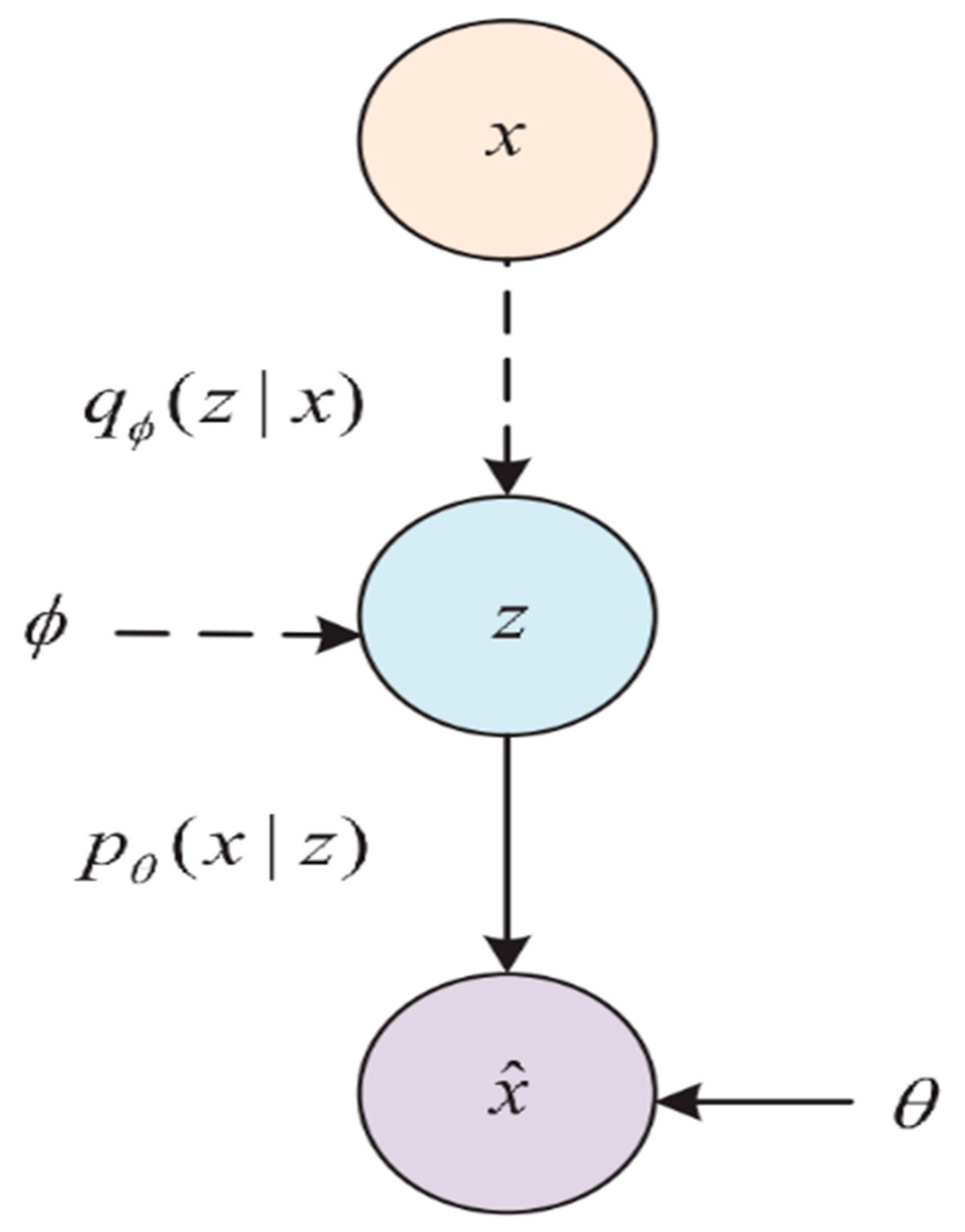
The VAE is a stochastic generative model that can solve the inference problem. It can replace the latent representation of given data with stochastic variables and force the latent variables to obey an expected Gaussian distribution. The basic structure of VAE is shown in Figure 1. Given the dataset $X$, the goal of VAE is to generate the data $\widehat{x}$ from the unobserved latent variable $z$ by optimizing the network parameters $\theta$. To make the generated data $\widehat{x}$ similar to the original data $x$ with high probability, we should maximize the likelihood $p_{\theta }\left(x\right)$:

$$p_{\theta }\left(x\right)=\int p_{\theta }(x|z)p_{\theta }\left(z\right)dz$$

(6)

The log likelihood $\log p_{\theta }\left(x^i\right)$ can be expressed as:

$$\log p_{\theta }\left(x^i\right)={\mathsf{{\rm E}}}_{q_{\varphi }(z|x^i)}\left(\log p_{\theta }(x^i|z)\right)-D_{KL}(q_{\varphi }(z|x^i)\parallel p_{\theta }\left(z\right))+D_{KL}(q_{\varphi }(z|x^i)\parallel p_{\theta }(z\parallel x^i)),$$

(7)

where $p_{\theta }(x^i|z)$ is the decoder, $q_{\varphi }(z|x^i)$ is the encoder, $\theta$ and $\varphi$ are the network parameters, and $D_{KL}$ is the Kullback–Leibler (KL) divergence. In Equation (7), $p_{\theta }(z\parallel x^i)$ is intractable, and KL divergence is non-negative. VAE considers an approximation of the marginal likelihood, denoted as evidence lower bound (ELBO), which is a lower bound of the log likelihood as:

$$\mathcal{L}\left(\theta ,\varphi ;x^i\right)={\mathsf{{\rm E}}}_{q_{\varphi }(z|x^i)}\left[\log p_{\theta }(x^i|z)\right]-D_{KL}(q_{\varphi }(z|x^i)\parallel p_{\theta }\left(z\right)),$$

(8)

The ELBO consists of two terms. The first term is the reconstruction error, which is the same as the training objective of an autoencoder. The KL divergence term is a distance measure between the probability distribution of generated data and expected Gaussian distribution. Through maximizing the ELBO, the network parameters $\theta$ and $\varphi$ are optimized. Stochastic gradient descent algorithm is used for the network training.

3. Multimode Process Monitoring Based on MDPC-PVAE

This section introduces the detail of the proposed MDPC-PVAE and its multimode process monitoring procedure.

3.1. MDPC-PVAE

In the original DPC, the cluster centers are selected from local density peaks. However, for the multimode problem, the data distribution characteristics between different mode are various. DPC only focuses on value of local density and neglects if the density is really large in absolute magnitude. It means that a data point A in the higher density and wider coverage area is more likely becoming a cluster center than the data point B in a low-density and narrow coverage area even if the data point B has the highest local density in its area. Considering density diversity in a different area, namely a new decision graph measure, the local density ratio ${\gamma }_i$ is proposed to handle the density differences as:

$${\gamma }_i=\frac{1}{M}{{\displaystyle \sum }}_{j=1}^M\frac{{\rho }_i}{{\rho }_j}={{\displaystyle \sum }}_{j=1}^{{\rho }_i}\frac{1}{{\rho }_j}, {\rho }_j\in S_i,$$

(9)

where $S_i$ is the set containing the M data points with distances to $x_i$ less than $d_c$. If data point $x_i$ is a local density peak, all its M neighbor points have lower local density than ${\rho }_i$, i.e., ${\rho }_i>{\rho }_j$, and ${\gamma }_i>1$. The local density ratio can reduce the influence from large density differences across clusters.

After the ${\gamma }_i$ for each data point has been calculated, integrated with the previously mentioned measure ${\delta }_i$, the candidate cluster centers $C_{ca}$ are obtained through introducing the conditions as follows:

$${\left\{C_{ca}\left({\gamma }_{{ca}_n},{\delta }_{{ca}_n}\right)\right\}}_{n=1}^P=\{x\left({\gamma }_i,{\delta }_i\right)|{\gamma }_i>T_{\gamma }\cap {\delta }_i>T_{\delta }\}, i=1, 2, \dots , N,$$

(10)

where $T_{\gamma }$ and $T_{\delta }$ are the thresholds for ${\gamma }_i$ and ${\delta }_i$, respectively. $T_{\gamma }$ can remove the non-center data with low local density ratio. $T_{\delta }$ is used for eliminating the redundant data with high local density ratio. In this study, $T_{\gamma }$ is set to 1, and the average value of ${\delta }_i$ is taken as the threshold $T_{\delta }$. After that, the composite indicator ${\epsilon }_i^{\prime }$ about $C_{ca}$ is defined as:

$${\epsilon }_i^{\prime }={\gamma }_{{ca}_i}{\delta }_{{ca}_i}, i=1, 2, \dots , P,$$

(11)

The selection order of cluster centers is determined by the value of composite indicator ${\epsilon }_i^{\prime }$. We define ${\left\{s_i\right\}}_{i=1}^P$ as the descending order index set of ${\left\{{\epsilon }_i^{\prime }\right\}}_{i=1}^P$; that is:

$${\epsilon }_{s_1}\ge {\epsilon }_{s_2}\ge \dots \ge {\epsilon }_{s_P}$$

(12)

Then, we can sort all the data points corresponding to the ${\left\{s_i\right\}}_{i=1}^P$ as the selection sequence of cluster centers $C_i$:

$${\left\{C_i\right\}}_{i=1}^P={\left\{C_{{ca}_{s_i}}\right\}}_{i=1}^P$$

(13)

After the selection sequence of cluster centers is obtained, entropy estimation is employed to determine the number of cluster centers. Renyi entropy is a nonparametric estimation method that reflects the similarity or dissimilarity metric between data in the same space. For a stochastic variable x with a probability density function f(x), its Renyi entropy is:

$$E_{\alpha }\left(x\right)=\frac{1}{1-\alpha }\log \int f^{\alpha }\left(x\right)dx, \alpha >0, \alpha \ne 1,$$

(14)

where α is the information order. If α = 2, the Renyi quadratic entropy is given as:

$$E_R\left(x\right)=-\log \int f^2\left(x\right)dx$$

(15)

Equation (15) can be directly estimated by the Parzen window density estimation with a multi-dimensional Gaussian window function. Probability density function estimation of a cluster with the center $C_k$ can be represented as follows:

$$f\left(x\right)=\frac{1}{N_k}{{\displaystyle \sum }}_{i=1}^{N_k}G\left(x-x_i, {\sigma }^{2}I\right),$$

(16)

where $N_k$ is the number of data points belonging to the cluster with center $C_k$, and G is the Gaussian window function with covariance matrix ${\sigma }^{2}I$. G is represented as follows:

$$G\left(x-x_i, {\sigma }^{2}I\right)=\frac{1}{{\left(2\pi \right)}^{M/2}{\sigma }^M}\exp \left(\frac{-{\left(x-x_i\right)}^T\left(x-x_i\right)}{2{\sigma }^2}\right),$$

(17)

where M is the dimension number of x. The scale parameter governs the width of the Parzen window. By substituting (17) into (16), the entropy formula of cluster with center $C_k$ can be obtained as follows:

$$E\left(C_k\right)=-\log V\left(C_k\right) ,$$

(18)

where $V\left(C_k\right)$ can be expressed as follows:

$$V\left(C_k\right)=\frac{1}{N_k^2}{\displaystyle \sum }_{i=1}^{N_k}{\displaystyle \sum }_{j=1}^{N_k}G\left(x_j-x_i, 2{\sigma }^{2}I\right)$$

(19)

Assume that there are R clusters in the dataset; the first R elements in the selection sequence of cluster center, i.e., $\left\{C_1, C_2, \dots , C_R\right\}$, are chosen as the cluster centers. Each remaining point is assigned to the cluster to which its nearest neighbor with higher density belongs. The total entropy can be calculated as follows:

$$\tilde{E}\left(R\right)={\displaystyle \sum }_{n=1}^{R}E\left(C_n\right), R\le P$$

(20)

Note that, in calculating the $E\left(C_n\right)$, the kernel size $\sigma$ in the Gaussian window function is unified and consistent with that of $\tilde{E}\left(1\right)$. Obviously, if all the data points are assigned to the proper clusters, the data in each cluster may be more similar, and then, the total entropy becomes lower. The number of cluster centers $N_c$ can be obtained through finding the minimum total entropy in different combination of cluster centers:

$$N_c=\arg \min \left(\tilde{E}\left(R\right)\right), R=1, 2, \dots , P$$

(21)

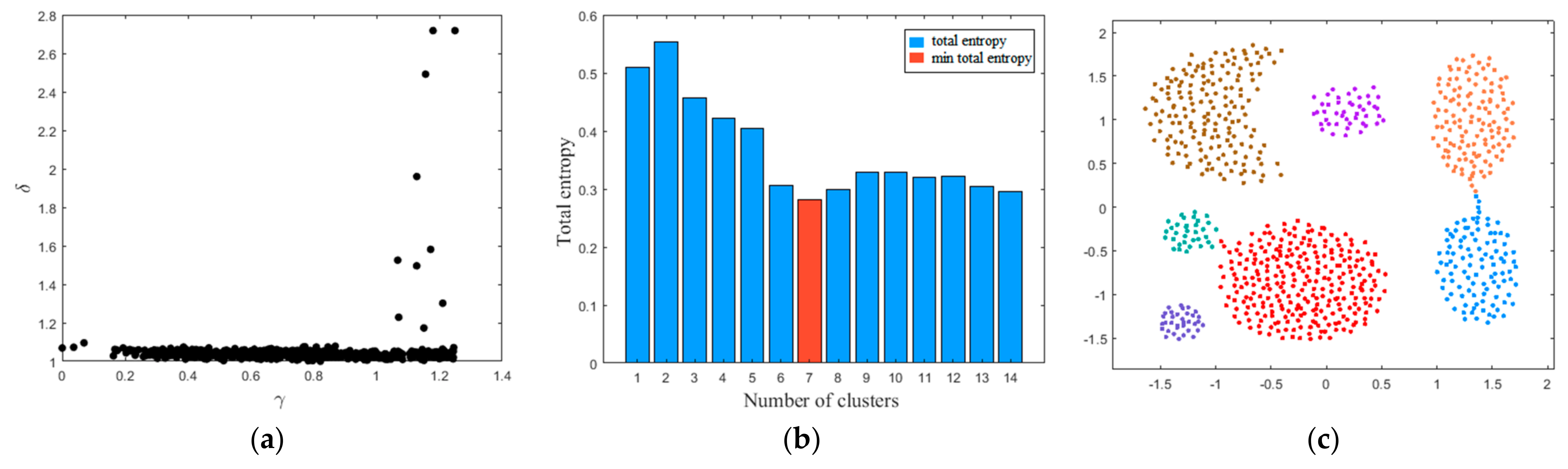
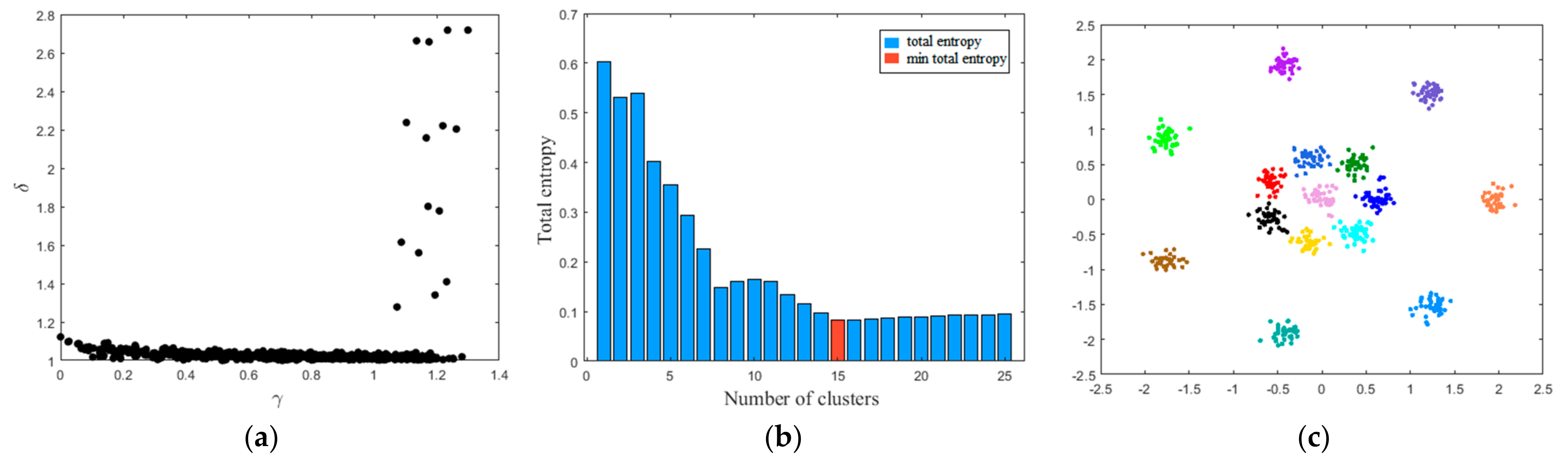
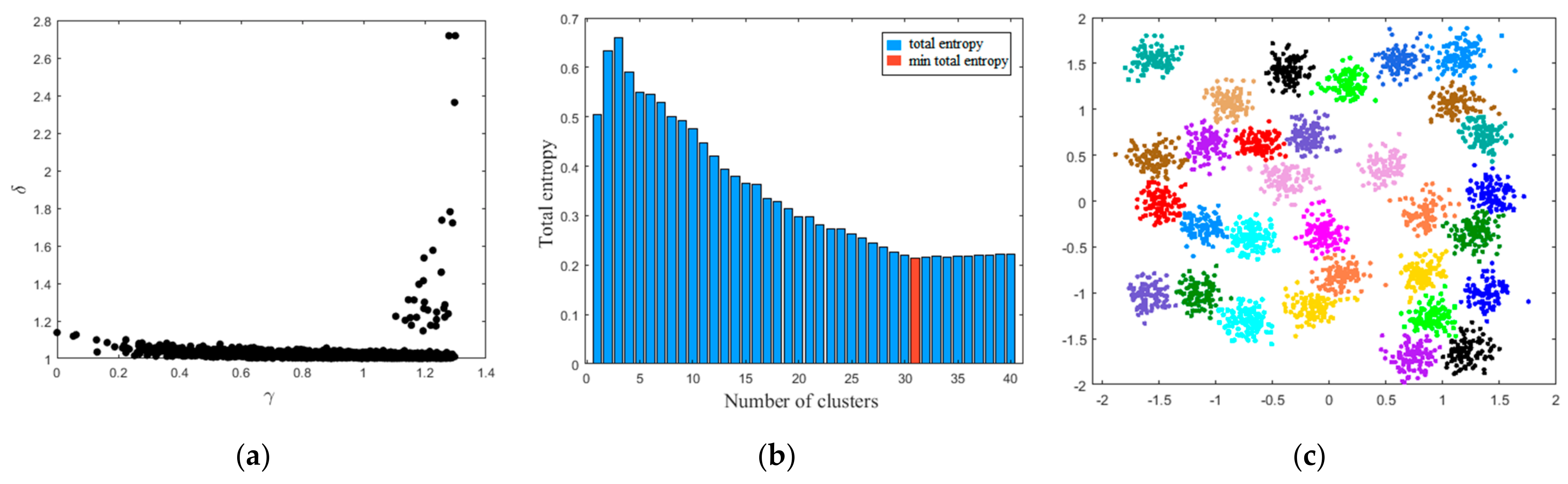
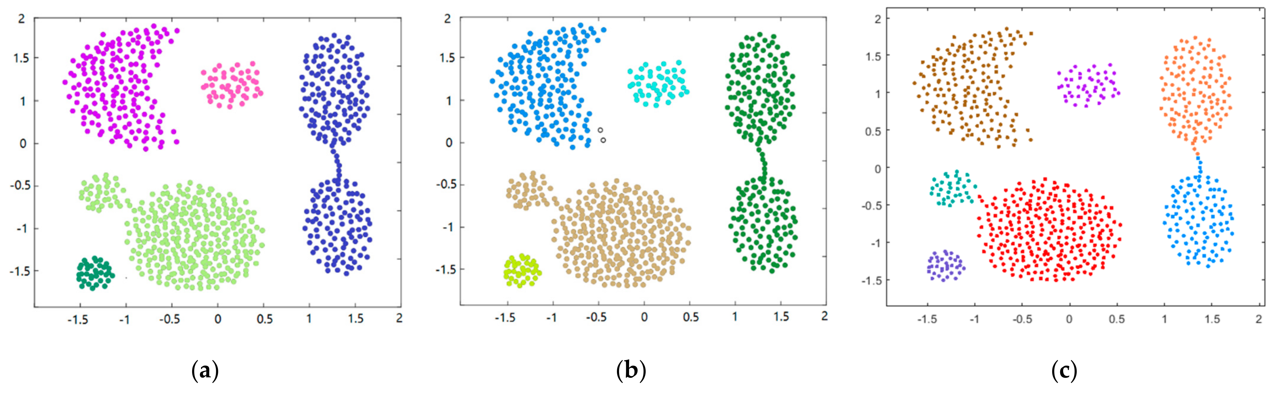
The overall procedures of MDPC are described in Algorithm 1. Considering that the multimode data usually show the multi-clusters distribution characteristics, three synthetic datasets (i.e., Aggregation, R15, and D31) are adopted to verify the clustering effect of MDPC [33]. The $\gamma -\delta$ decision graph, total entropy with different number of clusters, and visual clustering result on the three synthetic datasets are shown in Figure 2, Figure 3 and Figure 4. The clustering results show that MDPC shows good clustering performance. Through introducing local density ratio, the cluster centers can be found exactly. Entropy estimation determines the optimal number of clusters. The clustering results of DPC, DBSCAN, and MDPC on the Aggregation dataset re shown in Figure 5. It can be seen that MDPC can find the accurate cluster center. DPC and DBSCAN can only determine cluster centers with the high local density and ignore the local density peak.

Algorithm 1. MDPC.

Input: Dataset $X=\left\{x_1, x_2, \dots , x_N\right\}.$

Output: Cluster centers $C=\left\{C_1, C_2, \dots ,C_{N_c}\right\}.$

1: Calculate the distance $d_{ij}$ between data point $x_i$ and $x_j$.

2: Assign the cut-off distance $d_c$.

3: Calculate the local density ${\rho }_i$ of each data point.

4: Calculate the local density ratio ${\gamma }_i$ and minimum distance ${\delta }_i$ of each data point.

5: Assign the thresholds $T_{\gamma }$ and $T_{\delta }$.

6: Determine the candidate cluster center set ${\left\{C_{{ca}_i}\right\}}_{i=1}^P$.

7: Calculate the composite indicator ${\epsilon }_i^{\prime }$.

8: Sort the ${\epsilon }_i^{\prime }$ in descending order and record the index order ${\left\{s_i\right\}}_{i=1}^P$.

9: Determine selection sequence of cluster centers ${\left\{C_i\right\}}_{i=1}^P$.

10: for R = 1:P Calculate the total entropy $\tilde{E}\left(R\right)$.  End

11: Find the minimum $\tilde{E}\left(R\right)$, obtain the number of cluster centers $N_c$, and determine the cluster centers ${\left\{C_i\right\}}_{i=1}^{N_c}$.

12: Return $C=\left\{C_1, C_2, \dots ,C_{N_c}\right\}$.

Based on the MDPC, the whole multimode process is distinguished as multiple single modes. The process data X are divided in $N_c$ data subsets $\left\{X_1, X_2,\dots , X_{N_c}\right\}$. Since there are many differences between modes in the input profiles, conditions, process characteristics, and control strategy, traditional VAE cannot fully describe these multimode process data. Hence, the PVAE is constructed for the multimode process data, in which the samples in each mode are used to build a corresponding VAE. Owing to the large difference in the numerical range and magnitude between modes, it is firstly necessary to normalize the data subsets, respectively. In the VAE, the form of the prior distribution $p_{\theta }\left(h\right)$ is specified as a standard normal distribution; that is, $p_{\theta }\left(h\right)~N\left(0, 1\right)$. The form of $D_{KL}(q_{\varphi }(h|x^i)\parallel p_{\theta }\left(h\right))$ in Equation (8) can be computed as follows:

$$D_{KL}\left(N\left(\mu \left(X\right),\mathsf{\Sigma }\left(X\right)\right)\parallel N\left(0, 1\right)\right)=\frac{1}{2}\left(tr\left(\mathsf{\Sigma }\left(X\right)\right)+\mu {\left(X\right)}^T\mu \left(X\right)-k-\log det\left(\mathsf{\Sigma }\left(X\right)\right)\right),$$

(22)

where k is the dimension of the expected Gaussian distribution, $tr\left(·\right)$ is the trace of the matrix, and $det\left(·\right)$ is the determinant of the matrix. The loss function of PVAE for the data subsets $X_i$ can be written as:

$$L_i=\parallel X_i-{\widehat{X}}_i{\parallel }^2+\frac{1}{2}\left(tr\left(\mathsf{\Sigma }\left(X_i\right)\right)+\mu {\left(X_i\right)}^T\mu \left(X_i\right)-k-\log det\left(\mathsf{\Sigma }\left(X_i\right)\right)\right),$$

(23)

where ${\widehat{X}}_i$ is the reconstruction sample subset. Stochastic gradient descent is adapted to train the PVAE.

3.2. MDPC-PVAE for Multimode Process Monitoring

Once the PVAE is trained well, due to hidden feature h in VAE following the Gaussian distribution, the $H^2$ statistic can be directly constructed in the encoder feature subspace, which is similar to the Hotelling’s T-squared statistic. The $H^2$ statistic in the ith mode of PVAE is defined as follows:

$$H_{\left(i\right)}^2=h_{\left(i\right)}^T{\mathsf{\Sigma }}_{\left(i\right)}^{-1}{h}_{\left(i\right)}, i=1, 2, \dots , N_c,$$

(24)

where $\mathsf{\Sigma }$ is the covariance matrix of the hidden features. The control limit of statistics $H^2$ is calculated by the kernel density estimation (KDE) method [34]. The probability density function of $H_{\left(i\right)}^2$ is fitted using the kernel function. Given the confidence level $\zeta$, the value of the density function at $\zeta$ is the control limit $H_{\left(i, lim\right)}^2$. When a new monitoring sample $x_{new}$ arrives, it is firstly normalized according to different data subsets, and the hidden representations are obtained from the PVAE. Then, the statistics $H_{\left(i\right)}^2$ of $x_{new}$ can be calculated based on Equation (24). If $\forall i\in \left[1, N_c\right]$, $\exists H_{\left(i\right)}^2>H_{\left(i, lim\right)}^2$, and $x_{new}$ is abnormal. Otherwise, $x_{new}$ is normal; meanwhile, the current mode is the kth mode in which $H_{\left(k\right)}^2<H_{\left(k, lim\right)}^2$.

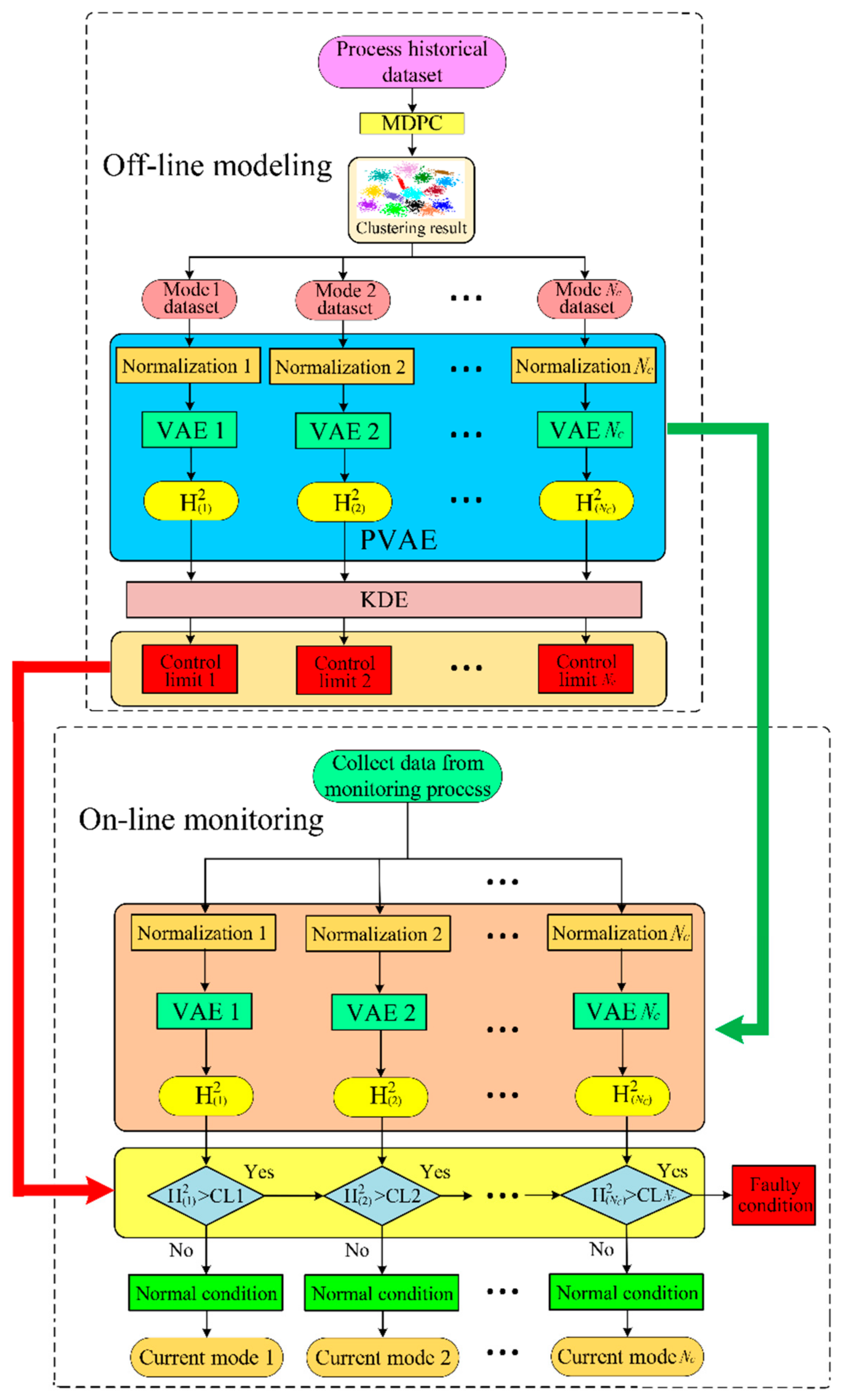
The procedure of MDPC-PVAE based multimode process monitoring is presented in Figure 6. It includes two phases: off-line modeling and on-line monitoring.

Off-line modeling

• Collect the multimode normal process data X and normalize the samples.
• Divide X into $N_c$ data subset $X_1, X_2,\dots , X_{N_c}$ using MDPC.
• Normalize the samples in the data subset and save the normalization parameters for on-line monitoring.
• Design the architecture of PVAE and train the PVAE with data subset $X_1, X_2,\dots , X_{N_c}$.
• Compute the hidden features and construct the monitoring statistic $H_{\left(i\right)}^2$.
• Calculate the control limit with a confidence level of 0.99 for each mode by KDE.

On-line monitoring

• Obtain the on-line sample $x_{new}$ and normalize it by the saved normalization parameters in off-line modeling as $x_{new}^{\left(1\right)}, x_{new}^{\left(2\right)}, \dots , x_{new}^{\left(N_c\right)}$.
• Map $x_{new}^{\left(1\right)}, x_{new}^{\left(2\right)}, \dots , x_{new}^{\left(N_c\right)}$ to the PVAE and obtain the hidden features.
• Calculate statistics $H_{\left(i\right)}^2$; if each statistic is greater than its corresponding control limit $H_{\left(i, lim\right)}^2$, $x_{new}$ is faulty. Otherwise, $x_{new}$ is normal and record the current mode type.

4. Case Study

In this section, two benchmark cases (i.e., TE process and SE process) were conducted to test the monitoring performance of MDPC-PVAE. Based on the requirements of environment and different products, there are various operation conditions in TE process and SE process. They are typical multimode processes that were extensively applied to the performance evaluation of multimode fault detection methods. The simulations were implemented on a computer with configurations as follows: Operating system: 64-bit Microsoft Windows 10; CPU: Intel i7-8700 (3.20 GHz); RAM: 8GB; Software: Matlab2020.

4.1. Tennessee Eastman Process

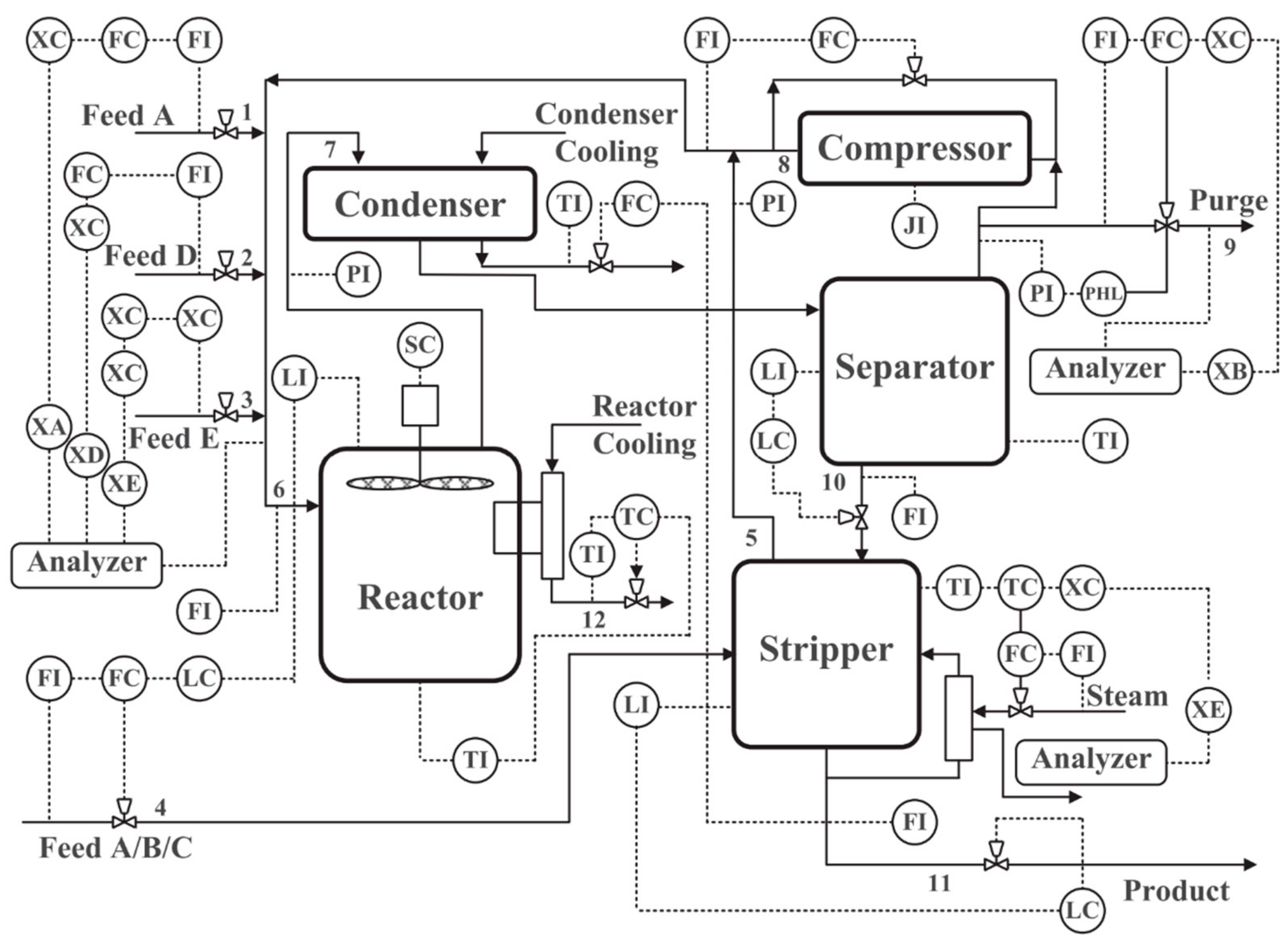
The TE process is a realistic simulation program of a large-scale chemical industrial plan, which has become a benchmark platform for FDD methods evaluation [35]. This process includes five units: the reactor, vapor–liquid separator, product condenser, recycle compressor, and product stripper. There are total of 22 continuous measurement variables, 19 composition measurement variables, and 12 manipulated variables. The flow sheet of TE process is exhibited in Figure 7. In this study, we used the revised TE simulation proposed in [36]. There are six different process operation modes. In each mode, the simulation data include 1 normal dataset and 28 faulty datasets.

Table 1. Description of faults in the TE process.

Fault	Description	Type
1	A/C feed ratio, B composition constant (stream 4)	Step
2	B composition, A/C ratio constant (stream 4)	Step
3	D feed temperature (stream 2)	Step
4	Water inlet temperature for reactor cooling	Step
5	Water inlet temperature for condenser cooling	Step
6	A feed loss (stream 1)	Step
7	C header pressure loss (stream 4)	Step
8	A/B/C composition of stream 4	Random variation
9	D feed (stream 2) temperature	Random variation
10	C feed (stream 4) temperature	Random variation
11	Cooling water inlet temperature of reactor	Random variation
12	Cooling water inlet temperature of separator	Random variation
13	Reaction kinetics	Random variation
14	Cooling water outlet valve of reactor	Sticking
15	Cooling water outlet valve of separator	Sticking
16	Variation coefficient of the steam supply of the heat exchange of the stripper	Random variation
17	Variation coefficient of heat transfer in reactor	Random variation
18	Variation coefficient of heat transfer in condenser	Random variation
19	Unknown	Unknown
20	Unknown	Random variation
21	A feed (stream 1) temperature	Random variation
22	E feed (stream 3) temperature	Random variation
23	A feed flow (stream 1)	Random variation
24	D feed flow (stream 2)	Random variation
25	E feed flow (stream 3)	Random variation
26	A and C feed flow (stream 4)	Random variation
27	Reactor cooling water flow	Random variation
28	Condenser cooling water flow	Random variation

lists the description of these 28 faults. Each dataset is simulated for a duration of 100 h at a sampling rate of 3 min, resulting in 2000 observed samples. In the fault datasets, the abnormal conditions are introduced from the 601st to the 2000th sample.

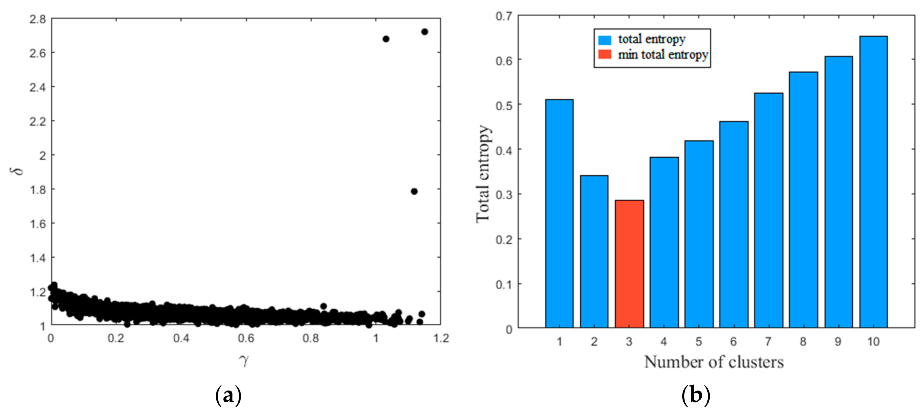
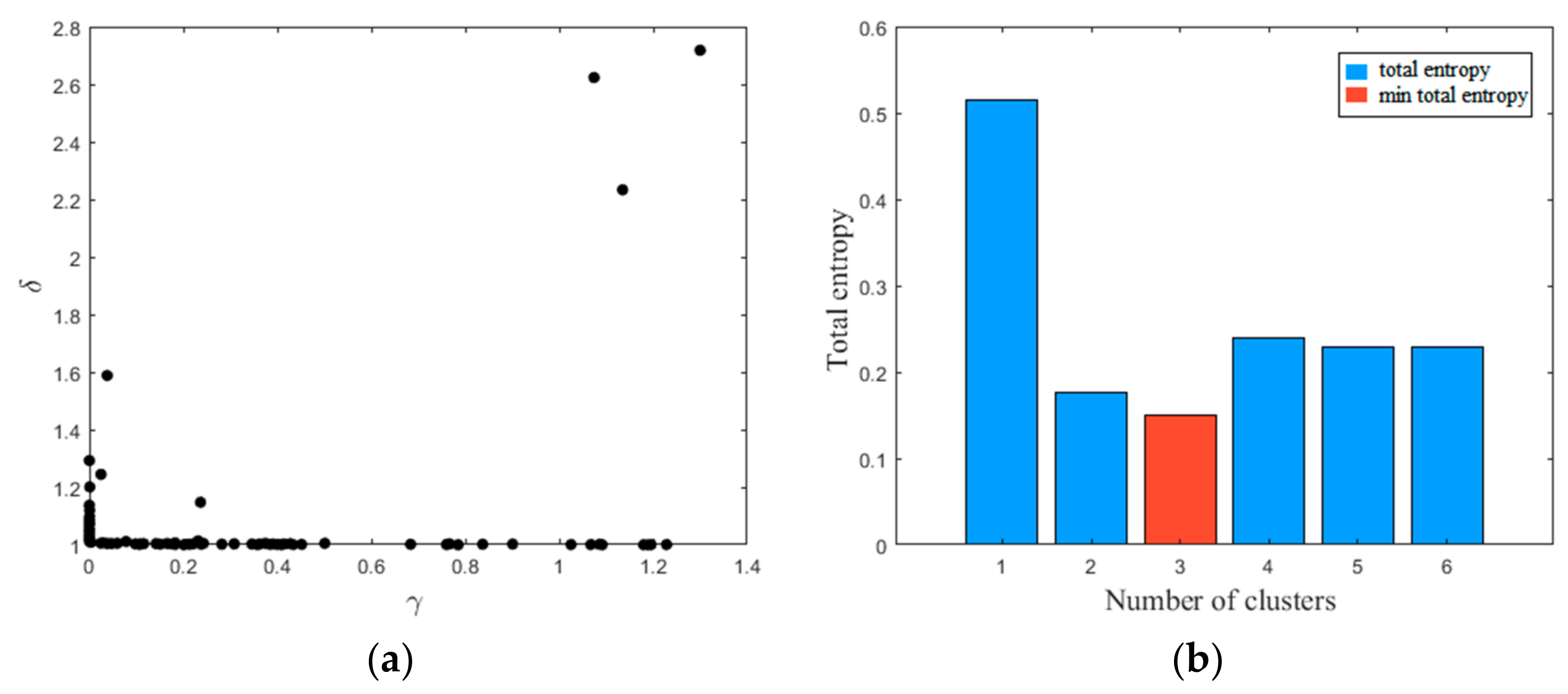
In this study, the operating Modes 1, 2, and 3 were chosen for multimode process simulation. Thirty-three process-measured variables were selected for fault detection modeling. The detail description can be found in [37]. The faults were selected based on different types, including step faults (1, 2, 4–7), random variation faults (8, 10–13, 17, 18, 20, 24–28), sticking fault (14), and unknown faults (19). The three datasets in normal condition are used for clustering analysis and network training. The $\gamma -\delta$ decision graph and total entropy with different number of clusters are shown in Figure 8. The number of clusters was calculated as three. The network parameters and hyperparameters were determined properly by using grid searching. The network structures of PVAE were designed at 33-100-70, 33-95-70, and 33-100-65.

In this case study, three methods including LNS-PCA, MD-kNN, and GMM-SDAE were constructed to compare with the MDPC-PVAE to verify the effectiveness of the proposed method. The number of principal components for LNS-PCA is 17 [38]. The number of neighbors in LNS-PCA and MD-kNN is set to five. The number of multimode parameters in GMM-SDAE is three. The network structures of GMM-SDAE are the same with PVAE. The confidence level of the control limits is 0.99.

In the LNS-PCA and GMM-SDAE, two statistics, i.e., Hotelling’s T-squared ($T^2$) and squared prediction error (SPE), were calculated to detect process faults. The $T^2$ statistic and SPE statistic measure the variation of sample $x_i$ projected in the feature space (h) and residual space ($x-\widehat{x}$), respectively [13,25]. The $T^2$ and SPE statistics are defined as follows:

$$T^2=h_i^T{\varphi }^{-1}{h}_i ,$$

(25)

$$SPE=\parallel x_i-{\widehat{x}}_i{\parallel }^2,$$

(26)

where h is a vector representing the extracted features by LNS-PCA and GMM-SDAE, and $\varphi$ is the covariance matrix. The monitoring statistic $D^2$ of MD-kNN is defined as [39]:

$$D_i^2={\displaystyle \sum }_{j=1}^k{M}_{i,j}^2,$$

(27)

where $M_{i,j}^2$ denotes Mahalanobis distance from sample i to its jth nearest neighbor.

Two important indicators, i.e., fault detection rate (FDR) and false-alarm rate (FAR), were taken for performance evaluation of MDPC-PVAE. They are defined as follows:

$$FDR=\frac{Number of alarms}{Number of faulty samples}\times 100\%,$$

(28)

$$FAR=\frac{Number of false alarms}{Number of normal samples}\times 100\%$$

(29)

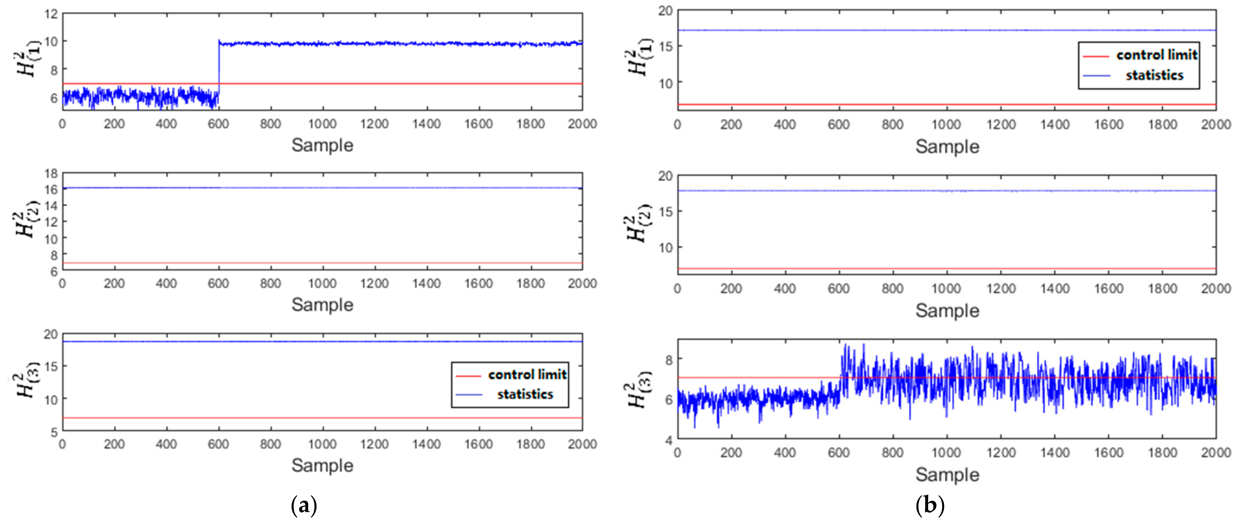
Figure 9 shows the monitoring charts of MDPC-PVAE in the TE process. As shown in Figure 9a, the testing dataset is Fault 4 in Mode 1. The first 600 samples of $H_{\left(1\right)}^2$ are all below its control limit. When the fault occurs at the 601st sample, $H_{\left(1\right)}^2$ begins to increase and exceed the control limit. $H_{\left(2\right)}^2$ and $H_{\left(3\right)}^2$ are always above their control limits. Similarity, in Figure 9b, the $H_{\left(3\right)}^2$ can also recognize the normal samples, and the other two statistics are above the control limits. This is because, due to the generated hidden features from PVAE following the Gaussian distribution, each sub-VAE in the PVAE only recognize the within-mode normal condition. When detecting the faulty condition within-mode or the arbitrary condition in the other modes, the corresponding statistic will be greater than its control limit.

In this case study, a testing dataset for one fault type is composed of the corresponding datasets in three modes. The comparison results of FAR/FDR are exhibited in

Table 2. FAR/FDR of MDPC-PVAE and the other methods on the TE process.

Fault	LNS-PCA		MD-kNN	GMM-SDAE		MDPC-PVAE
	${\mathit{T}}^2$	SPE	${\mathit{D}}^2$	${\mathit{T}}^2$	SPE	${\mathit{H}}^2$
1	3.67/99.86	3.39/99.86	0.89/99.88	2.67/99.81	2.5/99.71	0.67/99.88
2	3.28/99.36	1.56/98.81	0.94/99.29	2.11/99.24	4.17/98.64	0.22/99.26
4	4.33/99.93	2.39/99.93	0.89/99.93	2.83/99.86	2.08/99.86	0.33/99.93
5	5.83/34.96	2.89/34.1	1.61/33.45	4.89/35.12	5.42/33.62	2.33/33.69
6	2.67/100	2.22/100	0.67/100	1.67/99.93	1.46/99.93	0.06/100
7	3.72/99.93	3.06/99.93	1.28/99.93	3/99.86	3.75/99.86	0.39/99.93
8	4.39/99.26	3.06/98.17	1.22/99.21	4.61/99.19	2.5/98.86	1.28/99.24
10	3.78/79.14	2/91.93	0.67/93.09	3/92.88	3.33/92.43	0.28/93.1
11	4.67/98.02	5.11/97.71	0.72/98.21	4.95/98.69	4.38/93.69	1.11/97.93
12	3.89/59.55	2.39/49.74	0.94/55.48	2.55/65.48	2.71/48.24	0.61/64.27
13	6.06/96.07	3.33/95.93	1.67/96.83	6.22/96.83	3.13/92.74	1.94/96.57
14	3.78/97.83	3.33/97.86	1.17/98.62	3.17/98.55	3.13/94.4	0.78/98.31
17	3/91.45	3/94	0.94/93.1	2.72/94.52	1.04/90.24	0.56/93.43
18	5.56/80.02	1.22/82.17	0.67/83.6	4.11/85.6	1.25/78.93	1.11/83.21
19	3.33/98.43	3.06/98.81	1.44/99.02	2.11/99	1.46/98.12	0.28/98.93
20	6.83/97.57	6.78/98.5	1.06/98.31	8.05/98.31	3.75/96.95	2.67/98.33
24	4.5/68.36	4.39/83.88	0.89/87.62	5.39/73.55	3.13/88.52	1.06/88.71
25	3.67/60.64	3.94/68.71	0.33/82	4.11/66.05	2.29/64.19	0.89/73.05
26	4.11/67.55	4.06/86.38	1.5/82.7	3.17/85.55	3.54/69.36	1.17/85.55
27	3.72/77.05	3.17/78.98	0.72/78.40	2.33/83.05	2.08/50.45	0.5/78.81
28	3.56/21.19	3/22.93	0.33/1.48	4.17/24.31	3.13/16.38	0.72/25.11
FDR	4.21/82.2	3.21/84.68	0.98/84.77	3.71/85.49	2.87/81.2	0.9/86.05

. It is obvious that MDPC-PVAE has a relatively high accuracy for most faults, especially for Faults 12, 24, and 28. Moreover, the MDPC-PVAE has the highest average FDR with 86.05% among all the comparison methods. The average FDRs of LNS-PCA (SPE) and GMM-SDAE ($T^2$) are relatively high with 84.68% and 85.49%, respectively. However, their average FARs are also much higher with over 3%. MDPC-PVAE obtains the lowest FAR with 0.9%

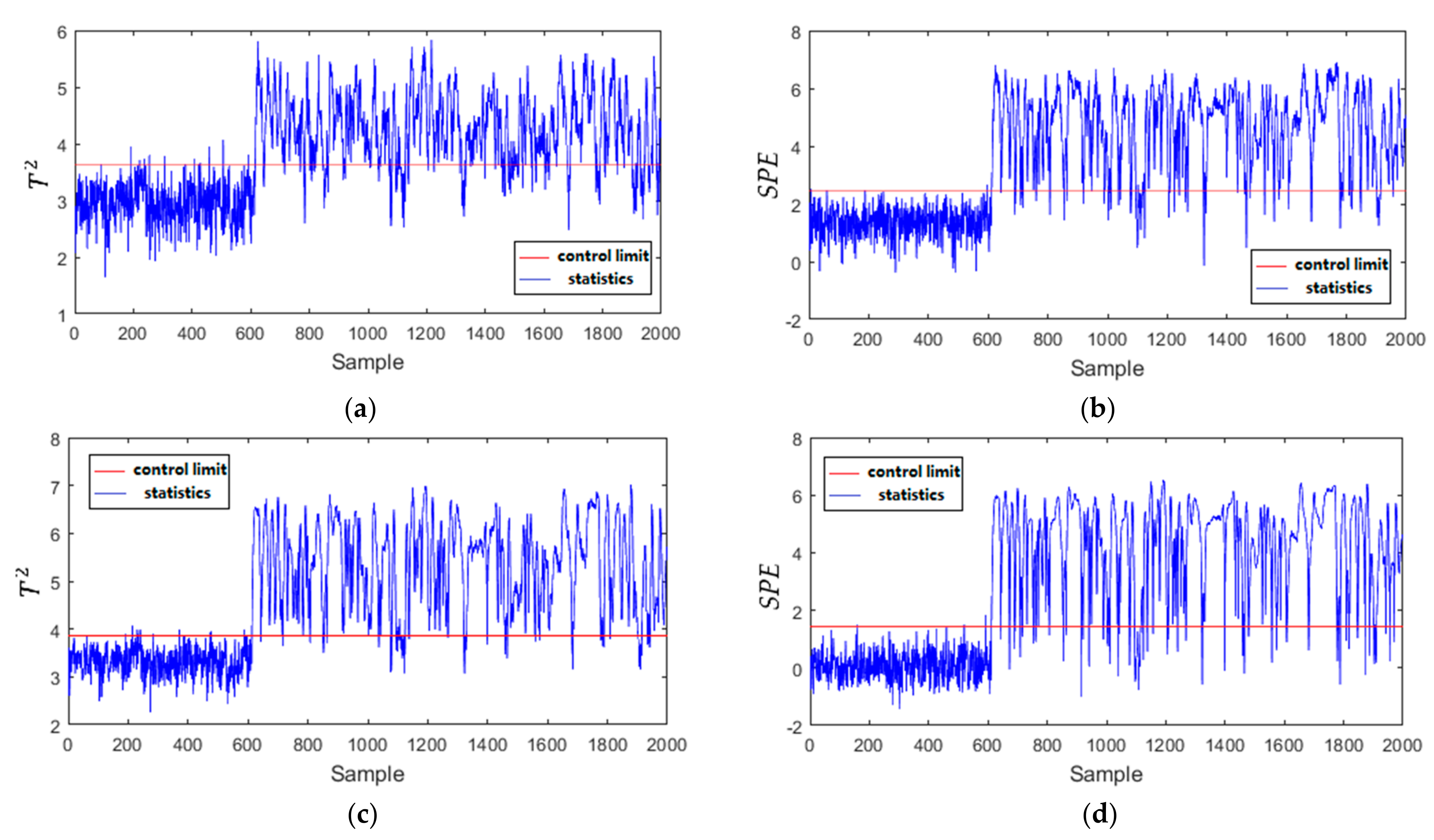
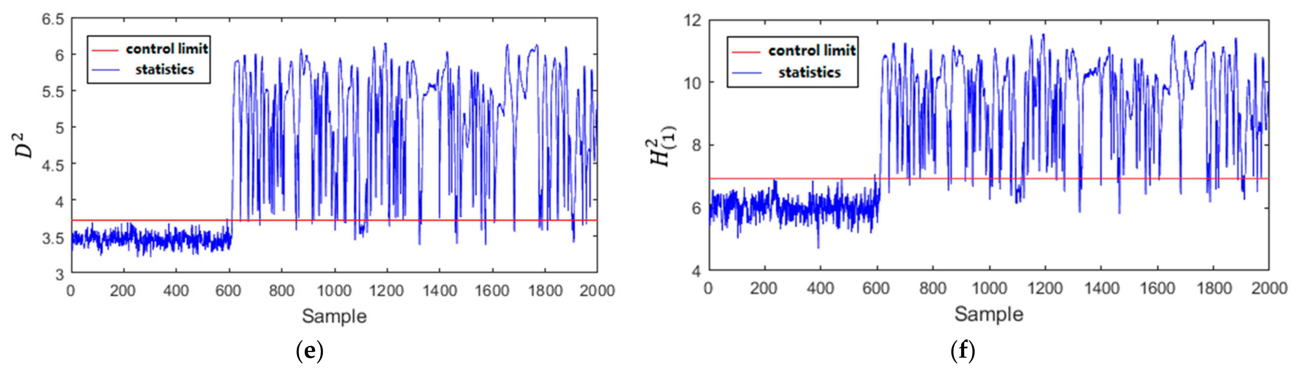
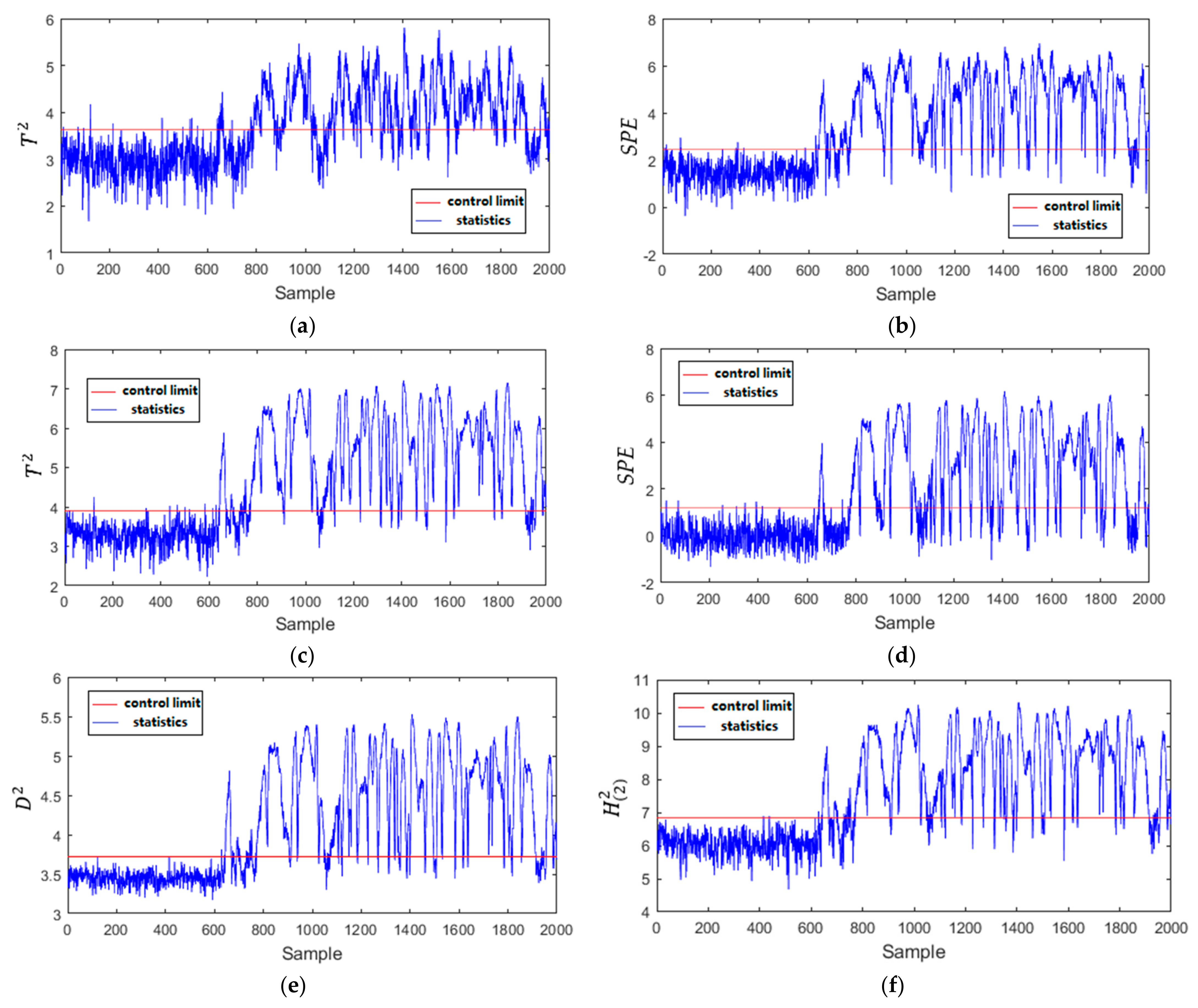
The monitoring results of Fault 25 in Mode 1 with the four methods are shown in Figure 10. The LNS-PCA ($T^2$) only achieves the FDR with 82.14%. LNS-PCA (SPE) and GMM-SDAE ($T^2$ and SPE) can achieve the FDR with about 92%. Furthermore, the LNS-PCA ($T^2$) and GMM-SDAE ($T^2$ and SPE) have higher FAR, about 2%. The performance of the proposed MDPC-PVAE is slightly better than other methods, with an FDR of 94% and FAR of 0.17%. Figure 11 shows the monitoring results of Fault 26 in Mode 2. The LNS-PCA ($T^2$) and GMM-SDAE (SPE) have lower FDRs with 68.71% and 69.71%, respectively. The FDRs of LNS-PCA (SPE) and GMM-SDAE ($T^2$) are relatively high with 86.79% and 84.64%, while their FARs are also correspondingly high with about 1.6%. MD-kNN achieves the FAR of 0%, but its FAR is also low with 82.71%. The FDR and FAR of MDPC-PVAE are 84.14% and 0.33%. MDPC-PVAE has higher FDR and lower FAR. This is because the generated features by MDPC-SAE follow Gaussian distribution, which are more beneficial for statistic construction and fault detection. Compared with the other methods, the proposed MDPC-PVAE can more effectively capture features from the local process data, which improves its performance of multimode fault detection.

The computational complexity of the model is an important evaluation indicator in practical engineering applications. The computational times for the four methods are presented in

Table 3. Testing time of 2000 sample for the four methods.

Method	LNS-PCA	MD-kNN	GMM-SDAE	MDPC-PVAE
Testing time (ms)	67,982.97	72,103.54	347.34	40.51

. The testing time for a batch size is 2000 samples. MDPC-PVAE consumes 40.51 ms. LNS-PCA and MD-kNN consume more time with 67,982.97 and 72,103.54, respectively. This is not a surprise because they both need to search through the whole dataset to find the nearest neighbors, which greatly increases the computational time of the monitoring process. Compared with parallel network structure of MDPC-PVAE, GMM-SDAE only uses a feature extraction network for on-line monitoring. However, the mode of the monitoring sample should be firstly determined by GMM. Meanwhile, in order to obtain the reconstruction error, the decoder network is also used for computing the reconstruction sample. That means the number of hidden layers required for calculating is twice that of MDPC-PVAE, which brings more parameters and more computational burden. Both of the two factors can lead to the increase of testing time.

4.2. Semiconductor Etching Process

The semiconductor dataset was collected from an A1 stack etch process performed on a commercial scale LAM 9600 plasma etch tool at Texas Instrument, Dallas, USA [39,40]. The data consist of 108 normal wafers taken during three experiments and 21 wafers with intentionally induced faults taken during the same experiments. There are 21 variables in a wafer. Excluding the time and step number variables, we selected 19 variables for fault detection modeling. Due to the fact that the original data in the semiconductor etching process are three-dimensional, statistics pattern analysis (SPA) method was adopted to replace the batch data with statistical characteristics of variables. The mean and variance of variables were chosen to constitute the statistics pattern vector of batch.

The $\gamma -\delta$ decision graph and total entropy with different number of clusters are shown in Figure 12. The number of clusters was calculated as three. The network structures of PVAE were designed at 38-50-30, 38-55-30, and 38-55-35. The number of principal components for LNS-PCA is 20. The number of neighbors in LNS-PCA and MD-kNN was set to five. The number of multimode parameters in GMM-SDAE is three.

The detection results of the 21 faults by the four methods are exhibited in

Table 4. Fault detection result of MDPC-PVAE and the other methods in the SE process.

Fault	LNS-PCA		MD-kNN	GMM-SDAE		MDPC-PVAE
	${\mathit{T}}^2$	SPE	${\mathit{D}}^2$	${\mathit{T}}^2$	SPE	${\mathit{H}}^2$
1	√	√	√	√		√
2	√	√	√	√		√
3		√	√			√
4	√	√	√	√	√	√
5	√	√	√	√		√
6		√	√	√		√
7	√	√	√	√	√	√
8	√			√		√
9		√	√	√		√
10		√	√			√
11	√	√	√	√		√
12	√	√	√	√	√	√
13	√	√	√	√	√	√
14	√	√	√	√	√	√
15	√	√	√	√		√
16	√	√	√	√		√
17			√			√
18	√	√	√	√		√
19	√	√	√	√		√
20	√	√	√	√		√
21	√	√	√	√		√
FDR	76.19%	90.48%	95.24%	85.71%	23.81%	100%

. The checkmark represents that the fault is detected by the corresponding method. In LNS-PCA and GMM-SDAE, Faults 3 and 17 are not detected. The SPE statistic of GMM-SDAE only recognizes five faults. LNS-PCA (SPE) and GMM-SDAE (SPE) cannot detect Fault 8. MD-kNN shows good performance in which only Fault 8 is not detected. LNS-PCA ($T^2$) and GMM-SDAE cannot detect Fault 10. Fault 17 is only detected by MD-kNN and MDPC-PVAE. The FDRs of LNS-PCA (SPE), MD-kNN, and GMM-SDAE ($T^2$) are all above 85%. Compared with the other methods, the proposed MDPC-PVAE has a significant performance improvement in the detection of Faults 3, 8, 10, and 17. The result illustrates that MDPC-PVAE has superior performance in multimode fault detection.

5. Conclusions

In this study, the modified density peak clustering and parallel variational autoencoder-based multimode process monitoring method is proposed. The MDPC can identify the number of modes and divide the process data without prior knowledge about mode information. The PVAE is built up based on the divided multimode process data. The Gaussian distribution characteristic of generated features from PVAE is beneficial for improving the fault detection effect and reducing the false alarm. The MDPC-PVAE can solve the inaccurate mode identification problem and the uncertainty of generated features distribution. The effectiveness of the proposed method is verified in the TE process and the SE process. Compared with related multimode process monitoring methods, such as LNS-PCA, MD-kNN, and GMM-SDAE, the simulation results indicate that the MDPC-VPAE has an excellent monitoring performance with the FDRs of 86.05% and 100%, respectively. Furthermore, the testing times show that the MDPC-VPAE has good performance in computational efficiency. It is suitable for real-time monitoring and fault detection in practical engineering applications.

In the on-line monitoring, MDPC-PVAE can directly feed the monitoring data into the generation network without the mode identification phase to detect faults, while the mode information of the faulty data cannot be obtained. In addition, this work mainly studies on the steady modes in multimode process. The transition modes are not explicitly considered. The further investigation is needed for extending this method to monitor transition processes.

References

- Ge, Z.; Song, Z.; Gao, F. Review of Recent Research on Data-Based Process Monitoring. Ind. Eng. Chem. Res. 2013, 52, 3543–3562. [Google Scholar] [CrossRef]
- Montazeri, A.; Ansarizadeh, M.H.; Arefi, M.M. A Data-Driven Statistical Approach for Monitoring and Analysis of Large Industrial Processes. IFAC-PapersOnLine 2019, 52, 2354–2359. [Google Scholar] [CrossRef]
- Qin, S.J. Survey on Data-Driven Industrial Process Monitoring and Diagnosis. Annu. Rev. Control 2012, 36, 220–234. [Google Scholar] [CrossRef]
- Li, Y.; Yang, D. Local Component Based Principal Component Analysis Model for Multimode Process Monitoring. Chin. J. Chem. Eng. 2021, 34, 116–124. [Google Scholar] [CrossRef]
- Tao, Y.; Shi, H.; Song, B.; Tan, S. A Novel Dynamic Weight Principal Component Analysis Method and Hierarchical Monitoring Strategy for Process Fault Detection and Diagnosis. IEEE Trans. Ind. Electron. 2020, 67, 7994–8004. [Google Scholar] [CrossRef]
- Liu, Y.; Pan, Y.; Sun, Z.; Huang, D. Statistical Monitoring of Wastewater Treatment Plants Using Variational Bayesian PCA. Ind. Eng. Chem. Res. 2014, 53, 3272–3282. [Google Scholar] [CrossRef]
- Zhang, Y.W.; Zhou, H.; Qin, S.J. Decentralized Fault Diagnosis of Large-Scale Processes Using Multiblock Kernel Principal Component Analysis. Zidonghua Xuebao/Acta Autom. Sin. 2010, 36, 593–597. [Google Scholar] [CrossRef]
- Chang, Y.; Ma, R.; Zhao, L.; Wang, F.; Wang, S. Online Operating Performance Evaluation for the Plant-Wide Industrial Process Based on a Three-Level and Multi-Block Method. Can. J. Chem. Eng. 2019, 97, 1371–1385. [Google Scholar] [CrossRef]
- Peng, K.; Zhang, K.; You, B.; Dong, J. Quality-Related Prediction and Monitoring of Multi-Mode Processes Using Multiple PLS with Application to an Industrial Hot Strip Mill. Neurocomputing 2015, 168, 1094–1103. [Google Scholar] [CrossRef]
- Li, Z.; Yan, X. Ensemble Learning Model Based on Selected Diverse Principal Component Analysis Models for Process Monitoring. J. Chemom. 2018, 32, e3010. [Google Scholar] [CrossRef]
- Ge, Z.; Song, Z. Online Monitoring of Nonlinear Multiple Mode Processes Based on Adaptive Local Model Approach. Control Eng. Pract. 2008, 16, 1427–1437. [Google Scholar] [CrossRef]
- Song, B.; Shi, H. Temporal-Spatial Global Locality Projections for Multimode Process Monitoring. IEEE Access 2018, 6, 9740–9749. [Google Scholar] [CrossRef]
- Ma, H.; Hu, Y.; Shi, H. A Novel Local Neighborhood Standardization Strategy and Its Application in Fault Detection of Multimode Processes. Chemom. Intell. Lab. Syst. 2012, 118, 287–300. [Google Scholar] [CrossRef]
- Verdier, G.; Ferreira, A. Adaptive Mahalanobis Distance and K-Nearest Neighbor Rule for Fault Detection in Semiconductor Manufacturing. IEEE Trans. Semicond. Manuf. 2011, 24, 59–68. [Google Scholar] [CrossRef]
- Deng, X.; Tian, X. Multimode Process Fault Detection Using Local Neighborhood Similarity Analysis. Chin. J. Chem. Eng. 2014, 22, 1260–1267. [Google Scholar] [CrossRef]
- Yu, J.; Qin, S.J. Multimode Process Monitoring with Bayesian Inference-based Finite Gaussian Mixture Models. AIChE J. 2008, 54, 1811–1829. [Google Scholar] [CrossRef]
- Xie, X.; Shi, H. Dynamic Multimode Process Modeling and Monitoring Using Adaptive Gaussian Mixture Models. Ind. Eng. Chem. Res. 2012, 51, 5497–5505. [Google Scholar] [CrossRef]
- Zhang, S.; Wang, F.; Tan, S.; Wang, S.; Chang, Y. Novel Monitoring Strategy Combining the Advantages of the Multiple Modeling Strategy and Gaussian Mixture Model for Multimode Processes. Ind. Eng. Chem. Res. 2015, 54, 11866–11880. [Google Scholar] [CrossRef]
- Ben Khediri, I.; Weihs, C.; Limam, M. Kernel K-Means Clustering Based Local Support Vector Domain Description Fault Detection of Multimodal Processes. Expert Syst. Appl. 2012, 39, 2166–2171. [Google Scholar] [CrossRef]
- Ge, Z.; Song, Z. Multimode Process Monitoring Based on Bayesian Method. J. Chemom. 2009, 23, 636–650. [Google Scholar] [CrossRef]
- Xie, X.; Shi, H. Multimode Process Monitoring Based on Fuzzy C-Means in Locality Preserving Projection Subspace. Chin. J. Chem. Eng. 2012, 20, 1174–1179. [Google Scholar] [CrossRef]
- Luo, L.; Bao, S.; Mao, J.; Tang, D. Phase Partition and Phase-Based Process Monitoring Methods for Multiphase Batch Processes with Uneven Durations. Ind. Eng. Chem. Res. 2016, 55, 2035–2048. [Google Scholar] [CrossRef]
- Quiñones-Grueiro, M.; Prieto-Moreno, A.; Verde, C.; Llanes-Santiago, O. Data-Driven Monitoring of Multimode Continuous Processes: A Review. Chemom. Intell. Lab. Syst. 2019, 189, 56–71. [Google Scholar] [CrossRef]
- Rodriguez, A.; Laio, A. Clustering by Fast Search and Find of Density Peaks. Science. 2014, 344, 1492–1496. [Google Scholar] [CrossRef] [Green Version]
- Li, S.; Zhou, X.; Shi, H.; Pan, F.; Li, X.; Zhang, Y. Multimode Processes Monitoring Based on Hierarchical Mode Division and Subspace Decomposition. Can. J. Chem. Eng. 2018, 96, 2420–2430. [Google Scholar] [CrossRef]
- Zheng, Y.; Wang, Y.; Yan, H.; Wang, Y.; Yang, W.; Tao, B. Density Peaks Clustering-Based Steady/Transition Mode Identification and Monitoring of Multimode Processes. Can. J. Chem. Eng. 2020, 98, 2137–2149. [Google Scholar] [CrossRef]
- Xu, X.; Xu, D.; Wang, X. Anomaly Detection with GRU Based Bi-Autoencoder for Industrial Mul- Timode Process. Int. J. Control. Autom. Syst. 2022, 20, 1827–1840. [Google Scholar] [CrossRef]
- Gao, H.; Wei, C.; Huang, W.; Gao, X. Multimode Process Monitoring Based on Hierarchical Mode Identification and Stacked Denoising Autoencoder. Chem. Eng. Sci. 2022, 253, 117556. [Google Scholar] [CrossRef]
- Zhang, Z.; Jiang, T.; Zhan, C.; Yang, Y. Gaussian Feature Learning Based on Variational Autoencoder for Improving Nonlinear Process Monitoring. J. Process Control 2019, 75, 136–155. [Google Scholar] [CrossRef]
- Tang, P.; Peng, K.; Jiao, R. A Process Monitoring and Fault Isolation Framework Based on Variational Autoencoders and Branch and Bound Method. J. Franklin Inst. 2022, 359, 1667–1691. [Google Scholar] [CrossRef]
- Guo, F.; Wei, B.; Huang, B. A Just-in-Time Modeling Approach for Multimode Soft Sensor Based on Gaussian Mixture Variational Autoencoder. Comput. Chem. Eng. 2021, 146, 107230. [Google Scholar] [CrossRef]
- Xu, J.; Cai, Z. Gaussian Mixture Deep Dynamic Latent Variable Model with Application to Soft Sensing for Multimode Industrial Processes. Appl. Soft Comput. 2022, 114, 108092. [Google Scholar] [CrossRef]
- Li, M.; Bi, X.; Wang, L.; Han, X. A Method of Two-Stage Clustering Learning Based on Improved DBSCAN and Density Peak Algorithm. Comput. Commun. 2021, 167, 75–84. [Google Scholar] [CrossRef]
- Li, J.; Yan, X. Process Monitoring Using Principal Component Analysis and Stacked Autoencoder for Linear and Nonlinear Coexisting Industrial Processes. J. Taiwan Inst. Chem. Eng. 2020, 112, 322–329. [Google Scholar] [CrossRef]
- Bathelt, A.; Ricker, N.L.; Jelali, M. Revision of the Tennessee Eastman Process Model. IFAC-PapersOnLine 2015, 28, 309–314. [Google Scholar] [CrossRef]
- Reinartz, C.; Kulahci, M.; Ravn, O. An Extended Tennessee Eastman Simulation Dataset for Fault-Detection and Decision Support Systems. Comput. Chem. Eng. 2021, 149, 107281. [Google Scholar] [CrossRef]
- Jiang, L.; Ge, Z.; Song, Z. Semi-Supervised Fault Classification Based on Dynamic Sparse Stacked Auto-Encoders Model. Chemom. Intell. Lab. Syst. 2017, 168, 72–83. [Google Scholar] [CrossRef]
- Guo, Q.; Liu, J.; Tan, S. A multimode process monitoring strategy via improved variational inference Gaussian mixture model based on locality preserving projections. Trans. Inst. Meas. Control 2022, 44, 1732–1743. [Google Scholar] [CrossRef]
- He, Q.P.; Wang, J. Fault Detection Using the K-Nearest Neighbor Rule for Semiconductor Manufacturing Processes. IEEE Trans. Semicond. Manuf. 2007, 20, 345–354. [Google Scholar] [CrossRef]
- Zhang, C.; Gao, X.; Li, Y.; Feng, L. Fault Detection Strategy Based on Weighted Distance of k Nearest Neighbors for Semiconductor Manufacturing Processes. IEEE Trans. Semicond. Manuf. 2019, 32, 75–81. [Google Scholar] [CrossRef]
Figure 1.
The basic structure of VAE.
Figure 2.
MDPC on the Aggregation dataset: (a) decision graph; (b) total entropy with different number of clusters; (c) visual clustering result.
Figure 3.
MDPC on the R15 dataset: (a) decision graph; (b) total entropy with different number of clusters; (c) visual clustering result.
Figure 4.
MDPC on the D31 dataset: (a) decision graph; (b) total entropy with different number of clusters; (c) visual clustering result.
Figure 5.
Comparison of clustering results on the Aggregation dataset: (a) DPC; (b) DBSCAN; (c) MDPC.