The Effects of Cognitive and Skill Learning on the Joint Vendor–Buyer Model with Imperfect Quality and Fuzzy Random Demand

Abstract

This study investigates the optimization of an integrated production–inventory system that consists of an original equipment manufacturer (OEM) supplier and an OEM brand company. The cognitive and skill learning effect, imperfect quality, and fuzzy random demand are incorporated into the integrated two-echelon supply chain model to minimize the total cost. We contribute to dividing the learning effect into cognitive learning and skill learning, we build a new learning curve to resemble the real complexity more closely and avoid the problem that production time tends towards zero after production is stable. In total, five production–inventory models are constructed. Furthermore, a solution procedure is designed to solve the model to obtain the optimal order quantities, and the optimal shipment size. Additionally, the symbolic distance method is used to deal with the inverse fuzzification. Then numerical analysis shows that the increase of the cognitive learning coefficient and skill learning coefficient will reduce the total cost of the production–inventory system. With the increase of the cognitive learning coefficient, the gap between the total cost of cognitive learning and skill learning, and that of Wright learning, correspondingly decreases consistently. However, with the increase of the skill learning coefficient, there is a consistent corresponding increase. The total cost of cognitive learning and skill learning shows hyperbolic characteristics. The important insights of this study for managers are that employees’ knowledge plays an important role in reducing costs in the early learning stage and humanistic management measures should be taken to reduce employees’ turnover. Compared with the skill learning training for production technicians, we should pay more attention to the training of cognitive learning.

1. Introduction

In labor-intensive manufacturing enterprises, when employees carry out repetitive labor, the time to complete one unit will decrease with each iteration, which indirectly leads to the lowering of production cost per unit. This kind of phenomenon is called the learning phenomenon or learning effect. Studying the impact of employees’ learning behavior can better establish an incentive system and reduce the turnover rate of front-line core employees, to reduce the production cost of manufacturing enterprises. Employee learning can improve production efficiency and reduce production costs, but with the increase of productivity, inventory accumulation is accelerated, and inventory costs are increased. It is necessary to balance storage and production.

Although there are many studies on vendor–buyer in the current literature [1,2,3,4]. Few researchers paid too much attention on the vendor–buyer model with simultaneous consideration of learning effects and fuzzy random demand. In order to make up for the deficiency of the existing research on vendor–buyer model consisting of learning effects and fuzzy random demand, this paper tries to develop an integrated production–inventory model to minimize the average annual cost of an integrated two stage supply chain. Additionally, an algorithm is provided to obtain an optimal production–inventory policy for a single-vendor (the OEM supplier)–single-buyer (the OEM Brand Corporation) system with imperfect products and fuzzy demand.

The research problem of this paper is to give the optimal supply strategy when employees have a learning effect in the JIT production environment, that is, the optimal supply times and single supply quantity. In addition, this paper aims to solve the problem that the production time cannot be zero after the production is stable.

The remainder of this paper is organized as follows: Section 2 is the literature review, Section 3 is the problem description, symbolic description, and model hypothesis. Then, Section 4 covers the production–inventory joint optimization model without learning characteristics, while Section 5 covers the production–inventory joint optimization model under different learning efficiency curves. Section 6 elucidates the solution algorithm of the model, and Section 7 compares the solution results of each model. Finally, Section 8 concludes and summarizes this paper.

2. Literature Review

The literature related to this paper can be divided into three groups, the first group is about the just-in-time (JIT) production–inventory optimization, the second group is about the production–inventory optimization with learning effects, and the third group is about the production–inventory optimization considering imperfect quality.

2.1. Related Works on JIT Production–Inventory Optimization

There is a great deal of extant literature around the just-in-time (JIT) production–inventory systems. JIT is one of the important pillars of the Toyota Production System (TPS), which pursues a policy of zero inventory. Practice has proven that JIT strategy can reduce inventory costs and increase profits. The lot-for-lot policy is a salient feature of JIT strategy. Small lot size production with small lot shipment is used in lot-for-lot policy. Small lot shipments need frequent delivery. Since frequent deliveries can significantly reduce buyer inventory costs, many manufacturers adopt small lot shipment in JIT implementation. It is necessary to balance inventory and delivery costs.

Many researchers have studied the integrated manufacturer retailer inventory model for JIT production and shipment policy. Dmua et al. [1] undertook a systematic review of integrated production–inventory model. Based on resource recycling and emission reduction, Chen and Bidanda [5] took component recovery and emission control into consideration and addressed a new production–inventory problem of multiple factories with the JIT policy. By treating the random demand process as a compound Poisson process, De et al. [6] solved a production–inventory problem in which the production rate can be continuously controlled. Nambiar et al. [7] studied an inventory allocation problem in a two-echelon setting with lost sales. Sepehri et al. [8] elaborated a sustainable production–inventory model for poor quality deteriorating items to help decision makers make more efficient replenishment and pricing decisions.

2.2. Related Works on Production–Inventory Optimization with Learning Effect

The existence of the learning effect makes manufacturing costs decrease, according to certain rules. This provides conditions for enterprises to create additional value. Many scholars introduced the learning effect into the economic production quality (EPQ) model. By accounting for rework time, Jaber and Guiffrida [9] proposed a composite learning curve which comprised two learning curves: one describes the reduction in time for normal operation, while the other describes the reduction in time for reworking production. Jaber et al. [10] extended [11] by assuming the percentage of defective items per lot reduces according to a learning curve. In [9,10,11], the researchers did not take learning effects in the supply chain into consideration, they just considered the learning effect in economic production quantity (EOQ)/(EPQ) models of a single-stage production–inventory system. Some scholars studied the two-stage production–inventory problem by taking learning effects into consideration. Khan et al. [12] took human factors into a two-level supply chain, in which suppliers provided imperfect raw materials to the vendor. Considering the learning effect of employees and the errors in the quality inspection process, Khan et al. [13] expanded the model of Huang [14] and Khan et al. [12] and analyzed the impact of producer risk and consumer risk on the number of supply and single supply.

In the research of production–inventory optimization, there are two methods to deal with the uncertainty of demand. One is to use probability theory and the stochastic process method and the other is to introduce fuzzy concepts. Generally, probability theory and stochastic process methods are used to deal with demand uncertainty in academic circles. However, when the random distribution characteristics of demand are not clear, the processing method of fuzzy mathematics can solve the problem of demand uncertainty more effectively. Based on the partial backlogging of shortage, Mahata [15] investigated the learning effect on optimal lot size for the imperfect production process in fuzzy random environments.

Previously, when studying the learning effect, most scholars neglected the cognitive learning process, or simply mixed cognitive learning with skill learning, which made the learning curve unrealistic. Cognitive learning refers to people’s learning in the cognitive process. Cognitive learning is mainly a process of information exchange. In the process of information exchange, people acquire information through perception, attention, memory, and understanding [16]. Skill learning refers to the individual’s learning in the process of operation. The existence of skill learning results in the operator’s proficiency continuously increasing. Prior to manufacturing, the manufacturer needs to spend a lot of time understanding the structure, composition, and the production process of the product, and then time is spent processing the product after mastering the relevant product knowledge. Therefore, it is of practical significance to consider this cognitive and skill learning effect in the simulation of the learning curve of productivity improvement.

2.3. Related Works on Production–Inventory Optimization with Imperfect Quality

In the actual production process, there is a possibility that the process veers out of control, thus producing imperfect items. Since the imperfectness of production conditions in practice, considering imperfect quality problem in production–inventory optimization, has become an important topic, many authors have conducted research in this area. The imperfection of the actual production process leads to the quality defects of the products. Many scholars pointed out the incomplete characteristics of quality in inventory optimization [17,18,19]. Assuming shortages are allowed, as is price-dependent demand, Khanna et al. [20] developed an inventory model for items of imperfect quality under trade–credit policies. Salas-Navarro et al. [21] proposed an EPQ inventory model considering imperfect items and probabilistic demand for a two-echelon supply chain. They found that the collaborative approach generates greater profits for the supply chain. Sepehri et al. [22] elaborated a sustainable production–inventory model for poor quality deteriorating items to help decision makers make more efficient replenishment and pricing decisions. Kurdhi et al. [23] developed an integrated inventory model considering the imperfect quality items, inspection error, controllable lead time, and budget capacity constraints. Establishing the optimal solution using Kuhn–Tucker’s conditions, they obtained minimum integrated inventory total cost rather than separated inventory. Salameh and Jaber [11] considered the impact of product quality defects when establishing the classical EOQ model. Huang [14] considered the incompleteness in the production process and established a production–inventory joint optimization model with quality defects under the assumption that the quality defects obey uniform distribution. However, Huang [14] did not consider the incompleteness of the quality inspection process itself and the two types of quality inspection risks in the quality inspection process. Hsu and Hsu [23] also considered two types of quality inspection risks in the quality inspection process based on Huang [14]. Hsu and Hsu [24] considered allowing out of stock and completely delaying the supply of out of stock, which was expanded based on Hsu and Hsu [23] models. A comparison between previous studies and this study is shown in

Table 1. Major considerations of the models in the different literature.

	Production–Inventory	Fuzzy Demand	Imperfect Quality	Skill Learning	Cognitive Learning
Chen and Bidanda [5]	Yes	No	No	No	No
Jaber and Guiffrida [9]	No	No	Yes	Yes	No
Jaber et al. [10]	No	No	Yes	Yes	No
Salameh and Jaber [11]	No	No	Yes	Yes	No
Khan et al. [12]	Yes	No	No	Yes	No
Khan et al. [13]	Yes	No	Yes	Yes	No
Huang [14]	Yes	No	Yes	No	No
Mahata [15]	Yes	Yes	Yes	Yes	No
Jaber and Glock [16]	No	No	No	Yes	No
Khanna et al. [20]	Yes	No	Yes	No	No
Hsu and Hsu [23]	Yes	No	Yes	No	No
Dar-el [26]	No	No	No	Yes	Yes
This paper	Yes	Yes	Yes	Yes	Yes

.

The paper establishes five JIT production–inventory joint optimization models, which are based on the learning effect in the process of employees’ work and the uncertain fuzzy demand of retailers due to the product quality defects caused by the incomplete production process. Our models consider no learning effect, instant Wright learning effect, average learning effect, cognitive learning, and skill learning effect. The contribution of this paper is that the learning behavior of employees is divided into cognitive learning and skill learning, and a new learning curve closer to the real complexity is constructed. The new learning curve can avoid the problem that the production time tends towards zero after the production is stable under Wright learning. The FCLCM curve presented in this paper is closer to the complexity of real production. The model built in the paper is based on Huang’s [14] model and Pan and Yang’s [25] method. The difference between Model 1 and Huang’s [14] is that the fuzzy demand is considered; Model 2 and Khan’s [13] are different because the fuzzy demand is considered; Model 3 is based on the Wright learning curve and on Model 1, where the Wright joint production–inventory optimization model with average productivity is established. Model 4 is based on the JGLCM proposed by Jaber and Glock [16]. On the basis of Model 1, the JGLCM joint production–inventory optimization model is established. Model 5 is based on the FCLCM curve proposed by the author and on the basis of Model 1, thus the FCLCM joint production–inventory optimization model is established. The paper enriches the JIT production–inventory literature but also enriches the learning curve theory.

3. Problem Description, Symbol Description, and Model Assumptions

A situation is developed with a two-echelon supply chain system made up of one OEM supplier and one OEM brand under learning effects and fuzzy random demand, in which a lot-for-lot strategy in a production cycle is executed. The OEM Brand Corporation sells a kind of sports shoe, which is limited to its production capacity. After designing a sample of the sports shoe, the OEM Brand Corporation outsources the whole production process of the shoes to a supplier of OEM. OEM suppliers and OEM brand companies constitute a production–inventory system. OEM suppliers need to organize workers to learn about the production process of the sports shoes after receiving orders from OEM brands. Knowledge learning and skill learning are extant in the process of production and manufacturing.

For OEM suppliers, there are many uncertainties in the process of employees’ operation, which leads to the defects of sports shoes. For the OEM brand, it carries out a quality inspection on the sports shoes provided by OEM suppliers every time. The defective products detected are transported back to OEM suppliers for processing, and the qualified products are used for exhibition cabinet sales.

To satisfy the demand for items, the OEM brand purchases items with the order size ($nQ$) from the OEM supplier. The objective of this production–inventory systems is to determine the economic lot size, $Q$, and number of deliveries, $n$, to keep the joint annual cost incurred by the OEM supplier and OEM brand corporation as low as possible.

The establishment of this study’s model is based on the following assumptions:

• The production–inventory system consists of one OEM supplier and one OEM brand. OEM brand company entrusts OEM suppliers to produce a class of sports shoes. Due to the uncertainty in the process of employees’ work, there are quality defects in the sports shoes produced and the defect rate is constant $\gamma$ (%);
• Employees of OEM suppliers have learning behaviors in the process of production and operation. Learning behaviors include cognitive learning and skill learning. Employees’ learning behavior makes productivity change dynamically;
• OEM brand suppliers carry out 100% quality inspection of sports shoes supplied by the OEM suppliers, and the quality inspection process is completed instantaneously. The unit cost of OEM brand suppliers is $\vartheta$ ($/unit). After quality inspection, the number of qualified products available for retail sale by OEM brands is $Q$;
• The demand of OEM brand dealers is a triangular fuzzy number $\tilde{D}$, $\tilde{D}=(D-{\Delta }_1, D, D+{\Delta }_2)$, $0<{\Delta }_1<D$, $0<{\Delta }_2$. $D-{\Delta }_1$ is the lower limit of fuzzy demand, $D$ is the average demand, and $D+{\Delta }_2$ is the upper limit of fuzzy demand. Under the condition of fuzzy demand $\tilde{D}$, the time interval of two consecutive deliveries is $T=Q(1-\gamma )/\tilde{D}$;
• The production–inventory system does not allow an out-of-stock situation, OEM suppliers must have sufficient production capacity to meet the OEM brand order needs, that is, $P>\frac{\tilde{D}}{1-\gamma }$, where $P$ is the OEM supplier staff efficiency, abbreviated as employee productivity;
• OEM brand carries the transportation cost, and the cost of each transportation is fixed.

The parameters and variables used in this model are defined as follows.

Parameters and variables related to the OEM supplier:

• $b$—Learning coefficient under WLC;
• $\phi$—Learning efficiency;
• $b_c$—Cognitive learning coefficient;
• $b_m$—Skills learning coefficient;
• $b^{\ast }$—Compound learning coefficients of employees with cognitive learning and skill learning characteristics;
• $T_1$—The production time required to complete the first pair of sneakers;
• $T_p$—Employees’ working behavior does not have the learning characteristics of one cycle production time;
• $T_d$—Employees’ work behavior does not have one cycle of non-production time under learning characteristics;
• $T_{iQ}$—The time required for the first production of $Q$ pairs of sneakers in the ith cycle with learning characteristics;
• $T_{pi}$—The production time of the ith cycle under the learning characteristics of employees’ work behavior;
• $T_{di}$—The non-production time of the ith cycle under the learning characteristics of employees’ work behavior;
• $\tilde{D}$—The demand;
• $S_v$—Production preparation cost (USD/year);
• $h_v$—Unit time storage cost per unit product (USD/unit/year);
• $v$—Unit defect quality assurance cost (USD/unit);
• $Q$—Quantities of a shipment from the OEM supplier to the OEM brand in a production cycle (a decision variable);
• $n$—The number of shipments from the OEM supplier to the OEM brand in a production lot (a decision variable, a positive integer);
• $Q_p$—$Q_p=nQ$, the lot size in a production cycle.
• $c$—Production cost (USD/year);
• $P$—Employee’s productivity (unit/year) without learning characteristics;
• $\overline{P^w}$—The average productivity of employees with Wright learning characteristics (unit/year);
• $\overline{P^{cm}}$—Employees’ work behavior has the average productivity (unit/year) under the characteristics of knowledge learning and skill learning.

Parameters and variables related to the OEM brand enterprise:

• $S_B$—Ordering fee (RMB/time);
• $F$—Fixed cost per transport (USD/time);
• $\vartheta$—Unit Quality Inspection Cost (USD/time);
• $b_B$—Unit time storage cost per unit product (USD/unit/year).

4. Joint Production–Inventory Optimization without Learning Characteristics for Employees’ Operational Behavior (Model 1)

(1)

OEM supplier cost model

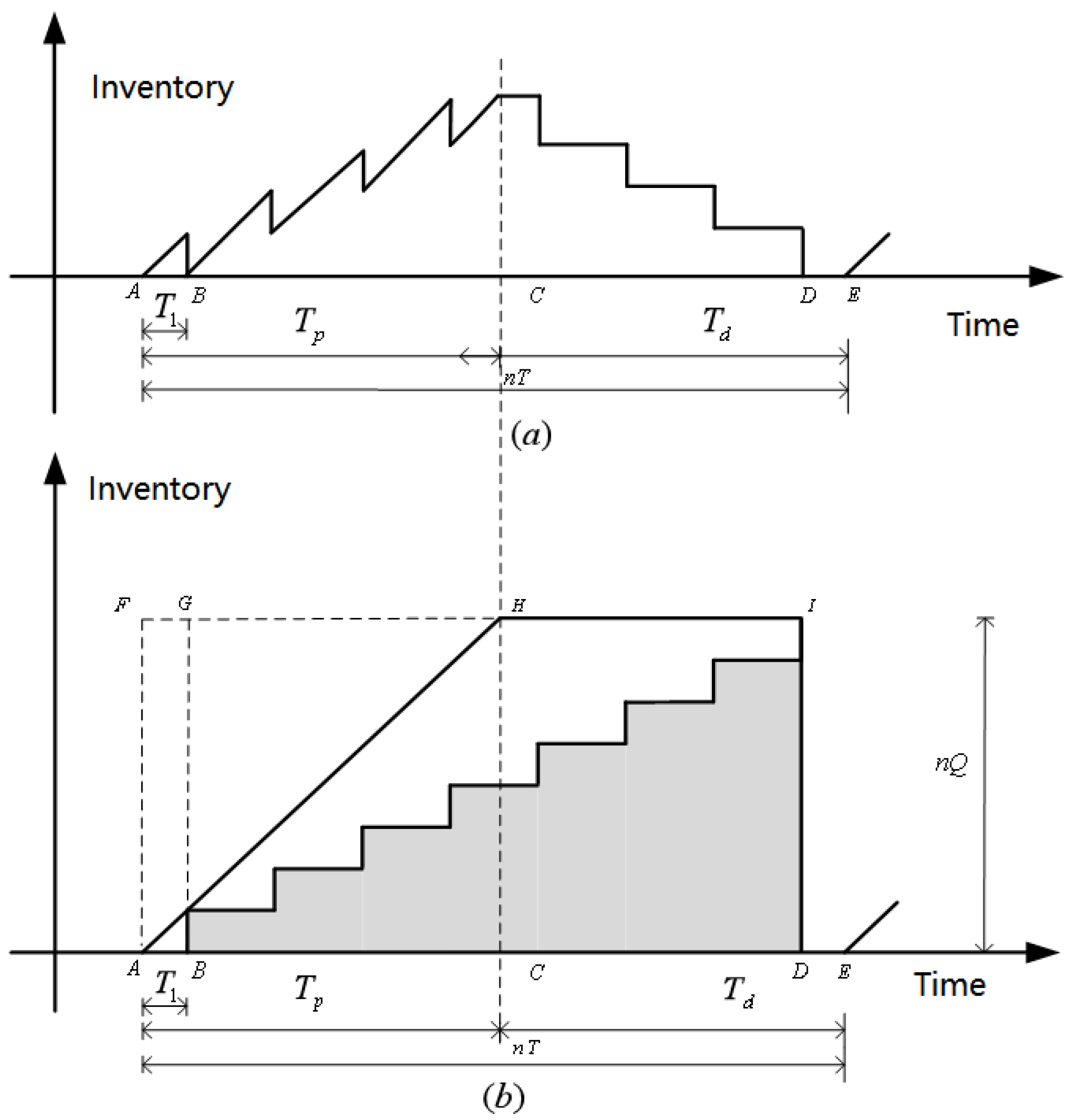
The production–inventory cost model without learning characteristics is the basis of this paper, which provides a reference for the establishment of other models. Figure 1a reflects the actual inventory level of the OEM supplier over time in a production cycle; In Figure 1b, the solid part of the figure shows the cumulative inventory level of OEM suppliers over time when the OEM supplier is not supplying, and the shaded part shows the cumulative inventory of the OEM supplier to the OEM brand enterprise.

Following the method in Khan et al. [13], Huang [14], and Goyal et al. [27], the cost of the OEM supplier and the OEM brand enterprise is calculated. The time of a production cycle includes production time and non-production time. Production time is $T_p=\frac{nQ}{P}$, and non-production time is $T_d=nT-\frac{nQ}{P}$. The length of DE time in Figure 1 is $T-\frac{Q}{P}$, where $T=\frac{(1-\gamma )Q}{\tilde{D}}$. CD duration is $(n-1)\left[\frac{Q(1-\gamma )}{\tilde{D}}-\frac{Q}{P}\right]$. In Figure 1b, the area of triangle ACH is $\frac{n^2{Q}^2}{2P}$, the area of quadrilateral CDHI is $n(n-1)Q^2\left(\frac{1-\gamma }{\tilde{D}}-\frac{1}{P}\right)$, and the area of the shadow part is $\frac{n(n-1)(1-\gamma )Q^2}{2\tilde{D}}$.

The average inventory of the OEM supplier is:

$$\frac{n^2{Q}^2}{2P}+n(n-1)Q^2\left(\frac{1-\gamma }{\tilde{D}}-\frac{1}{P}\right)-\frac{n(n-1)(1-\gamma )Q^2}{2\tilde{D}}.$$

(1)

The total cost of the OEM supplier in a production cycle is the sum of production preparation cost, defective quality assurance cost, production cost, and storage cost.

$$T{C}_v(n,Q)=S_v+vnQ\gamma +c\frac{nQ}{P}+h_v\left[\frac{n^2{Q}^2}{2P}\right.+n(n-1)Q^2\left(\frac{1-\gamma }{\tilde{D}}-\frac{1}{P}\right)-\left.\frac{n(n-1)(1-\gamma )Q^2}{2\tilde{D}}\right].$$

(2)

(2)

The OEM Brand enterprise Cost Model

OEM brand companies use a continuous inventory control strategy to control inventory. Considering the quality defects caused by the uncertainty of employees’ working behavior, the average inventory of the OEM brand after one delivery is $\frac{{(1-\gamma )}^2{Q}^2}{2\tilde{D}}$. In a production cycle, under the condition of the OEM supplier’s $n$ supply times, the total annual cost of the OEM Brand enterprise is as follows:

$$T{C}_B(n,Q)=S_B+nF+\vartheta nQ+\frac{n{h}_B{(1-\gamma )}^2{Q}^2}{2\tilde{D}}.$$

(3)

The first item in Equation (3) is the order cost, the second item is the transportation cost, the third item is the quality inspection cost, and the fourth item is the storage cost.

When the OEM brand enterprise and the OEM supplier form a virtual stakeholder, the virtual stakeholder can make centralized decisions based on the overall interests and make decisions to minimize the cost of the production–inventory system. The total cost of an integrated production–inventory system is:

$$\begin{array}{l}TC(n,Q)=T{C}_v(n,Q)+T{C}_B(n,Q)\\ =S_v+vnQ\gamma +c\frac{nQ}{P}+S_B+nF+\vartheta nQ+\frac{n{h}_B{(1-\gamma )}^2{Q}^2}{2\tilde{D}}\\ +h_v\left[\frac{n^2{Q}^2}{2P}\right.+n(n-1)Q^2\left(\frac{1-\gamma }{\tilde{D}}-\frac{1}{P}\right)-\left.\frac{n(n-1)(1-\gamma )Q^2}{2\tilde{D}}\right]\end{array}.$$

(4)

From Equation (4), the average annual cost of an integrated production–inventory system can be obtained.

$$\begin{array}{l}ATC(n,Q)=\frac{TC(n,Q)}{nT}=\frac{\tilde{D}(S_B+S_v+nF)}{n(1-\gamma )Q}+\frac{\tilde{D}(\vartheta +v\gamma )}{1-\gamma }+\frac{c\tilde{D}}{P(1-\gamma )}\\ +\frac{h_{B}Q(1-\gamma )}{2}+h_{v}Q\left[\frac{2\tilde{D}-n\tilde{D}}{2P(1-\gamma )}+\frac{n-1}{2}\right]\end{array}.$$

(5)

In Equation (5), the average cost of the system is a fuzzy function because the demand is fuzzy. To obtain the optimal number of times and quantity of supply, it is necessary to perform $ATC(n,Q)$ inverse fuzzification. Let $\tilde{U}(n,Q)=ATC(n,Q)$, the symbolic distance method [25] is used to deal with the inverse fuzzification. The symbol distance from $\tilde{U}(n,Q)$ to ${\tilde{0}}_1$ is

$$\begin{array}{ll}\mathrm{d}[\tilde{U}(n,Q),{\tilde{0}}_1]& =\mathrm{d}(\tilde{D},{\tilde{0}}_1)\left[\frac{S_B+S_v+nF}{n(1-\gamma )Q}+\right.\frac{\vartheta +v\gamma }{1-\gamma }+\frac{c}{P(1-\gamma )}+\left.\frac{h_{v}Q(2-n)}{2P(1-\gamma )}\right]\\ & +\frac{h_{B}Q(1-\gamma )}{2}+\frac{h_{v}Q(n-1)}{2}\end{array}.$$

(6)

In Equation (6), $\mathrm{d}(\tilde{D},{\tilde{0}}_1)$ is the symbolic distance from $\tilde{D}$ to ${\tilde{0}}_1$. According to the calculating rule of the symbolic distance of triangular fuzzy numbers, there is:

$$\mathrm{d}(\tilde{D},{\tilde{0}}_1)=\frac{1}{4}\left[(D-{\Delta }_1)+2D+(D+{\Delta }_2)\right]=D+\frac{1}{4}({\Delta }_2-{\Delta }_1).$$

(7)

Substitute Equation (7) into Equation (6), let $U(n,Q)=\mathrm{d}[\tilde{U}(n,Q),{\tilde{0}}_1]$ so that:

$$\begin{array}{ll}U(n,Q)& =\left[D+\frac{1}{4}({\Delta }_2-{\Delta }_1)\right]\left[\frac{S_B+S_v+nF}{n(1-\gamma )Q}\right.+\frac{\vartheta +v\gamma }{1-\gamma }+\frac{c}{P(1-\gamma )}\left.+\frac{h_{v}Q(2-n)}{2P(1-\gamma )}\right]\\ & +\frac{h_{B}Q(1-\gamma )}{2}+\frac{h_{v}Q(n-1)}{2}\end{array}.$$

(8)

The following properties are needed to determine the optimal batch $Q$ and the number of shipments $n$ in the derivation of the annual expected cost $U(n,Q)$.

Property 1.

For fixed $n$, $U(n,Q)$ is convex in $Q$. There is a $Q^{\ast }(n)$ making a $U(n,Q)$ minimization.

Proof of Property 1.

Taking the first and second partial derivatives $U(n,Q)$ with respect to $Q$, we have

$$\begin{gathered} \frac{\partial U(n,Q)}{\partial Q}=\left[D+\frac{1}{4}({\Delta }_2-{\Delta }_1)\right]\left[-\frac{S_B+S_v+nF}{n(1-\gamma )Q^2}\right.+\left.\frac{h_v(2-n)}{2P(1-\gamma )}\right]+\frac{h_B(1-\gamma )}{2}+\frac{h_v(n-1)}{2} \\ , \frac{{\partial }^{2}U(n,Q)}{\partial Q^2}=\left[D+\frac{1}{4}({\Delta }_2-{\Delta }_1)\right]\frac{2(S_B+S_v+nF)}{n(1-\gamma )Q^3}>0. \end{gathered}$$

Obviously, $\frac{{\partial }^{2}U(n,Q)}{\partial Q^2}>0$. By letting $\frac{\partial U(n,Q)}{\partial Q}=0$, which yields

$$Q^{\ast }(n)=\sqrt{\frac{2P(S_B+S_v+nF)[D+({\Delta }_2-{\Delta }_1)/4]}{n\left\{[D+({\Delta }_2-{\Delta }_1)/4]h_v(2-n)+P{h}_B{(1-\gamma )}^2+h_{v}P(n-1)(1-\gamma )\right\}}}$$

Thus, for fixed $n$, $U(n,Q)$ is convex in $Q$. There is a $Q^{\ast }(n)$ making a $U(n,Q)$ minimization. □

Property 2.

Relaxing $n$ as a continuous variable for fixed $Q$, $U(n,Q)$ is convex in $n$.

Proof of Property 2.

Taking the first and second partial derivatives of $U(n,Q)$ with respect to $n$, we have,

$$\begin{gathered} \frac{\partial U(n,Q)}{\partial n}=[D+\frac{1}{4}({\Delta }_2-{\Delta }_1)]\left\{-\frac{(S_B+S_v)}{n^2(1-\gamma )Q}-\frac{h_{v}Q}{2P(1-\gamma )}\right\}+\frac{h_{v}Q}{2} \\ \frac{{\partial }^{2}U(n,Q)}{\partial n^2}=[D+\frac{1}{4}({\Delta }_2-{\Delta }_1)]\frac{2(S_B+S_v)}{n^3(1-\gamma )Q}>0 \end{gathered}$$

Obviously, $\frac{{\partial }^{2}U(n,Q)}{\partial n^2}>0$, thus for a fixed $Q$, $U(n,Q)$ is convex in $n$. □

Since $n$ is an integer, $n^{\ast }$ should be satisfied with the following conditions:

$$U(n^{\ast },Q^{\ast }(n^{\ast }))\le U(n^{\ast }+1,Q^{\ast }(n^{\ast }+1)),$$

(9)

$$U(n^{\ast },Q^{\ast }(n^{\ast }))\le U(n^{\ast }-1,Q^{\ast }(n^{\ast }-1)).$$

(10)

5. Joint Optimization of Production–Inventory with Learning Characteristics of Employees’ Operation Behavior

5.1. Joint Optimization Model under Wright (IW) Immediate Productivity (Model 2)

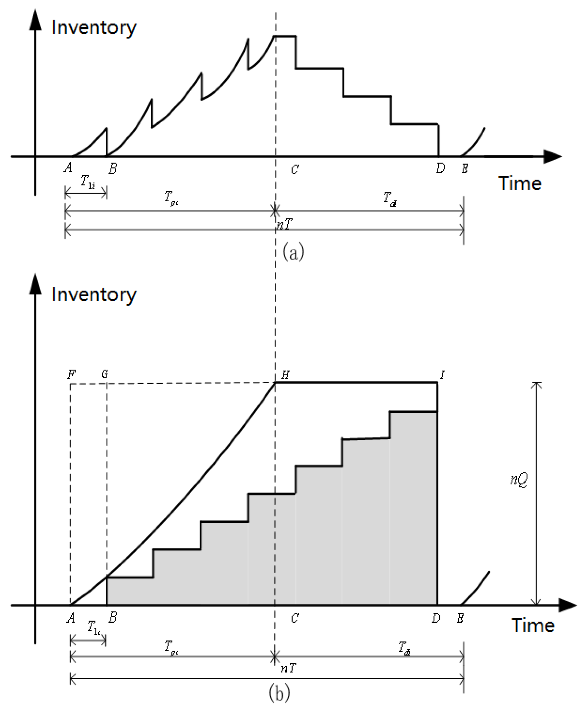
When the employees’ working behavior has Wright learning characteristics, the actual inventory level of the OEM supplier changes with time in a production cycle, as shown in Figure 2a. When the OEM supplier does not supply to the OEM brand enterprise, the time-varying cumulative inventory of the OEM supplier can be indicated by the solid line in Figure 2b. When the OEM supplier supplies to the OEM brand enterprise, the cumulative supply inventory of the OEM supplier can be indicated by the shaded part in Figure 2b.

According to the Wright learning curve theory, the production time of the xth product is $T_x=T_1{x}^{-b}$, in which $T_1$ is the time needed to complete the first product. The relationship between the learning coefficient $b$ and learning efficiency $\phi$ satisfied $b=-\log (\phi )/\log (2)$. The $\phi$ range is between 50% and 100% and the corresponding $b$ range is between 1 and 0.

Let the production time of the first product be $K$. Under the Wright learning theory, the total working hours of a batch of products are:

$$t(X)={\displaystyle {\int }_0^{X}K{x}^{-b}\mathrm{d}x}=\frac{K{x}^{1-b}}{1-b}.$$

(11)

According to Equation (11), in the ith cycle, the production time $T_{iQ}$ required for the first batch of quantity products is:

$$T_{iQ}={\displaystyle {\int }_{(i-1)nQ}^{Q+(i-1)nQ}{T}_1{m}^{-b}\mathrm{d}}m=\frac{T_1{Q}^{1-b}\left\{{[1+(i-1)n]}^{1-b}-{[(i-1)n]}^{1-b}\right\}}{1-b}.$$

(12)

In the ith cycle, the total production time $T_{pi}$ is:

$$T_{pi}={\displaystyle {\int }_{(i-1)nQ}^{inQ}{T}_1{m}^{-b}\mathrm{d}}m=\frac{T_1{(nQ)}^{1-b}[i^{1-b}-{(i-1)}^{1-b}]}{1-b}.$$

(13)

According to [13], when the OEM supplier does not supply to the OEM brand company, the variance of Equation (12) can be obtained. The cumulative inventory level of the OEM supplier is as follows:

$$I(t)={\left\{\frac{t(1-b)}{T_1[i^{1-b}-{(i-1)}^{1-b}]}\right\}}^{\frac{1}{1-b}}.$$

(14)

In Figure 2, the time length of CD is $nT-T_{pi}-(T-T_{iQ})$, the area of quadrilateral CDIH is $nQ\left[nT\right.-T_{pi}\left.-(T-T_{iQ})\right]$, the average inventory of the OEM supplier in non-production time is as follows:

$$nQ\left\{\frac{(n-1)(1-\gamma )Q}{\tilde{D}}\right.-\frac{T_1{(nQ)}^{1-b}[i^{1-b}-{(i-1)}^{1-b}]}{1-b}+\left.\frac{T_1{Q}^{1-b}\left\{{[1+(i-1)n]}^{1-b}-{[(i-1)n]}^{1-b}\right\}}{1-b}\right\}.$$

(15)

The area of the approximate triangle ACH is: ${\displaystyle {\int }_0^{T_{pi}}I(t)}\mathrm{d}t=\frac{T_1[i^{1-b}-{(i-1)}^{1-b}]{(nQ)}^{2-b}}{2-b}$.

In Figure 2b, the area of the non-shaded part is equal to the area of the approximate triangle ACH plus the area of the quadrilateral CDIH minus the area of the shaded part, thus the inventory cost of the OEM supplier in the ith cycle is as follows:

$$\begin{array}{l}I{C}_{vi}=h_v\frac{T_1[i^{1-b}-{(i-1)}^{1-b}]{(nQ)}^{2-b}}{2-b}+h_{v}nQ\frac{T_1{Q}^{1-b}\left\{{[1+(i-1)n]}^{1-b}-{[(i-1)n]}^{1-b}\right\}}{1-b}+\\ h_{v}nQ\left[\frac{(n-1)(1-\gamma )Q}{\tilde{D}}-\frac{T_1{(nQ)}^{1-b}[i^{1-b}-{(i-1)}^{1-b}]}{1-b}\right]-h_v\frac{n(n-1)(1-\gamma )Q^2}{2\tilde{D}}\end{array}.$$

(16)

Under immediate productivity, the total cost of the OEM supplier in the ith cycle is:

$$\begin{array}{l}T{C}_i^{\mathrm{IW}}(n,Q)\\ =S_v+vnQ\gamma +c\frac{T_1{(nQ)}^{1-b}[i^{1-b}-{(i-1)}^{1-b}]}{1-b}+h_{v}nQ\frac{T_1{Q}^{1-b}\left\{{[1+(i-1)n]}^{1-b}-{[(i-1)n]}^{1-b}\right\}}{1-b}\\ +h_v\frac{T_1[i^{1-b}-{(i-1)}^{1-b}]{(nQ)}^{2-b}}{2-b}+h_{v}nQ\left[\frac{(n-1)(1-\gamma )Q}{2\tilde{D}}-\frac{T_1{(nQ)}^{1-b}[i^{1-b}-{(i-1)}^{1-b}]}{1-b}\right]\end{array}.$$

(17)

The first item in Equation (17) is setup cost; the second item is defective quality assurance cost; the third item is production cost; and the fourth, fifth and sixth items are storage cost. Setup cost is the preparation and adjustment costs incurred in self-made production materials, it usually includes the costs of preparing work orders, arranging operations, preparing before production, and quality acceptance. Defective quality assurance cost are production losses caused by product quality defects. Production cost, also known as manufacturing cost, refers to the cost of production activities, that is, the cost incurred by an enterprise to produce products. Storage cost refers to all the costs incurred after materials are stored in the warehouse for a certain period of time, that is, the costs incurred to maintain inventory.

In Equation (17), the demand is fuzzy, so the cost of the whole production–inventory system is also fuzzy after considering the cost of the OEM brand enterprise. After calculating the average cost of the fuzzy system, the inverse fuzzification is needed. The average annual cost of the inverse fuzzification of the production–inventory system in the ith cycle is as follows:

$$\begin{array}{l}{U}_i^{\mathrm{IW}}(n,Q)=\frac{D+({\Delta }_2-{\Delta }_1)/4}{1-\gamma }\left\{\frac{S_v+S_B+nF}{nQ}+v\gamma +\vartheta +c\frac{T_1{(nQ)}^{-b}[i^{1-b}-{(i-1)}^{1-b}]}{1-b}\right.\\ -h_v\frac{T_1[i^{1-b}-{(i-1)}^{1-b}]{(nQ)}^{1-b}}{(2-b)(1-b)}\left.+h_v\frac{T_1{Q}^{1-b}\left\{{[1+(i-1)n]}^{1-b}-{[(i-1)n]}^{1-b}\right\}}{1-b}\right\}\\ +\frac{(n-1)h_{v}Q}{2}+\frac{h_B(1-\gamma )Q}{2}\end{array}.$$

(18)

Property 3.

For fixed $n$, when $i>1$, $n>1$, $U_i^{\mathrm{IW}}(n,Q)$ is convex in $Q$. There exists a unique $Q^{\ast }(n)$ making $U_i^{\mathrm{IW}}(n,Q)$ minimization.

Proof of Property 3.

Taking the first and second partial derivatives of $U_i^{\mathrm{IW}}(n,Q)$ with respect to $Q$, we have

$$\begin{array}{l}\frac{\partial U_i^{\mathrm{IW}}(n,Q)}{\partial Q}=\frac{D+({\Delta }_2-{\Delta }_1)/4}{1-\gamma }\left\{-\frac{S_v+S_B+nF}{n{Q}^2}\right.+c(-b)\frac{T_1{n}^{-b}{Q}^{-b-1}[i^{1-b}-{(i-1)}^{1-b}]}{1-b}\\ -h_v\frac{T_1[i^{1-b}-{(i-1)}^{1-b}]n^{1-b}{Q}^{-b}}{(2-b)}\left.+h_v{T}_1{Q}^{-b}\left\{{[1+(i-1)n]}^{1-b}-{[(i-1)n]}^{1-b}\right\}\right\}+\frac{(n-1)h_v}{2}+\frac{h_B(1-\gamma )}{2},\\ \frac{{\partial }^2{U}_i^{\mathrm{IW}}(n,Q)}{\partial Q^2}=\frac{D+({\Delta }_2-{\Delta }_1)/4}{1-\gamma }\left\{\frac{2(S_v+S_B+nF)}{n{Q}^3}\right.+cb(1+b)\frac{T_1{n}^{-b}{Q}^{-b-2}[i^{1-b}-{(i-1)}^{1-b}]}{1-b}\\ +\frac{h_{v}b{T}_1{Q}^{-b-1}[i^{1-b}{n}^{1-b}-{(i-1)}^{1-b}{n}^{1-b}]}{(2-b)}\left.-\frac{(2-b)b{h}_v{T}_1{Q}^{-b-1}\left\{{[1+(i-1)n]}^{1-b}-{[(i-1)n]}^{1-b}\right\}}{(2-b)}\right\}.\end{array}$$

When $i>1$, $n>1$, obviously $\frac{{\partial }^2{U}_i^{\mathrm{IW}}(n,Q)}{\partial Q^2}>0$. By letting $\frac{\partial U_i^{\mathrm{w}}(n,Q)}{\partial Q}=0$, using the one-dimensional search method, $Q^{\ast }(n)$ can be obtained.

When the workers’ work behavior has Wright learning characteristics, the number of the OEM supplier supplying to the OEM brand is an integer, and the optimal shipments should also satisfy Equations (9) and (10). □

5.2. Joint Optimization Model under Wright (AW) Average Productivity (Model 3)

Model 2 adopts the method of instant productivity in the process of modeling, and the productivity varies from moment to moment. In this section, the average productivity method is used. In any production cycle, the average productivity is used in the production cycle. According to Equation (13), the production time of the OEM supplier in the ith cycle is as follows:

$$T_{pi}^{\mathrm{AW}}={\displaystyle {\int }_{(i-1)nQ}^{inQ}{T}_1{m}^{-b}\mathrm{d}}m=\frac{T_1{(nQ)}^{1-b}\left[i^{1-b}-{(i-1)}^{1-b}\right]}{1-b},$$

(19)

According to the definition of average productivity, the average productivity of quantity $Q_p$ of products produced by the OEM supplier in the ith cycle is:

$$\overline{P^{\mathrm{AW}}}=\frac{Q_p}{T_{pi}^{\mathrm{AW}}}=\frac{{(nQ)}^b(1-b)}{T_1\left[i^{1-b}-{(i-1)}^{1-b}\right]},$$

(20)

By replacing $P$ within Equation (8), it can be concluded that the average annual cost of an integrated production–inventory system based on average productivity is as follows:

$$\begin{array}{l}{U}_i^{\mathrm{AW}}(n,Q)=[D+\frac{1}{4}({\Delta }_2-{\Delta }_1)]\left\{\frac{S_B+S_v+nF}{nQ(1-\gamma )}+\right.\frac{\vartheta +v\gamma }{1-\gamma }+\frac{c{T}_1{(nQ)}^{-b}\left[i^{1-b}-{(i-1)}^{1-b}\right]}{(1-b)(1-\gamma )}+\\ \left.\frac{h_v{n}^{-b}{Q}^{1-b}(2-n)T_1\left[i^{1-b}-{(i-1)}^{1-b}\right]}{2(1-b)(1-\gamma )}\right\}+\frac{h_{B}Q(1-\gamma )}{2}+h_{v}Q\frac{(n-1)}{2}\end{array},$$

(21)

The optimal shipments $n^{\ast }$ and lot size $Q^{\ast }$ can be obtained by solving the algorithm described in Section 5.

5.3. Joint Optimization Model under Cognitive Learning and Skill Learning (JGLCM) (Model 4)

Section 5.1 and Section 5.2 establish a cost model with the Wright learning characteristics of employees’ activity behavior. When considering the learning characteristics of an employee’s activity behavior, the cognitive learning process is neglected or the cognitive learning process is simply mixed with the skill learning process. This section divides the learning characteristics of employees’ work behavior into cognitive learning and skill learning.

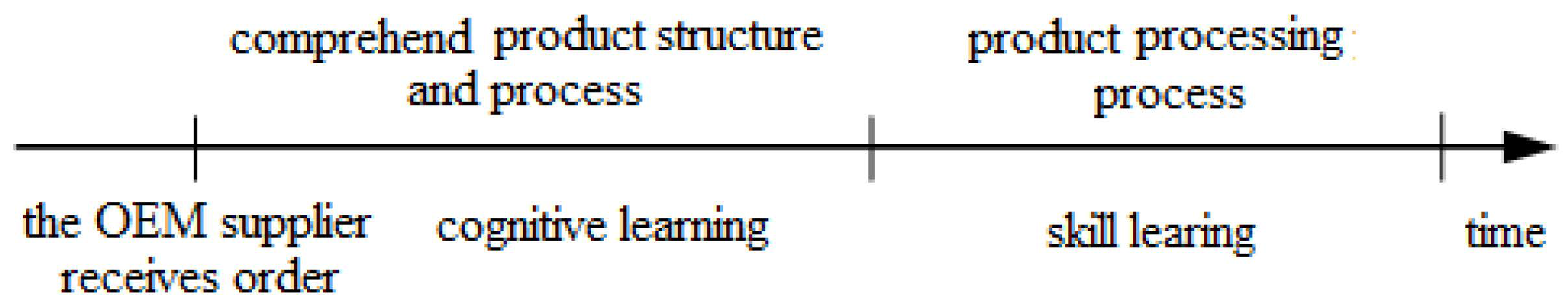
The cognitive learning characteristics of an employee’s work behavior refer to the learning process of explicit and tacit knowledge in the process of work. Cognitive learning is mainly a process of information exchange, in which information is acquired through perception, attention, memory, and understanding. Employees’ job-related behavior has the characteristics of skill learning, which means that the individual’s skill proficiency level grows higher and higher in the process of job-related activities. Figure 3 shows the cognitive learning and skill learning processes involved in employees’ job behavior.

Dar-el et al. [26] extended the Wright learning curve based on the cognitive learning and skill learning characteristics of employees’ work behavior and put forward a dual-phase learning curve model under cognitive learning and skill learning, which is abbreviated as DPLCM. When the learning characteristics of employees’ work behavior conform to the DPLCM model, the required work hours for completing the xth product are:

$$T_x=(T_1^c+T_1^m)x^{-b^{\ast }}=T_1^c{x}^{-b_c}+T_1^m{x}^{-b_m},$$

(22)

The production time $T_1^c$ required to complete the first product in Form 21 when there are only cognitive learning characteristics for employees’ work behavior. The production time $T_1^m$ required to complete the first product for employees with only skill learning characteristics. The relationship between compound learning coefficient $b^{\ast }$ and cognitive learning coefficient $b_c$ and skill learning coefficient $b_m$ is satisfied (23).

$$b^{\ast }=b_c-\frac{\log \left[(\hslash +n^{b_c-b_m})/(\hslash +1)\right]}{\log (n)},$$

(23)

In Equation (23), $\hslash =T_1^c/T_1^m$. Jaber and Glock [16] improved Dar-el’s model by dividing the initial production time and put forward the Jaber–Glock learning curve model, which is abbreviated as JGLCM. Through the simulation analysis of a large amount of data, it was found that the improved JGLCM is more suitable for the actual situation. When the learning characteristics of an employee’s work behavior conform to the JGLCM model, the time required to complete the xth product is:

$$T_x=\alpha T_1{x}^{-b_c}+(1-\alpha )T_1{x}^{-b_m},$$

(24)

In Equation (24), $\alpha$ indicates the proportion of time spent on cognitive learning, $1-\alpha$ indicates the proportion of time spent on skill learning. Let $ƛ=\alpha /(1-\alpha )$; in this paper $ƛ$ is called the initial cognitive skill coefficient, which is abbreviated as the cognitive skill coefficient.

When the learning characteristics of employees’ job behavior conform to the JGLCM model, the production time required to complete the number of products in the first cycle is as follows:

$$\begin{array}{l}{T}_{pi}^{\mathrm{JGCM}}={\displaystyle {\int }_{(i-1)Q_p}^{i{Q}_p}\left[\alpha T_1{x}^{-b_c}+(1-\alpha )T_1{x}^{-b_m}\right]\mathrm{d}}x\\ =\frac{\alpha T_1{Q}_p^{1-b_c}\left[i^{1-b_c}-{(i-1)}^{1-b_c}\right]}{1-b_c}+\frac{(1-\alpha )T_1{Q}_p^{1-b_m}\left[i^{1-b_m}-{(i-1)}^{1-b_m}\right]}{1-b_m}\end{array},$$

(25)

The average productivity of quantities $Q_p$ completed in the xth cycle:

$$\overline{P^{\mathrm{JGCM}}}=\frac{Q_p}{T_{pi}^{\mathrm{JGCM}}}=\frac{(1-b_m)(1-b_c)}{\alpha T_1(1-b_m)Q_p^{-b_c}\left[i^{1-b_c}-{(i-1)}^{1-b_c}\right]+(1-\alpha )T_1(1-b_c)Q_p^{-b_m}\left[i^{1-b_m}-{(i-1)}^{1-b_m}\right]}$$

(26)

When the learning characteristics of employees’ activity behavior conform to the JGLCM model, the average annual cost of the inverse fuzzification of an integrated production–inventory system can be obtained by replacing $P$ with $\overline{P^{\mathrm{JGCM}}}$ in Equation (8).

$$\begin{array}{l}{U}_i^{\mathrm{JGCM}}(n,Q)=[D+\frac{1}{4}({\Delta }_2-{\Delta }_1)]\left\{\frac{S_B+S_v+nF}{nQ(1-\gamma )}\right.+\frac{\vartheta +v\gamma }{1-\gamma }+\\ \frac{c}{\overline{P^{\mathrm{JGCM}}}(1-\gamma )}\left.+\frac{h_{v}Q(2-n)}{2\overline{P^{\mathrm{JGCM}}}(1-\gamma )}\right\}+\frac{h_{B}Q(1-\gamma )}{2}+h_{v}Q\frac{(n-1)}{2}\end{array},$$

(27)

The optimal shipments $n^{\ast }$ and lot size $Q^{\ast }$ can be obtained by solving the algorithm described in Section 5.

5.4. Joint Optimization Model under Improved Cognitive Learning and Skill Learning (FCLCM) (Model 5)

In the whole production process, there is a part of production time that is not affected by cognitive learning and skill learning. This part of production time is the shortest time to ensure the completion of product work. Based on this, this paper improves the JGLCM model and constructs the Fu–Chen learning curve model, which is briefly referred to as FCLCM. When the learning characteristics of employees’ work behavior conform to the FCLCM model, the time required to complete the xth product is:

$$T_x=\delta T_1+\beta T_1{x}^{-b_c}+(1-\beta -\delta )T_1{x}^{-b_m},$$

(28)

In Equation (28), $T_1$ represents the production time required to complete the first product when the employees’ work behavior does not have learning characteristics. $\delta$ represents the proportion of time spent completing a product in which there is neither cognitive learning nor skill learning. $\beta$ represents the proportion of time spent on cognitive learning and $1-\beta -\delta$ represents the proportion of time spent on skill learning. At the time $\delta =0$, the FCLCM model degenerated into the JGLCM model. It can be considered that the JGLCM model is a special case of the FCLCM model.

When the learning characteristics of employees’ job behavior conform to the FCLCM model, the production time required to complete the number of $Q_p$ products in the xth cycle is as follows:

$$\begin{array}{l}{T}_{pi}^{\mathrm{FCCM}}={\displaystyle {\int }_{(i-1)Q_p}^{i{Q}_p}\left[\delta T_1+\beta T_1{x}^{-b_c}+(1-\beta -\delta )T_1{x}^{-b_m}\right]\mathrm{d}}x\\ =\delta T_1{Q}_p+\frac{\beta T_1{Q}_p^{1-b_c}\left[i^{1-b_c}-{(i-1)}^{1-b_c}\right]}{1-b_c}+\frac{(1-\beta -\delta )T_1{Q}_p^{1-b_m}\left[i^{1-b_m}-{(i-1)}^{1-b_m}\right]}{1-b_m}\end{array},$$

(29)

Under the learning effect of FCLCM, the average productivity of $Q_p$ quantity of products completed in the xth cycle is:

$$\begin{array}{l}\overline{P^{\mathrm{FCCM}}}=\frac{Q_p}{T_{pi}^{\mathrm{FCCM}}}\\ =\frac{(1-b_m)(1-b_c)}{\delta T_1(1-b_m)(1-b_c)+\beta T_1{Q}_p^{-b_c}(1-b_m)\left[i^{1-b_c}-{(i-1)}^{1-b_c}\right]+(1-\beta -\delta )(1-b_c)T_1{Q}_p^{-b_m}\left[i^{1-b_m}-{(i-1)}^{1-b_m}\right]}\end{array},$$

(30)

The average annual cost of the inverse fuzzification of the integrated production–inventory system under the learning effect of FCLCM can be obtained by replacing $P$ with $\overline{P^{\mathrm{JGCM}}}$ in Equation (8).

$$\begin{array}{l}{U}_i^{\mathrm{FCCM}}(n,Q)=[D+\frac{1}{4}({\Delta }_2-{\Delta }_1)]\left\{\frac{S_B+S_v+nF}{nQ(1-\gamma )}\right.+\frac{\vartheta +v\gamma }{1-\gamma }+\frac{c}{\overline{P^{\mathrm{FCCM}}}(1-\gamma )}\\ \left.+\frac{h_{v}Q(2-n)}{2\overline{P^{\mathrm{FCCM}}}(1-\gamma )}\right\}+\frac{h_{B}Q(1-\gamma )}{2}+h_{v}Q\frac{(n-1)}{2}\end{array},$$

(31)

Property 4.

$\overline{P^{\mathrm{AW}}}>\overline{P^{\mathrm{JGCM}}}>\overline{P^{\mathrm{FCCM}}}$.

Proof of Property 4.

From the analysis of the following examples, it is clear that Property 1 is valid. □

6. Solution Algorithm of Production–Inventory Joint Optimization Model under FCLCM

Since $U_i^{\mathrm{IW}}(n,Q)$, $U_i^{\mathrm{AW}}(n,Q)$, $U_i^{\mathrm{JGCM}}(n,Q)$, and $U_i^{\mathrm{FCCM}}(n,Q)$ has high non-linearity, it is impossible to give the analytic solution of the optimal shipments $n^{\ast }$ and the lot size $Q^{\ast }$. The algorithm for solving $U_i^{\mathrm{IW}}(n,Q)$, $U_i^{\mathrm{AW}}(n,Q)$, $U_i^{\mathrm{JGCM}}(n,Q)$, and $U_i^{\mathrm{FCCM}}(n,Q)$ are the same, here we only give the solution algorithm to $U_i^{\mathrm{FCCM}}(n,Q)$.

Step 1: Set $i=1$;

Step 2: Set $Z_1(n,Q)=\frac{\partial U_i^{\mathrm{FCCM}}(n,Q)}{\partial n}$, $Z_2(n,Q)=\frac{\partial U_i^{\mathrm{FCCM}}(n,Q)}{\partial Q}$; the allowable error is $e$; and $(n(j),Q(j))$ represents the value of the jth iteration substitution $(n,Q)$;

Step 3: Given the initial value $(n(j),Q(j))$, from the beginning $j=1$;

Step 4: Calculate $Z_1(n(j),Q(j))$ and $Z_2(n(j),Q(j))$ separately;

Step 5: If $Z_1(n(j),Q(j))<e$, $Z_2(n(j),Q(j))<e$, go to Step 6, otherwise go to Step 7;

Step 6: The optimal shipments $n^{\ast }=n(j)$ and the lot size $Q^{\ast }=Q(j)$;

Step 7: Calculate $Z_1(n(j),Q(j))$, $Z_2(n(j),Q(j))$ and the partial derivative at $(n(j),Q(j))$, respectively,

$$I_j=\left(\begin{array}{l}{\left.\frac{\partial Z_1(n,Q)}{\partial n}\right|}_{(n,Q)=(n(j),Q(j))}{\left.\frac{\partial Z_1(n,Q)}{\partial n}\right|}_{(n,Q)=(n(j),Q(j))}\\ {\left.\frac{\partial Z_2(n,Q)}{\partial n}\right|}_{(n,Q)=(n(j),Q(j))}{\left.\frac{\partial Z_2(n,Q)}{\partial n}\right|}_{(n,Q)=(n(j),Q(j))}\end{array}\right);$$

Step 8: Calculate the tangents at the intersection points $(n(j),Q(j))$ of two surfaces, set $Z_1(n(j+1),Q(j+1))=0$ and $Z_2(n(j+1),Q(j+1))=0$, so that the next iteration point $(n(j+1),Q(j+1))$ can be obtained, and then return to Step 4, until the optimal solution $(n^{\ast },Q^{\ast })$ is obtained;

Step 9: Substitute $(n^{\ast },Q^{\ast })$ into $U_i^{\mathrm{FCCM}}(n,Q)$, so $U_i^{\ast \mathrm{FCCM}}(n^{\ast },Q^{\ast })$ is available;

Step 10: Set $i=i+1$;

Step 11: Repeat steps 2–9 until $i=N$ ($N$ is the number of production cycles after the learning curve is stable, which is the optimal production cycle, determined after testing);

Step 12: When the learning curve is stable, the $(n^{\ast },Q^{\ast })$ is available, and then the optimal annual average cost $U_i^{\ast \mathrm{FCCM}}(n^{\ast },Q^{\ast })$ can be obtained.

7. Parameter Setting and Comparative Analysis

7.1. Parameter Setting

Because of commercial confidentiality considerations, the data of case analysis are simulated data, rather than the real enterprise data. According to the documents [11,14], the following are set: productivity, $P=160,000$ (double/year); triangular fuzzy demand, $\tilde{D}=\left(46,000, 49,000, 56,000\right)$ (double/year), of which 49,000 (double/year) is the average demand, 46,000 (double/year) is the lower limit of demand, 56,000 (double/year) is the upper limit of demand; production preparation cost, $S_v=300$ (USD/year); ordering fee, $S_B=100$ (USD/year); fixed cost of each transportation, $F=25$ (USD/time); the OEM supplier unit storage cost, $h_v=2$ (USD/double/year); OEM brand merchant unit storage cost, $h_B=5$ (USD/double/year); brand enterprise unit quality inspection cost, $\vartheta =0.5$ (USD/double); the OEM supplier defect quality assurance cost, $v=30$ (USD/double); defect rate $\gamma =0.02$; annual production cost, $c=300,000$.

For the learning coefficient, the cognitive learning rate is ${\varphi }_c=70\%$ and the skill learning rate is ${\varphi }_m=90\%$, that is, the learning coefficients $b_c=0.514$ and $b_m=0.152$. To facilitate the comparison between Model 3 and Model 4, set $\hslash =ƛ$, the learning coefficient in Model 3 is calculated by Equation (22). In this paper, we take $\alpha =0.68$, $ƛ$ = 2.125, and obtain the learning coefficient under WLC as $b=0.295$. In Model 5, $\delta =0.01$ and $\beta =0.65$.

7.2. Comparative Analysis

When an employee’s activity behavior does not have learning characteristics, according to the proof process of Property 1 and the applicable conditions of the optimal number of deliveries are the optimal number of deliveries $n^{\ast }=7$ (times) and the optimal single quantity of deliveries are $Q^{\ast }=782$ (double), the optimal average annual cost is USD 162,506.09.

When the employee’s job behavior has learning characteristics, the optimal number of times of supply, the optimal single quantity of supply, and the average annual cost of the first 30 production cycle Models 2, 3, 4, and 5 can be obtained by solving the $U^{\mathrm{FCCM}}(n,Q)$ algorithm (

Table 2. Optimal solutions of Models 2, 3, 4, and 5.

	Model 2 (IW)			Model 3 (AW)			Model 4 (JGLCM)			Model 5 (FCLCM)
$\mathit{i}$	${\mathit{n}}^{\ast }$	${\mathit{Q}}^{\ast }$	${\mathit{U}}^{\mathbf{IW}}(\mathit{n},\mathit{Q})$	${\mathit{n}}^{\ast }$	${\mathit{Q}}^{\ast }$	${\mathit{U}}^{\mathbf{AW}}(\mathit{n},\mathit{Q})$	${\mathit{n}}^{\ast }$	${\mathit{Q}}^{\ast }$	${\mathit{U}}^{\mathbf{JGCM}}(\mathit{n},\mathit{Q})$	${\mathit{n}}^{\ast }$	${\mathit{Q}}^{\ast }$	${\mathit{U}}^{\mathbf{FCCM}}(\mathit{n},\mathit{Q})$
1	7	911	78,498.61	7	917	78,488.01	6	915	79,265.39	7	912	80,709.86
2	6	923	74,675.71	6	924	74,693.69	6	920	76,389.6	6	917	77,788.99
3	6	925	73,724.33	6	926	73,740.74	6	922	75,643.15	6	919	77,013.83
4	6	927	73,179.66	6	927	73,194.8	6	923	75,202.86	6	920	76,555.40
5	6	927	72,807.54	6	928	72,821.71	6	923	74,895.34	6	920	76,234.68
6	6	928	72,529.54	6	928	72,542.95	6	924	74,661.44	6	921	75,990.45
7	6	928	72,310.15	6	929	72,322.94	6	924	74,474.02	6	921	75,794.58
8	6	929	72,130.43	6	929	72,142.71	6	924	74,318.46	6	922	75,631.88
9	6	929	71,979.19	6	929	71,991.02	6	925	74,186.00	6	922	75,493.26
10	6	929	71,849.26	6	930	71,860.72	6	925	74,070.99	6	922	75,372.85
11	6	930	71,735.83	6	930	71,746.95	6	925	73,969.63	6	922	75,266.67
12	6	930	71,635.51	6	930	71,646.33	6	925	73,879.17	6	923	75,171.88
13	6	930	71,545.82	6	930	71,556.38	5	925	73,797.64	6	923	75,086.42
14	5	930	71,464.92	5	930	71,475.23	5	926	73,723.53	6	923	75,008.71
15	5	930	71,391.37	5	930	71,401.46	5	926	73,655.68	6	923	74,937.54
16	5	931	71,324.07	5	931	71,333.97	5	926	73,593.18	6	923	74,871.96
17	5	931	71,262.14	5	931	71,271.85	5	926	73,535.29	6	923	74,811.21
18	5	931	71,204.85	5	931	71,214.39	5	926	73,481.42	6	923	74,754.67
19	5	931	71,151.63	5	931	71,161.00	5	926	73,431.09	6	924	74,701.83
20	5	931	71,101.98	5	931	71,111.21	5	926	73,383.89	5	924	74,652.26
21	5	931	71,055.50	5	931	71,064.59	5	926	73,339.46	5	924	74,605.60
22	5	931	71,011.85	5	931	71,020.81	5	926	73,297.54	5	924	74,561.56
23	5	931	70,970.74	5	931	70,979.58	5	927	73,257.86	5	924	74,519.88
24	5	931	70,931.92	5	931	70,940.63	5	927	73,220.22	5	924	74,480.32
25	5	931	70,895.16	5	931	70,903.77	5	927	73,184.42	5	924	74,442.70
26	5	932	70,860.28	5	932	70,868.78	5	927	73,150.31	5	924	74,406.85
27	5	932	70,827.12	5	932	70,835.53	5	927	73,117.75	5	924	74,372.62
28	5	932	70,795.53	5	932	70,803.84	5	927	73,086.61	5	924	74,339.88
29	5	932	70,765.39	5	932	70,773.61	5	927	73,056.77	5	924	74,308.52
30	5	932	70,736.58	5	932	70,744.71	5	927	73,028.15	5	924	74,278.42

). By comparing the data of the first production cycle of Models 2, 3, 4, and 5 with Model 1, it was found that the average cost of the system is much less than that of the case without learning characteristics and the optimal quantities of single supply are greater than those of the case without learning characteristics. This is due to the higher than average productivity of employees with learning characteristics. The OEM supplier is encouraged to produce more products because of their learning characteristics.

By comparing Model 2 (IW) and Model 3 (AW) in Table 2, it can be seen that in the first production cycle, the average annual cost of the system obtained by the average productivity method is slightly lower than the average annual cost of the system obtained by the instant productivity method, but in other production cycles, the average annual cost obtained by the average productivity method is slightly higher than that obtained by the instant productivity method. The results of calculating the optimal annual average cost of the production–inventory system by using the average productivity method or the instant productivity method are almost the same. This also shows that it is reasonable to use the average productivity method to calculate the annual average cost of the production–inventory system when the employees’ activities have cognitive learning characteristics and skills learning characteristics.

When the production tends to be stable, the optimal number of deliveries and the single quantity of deliveries in Model 2 and Model 3 are the same. When the production tends to be stable, no matter what the situation is, the optimal number of supply times is the same. In the AW case, the single quantity of supply is the largest, and in the FCLCM case, the single quantity of supply is the smallest. This is due to the maximum amount of production in Wright learning situations. As shown in Table 1, the annual average cost of Model 3 in the 30th production cycle is USD 7743.30 lower than that in the 1st production cycle. The average annual cost of Model 4 in the 30th production cycle is USD 6237.24 lower than that in the 1st production cycle. With the continuation of production, the average cost of the system becomes smaller and smaller, the optimal single supply volume becomes larger and larger, and the optimal number of times of supply becomes smaller and smaller. When production tends to be stable, the 30 production cycles are selected to explore the effects of cognitive learning coefficient, skill learning coefficient, and $\lambda$ change on Models 2, 3, 4, and 5.

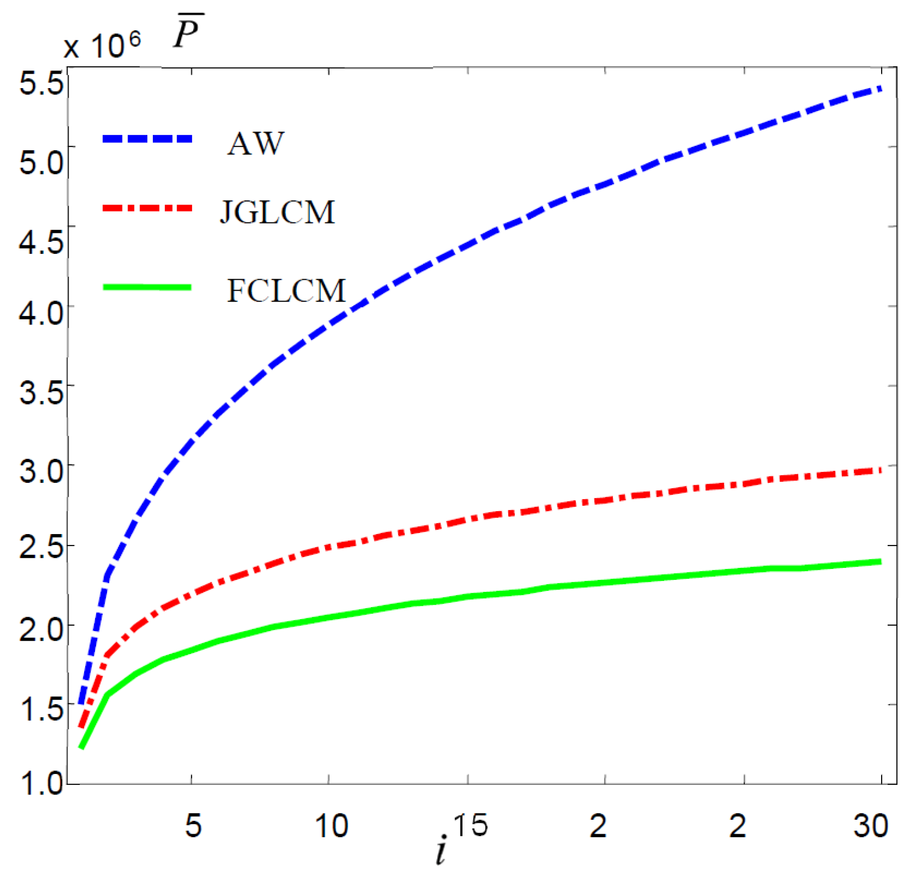
The OEM supplier’s productivity varies with the existence of learning characteristics of an employee’s job behavior. According to Figure 4, Figure 6 and Figure 8, Wright learning has the highest average productivity, followed by JGLCM and FCLCM. Compared with JGLCM, AW has learning integration, while JGLCM has learning disassembly. JGLCM further subdivides learning and weakens part of the learning effect, so the average productivity is smaller. Compared with JGLCM, FCLCM contains a part of production time that does not have a learning effect. It further dismantles learning and further weakens the learning effect of some assignments, thus the average productivity of FCLCM is the lowest. In theory, according to the Wright learning curve theory, the production time of the xth product is $T_x=T_1{x}^{-b}$, no matter in AW or JGLCM, only the production goes on, the production time of the product is close to zero, but in actual production, there is a minimum production time to complete a product. This part of production time has no learning effect, so the FCLCM in Model 5 is closer to the real-life complexity.

(1)

Impact of production cycle changes

Figure 4 shows the change in average productivity in different production cycles with different learning characteristics. In the early stage of operation, the learning effect of employees’ operation behavior makes productivity increase greatly. In the later stage of operation, the productivity increases slowly in JGLCM and FCLCM situations and the productivity difference tends to be stable. Overall, the average productivity growth rate becomes smaller and smaller, and the growth rate in the AW case is greater than that in the JGLCM case and FCLCM case.

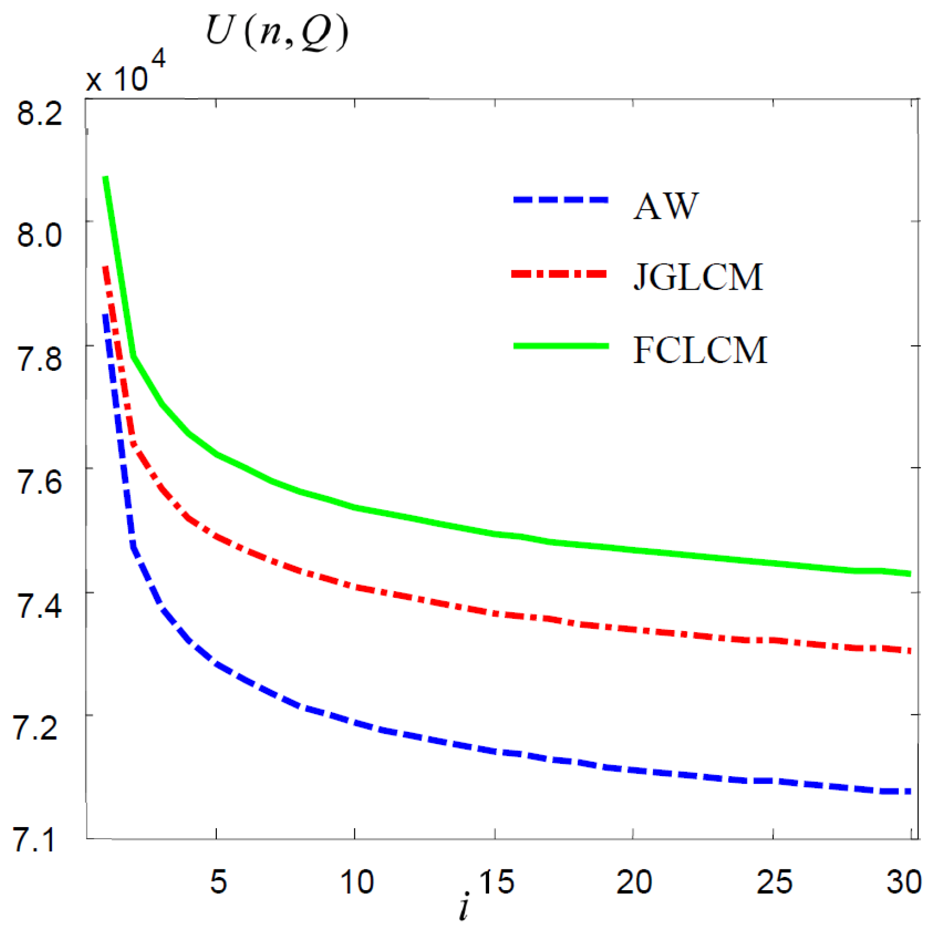
Figure 5 shows the impact of different production cycles on the optimal annual average cost of the production–inventory system. In the early stage of operation, the annual average cost of the system decreases significantly due to the significant increase in productivity. The learning effect in employees’ activity behavior plays a significant role in reducing costs. In the latter stage, because the operation tends to be stable, the increase in productivity is not obvious, resulting in a decrease in the annual average cost of the system is not obvious. Compared with the AW case, the JGLCM case and the FCLCM case tend to be stable ahead of time. The difference between the average annual cost of FCLCM and JGLCM in the latter stage of the operation is stability, which is caused by the production time in which there is no learning effect.

(2)

The influence of the change in cognitive learning coefficient

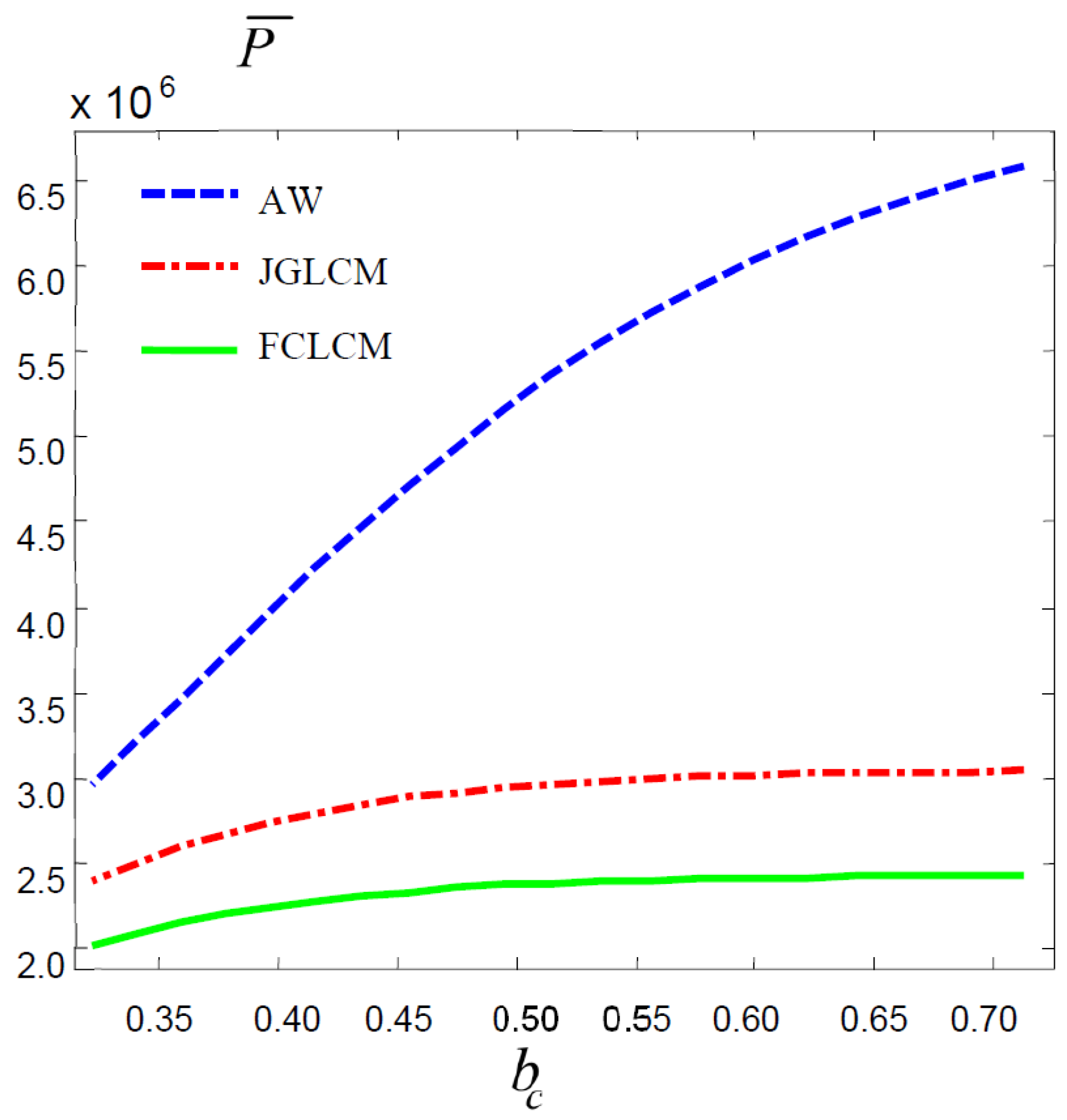
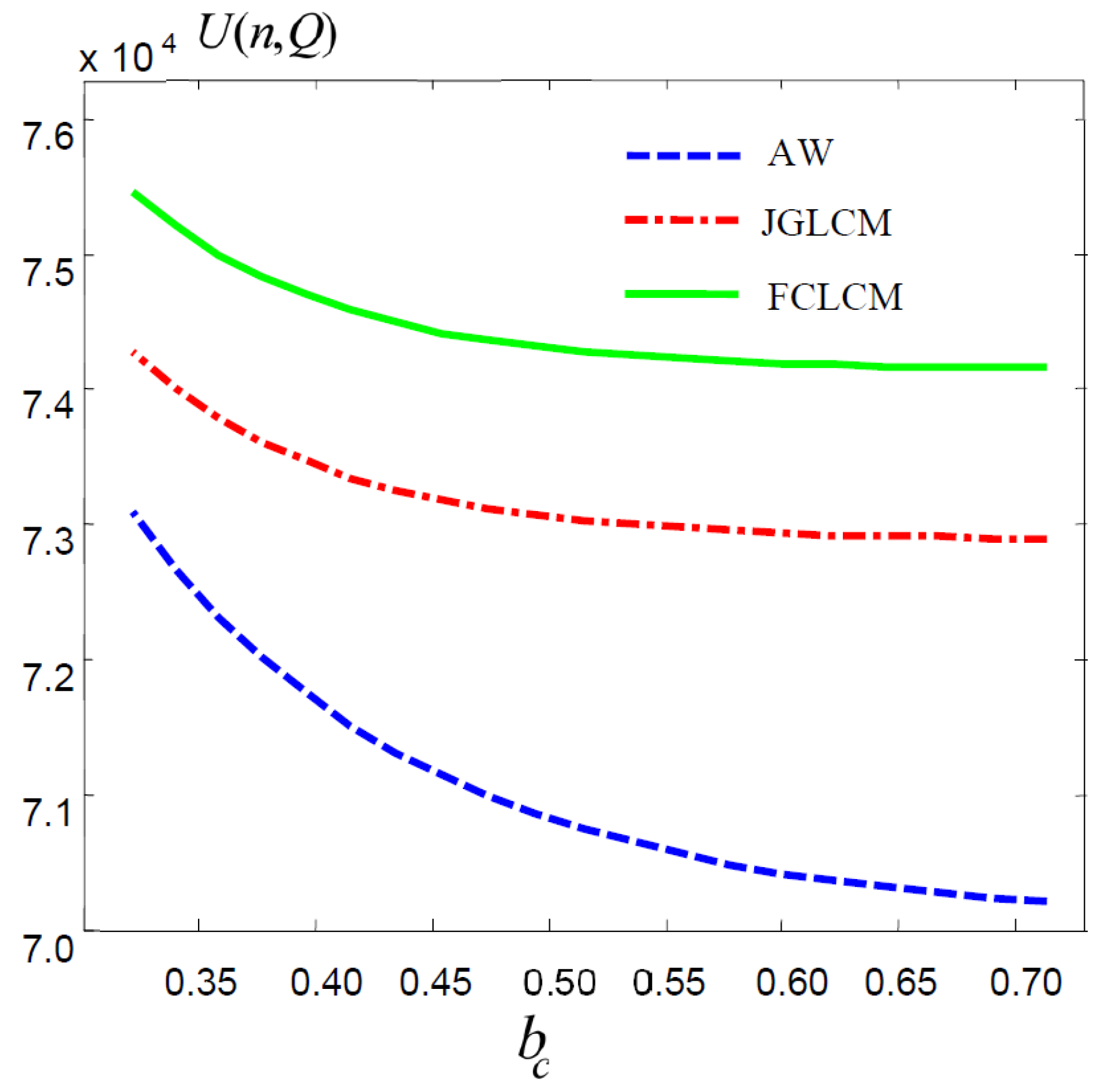
The change of cognitive learning coefficient $b_c$ can be transformed into the change of overall learning coefficient by Equation (22). Figure 6 shows that with the increase of cognitive learning coefficient $b_c$ in employees’ work behavior, cognitive learning efficiency becomes smaller and smaller, and productivity increases in AW, JGLCM, and FCLCM, but the productivity increases in AW are larger than that in JGLCM and FCLCM, and the differences between AW and JGLCM and FCLCM become larger and larger. In the three cases, the increase in productivity becomes smaller and smaller. When cognitive learning coefficient is $b_c>0.5$, the productivity of JGLCM and FCLCM remains stable, while that of AW continues to increase. The productivity in the JGLCM case is higher than that in the FCLCM case because there is no learning effect in part of the production time in the FCLCM case. The change in cognitive learning coefficient leads to the change in productivity and further affects the change in annual average cost. With the increase in cognitive learning coefficient, $b_c$, the annual average cost of all three kinds of cases decreases and the rate of decline becomes smaller and smaller (Figure 7). JGLCM and FCLCM tend to be stable before AW. The cost difference between the JGLCM case and AW case becomes bigger and bigger.

(3)

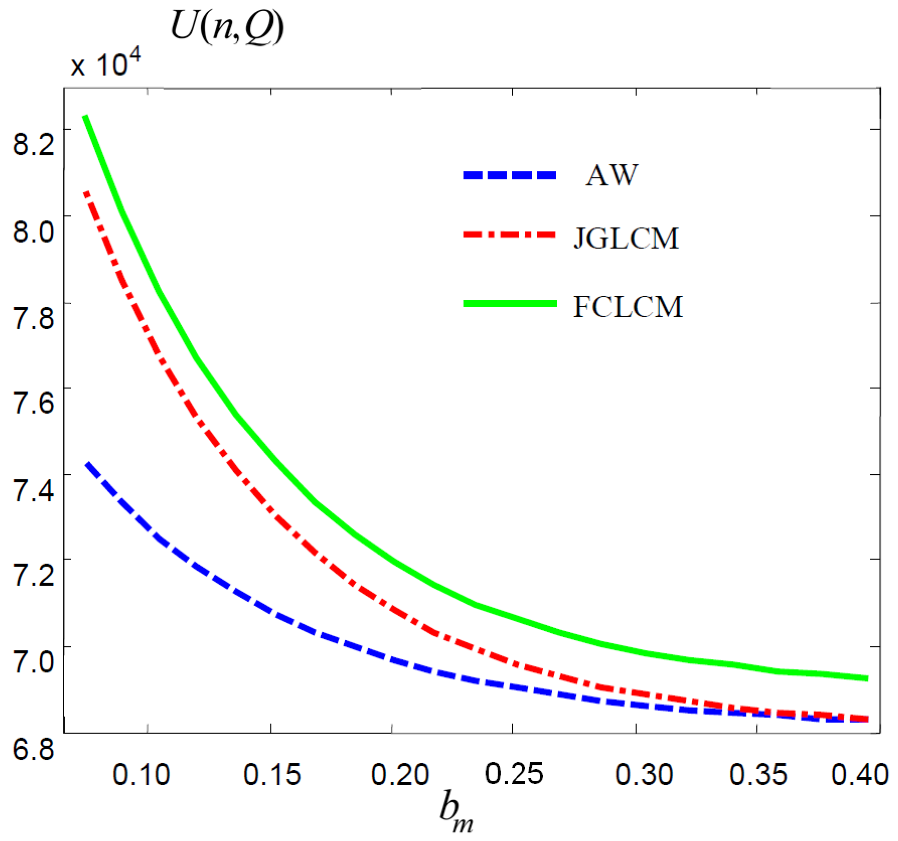
Impact of changes in skill learning coefficient

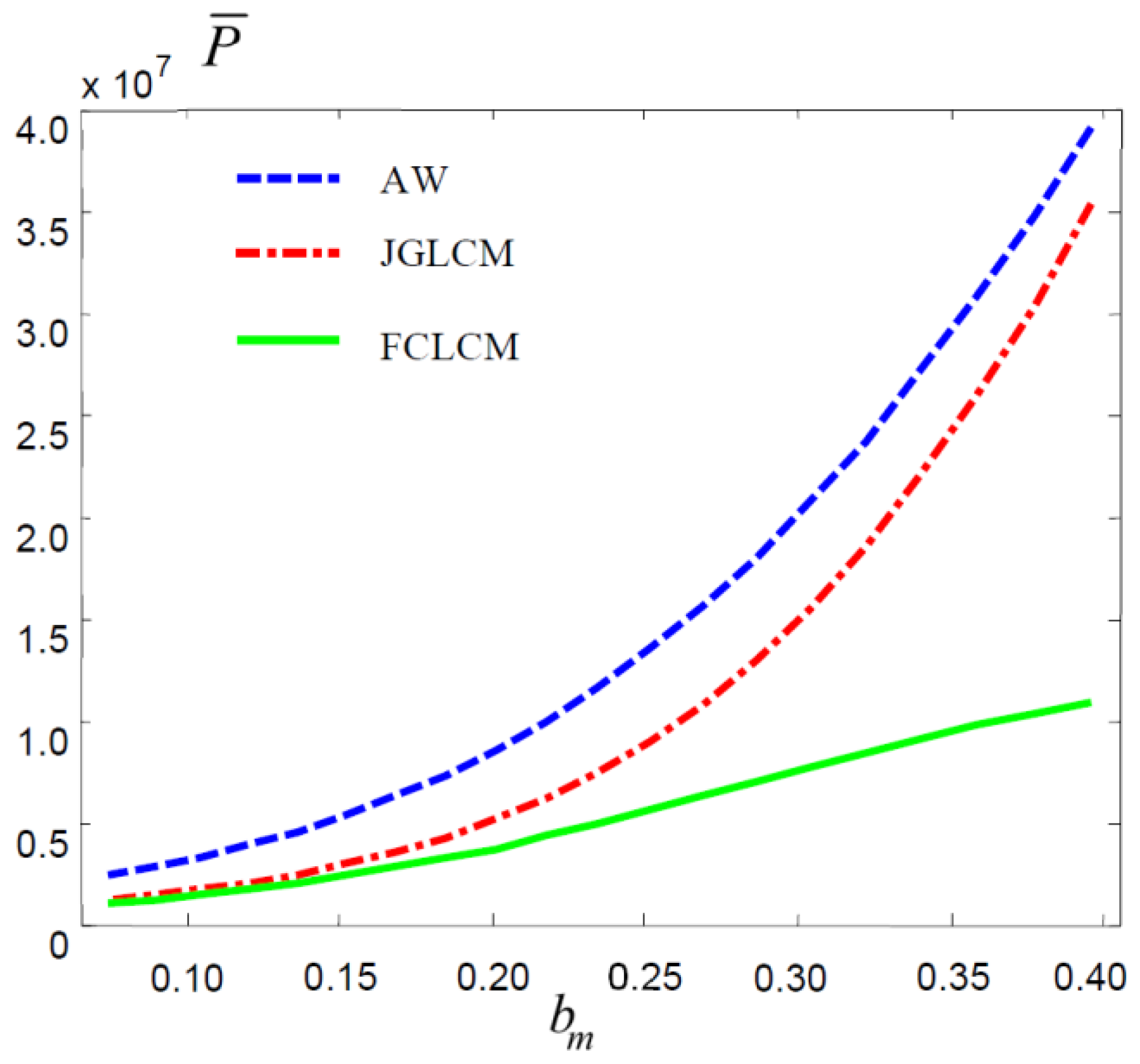
Figure 8 shows that with the increase in the skill learning coefficient, the average productivity increases in all three situations. At that time, the average productivity in AW and JGLCM cases has significantly increased process. In the AW case and JGLCM case, the average rate increases more and more, while in the FCLCM case, the average rate increases almost linearly. Figure 9 shows that with the increase of skill learning coefficients, the annual average cost of the three types of situations becomes smaller and smaller. The average annual cost in the AW case and JGLCM case converged and the average annual cost in the FCLCM case and JGLCM case maintained a stable difference, which was caused by the absence of learning effect in some activities. The annual average cost of the production–inventory system in the FCLCM case does not converge with that in the AW case and JGLCM case.

Observing the curve of Figure 7 and Figure 9 when the cost tends to be stable, the cognitive learning coefficient is less than the skill learning coefficient (0.4 < 0.6), that is, the cognitive learning rate is greater than the skill learning rate. The management implication is that when cognitive learning tends to stabilize, the cost reduction of improving skill learning is limited. Managers need to strengthen cognitive learning training for grass-root workers.

(4)

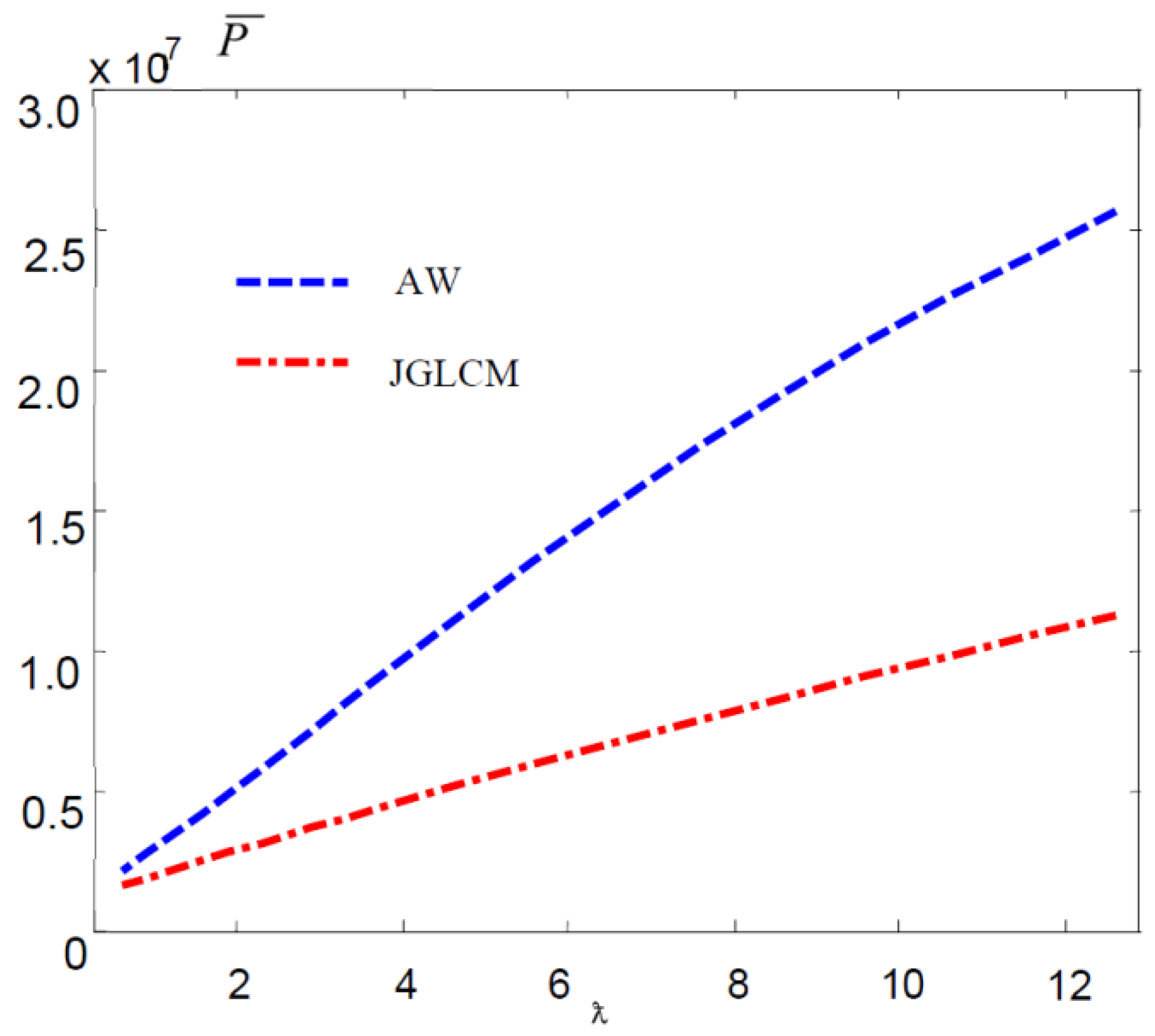
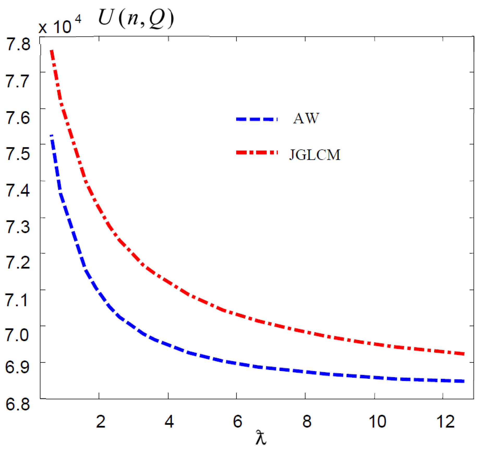
The influence of the change of recognition coefficient

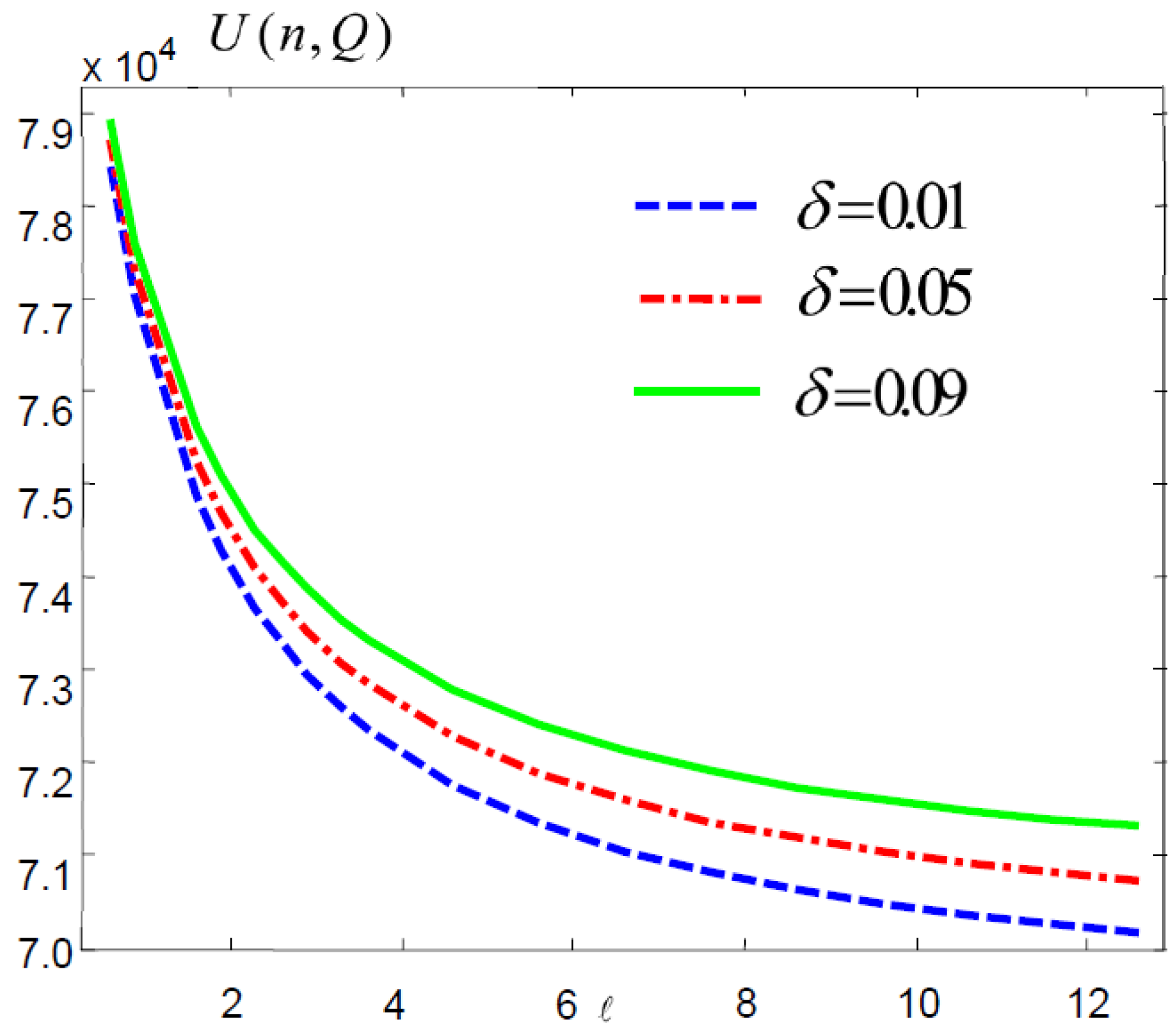
Figure 10 shows that the average productivity increases with the increase of $\lambda$ in the AW and JGLCM cases, and the difference between them also increases. As shown in Figure 11, the change of $\lambda$ in optimal cost in AW and JGLCM shows hyperbolic characteristics. The increase of $\lambda$ means that cognitive learning plays an increasingly important role in learning. When $b_c$ and $b_m$ stay unchanged, $\lambda$ increasing means an increase in $\alpha$. The decreasing trend of the optimal annual average cost caused by the increase of $\alpha$ is similar to that caused by the increase of $b_m$ on the optimal annual average cost.

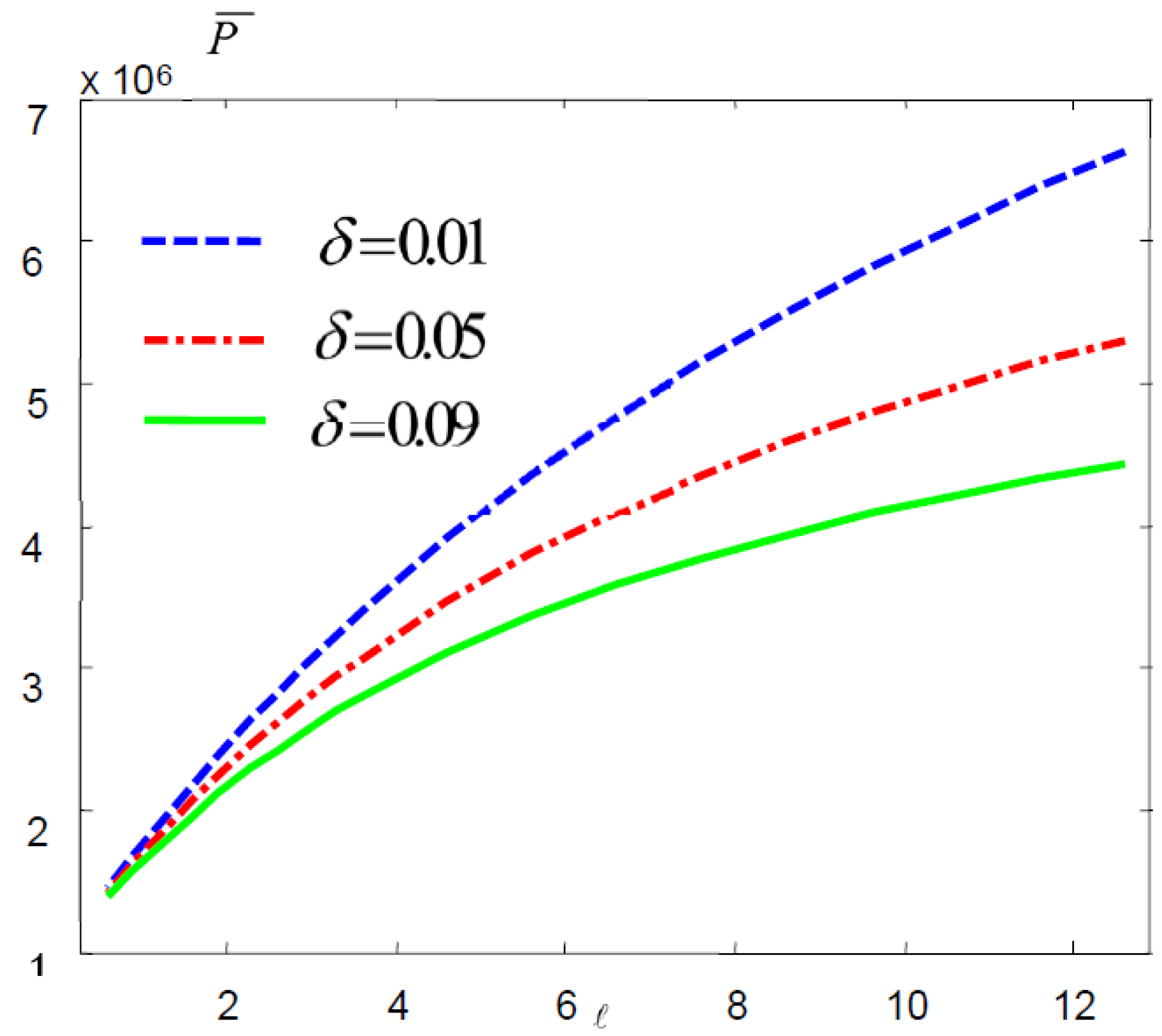
Given $\delta$, set $\ell =\beta /(1-\delta -\beta )$, to examine the impact of $\ell$ changes on average productivity and annual average cost in the case of FCLCM. Combining Figure 12 with Figure 13 $\delta$ means the smaller the production time without the learning effect, the larger the average productivity and the smaller the average annual cost. With $\ell$ increasing, the average productivity increases, the average annual cost decreases, and the incremental range of the average productivity decreases, which leads to the decrease in the average annual cost.

8. Managerial Insights

The learning characteristics of employees’ work behavior exist generally and objectively in production practice. The learning effect has an obvious influence on completion time and production cost. Therefore, enterprises need to consider the learning effect in the process of employees’ work when formulating a business strategy, a production plan, and salary design. This will ensure that the production plan formulated by enterprises is more in line with the current situation.

The insights of this paper for managers reveal that targeted induction training can help employees acquire the necessary skills needed for production as soon as possible and promote employees to integrate into the enterprise faster. The knowledge that employees gain causes the learning effect to play a key role in reducing costs in the early stage of production. Employee turnover is not conducive to the steady exertion of the learning effect on the improvement of productivity and the reduction of costs, so humanistic management measures should be taken to reduce employee turnover.

In the later stage of production, it is more and more difficult to improve production efficiency and reduce costs. It is not realistic to reduce production costs by learning effect. OEM suppliers need to invest more research and development (R&D) resources to produce new products to form a new learning effect. When enterprises renew their products, new learning effects emerge, which requires the retraining of old employees.

Compared with the skill learning training for production technicians, it is necessary to pay more attention to the training of cognitive learning. OEM suppliers need to strengthen the training of cognitive learning for production technicians. When cognitive learning tends to be stable, the cost reduction of improving skill learning is limited. Currently, it is not wise to invest in skill improvement.

9. Conclusions

Based on the dynamic change of productivity caused by the learning effect, this paper establishes five kinds of production–inventory joint optimization models, which are, in turn, non-learning effects, instant productivity under Wright learning, average productivity under Wright learning, cognitive learning, and skill learning. The cognitive learning (JGLCM) and skill learning (FCLCM) situations were improved. The production–inventory system consists of a brand enterprise and an OEM supplier. The main conclusions obtained by theoretical and numerical analysis include:

(1)

Based on cognitive learning and skill learning, FCLCM is constructed. By using FCLCM, the problem that the production time cannot be zero after production is stable is solved.

(2)

Compared with the JGLCM case, the AW case involves learning integration, while the JGLCM case involves learning disassembly. JGLCM further subdivides learning and weakens part of the learning effect, so the average productivity is smaller. Increasing productivity does not necessarily reduce the average cost of the system. When demand is stable, excessive productivity leads to the overstocking of inventory and increases the inventory holding cost.

(3)

The total cost under the learning effect is lower than that without the learning effect. The total cost under cognitive learning and skill learning is higher than that under Wright learning, but the optimal lot size under cognitive learning and skill learning is smaller than that under Wright learning. A learning effect plays an important role of increasing productivity and decreasing costs in the early stage, whereas after production tends to be stable, the role of a learning effect is very limited.

(4)

The increase in the cognitive learning coefficient and skill learning coefficient reduces the total cost of the production–inventory system. With the increase in cognitive learning coefficient, the gap between the total cost of cognitive learning and skill learning and that of Wright learning becomes smaller and smaller, and with the increase of the skill learning coefficient, the gap between the total cost of cognitive learning and skill learning and that of Wright learning becomes wider and wider. With the increase of the cognitive coefficient, the total cost of cognitive learning and skill learning and the total cost of Wright learning show hyperbolic characteristics. When cognitive learning tends to be stable, the cost reduction brought about by improving skill learning is limited.

The paper does not consider the impact of forgetfulness on employees’ work behavior. Forgetting occurs after production is interrupted. Forgetting causes the accumulated knowledge and skills in the production process to be lost. When production starts again, it cannot maintain the high-level operational advantage as at the end of the previous production. The impact of forgetting cannot be ignored. In the future, we will consider the impact of the forgetting characteristics of employees’ work behavior.

References

- Dmua, B.; Is, C.; Yh, D.; Wapd, C. Integrated procurement-production inventory model in supply chain: A systematic review. Oper. Res. Perspect. 2022, 9, 100221. [Google Scholar]
- Rahman, M.S.; Das, S.; Manna, A.K.; Shaikh, A.A.; Bhunia, A.K.; Cárdenas-Barrón, L.E.; Treviño-Garza, G.; Céspedes-Mota, A. A mathematical model of the production inventory problem for mixing liquid considering preservation Facility. Mathematics 2021, 9, 3166. [Google Scholar] [CrossRef]
- Sadeghi, H.; Golpra, H.; Khan, S. Optimal integrated production-inventory system considering shortages and discrete delivery orders. Comput. Ind. Eng. 2021, 156, 107233. [Google Scholar] [CrossRef]
- Elhafsi, M.; Fang, J.; Hamouda, E. Optimal production and inventory control of multi-class mixed backorder and lost sales demand class models. Eur. J. Oper. Res. 2021, 291, 147–161. [Google Scholar] [CrossRef]
- Chen, Z.; Bidanda, B. Sustainable manufacturing production-inventory decision of multiple factories with jit logistics, component recovery and emission control. Transp. Res. Part E Logist. Transp. Rev. 2019, 128, 356–383. [Google Scholar] [CrossRef]
- De, A.G.; Tijms, H.C.; Van, F.A. Approximations for the single-product production-inventory problem with compound Poisson demand and service-level constraints. Adv. Appl. Probab. 1984, 16, 378–401. [Google Scholar]
- Nambiar, M.; Wang, H.; Singhal, K. Dynamic inventory allocation with demand learning for seasonal goods. Prod. Oper. Manag. 2021, 30, 750–765. [Google Scholar] [CrossRef]
- Sepehri, A.; Mishra, U.; Sarkar, B. A sustainable production-inventory model with imperfect quality under preservation technology and quality improvement investment. J. Clean. Prod. 2021, 310, 127332. [Google Scholar] [CrossRef]
- Jaber, M.Y.; Guiffrida, A.L. Learning curves for processes generating defects requiring reworks. Eur. J. Oper. Res. 2005, 159, 663–672. [Google Scholar] [CrossRef]
- Jaber, M.Y.; Goyal, S.K.; Imran, M. Economic production quantity model for items with imperfect quality subject to learning effects. Int. J. Prod. Econ. 2008, 115, 143–150. [Google Scholar] [CrossRef]
- Salameh, M.K.; Jaber, M.Y. Economic production quantity model for items with imperfect quality. Int. J. Prod. Econ. 2000, 64, 59–64. [Google Scholar] [CrossRef]
- Khan, M.; Jaber, M.Y.; Guiffrida, A.L. The effect of human factors on the performance of a two level supply chain. Int. J. Prod. Res. 2012, 50, 517–533. [Google Scholar] [CrossRef]
- Khan, M.; Jaber, M.Y.; Ahmad, A.R. An integrated supply chain model with errors in quality inspection and learning in production. Omega 2014, 42, 16–24. [Google Scholar] [CrossRef]
- Huang, C.K. An optimal policy for a single-vendor single-buyer integrated production–inventory problem with process unreliability consideration. Int. J. Prod. Econ. 2004, 91, 91–98. [Google Scholar] [CrossRef]
- Mahata, G.C. A production-inventory model with imperfect production process and partial backlogging under learning considerations in fuzzy random environments. J. Intell. Manuf. 2017, 28, 883–897. [Google Scholar] [CrossRef]
- Jaber, M.Y.; Glock, C.H. A learning curve for tasks with cognitive and motor elements. Comput. Ind. Eng. 2013, 64, 866–871. [Google Scholar] [CrossRef]
- Atabaki, M.H.; Pasandideh, S.; Mohammadi, M. A hybrid invasive weed optimization for an imperfect, two-warehouse, lot-sizing problem. J. Model. Manag. 2020, 15, 1363–1387. [Google Scholar] [CrossRef]
- He, Q.; Li, S.; Xu, F.; Qiu, W. Deep-Processing Service and Pricing Decisions for Fresh Products with the Rate of Deterioration. Mathematics 2022, 10, 745. [Google Scholar] [CrossRef]
- De, S.K.; Bhattacharya, K. A pollution sensitive marxian production inventory model with deterioration under fuzzy system. J. Optim. Theory Appl. 2022, 192, 598–627. [Google Scholar] [CrossRef]
- Khanna, A.; Gautam, P.; Jaggi, C.K. Inventory Modeling for Deteriorating Imperfect Quality Items with Selling Price Dependent Demand and Shortage Backordering under Credit Financing. Int. J. Math. Eng. Manag. Sci. 2017, 2, 110–124. [Google Scholar] [CrossRef]
- Salas-Navarro, K.; Acevedo-Chedid, J.; Rquez, G.M.; Florez, W.F.; Ospina-Mateus, H.; Sana, S.S.; Cárdenas-Barrón, L.E. An EPQ inventory model considering an imperfect production system with probabilistic demand and collaborative approach. J. Adv. Manag. Res. 2019, 17, 282–304. [Google Scholar] [CrossRef]
- Kurdhi, N.A.; Nurhayati, R.A.; Wiyono, S.B.; Handajani, S.; Martini, T. A collaborative vendor-buyer production-inventory systems with imperfect quality items, inspection errors, and stochastic demand under budget capacity constraint: A Karush-Kuhn-Tucker conditions approach. IOP Conf. Ser. Mater. Sci. Eng. 2017, 166, 12013. [Google Scholar] [CrossRef] [Green Version]
- Hsu, J.T.; Hsu, L.F. An integrated single-vendor single-buyer production-inventory model for items with imperfect quality and inspection errors. Int. J. Ind. Eng. Comput. 2012, 3, 703–720. [Google Scholar] [CrossRef]
- Hsu, J.T.; Hsu, L.F. An integrated vendor-buyer inventory model with imperfect items and planned back ordering. Int. J. Adv. Manuf. Technol. 2013, 68, 2121–2132. [Google Scholar] [CrossRef]
- Pan, J.C.H.; Yang, M.F. Integrated inventory models with fuzzy annual demand and fuzzy production rate in a supply chain. Int. J. Prod. Res. 2008, 46, 753–770. [Google Scholar] [CrossRef]
- Darel, E.M.; Ayas, K.; Gilad, I. A dual-phase model for the individual learning process in industrial tasks. IIE Trans. 1995, 27, 265–271. [Google Scholar] [CrossRef]
- Goyal, S.K.; Huang, C.K.; Chen, K.C. A simple integrated production policy of an imperfect item for vendor and buyer. Prod. Plan. Control 2003, 14, 596–602. [Google Scholar] [CrossRef]
Figure 1.
Inventory level change and cumulative supply of OEM suppliers.
Figure 2.
Inventory level change and cumulative supply of the OEM supplier under WLC.
Figure 3.
Cognitive learning and skill learning process of employees’ homework behaviors.
Figure 4.
Impact of i on average productivity.
Figure 5.
Effect of i on optimal cost.
Figure 6.
Effect of bc change on average productivity.
Figure 7.
Effect of bc change on optimal cost.
Figure 8.
Effect of bm changes on average productivity.
Figure 9.
Effect of bm changes on optimal cost.
Figure 10.
Effect of changes on average productivity.
Figure 11.
Effect of changes on optimal cost.
Figure 12.
Figure 13.