
Artificial Bee Colony Algorithm with Nelder–Mead Method to Solve Nurse Scheduling Problem

 , , , and
Abstract
:1. Introduction
- A hybrid meta-heuristic algorithm, namely artificial bee colony optimization with Nelder–Mead Method, is proposed.
- The search capability of ABC is enriched with the aid of the Nelder–Mead method, which consists of search strategies such as midpoint, reflection, expansion, contraction, and shrinkage processes. These search strategies enhance the balance between exploration and exploitation.
- NM-ABC is implemented and tested on the nurse scheduling problem (NSPLib).
- The performance of NM-ABC is compared with that of some classical optimization algorithms.
2. Nurse Scheduling Problem
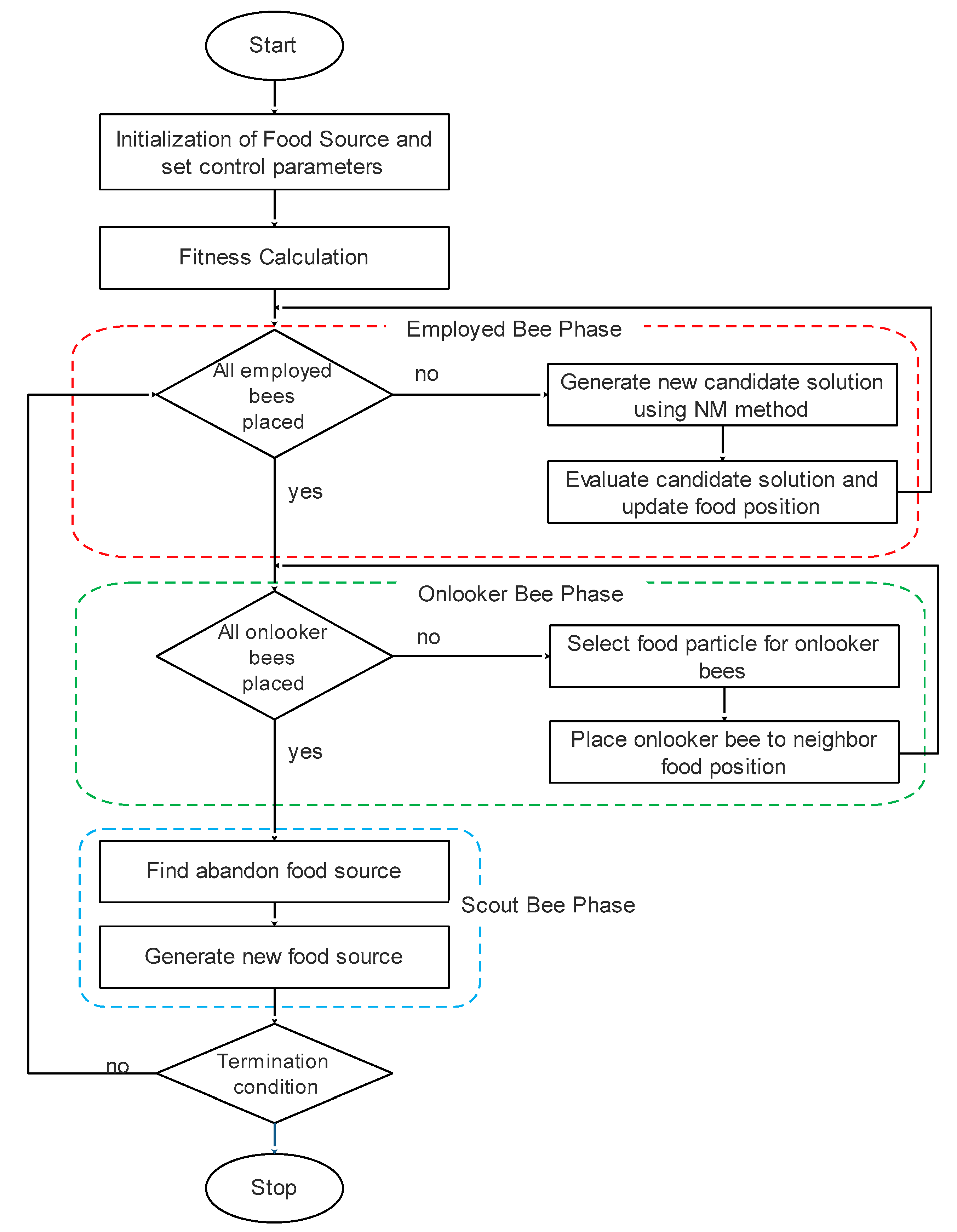
3. Proposed Algorithm
3.1. Artificial Bee Colony Algorithm
3.1.1. Initialization
3.1.2. Employed Bee Phase
3.1.3. Probability Calculation
| Algorithm 1: Probability calculation | |
| 1: | Fori = 1, 2, …, FS, do |
| 2: | Calculate probability values for the solution |
| 3: | |
| 4: | |
| 5: | End For |
3.1.4. Onlooker Bee Phase
3.1.5. Scout Bee Phase
3.2. Nelder–Mead Method
3.2.1. Midpoint (M)
3.2.2. Reflection (R)
3.2.3. Expansion (E)
3.2.4. Contraction (C)
3.2.5. Shrinkage (S)
| Algorithm 2: Nelder–Mead Method | |
| 1: | Produce new food source using modified Nelder–Mead Method |
| 2: | Let denote list of vertices |
| 3: | , μ, λ, and ζ are the constants of likeness, extension, shrinkage, and contraction |
| 4: | f is the fitness method to be reduced |
| 5: | For i = 1, 2, …, n + 1 vertices, do |
| 6: | Order the vertices from deepest fitness function f(v_1) to maximum fitness function f(〖v〗_(n + 1)) |
| 7: | |
| 8: | Calculate midpoint for best two vertices |
| 9: | , where i = 1, 2, …, n |
| 10: | Calculate reflection point v_r |
| 11: | |
| 12: | if then |
| 13: | and go to stopping criteria |
| 14: | End if |
| 15: | Calculate expansion point |
| 16: | if then |
| 17: | and go to stopping criteria |
| 18: | End if |
| 19: | if then |
| 20: | and go to stopping criteria |
| 21: | else |
| 22: | and go to stopping criteria |
| 23: | End if |
| 24: | Calculate contraction point |
| 25: | if then |
| 26: | Compute outside contraction |
| 27: | . |
| 28: | End if |
| 29: | if then |
| 30: | Compute inside contraction |
| 31: | . |
| 32: | End if |
| 33: | if then |
| 34: | Shrinkage is done between and the best vertex among and . |
| 35: | End if |
| 36: | if then |
| 37: | and go to Stopping criteria |
| 38: | else go to Shrinkage phase |
| 39: | End if |
| 40: | if then |
| 41: | and go to Stopping criteria |
| 42: | else go to the Shrinkage phase |
| 43: | End if |
| 44: | Calculate Shrinkage |
| 45: | Shrink close the best individual with new apices |
| 46: | , where i = 2, …, n + 1 |
| 47: | End for |
| 48: | Determine the new vertices of the simplex thus formed based on their fitness and continue with the process of the reflection phase |
3.3. Nelder–Mead Method-Based ABC (NM-ABC)
| Algorithm 3: NM-ABC | |
| 1: | Initialize the population |
| 2: | For i = 1, 2, …, FS, do |
| 3: | For j = 1, 2, …, S, do |
| 4: | Generate solution |
| 5: | |
| 6: | Where and are the min and max limit of the dimension |
| 7: | End for |
| 8: | Compute the objective of the population |
| 9: | |
| 10: | Repeat |
| 11: | { |
| 12: | Employed Bee Phase |
| 13: | For each food source do |
| 14: | Generate candidate solution using Equation (14) |
| 15: | Select between and |
| 16: | End For |
| 17: | Onlooker Bee Phase |
| 18: | Set r = 0 |
| 19: | While (r <= FS) |
| 20: | If rand(0,1) < using Algorithm 3 |
| 21: | Generate candidate solution by Algorithm 2 |
| 22: | Select between and |
| 23: | r = r + 1 |
| 24: | End if |
| 25: | End while |
| 26: | Scout Bee Phase |
| 27: | Abandon the food source , which cannot improve further using Equation (13) |
| 28: | Remember the best individual obtained so far |
| 29: | iter = iter + 1 |
| 30: | } |
| 31: | End for |
| 32: | Until iter = max FEs |
4. Experimental Results
4.1. Experimental Setup
4.2. Performance Metrics
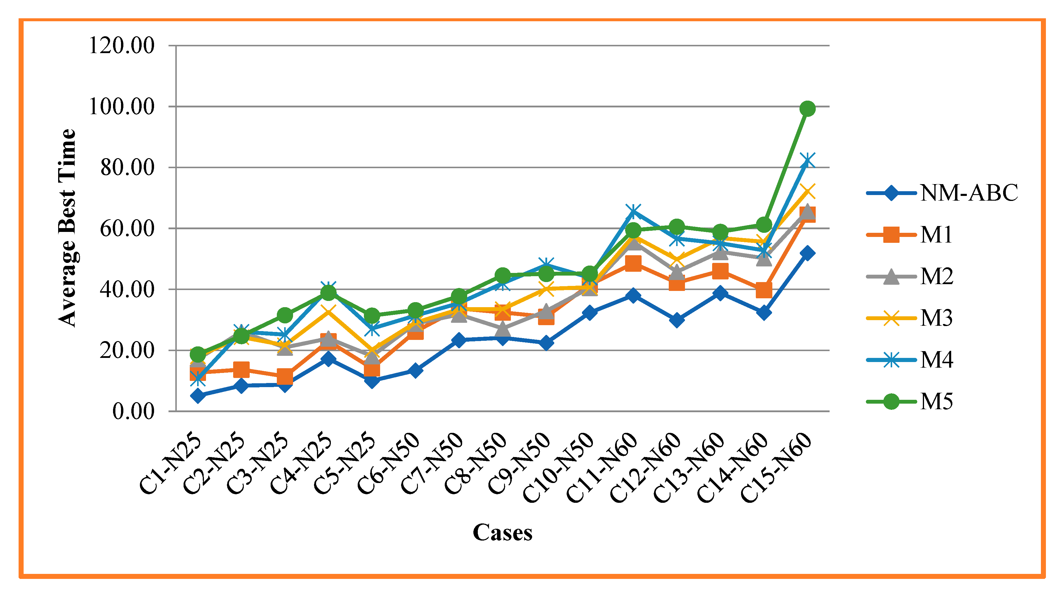
4.2.1. Average Best Time (ABT)
4.2.2. Standard Deviation
4.2.3. Least Error Rate
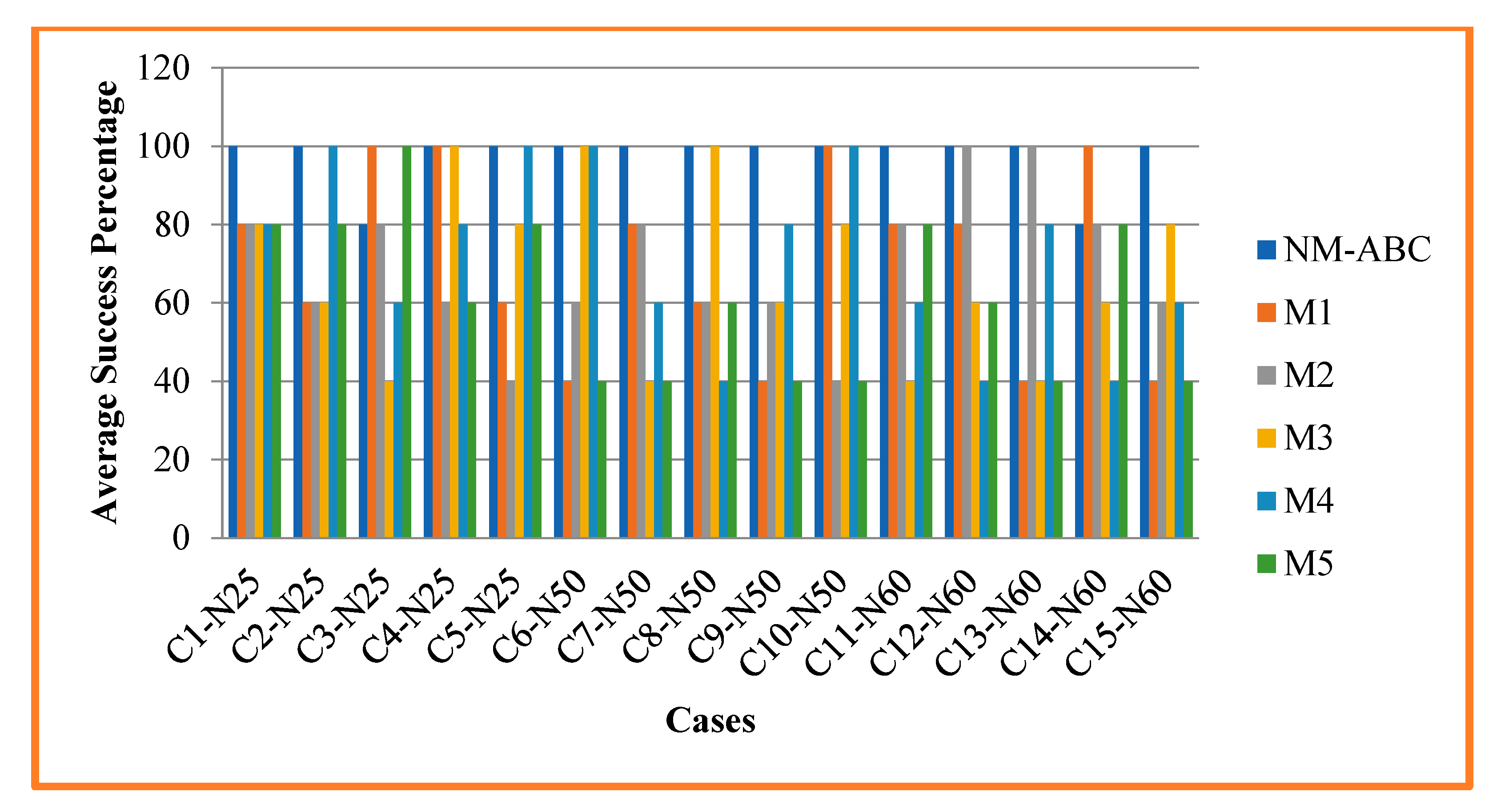
4.2.4. Success Percentage
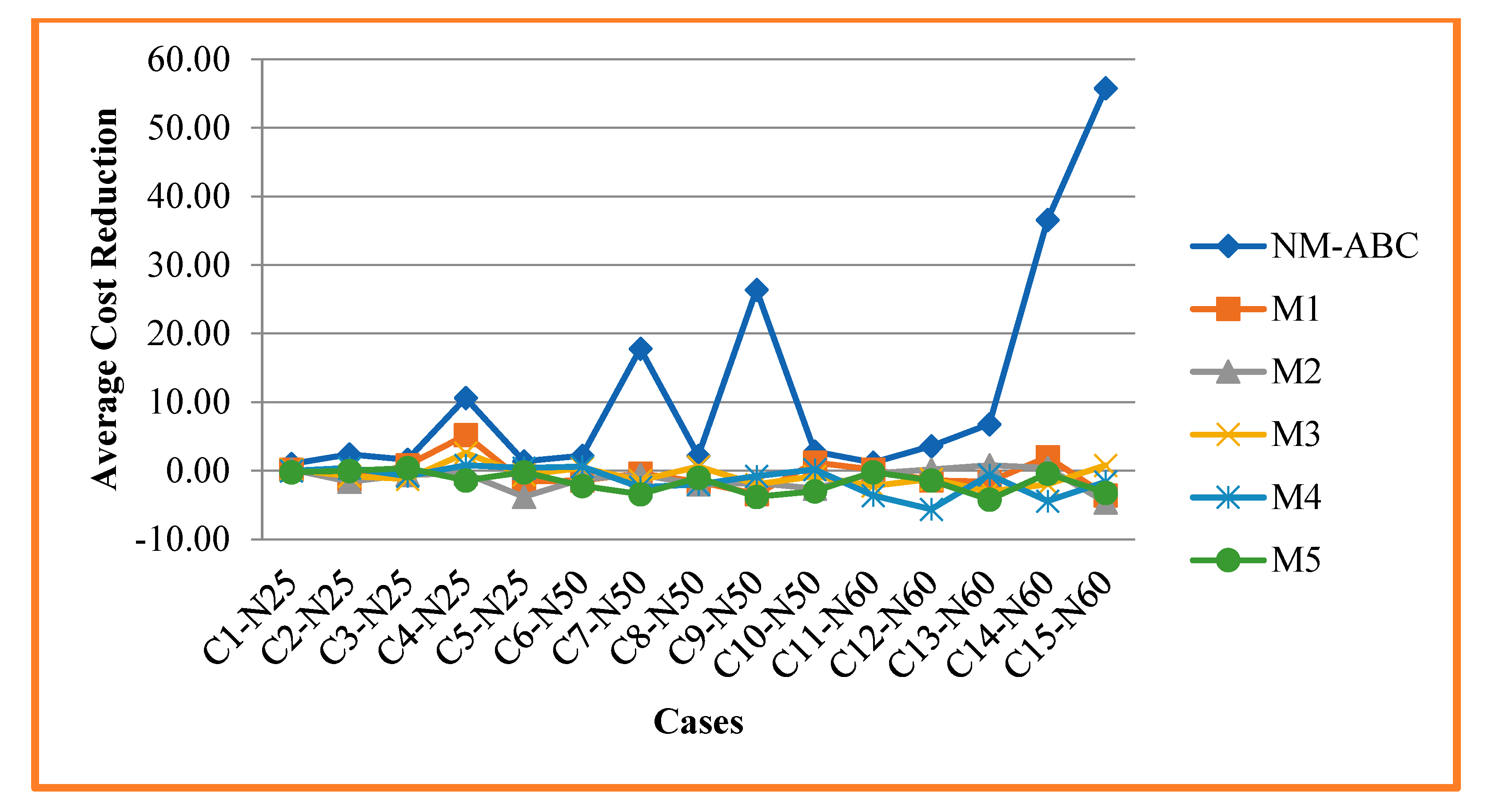
4.2.5. Cost Reduction
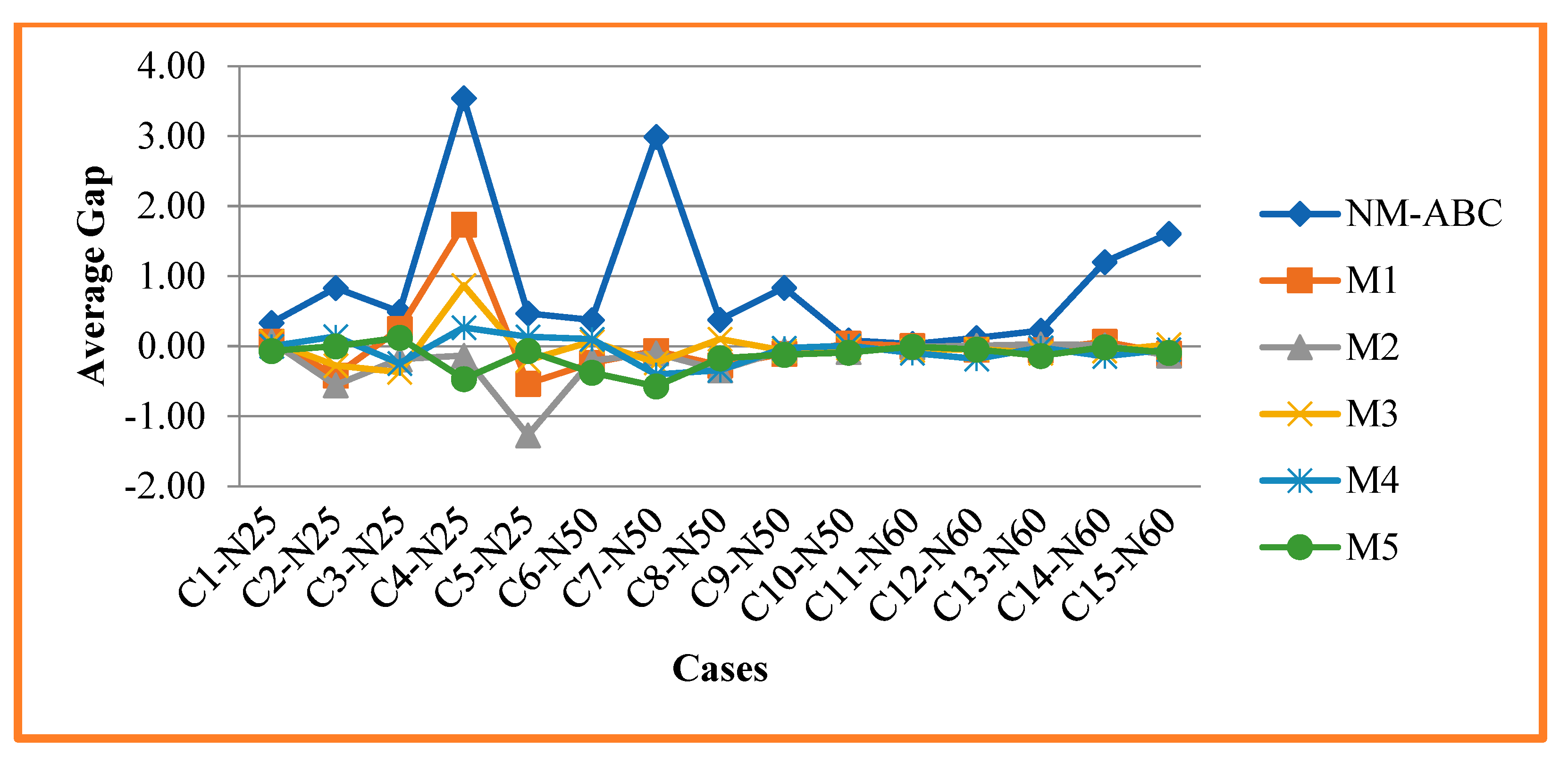
4.2.6. Gap
4.2.7. #Both Feasible Solution
4.2.8. #Feasible Solution
4.3. Experimental Result Analysis
5. Discussions
6. Conclusions
Author Contributions
Funding
Institutional Review Board Statement
Informed Consent Statement
Data Availability Statement
Conflicts of Interest
References
- Anwar, K.; Awadallah, M.A.; Khader, A.T.; Al-Betar, M.A. Hyper-heuristic approach for solving nurse rostering problem. In Proceedings of the 2014 IEEE Symposium on Computational Intelligence in Ensemble Learning (CIEL), Orlando, FL, USA, 9–12 December 2014. [Google Scholar]
- Awadallah, M.A.; Bolaji, A.L.; Al-Betar, M.A. A hybrid artificial bee colony for a nurse rostering problem. Appl. Soft Comput. 2015, 35, 726–739. [Google Scholar] [CrossRef]
- Constantino, A.A.; Landa-Silva, D.; de Melo, E.L.; de Mendonça, C.F.X.; Rizzato, D.B.; Romão, W. A heuristic algorithm based on multi-assignment procedures for nurse scheduling. Ann. Oper. Res. 2014, 218, 165–183. [Google Scholar] [CrossRef] [Green Version]
- Garey, M.R.; Johnson, D.S. Computers and Intractability: A Guide to the Theory of NP-Completeness; W.H. Freeman: San Francisco, CA, USA, 1979. [Google Scholar]
- Megeath, J.D. Successful hospital personnel scheduling. Interfaces 1978, 8, 55–60. [Google Scholar] [CrossRef]
- Musliu, N.; Gärtner, J.; Slany, W. Efficient generation of rotating workforce schedules. Discret. Appl. Math. 2002, 118, 85–98. [Google Scholar] [CrossRef] [Green Version]
- Millar, H.H.; Kiragu, M. Cyclic and non-cyclic scheduling of 12 h shift nurses by network programming. Eur. J. Oper. Res. 1998, 104, 582–592. [Google Scholar] [CrossRef]
- Burke, E.; de Causmaecker, P.; Berghe, G.V. A hybrid tabu search algorithm for the nurse rostering problem. In Simulated Evolution and Learning. SEAL 1998; Springer: Berlin/Heidelberg, Germany, 1998; pp. 187–194. [Google Scholar] [CrossRef]
- Legrain, A.; Omer, J.; Rosat, S. An online stochastic algorithm for a dynamic nurse scheduling problem. Eur. J. Oper. Res. 2020, 285, 196–210. [Google Scholar] [CrossRef] [Green Version]
- Özcan, E.; Bilgin, B.; Korkmaz, E.E. Hill climbers and mutational heuristics in hyperheuristics. In Parallel Problem Solving from Nature-PPSN IX; Springer: Berlin/Heidelberg, Germany, 2006; pp. 202–211. [Google Scholar]
- Cheang, B.; Li, H.; Lim, A.; Rodrigues, B. Nurse rostering problems—A bibliographic survey. Eur. J. Oper. Res. 2003, 151, 447–460. [Google Scholar] [CrossRef]
- Jaradat, G.M.; Al-Badareen, A.; Ayob, M.; Al-Smadi, M.; Al-Marashdeh, I.; Ash-Shuqran, M.; Al-Odat, E. Hybrid elitist-ant system for nurse-rostering problem. J. King Saud Univ. Comput. Inf. Sci. 2019, 31, 378–384. [Google Scholar] [CrossRef]
- Van den Bergh, J.; Beliën, J.; De Bruecker, P.; Demeulemeester, E.; De Boeck, L. Personnel scheduling: A literature review. Eur. J. Oper. Res. 2013, 226, 367–385. [Google Scholar] [CrossRef]
- Burke, E.K.; De Causmaecker, P.; Berghe, G.V.; Van Landeghem, H. The state of the art of nurse rostering. J. Sched. 2004, 7, 441–499. [Google Scholar] [CrossRef]
- Aickelin, U.; Dowsland, K.A. Exploiting problem structure in a genetic algorithm approach to a nurse rostering problem. J. Sched. 2000, 3, 139–153. [Google Scholar] [CrossRef] [Green Version]
- Burke, E.K.; Li, J.; Qu, R. Pareto-Based Optimization for Multi-objective Nurse Scheduling. Computer Science Technical Report No. NOTTCS-TR-2007-5. 2007. Available online: https://www.researchgate.net/publication/277291801_Pareto-Based_Optimization_for_Multi-objective_Nurse_Scheduling_Corresponding_author (accessed on 1 October 2021).
- Weil, G.; Heus, K.; Francois, P.; Poujade, M. Constraint programming for nurse scheduling. IEEE Eng. Med. Biol. Mag. 1995, 14, 417–422. [Google Scholar] [CrossRef]
- Brusco, M.J.; Jacobs, L.W. Cost analysis of alternative formulations for personnel scheduling in continuously operating organizations. Eur. J. Oper. Res. 1995, 86, 249–261. [Google Scholar] [CrossRef]
- Lourenço, H.R.; Martin, O.C.; Stützle, T. Iterated local search. In Handbook of Metaheuristics; Springer: New York, NY, USA, 2003; pp. 320–353. [Google Scholar]
- Warner, D.M.; Prawda, J. A mathematical programming model for scheduling nursing personnel in a hospital. Manag. Sci. 1972, 19 Pt 1, 411–422. [Google Scholar] [CrossRef]
- Kawanaka, H.; Yamamoto, K.; Yoshikawa, T.; Shinogi, T.; Tsuruoka, S. Genetic algorithm with the constraints for nurse scheduling problem. In Proceedings of the 2001 Congress on Evolutionary Computation (IEEE Cat. No.01TH8546), Seoul, Korea, 27–30 May 2001; Volume 2, pp. 1123–1130. [Google Scholar]
- Burke, E.K.; Li, J.; Qu, R. A hybrid model of integer programming and variable neighborhood search for highly-constrained nurse rostering problems. Eur. J. Oper. Res. 2010, 203, 484–493. [Google Scholar] [CrossRef]
- Kennedy, J. Particle swarm optimization. In Encyclopedia of Machine Learning; Springer: New York, NY, USA, 2011; pp. 760–766. [Google Scholar]
- Gutjahr, W.J.; Rauner, M.S. An ACO algorithm for a dynamic regional nurse-scheduling problem in Austria. Comput. Oper. Res. 2007, 34, 642–666. [Google Scholar] [CrossRef] [Green Version]
- Berrada, I.; Ferland, J.A.; Michelon, P. A multi-objective approach to nurse scheduling with both hard and soft constraints. Socio-Econ. Plan. Sci. 1996, 30, 183–193. [Google Scholar] [CrossRef]
- Burke, E.K.; Curtois, T.; Qu, R.; Berghe, G.V. A scatter search methodology for the nurse rostering problem. J. Oper. Res. Soc. 2010, 61, 1667–1679. [Google Scholar] [CrossRef] [Green Version]
- Todorovic, N.; Petrovic, S. Bee colony optimization algorithm for nurse rostering. IEEE Trans. Syst. Man Cybern. Syst. 2013, 43, 467–473. [Google Scholar] [CrossRef]
- Xu, Y.; Wang, X. An artificial bee colony algorithm for scheduling call centres with weekend-off fairness. Appl. Soft Comput. 2021, 109, 107542. [Google Scholar] [CrossRef]
- Yang, M.; Ni, Y.; Yang, L. A multi-objective consistent home healthcare routing and scheduling problem in an uncertain environment. Comput. Ind. Eng. 2021, 160, 107560. [Google Scholar] [CrossRef]
- Basturk, B.; Karaboga, D. An artificial bee colony (ABC) algorithm for numeric function optimization. IEEE Swarm Intell. Symp. 2006, 8, 687–697. [Google Scholar]
- Erkoc, M.E.; Karaboga, N. A novel sparse reconstruction method based on multi-objective Artificial Bee Colony algorithm. Signal Process. 2021, 189, 108283. [Google Scholar] [CrossRef]
- Karaboga, D.; Basturk, B. A powerful and efficient algorithm for numerical function optimization: Artificial bee colony (ABC) algorithm. J. Glob. Optim. 2007, 39, 459–471. [Google Scholar] [CrossRef]
- Kong, D.; Chang, T.; Dai, W.; Wang, Q.; Sun, H. An improved artificial bee colony algorithm based on elite group guidance and combined breadth-depth search strategy. Inf. Sci. 2018, 442, 54–71. [Google Scholar] [CrossRef]
- Naidu, K.; Mokhlis, H.; Terzija, V. Performance investigation of ABC algorithm in multi-area power system with multiple interconnected generators. Appl. Soft Comput. 2017, 57, 436–451. [Google Scholar] [CrossRef]
- Ozturk, C.; Hancer, E.; Karaboga, D. Dynamic clustering with improved binary artificial bee colony algorithm. Appl. Soft Comput. 2015, 28, 69–80. [Google Scholar] [CrossRef]
- Su, S.; Zhou, F.; Yu, H. An artificial bee colony algorithm with variable neighborhood search and tabu list for long-term carpooling problem with time window. Appl. Soft Comput. 2019, 85, 105814. [Google Scholar] [CrossRef]
- Zhao, H.; Pei, Z.; Jiang, J.; Guan, R.; Wang, C.; Shi, X. A hybrid swarm intelligent method based on genetic algorithm and artificial bee colony. In Advances in Swarm Intelligence: ICSI 2010; Springer: Berlin/Heidelberg, Germany, 2010; pp. 558–565. [Google Scholar] [CrossRef]
- Wickert, T.I.; Smet, P.; Berghe, G.V. The nurse rerostering problem: Strategies for reconstructing disrupted schedules. Comput. Oper. Res. 2019, 104, 319–337. [Google Scholar] [CrossRef]
- Wolbeck, L.; Kliewer, N.; Marques, I. Fair shift change penalization scheme for nurse rescheduling problems. Eur. J. Oper. Res. 2020, 284, 1121–1135. [Google Scholar] [CrossRef]
- Zhu, G.; Kwong, S. Gbest-guided artificial bee colony algorithm for numerical function optimization. Appl. Math. Comput. 2010, 217, 3166–3173. [Google Scholar] [CrossRef]
- Črepinšek, M.; Liu, S.-H.; Mernik, M. Exploration and exploitation in evolutionary algorithms: A survey. ACM Comput. Surv. (CSUR) 2013, 45, 35. [Google Scholar] [CrossRef]
- Vanhoucke, M.; Maenhout, B. NSPLib—A nurse scheduling problem library: A tool to evaluate (meta-)heuristic procedures. In Operational Research for Health Policy: Making Better Decisions, Proceedings of the 31st Annual Conference of the European Working Group on Operational Research Applied to Health Services; Peter Lang AG: Bern, Switzerland, 2007. [Google Scholar]


| Case | Type | Instances | Nurse | Day | Shift |
|---|---|---|---|---|---|
| 1 | N25 | 1, 7, 12, 19, 25 | 25 | 7 | 4 |
| 2 | N25 | 2, 5, 9, 15, 27 | 25 | 7 | 4 |
| 3 | N25 | 1, 3, 16, 27, 35 | 25 | 7 | 4 |
| 4 | N25 | 5, 10, 25, 38, 41 | 25 | 7 | 4 |
| 5 | N25 | 7, 11, 30, 42, 47 | 25 | 7 | 4 |
| 6 | N50 | 1, 4, 12, 26, 29 | 50 | 7 | 4 |
| 7 | N50 | 3, 6,12, 26, 36 | 50 | 7 | 4 |
| 8 | N50 | 4, 9, 15, 40, 47 | 50 | 7 | 4 |
| 9 | N50 | 5, 10, 23, 29, 40 | 50 | 7 | 4 |
| 10 | N50 | 6,14, 20, 32, 41 | 50 | 7 | 4 |
| 11 | N60 | 2, 8, 14, 20, 32 | 60 | 28 | 4 |
| 12 | N60 | 3, 12, 19, 23, 34 | 60 | 28 | 4 |
| 13 | N60 | 1, 4, 19, 29, 40 | 60 | 28 | 4 |
| 14 | N60 | 5, 9, 15, 30, 43 | 60 | 28 | 4 |
| 15 | N60 | 6, 15, 26, 35, 44 | 60 | 28 | 4 |
| Type | Method | Parameters and Values |
|---|---|---|
| M1 | Multi-Assignment Problem-based Algorithm (MAPA) [3] | Number of Iterations—1000, Penalty Violation Value—100 |
| M2 | Hybrid Artificial Bee Colony Algorithm (HABC) [2] | Limit—100, Spin Track—10, Number of Population—100, Number of Iterations—100 |
| M3 | Bee Colony Optimization Algorithm (BCO) [27] | Knowledge Base (b)—2 Number of Population—100, Number of Iterations—100 |
| M4 | Hybrid Elitist–Ant System (HEAS) [12] | Population Size—100, Number of Iterations—1000, Pheromone Initial Values—0.01 Evaporation Rate—0.25 |
| M5 | Harmony Search-Based Hyper-Heuristic Algorithm (HSHH) [1] | Number of Population—100, Number of Iterations—100 |
| Proposed | Artificial Bee Colony with Nelder–Mead (NM-ABC) | Number of Bees—100, Number of Iterations—1000, Maximum Runs—20, Reflection Coefficient—α > 0 Expansion Coefficient—γ > 1 Contraction Coefficient—0 > β > 1 Shrinkage Coefficient—0 < δ < 1 |
| Case | Type | Instance | Optimal Value | NM-ABC | M1 | M2 | M3 | M4 | M5 |
|---|---|---|---|---|---|---|---|---|---|
| C-1 | N25 | 1 | 307 | 307 | 307 | 307 | 307 | 306 | 307 |
| 7 | 291 | 287 | 290 | 292 | 290 | 292 | 292 | ||
| 12 | 296 | 296 | 297 | 296 | 296 | 296 | 296 | ||
| 19 | 302 | 302 | 302 | 302 | 303 | 302 | 302 | ||
| 25 | 308 | 307 | 307 | 306 | 307 | 308 | 308 | ||
| C-2 | N25 | 2 | 274 | 269 | 277 | 279 | 276 | 273 | 273 |
| 5 | 303 | 303 | 303 | 302 | 302 | 302 | 301 | ||
| 9 | 276 | 276 | 276 | 276 | 276 | 276 | 275 | ||
| 15 | 296 | 289 | 299 | 300 | 299 | 296 | 300 | ||
| 27 | 293 | 293 | 293 | 293 | 293 | 293 | 293 | ||
| C-3 | N25 | 1 | 333 | 331 | 333 | 339 | 337 | 332 | 332 |
| 3 | 315 | 315 | 315 | 315 | 315 | 317 | 315 | ||
| 16 | 323 | 325 | 322 | 323 | 326 | 326 | 323 | ||
| 27 | 318 | 316 | 318 | 318 | 319 | 318 | 317 | ||
| 35 | 333 | 327 | 330 | 330 | 331 | 333 | 333 | ||
| C-4 | N25 | 5 | 313 | 285 | 301 | 319 | 310 | 312 | 316 |
| 10 | 284 | 273 | 275 | 288 | 277 | 281 | 279 | ||
| 25 | 308 | 294 | 303 | 300 | 305 | 306 | 312 | ||
| 38 | 294 | 294 | 294 | 294 | 294 | 293 | 299 | ||
| 41 | 296 | 296 | 296 | 296 | 296 | 299 | 296 | ||
| C-5 | N25 | 7 | 293 | 289 | 299 | 299 | 293 | 293 | 296 |
| 11 | 299 | 299 | 299 | 299 | 299 | 298 | 299 | ||
| 30 | 311 | 309 | 310 | 319 | 315 | 311 | 310 | ||
| 42 | 283 | 283 | 287 | 283 | 283 | 283 | 283 | ||
| 47 | 310 | 309 | 309 | 315 | 309 | 309 | 309 | ||
| C-6 | N50 | 1 | 575 | 569 | 579 | 577 | 573 | 575 | 577 |
| 4 | 641 | 640 | 641 | 640 | 641 | 640 | 649 | ||
| 12 | 575 | 571 | 578 | 580 | 575 | 575 | 575 | ||
| 26 | 566 | 566 | 569 | 566 | 566 | 566 | 565 | ||
| 29 | 575 | 575 | 572 | 575 | 575 | 573 | 577 | ||
| C-7 | N50 | 3 | 590 | 512 | 590 | 597 | 595 | 601 | 599 |
| 6 | 571 | 571 | 571 | 571 | 571 | 571 | 571 | ||
| 12 | 606 | 600 | 609 | 603 | 608 | 606 | 612 | ||
| 26 | 579 | 574 | 578 | 578 | 579 | 580 | 581 | ||
| 36 | 630 | 630 | 630 | 630 | 630 | 630 | 630 | ||
| C-8 | N50 | 4 | 644 | 640 | 642 | 645 | 642 | 648 | 645 |
| 9 | 571 | 571 | 571 | 571 | 571 | 571 | 571 | ||
| 15 | 580 | 573 | 577 | 589 | 580 | 583 | 585 | ||
| 40 | 562 | 562 | 565 | 562 | 562 | 562 | 561 | ||
| 47 | 562 | 562 | 572 | 562 | 561 | 565 | 562 | ||
| C-9 | N60 | 5 | 3362 | 3299 | 3370 | 3362 | 3362 | 3368 | 3372 |
| 10 | 3114 | 3107 | 3112 | 3119 | 3117 | 3114 | 3123 | ||
| 23 | 3476 | 3450 | 3479 | 3480 | 3475 | 3475 | 3477 | ||
| 29 | 3061 | 3025 | 3069 | 3061 | 3069 | 3061 | 3060 | ||
| 40 | 2786 | 2786 | 2786 | 2786 | 2786 | 2785 | 2786 | ||
| C-10 | N60 | 6 | 2756 | 2756 | 2756 | 2756 | 2756 | 2756 | 2756 |
| 14 | 3394 | 3390 | 3393 | 3399 | 3399 | 3394 | 3400 | ||
| 20 | 3441 | 3441 | 3441 | 3441 | 3441 | 3440 | 3441 | ||
| 32 | 3398 | 3398 | 3397 | 3400 | 3398 | 3398 | 3401 | ||
| 41 | 3514 | 3504 | 3510 | 3520 | 3513 | 3514 | 3520 | ||
| C-11 | N60 | 2 | 3870 | 3870 | 3870 | 3870 | 3870 | 3870 | 3870 |
| 8 | 3598 | 3598 | 3598 | 3598 | 3598 | 3598 | 3598 | ||
| 14 | 3703 | 3700 | 3705 | 3706 | 3708 | 3711 | 3705 | ||
| 20 | 3646 | 3646 | 3646 | 3646 | 3649 | 3646 | 3646 | ||
| 32 | 3642 | 3639 | 3639 | 3641 | 3645 | 3652 | 3641 | ||
| C-12 | N60 | 3 | 2721 | 2720 | 2730 | 2721 | 2725 | 2729 | 2725 |
| 12 | 2988 | 2976 | 2988 | 2988 | 2990 | 2998 | 2992 | ||
| 19 | 2988 | 2988 | 2988 | 2987 | 2988 | 2998 | 2988 | ||
| 23 | 3432 | 3427 | 3431 | 3432 | 3432 | 3432 | 3431 | ||
| 34 | 3197 | 3197 | 3196 | 3197 | 3197 | 3197 | 3197 | ||
| C-13 | N60 | 1 | 3244 | 3243 | 3244 | 3244 | 3244 | 3249 | 3249 |
| 4 | 2988 | 2969 | 2989 | 2985 | 2996 | 2987 | 3001 | ||
| 19 | 3136 | 3125 | 3141 | 3135 | 3139 | 3136 | 3139 | ||
| 29 | 3103 | 3100 | 3105 | 3103 | 3107 | 3102 | 3103 | ||
| 40 | 2834 | 2834 | 2834 | 2834 | 2834 | 2834 | 2834 | ||
| C-14 | N60 | 5 | 3293 | 3275 | 3291 | 3299 | 3299 | 3300 | 3299 |
| 9 | 2959 | 2945 | 2959 | 2959 | 2969 | 2969 | 2959 | ||
| 15 | 3063 | 2972 | 3063 | 3056 | 3058 | 3069 | 3060 | ||
| 30 | 2935 | 2873 | 2928 | 2934 | 2934 | 2934 | 2934 | ||
| 43 | 2963 | 2965 | 2962 | 2963 | 2963 | 2963 | 2963 | ||
| C-15 | N60 | 6 | 3031 | 2997 | 3031 | 3040 | 3030 | 3035 | 3035 |
| 15 | 3383 | 3383 | 3383 | 3383 | 3383 | 3383 | 3383 | ||
| 26 | 3969 | 3875 | 3978 | 3979 | 3969 | 3969 | 3979 | ||
| 35 | 3496 | 3492 | 3499 | 3496 | 3496 | 3500 | 3500 | ||
| 44 | 3475 | 3328 | 3481 | 3479 | 3472 | 3475 | 3473 |
| Case | Type | Instance | NM-ABC | M1 | M2 | M3 | M4 | M5 | ||||||||||||
|---|---|---|---|---|---|---|---|---|---|---|---|---|---|---|---|---|---|---|---|---|
| SD | LER | Best Time | SD | LER | Best Time | SD | LER | Best Time | SD | LER | Best Time | SD | LER | Best Time | SD | LER | Best Time | |||
| C-1 | N25 | 1 | 1.36 | 0 | 13.14 | 1.28 | 0 | 17.71 | 1.17 | 0 | 23.14 | 1.17 | 0 | 20.64 | 1.25 | 1 | 32 | 1.18 | 0 | 24.87 |
| C-1 | N25 | 7 | 2.40 | 4 | 11.09 | 1.27 | 1 | 13.82 | 1.45 | 1 | 21.09 | 1.45 | 1 | 26.09 | 1.85 | 1 | 19.14 | 1.37 | 1 | 19.91 |
| C-1 | N25 | 12 | 1.9 | 0 | 0.01 | 0.00 | 1 | 10.05 | 0.00 | 0 | 10.01 | 0.00 | 0 | 20.51 | 0.00 | 0 | 0.27 | 0.00 | 0 | 2.11 |
| C-1 | N25 | 19 | 1.80 | 0 | 0.5 | 1.47 | 0 | 10.71 | 1.96 | 0 | 0.5 | 1.96 | 1 | 12 | 1.79 | 0 | 1.5 | 1.85 | 0 | 3.70 |
| C-1 | N25 | 25 | 1.90 | 1 | 0.9 | 1.96 | 1 | 11.01 | 2.44 | 2 | 30.9 | 2.44 | 1 | 11.05 | 1.47 | 0 | 0.76 | 1.73 | 0 | 2.83 |
| C-2 | N25 | 2 | 3.70 | 5 | 19.36 | 2.36 | 3 | 21.94 | 2.32 | 5 | 22.5 | 2.32 | 2 | 23.18 | 2.04 | 1 | 24.09 | 1.91 | 1 | 5.28 |
| C-2 | N25 | 5 | 1.76 | 0 | 1.54 | 1.96 | 0 | 12.33 | 2.15 | 1 | 23.44 | 2.24 | 1 | 34.21 | 2.16 | 1 | 35.55 | 2.86 | 2 | 6.50 |
| C-2 | N25 | 9 | 1.85 | 0 | 0.05 | 1.99 | 0 | 12.19 | 1.87 | 0 | 30 | 1.87 | 0 | 20.03 | 1.95 | 0 | 15.01 | 1.81 | 1 | 13.63 |
| C-2 | N25 | 15 | 4.43 | 7 | 21.2 | 2.71 | 3 | 21.71 | 2.49 | 4 | 29.2 | 2.34 | 3 | 12.8 | 2.10 | 0 | 23.6 | 2.14 | 4 | 4.84 |
| C-2 | N25 | 27 | 1.55 | 0 | 0.04 | 1.92 | 0 | 0.36 | 1.57 | 0 | 25 | 1.57 | 0 | 31.52 | 1.96 | 0 | 32.26 | 2.12 | 0 | 3.42 |
| C-3 | N25 | 1 | 2.52 | 2 | 1.2 | 1.70 | 0 | 1.67 | 1.91 | 6 | 12 | 2.14 | 4 | 22.6 | 2.14 | 1 | 23.3 | 1.89 | 1 | 4.60 |
| C-3 | N25 | 3 | 1.60 | 0 | 0.34 | 1.62 | 0 | 0.43 | 1.87 | 0 | 10.34 | 1.87 | 0 | 10.51 | 1.45 | 2 | 10.6 | 2.10 | 0 | 2.18 |
| C-3 | N25 | 16 | 1.79 | 2 | 23.07 | 1.91 | 1 | 30.32 | 2.06 | 0 | 28 | 1.91 | 3 | 21.54 | 1.62 | 3 | 50.77 | 1.92 | 0 | 49.14 |
| C-3 | N25 | 27 | 2.84 | 2 | 15.73 | 1.64 | 0 | 20.58 | 1.99 | 0 | 20 | 2.10 | 1 | 27.87 | 1.89 | 0 | 33.93 | 2.50 | 1 | 33.47 |
| C-3 | N25 | 35 | 4.35 | 6 | 3.28 | 2.69 | 3 | 4.32 | 2.95 | 3 | 34.3 | 2.79 | 2 | 25.94 | 1.73 | 0 | 7.27 | 1.56 | 0 | 8.40 |
| C-4 | N25 | 5 | 9.48 | 28 | 32.13 | 4.86 | 12 | 40.56 | 5.42 | 6 | 34 | 4.32 | 3 | 50.07 | 2.33 | 1 | 59.03 | 2.94 | 3 | 58.47 |
| C-4 | N25 | 10 | 5.61 | 11 | 12.67 | 4.57 | 9 | 19.34 | 4.27 | 4 | 29 | 3.82 | 7 | 35.34 | 2.24 | 3 | 46.67 | 3.53 | 5 | 42.74 |
| C-4 | N25 | 25 | 5.82 | 14 | 22.5 | 3.01 | 5 | 30.5 | 3.52 | 8 | 33.6 | 3.35 | 3 | 44.85 | 1.96 | 2 | 56.03 | 2.69 | 4 | 53.17 |
| C-4 | N25 | 38 | 1.74 | 0 | 17.29 | 1.95 | 0 | 22.05 | 1.95 | 0 | 19.34 | 1.95 | 0 | 27.99 | 2.07 | 1 | 33.33 | 2.44 | 5 | 33.45 |
| C-4 | N25 | 41 | 1.89 | 0 | 1.54 | 1.67 | 0 | 2.38 | 1.66 | 0 | 3.67 | 1.66 | 0 | 4.44 | 1.66 | 3 | 5.89 | 1.79 | 0 | 6.77 |
| C-5 | N25 | 7 | 3.12 | 4 | 17.32 | 2.45 | 6 | 10.64 | 2.50 | 6 | 14.26 | 2.27 | 0 | 17.92 | 1.83 | 0 | 23.22 | 1.85 | 3 | 22.37 |
| C-5 | N25 | 11 | 1.64 | 0 | 0.07 | 2.11 | 0 | 9.69 | 1.90 | 0 | 2.89 | 1.90 | 0 | 2.93 | 2.19 | 1 | 4.35 | 2.15 | 0 | 5.10 |
| C-5 | N25 | 30 | 2.30 | 2 | 15.3 | 2.24 | 1 | 23.64 | 2.24 | 8 | 4.3 | 2.24 | 4 | 6.95 | 1.72 | 0 | 2.36 | 1.83 | 1 | 9.41 |
| C-5 | N25 | 42 | 1.97 | 0 | 3.29 | 1.95 | 4 | 8.32 | 2.18 | 0 | 4.26 | 2.18 | 0 | 5.91 | 2.24 | 0 | 7.21 | 1.85 | 0 | 8.36 |
| C-5 | N25 | 47 | 2.34 | 1 | 14.2 | 2.20 | 1 | 18.28 | 2.62 | 5 | 65 | 2.62 | 1 | 67.1 | 2.33 | 1 | 98.55 | 2.02 | 1 | 81.70 |
| C-6 | N50 | 1 | 6.14 | 6 | 29.4 | 6.46 | 4 | 15.95 | 4.82 | 2 | 29 | 4.65 | 2 | 33.7 | 4.58 | 0 | 45.85 | 5.23 | 2 | 41.10 |
| C-6 | N50 | 4 | 4.49 | 1 | 16.1 | 4.68 | 0 | 9.31 | 3.88 | 1 | 33.97 | 3.88 | 0 | 27.02 | 5.17 | 1 | 22.48 | 3.69 | 8 | 21.41 |
| C-6 | N50 | 12 | 5.06 | 4 | 18.45 | 4.85 | 3 | 10.92 | 3.99 | 5 | 25.3 | 3.56 | 0 | 29.53 | 4.24 | 0 | 17.29 | 5.29 | 0 | 24.19 |
| C-6 | N50 | 26 | 5.06 | 0 | 1.56 | 4.08 | 3 | 85.62 | 4.26 | 0 | 23.92 | 4.26 | 0 | 32.78 | 3.72 | 0 | 18.39 | 3.83 | 1 | 17.78 |
| C-6 | N50 | 29 | 3.77 | 0 | 1.43 | 4.76 | 3 | 9.01 | 3.31 | 0 | 31.78 | 3.31 | 0 | 22.5 | 5.06 | 2 | 53.03 | 4.21 | 2 | 4.45 |
| C-7 | N50 | 3 | 30.48 | 78 | 34.67 | 4.35 | 0 | 44.55 | 3.10 | 7 | 40.32 | 3.10 | 5 | 57.66 | 3.74 | 11 | 69.15 | 4.74 | 9 | 67.32 |
| C-7 | N50 | 6 | 4.10 | 0 | 3.33 | 4.07 | 0 | 9.35 | 3.26 | 0 | 34.2 | 3.26 | 0 | 35.87 | 3.87 | 0 | 37.13 | 3.52 | 0 | 8.31 |
| C-7 | N50 | 12 | 5.76 | 6 | 59.02 | 5.15 | 3 | 72.39 | 4.58 | 3 | 24.2 | 4.45 | 2 | 18.71 | 3.52 | 0 | 23.56 | 5.82 | 6 | 23.15 |
| C-7 | N50 | 26 | 5.44 | 5 | 18.45 | 4.47 | 1 | 30.48 | 4.84 | 1 | 38.05 | 4.84 | 0 | 12.28 | 4.27 | 1 | 14.19 | 4.38 | 2 | 15.49 |
| C-7 | N50 | 36 | 4.88 | 0 | 1.36 | 4.37 | 0 | 11.84 | 4.45 | 0 | 22 | 4.45 | 0 | 42.68 | 4.15 | 0 | 33.34 | 4.73 | 0 | 4.68 |
| C-8 | N50 | 4 | 5.16 | 4 | 33.9 | 4.75 | 2 | 44.66 | 5.28 | 1 | 12.9 | 5.28 | 2 | 14.85 | 5.36 | 4 | 45.33 | 4.96 | 1 | 7.03 |
| C-8 | N50 | 9 | 3.96 | 0 | 21.28 | 4.67 | 0 | 32.31 | 3.88 | 0 | 34.6 | 3.88 | 0 | 15.24 | 4.22 | 0 | 37.22 | 4.58 | 0 | 7.76 |
| C-8 | N50 | 15 | 7.28 | 7 | 32.4 | 4.87 | 3 | 35.82 | 4.56 | 9 | 23.9 | 4.04 | 0 | 20.1 | 4.36 | 3 | 23.95 | 3.71 | 5 | 24.48 |
| C-8 | N50 | 40 | 5.07 | 0 | 12.25 | 4.87 | 3 | 23.92 | 4.47 | 0 | 27.4 | 4.47 | 0 | 28.53 | 4.47 | 0 | 61.66 | 5.06 | 1 | 11.61 |
| C-8 | N50 | 47 | 4.27 | 0 | 20.65 | 4.05 | 10 | 25.33 | 4.96 | 0 | 37.23 | 5.08 | 1 | 89.06 | 4.04 | 3 | 41.76 | 4.64 | 0 | 12.10 |
| C-9 | N60 | 5 | 28.31 | 63 | 32.43 | 8.94 | 8 | 43.29 | 7.79 | 0 | 45.29 | 7.01 | 0 | 61.51 | 5.75 | 6 | 76.04 | 5.76 | 10 | 72.16 |
| C-9 | N60 | 10 | 9.70 | 7 | 12.34 | 6.14 | 2 | 16.29 | 8.53 | 5 | 26.36 | 8.63 | 3 | 22.53 | 6.12 | 0 | 27.63 | 7.25 | 9 | 27.40 |
| C-9 | N60 | 23 | 16.40 | 26 | 23.54 | 7.26 | 3 | 31.13 | 5.80 | 4 | 31.5 | 5.69 | 1 | 43.27 | 7.34 | 1 | 53.14 | 5.54 | 1 | 51.17 |
| C-9 | N60 | 29 | 22.01 | 36 | 43.67 | 8.98 | 8 | 53.8 | 7.19 | 0 | 39.98 | 6.04 | 8 | 61.82 | 6.44 | 0 | 70.89 | 6.53 | 1 | 71.41 |
| C-9 | N60 | 40 | 5.47 | 0 | 0.37 | 5.57 | 0 | 10.68 | 5.15 | 0 | 21.4 | 5.15 | 0 | 11.59 | 6.15 | 1 | 12.19 | 6.41 | 0 | 3.47 |
| C-10 | N60 | 6 | 6.09 | 0 | 20.11 | 5.75 | 0 | 23.49 | 5.51 | 0 | 32.4 | 5.51 | 0 | 42.46 | 5.73 | 0 | 23.63 | 6.33 | 0 | 4.54 |
| C-10 | N60 | 14 | 7.71 | 4 | 42.03 | 5.08 | 1 | 43.13 | 6.50 | 5 | 24.78 | 6.50 | 5 | 35.8 | 6.46 | 0 | 47.68 | 7.28 | 6 | 8.35 |
| C-10 | N60 | 20 | 6.40 | 0 | 24.65 | 6.62 | 0 | 30.24 | 5.64 | 0 | 42 | 5.64 | 0 | 54.33 | 6.05 | 1 | 39.16 | 6.89 | 0 | 18.33 |
| C-10 | N60 | 32 | 7.49 | 0 | 20.04 | 6.89 | 1 | 31.31 | 6.96 | 2 | 65.9 | 6.83 | 0 | 25.92 | 6.33 | 0 | 48.86 | 6.87 | 3 | 8.70 |
| C-10 | N60 | 41 | 9.67 | 10 | 55.09 | 8.22 | 4 | 79.36 | 7.54 | 6 | 37.43 | 7.17 | 1 | 44.98 | 5.77 | 0 | 59.92 | 5.55 | 6 | 30.06 |
| C-11 | N60 | 2 | 6.96 | 0 | 35.07 | 6.24 | 0 | 46.6 | 6.85 | 0 | 56.3 | 6.85 | 0 | 58.84 | 7.07 | 0 | 30.72 | 6.08 | 0 | 11.70 |
| C-11 | N60 | 8 | 5.34 | 0 | 27.3 | 6.10 | 0 | 39.55 | 6.28 | 0 | 69.26 | 6.28 | 0 | 52.91 | 6.17 | 0 | 55.72 | 6.60 | 0 | 16.36 |
| C-11 | N60 | 14 | 8.05 | 3 | 49.76 | 6.29 | 2 | 51.94 | 5.70 | 3 | 48.53 | 6.18 | 5 | 53.41 | 7.17 | 8 | 75.24 | 6.95 | 2 | 16.72 |
| C-11 | N60 | 20 | 6.17 | 0 | 26.2 | 6.56 | 0 | 39.19 | 6.98 | 0 | 32.94 | 6.98 | 3 | 46.04 | 5.99 | 0 | 90.96 | 7.15 | 0 | 20.23 |
| C-11 | N60 | 32 | 7.03 | 3 | 51.87 | 8.60 | 3 | 65.44 | 7.83 | 1 | 70.43 | 7.69 | 3 | 76.37 | 6.00 | 10 | 74.99 | 7.79 | 1 | 32.05 |
| C-12 | N60 | 3 | 5.66 | 1 | 20.23 | 6.26 | 9 | 32.29 | 6.28 | 0 | 32.9 | 6.28 | 4 | 63.02 | 7.16 | 8 | 44.41 | 6.91 | 4 | 5.20 |
| C-12 | N60 | 12 | 12.67 | 12 | 49.22 | 5.88 | 0 | 52.38 | 6.20 | 0 | 43.2 | 6.20 | 2 | 37.81 | 6.55 | 10 | 52.11 | 6.93 | 4 | 22.05 |
| C-12 | N60 | 19 | 8.26 | 0 | 21.28 | 6.87 | 0 | 42.37 | 8.26 | 1 | 54.89 | 8.26 | 0 | 35.53 | 6.90 | 10 | 57.66 | 5.59 | 0 | 8.11 |
| C-12 | N60 | 23 | 8.72 | 5 | 19.9 | 7.42 | 1 | 34.68 | 6.53 | 0 | 25.82 | 6.37 | 0 | 51.27 | 7.02 | 0 | 56.46 | 7.16 | 1 | 26.03 |
| C-12 | N60 | 34 | 6.58 | 0 | 39 | 7.54 | 1 | 49.39 | 5.68 | 0 | 72 | 5.50 | 0 | 61.5 | 7.19 | 0 | 72.75 | 7.34 | 0 | 71.50 |
| C-13 | N60 | 1 | 7.73 | 1 | 33.11 | 6.36 | 0 | 44.33 | 6.13 | 0 | 45.19 | 6.13 | 0 | 56.75 | 6.08 | 5 | 58.56 | 6.96 | 5 | 9.38 |
| C-13 | N60 | 4 | 12.77 | 19 | 47.93 | 9.10 | 1 | 52.95 | 7.89 | 3 | 50.45 | 7.61 | 8 | 49.42 | 7.12 | 1 | 35.16 | 7.11 | 13 | 35.11 |
| C-13 | N60 | 19 | 9.93 | 11 | 44.43 | 9.06 | 5 | 49.08 | 7.30 | 1 | 39.29 | 6.00 | 3 | 56.51 | 6.00 | 0 | 62.54 | 8.27 | 3 | 31.96 |
| C-13 | N60 | 29 | 8.06 | 3 | 35.9 | 7.35 | 2 | 38.85 | 7.09 | 0 | 61.45 | 6.78 | 4 | 64.4 | 7.44 | 1 | 40.65 | 6.58 | 0 | 18.29 |
| C-13 | N60 | 40 | 6.54 | 0 | 32.71 | 7.26 | 0 | 44.96 | 5.95 | 0 | 65.23 | 5.95 | 0 | 57.09 | 7.49 | 0 | 78.77 | 5.73 | 0 | 9.73 |
| C-14 | N60 | 5 | 13.00 | 18 | 18.43 | 7.87 | 2 | 23.5 | 6.45 | 6 | 43.9 | 6.80 | 6 | 53.12 | 8.35 | 7 | 35.46 | 7.08 | 6 | 39.50 |
| C-14 | N60 | 9 | 11.52 | 14 | 10.05 | 7.49 | 0 | 20.6 | 7.43 | 0 | 52.56 | 7.43 | 10 | 42.59 | 7.15 | 10 | 23.85 | 6.85 | 0 | 4.70 |
| C-14 | N60 | 15 | 28.15 | 91 | 49.02 | 7.63 | 0 | 60.4 | 6.61 | 7 | 53 | 7.44 | 5 | 77.51 | 7.57 | 6 | 79.63 | 7.21 | 3 | 89.71 |
| C-14 | N60 | 30 | 22.13 | 62 | 47.34 | 10.30 | 7 | 60.3 | 6.05 | 1 | 52.6 | 5.08 | 1 | 76.27 | 6.05 | 1 | 90.74 | 6.38 | 1 | 88.39 |
| C-14 | N60 | 43 | 6.02 | 2 | 37.1 | 6.56 | 1 | 34 | 6.90 | 0 | 49 | 6.73 | 0 | 28.55 | 5.76 | 0 | 34.28 | 5.22 | 0 | 34.15 |
| C-15 | N60 | 6 | 17.40 | 34 | 20.47 | 13.08 | 0 | 25.47 | 10.86 | 9 | 59.9 | 7.59 | 1 | 30.14 | 5.71 | 4 | 34.97 | 7.24 | 4 | 35.72 |
| C-15 | N60 | 15 | 5.85 | 0 | 24.23 | 6.17 | 0 | 35.86 | 5.09 | 0 | 36.9 | 5.09 | 0 | 39.02 | 5.81 | 0 | 51.41 | 6.51 | 0 | 12.00 |
| C-15 | N60 | 26 | 43.30 | 94 | 79.38 | 12.15 | 9 | 100.5 | 9.61 | 10 | 85.34 | 6.57 | 0 | 125.03 | 5.18 | 0 | 147.86 | 6.73 | 10 | 143.70 |
| C-15 | N60 | 35 | 7.13 | 4 | 51.28 | 7.05 | 3 | 64.02 | 6.14 | 0 | 59.25 | 6.14 | 0 | 79.89 | 4.77 | 4 | 89.2 | 6.18 | 4 | 13.34 |
| C-15 | N60 | 44 | 57.34 | 147 | 84.3 | 6.45 | 6 | 96.95 | 7.47 | 4 | 87 | 7.89 | 3 | 87.15 | 6.81 | 0 | 88.58 | 6.16 | 2 | 97.75 |
| Case | Type | Instances | NM-ABC | M1 | M2 | M3 | M4 | M5 | ||||||
|---|---|---|---|---|---|---|---|---|---|---|---|---|---|---|
| #BFS | #FS | #BFS | #FS | #BFS | #FS | #BFS | #FS | #BFS | #FS | #BFS | #FS | |||
| 1 | N25 | 1, 7, 12, 19, 25 | 3 | 5 | 2 | 4 | 3 | 4 | 2 | 4 | 2 | 4 | 4 | 4 |
| 2 | N25 | 2, 5, 9, 15, 27 | 3 | 5 | 3 | 3 | 2 | 3 | 2 | 3 | 3 | 5 | 1 | 4 |
| 3 | N25 | 1, 3, 16, 27, 35 | 1 | 4 | 3 | 5 | 3 | 4 | 1 | 2 | 1 | 3 | 3 | 5 |
| 4 | N25 | 5, 10, 25, 38, 41 | 2 | 5 | 2 | 5 | 2 | 3 | 2 | 5 | 0 | 4 | 1 | 3 |
| 5 | N25 | 7, 11, 30, 42, 47 | 2 | 5 | 1 | 3 | 2 | 2 | 3 | 4 | 3 | 5 | 2 | 4 |
| 6 | N50 | 1, 4, 12, 26, 29 | 2 | 5 | 0 | 2 | 2 | 3 | 4 | 5 | 3 | 5 | 1 | 2 |
| 7 | N50 | 3, 6,12, 26, 36 | 2 | 5 | 3 | 4 | 2 | 4 | 2 | 2 | 3 | 3 | 2 | 2 |
| 8 | N50 | 4, 9, 15, 40, 47 | 3 | 5 | 1 | 3 | 3 | 3 | 3 | 5 | 2 | 2 | 2 | 3 |
| 9 | N50 | 5, 10, 23, 29, 40 | 1 | 5 | 1 | 2 | 3 | 3 | 2 | 3 | 2 | 4 | 1 | 2 |
| 10 | N50 | 6,14, 20, 32, 41 | 3 | 5 | 3 | 5 | 2 | 2 | 3 | 4 | 4 | 5 | 2 | 2 |
| 11 | N60 | 2, 8, 14, 20, 32 | 3 | 5 | 3 | 4 | 3 | 4 | 2 | 2 | 3 | 3 | 3 | 4 |
| 12 | N60 | 3, 12, 19, 23, 34 | 2 | 5 | 2 | 4 | 4 | 5 | 3 | 3 | 2 | 2 | 2 | 3 |
| 13 | N60 | 1, 4, 19, 29, 40 | 1 | 5 | 2 | 2 | 3 | 5 | 2 | 2 | 2 | 4 | 2 | 2 |
| 14 | N60 | 5, 9, 15, 30, 43 | 0 | 4 | 2 | 5 | 2 | 4 | 1 | 3 | 1 | 2 | 2 | 4 |
| 15 | N60 | 6, 15, 26, 35, 44 | 1 | 5 | 2 | 2 | 4 | 3 | 2 | 4 | 2 | 3 | 2 | 2 |
| Case | Type | Instances | NM-ABC | M1 | M2 | M3 | M4 | M5 | ||||||||||||
|---|---|---|---|---|---|---|---|---|---|---|---|---|---|---|---|---|---|---|---|---|
| ABT | ASD | ASP | ABT | ASD | ASP | ABT | ASD | ASP | ABT | ASD | ASP | ABT | ASD | ASP | ABT | ASD | ASP | |||
| 1 | N25 | 1, 7, 12, 19, 25 | 5.13 | 1.87 | 100 | 12.66 | 1.2 | 80 | 17.13 | 1.4 | 80 | 18.06 | 1.4 | 80 | 10.73 | 1.27 | 80 | 18.68 | 1.23 | 80 |
| 2 | N25 | 2, 5, 9, 15, 27 | 8.44 | 2.66 | 100 | 13.71 | 2.19 | 60 | 26.03 | 2.08 | 60 | 24.35 | 2.07 | 60 | 26.1 | 2.04 | 100 | 24.73 | 2.17 | 80 |
| 3 | N25 | 1, 3, 16, 27, 35 | 8.72 | 2.62 | 80 | 11.46 | 1.91 | 100 | 20.93 | 2.16 | 80 | 21.69 | 2.16 | 40 | 25.17 | 1.77 | 60 | 31.56 | 1.99 | 100 |
| 4 | N25 | 5, 10, 25, 38, 41 | 17.23 | 4.91 | 100 | 22.97 | 3.21 | 100 | 23.92 | 3.36 | 60 | 32.54 | 3.02 | 100 | 40.19 | 2.05 | 80 | 38.92 | 2.68 | 60 |
| 5 | N25 | 7, 11, 30, 42, 47 | 10.04 | 2.27 | 100 | 14.11 | 2.19 | 60 | 18.14 | 2.29 | 40 | 20.16 | 2.24 | 80 | 27.14 | 2.06 | 100 | 31.39 | 1.94 | 80 |
| 6 | N50 | 1, 4, 12, 26, 29 | 13.39 | 4.9 | 100 | 26.16 | 4.97 | 40 | 28.79 | 4.05 | 60 | 29.11 | 3.93 | 100 | 31.41 | 4.55 | 100 | 33.19 | 4.45 | 40 |
| 7 | N50 | 3, 6,12, 26, 36 | 23.37 | 10.13 | 100 | 33.72 | 4.48 | 80 | 31.75 | 4.05 | 80 | 33.44 | 4.02 | 40 | 35.47 | 3.91 | 60 | 37.79 | 4.64 | 40 |
| 8 | N50 | 4, 9, 15, 40, 47 | 24.1 | 5.15 | 100 | 32.41 | 4.64 | 60 | 27.21 | 4.63 | 60 | 33.56 | 4.55 | 100 | 41.98 | 4.49 | 40 | 44.6 | 4.59 | 60 |
| 9 | N50 | 5, 10, 23, 29, 40 | 22.47 | 16.38 | 100 | 31.04 | 7.38 | 40 | 32.91 | 6.89 | 60 | 40.14 | 6.5 | 60 | 47.98 | 6.36 | 80 | 45.12 | 6.3 | 40 |
| 10 | N50 | 6,14, 20, 32, 41 | 32.38 | 7.47 | 100 | 41.51 | 6.51 | 100 | 40.5 | 6.43 | 40 | 40.7 | 6.33 | 80 | 43.85 | 6.07 | 100 | 45.2 | 6.58 | 40 |
| 11 | N60 | 2, 8, 14, 20, 32 | 38.04 | 6.71 | 100 | 48.54 | 6.76 | 80 | 55.49 | 6.73 | 80 | 57.51 | 6.8 | 40 | 65.53 | 6.48 | 60 | 59.41 | 6.91 | 80 |
| 12 | N60 | 3, 12, 19, 23, 34 | 29.93 | 8.38 | 100 | 42.22 | 6.79 | 80 | 45.76 | 6.59 | 100 | 49.83 | 6.52 | 60 | 56.68 | 6.96 | 40 | 60.58 | 6.79 | 60 |
| 13 | N60 | 1, 4, 19, 29, 40 | 38.82 | 9.01 | 100 | 46.03 | 7.83 | 40 | 52.32 | 6.87 | 100 | 56.83 | 6.49 | 40 | 55.14 | 6.83 | 80 | 58.89 | 6.93 | 40 |
| 14 | N60 | 5, 9, 15, 30, 43 | 32.39 | 16.16 | 80 | 39.76 | 7.97 | 100 | 50.21 | 6.69 | 80 | 55.61 | 6.7 | 60 | 52.79 | 6.98 | 40 | 61.29 | 6.55 | 80 |
| 15 | N60 | 6, 15, 26, 35, 44 | 51.93 | 26.2 | 100 | 64.56 | 8.98 | 40 | 65.68 | 7.83 | 60 | 72.25 | 6.66 | 80 | 82.4 | 5.66 | 60 | 99.3 | 6.56 | 40 |
| Case | Type | Instances | NM-ABC | M1 | M2 | M3 | M4 | M5 | ||||||
|---|---|---|---|---|---|---|---|---|---|---|---|---|---|---|
| ACR | AGap | ACR | AGap | ACR | AGap | ACR | AGap | ACR | AGap | ACR | AGap | |||
| 1 | N25 | 1, 7, 12, 19, 25 | 1.00 | 0.33 | 0.20 | 0.07 | 0.20 | 0.07 | 0.20 | 0.07 | 0.00 | 0.00 | −0.20 | −0.07 |
| 2 | N25 | 2, 5, 9, 15, 27 | 2.40 | 0.83 | −1.20 | −0.42 | −1.60 | −0.55 | −0.80 | −0.28 | 0.40 | 0.14 | 0.00 | 0.00 |
| 3 | N25 | 1, 3, 16, 27, 35 | 1.60 | 0.49 | 0.80 | 0.25 | −0.60 | −0.18 | −1.20 | −0.37 | −0.80 | −0.25 | 0.40 | 0.12 |
| 4 | N25 | 5, 10, 25, 38, 41 | 10.60 | 3.55 | 5.20 | 1.74 | −0.40 | −0.13 | 2.60 | 0.87 | 0.80 | 0.27 | −1.40 | −0.47 |
| 5 | N25 | 7, 11, 30, 42, 47 | 1.40 | 0.47 | −1.60 | −0.53 | −3.80 | −1.27 | −0.60 | −0.20 | 0.40 | 0.13 | −0.20 | −0.07 |
| 6 | N50 | 1, 4, 12, 26, 29 | 2.20 | 0.38 | −1.40 | −0.24 | −1.20 | −0.20 | 0.40 | 0.07 | 0.60 | 0.10 | −2.20 | −0.38 |
| 7 | N50 | 3, 6,12, 26, 36 | 17.80 | 2.99 | −0.40 | −0.07 | −0.60 | −0.10 | −1.40 | −0.24 | −2.40 | −0.40 | −3.40 | −0.57 |
| 8 | N50 | 4, 9, 15, 40, 47 | 2.20 | 0.38 | −1.60 | −0.27 | −2.00 | −0.34 | 0.60 | 0.10 | −2.00 | −0.34 | −1.00 | −0.17 |
| 9 | N50 | 5, 10, 23, 29, 40 | 26.40 | 0.84 | −3.40 | −0.11 | −1.80 | −0.06 | −2.00 | −0.06 | −0.80 | −0.03 | −3.80 | −0.12 |
| 10 | N50 | 6,14, 20, 32, 41 | 2.80 | 0.08 | 1.20 | 0.04 | −2.60 | −0.08 | −0.80 | −0.02 | 0.20 | 0.01 | −3.00 | −0.09 |
| 11 | N60 | 2, 8, 14, 20, 32 | 1.20 | 0.03 | 0.20 | 0.01 | −0.40 | −0.01 | −2.20 | −0.06 | −3.60 | −0.10 | −0.20 | −0.01 |
| 12 | N60 | 3, 12, 19, 23, 34 | 3.60 | 0.12 | −1.40 | −0.05 | 0.20 | 0.01 | −1.20 | −0.04 | −5.60 | −0.18 | −1.40 | −0.05 |
| 13 | N60 | 1, 4, 19, 29, 40 | 6.80 | 0.22 | −1.60 | −0.05 | 0.80 | 0.03 | −3.00 | −0.10 | −0.60 | −0.02 | −4.20 | −0.14 |
| 14 | N60 | 5, 9, 15, 30, 43 | 36.60 | 1.20 | 2.00 | 0.07 | 0.40 | 0.01 | −2.00 | −0.07 | −4.40 | −0.14 | −0.40 | −0.01 |
| 15 | N60 | 6, 15, 26, 35, 44 | 55.80 | 1.61 | −3.60 | −0.10 | −4.60 | −0.13 | 0.80 | 0.02 | −1.60 | −0.05 | −3.20 | −0.09 |
Publisher’s Note: MDPI stays neutral with regard to jurisdictional claims in published maps and institutional affiliations. |
© 2022 by the authors. Licensee MDPI, Basel, Switzerland. This article is an open access article distributed under the terms and conditions of the Creative Commons Attribution (CC BY) license (https://creativecommons.org/licenses/by/4.0/).
Share and Cite
Muniyan, R.; Ramalingam, R.; Alshamrani, S.S.; Gangodkar, D.; Dumka, A.; Singh, R.; Gehlot, A.; Rashid, M. Artificial Bee Colony Algorithm with Nelder–Mead Method to Solve Nurse Scheduling Problem. Mathematics 2022, 10, 2576. https://0-doi-org.brum.beds.ac.uk/10.3390/math10152576
Muniyan R, Ramalingam R, Alshamrani SS, Gangodkar D, Dumka A, Singh R, Gehlot A, Rashid M. Artificial Bee Colony Algorithm with Nelder–Mead Method to Solve Nurse Scheduling Problem. Mathematics. 2022; 10(15):2576. https://0-doi-org.brum.beds.ac.uk/10.3390/math10152576
Chicago/Turabian StyleMuniyan, Rajeswari, Rajakumar Ramalingam, Sultan S. Alshamrani, Durgaprasad Gangodkar, Ankur Dumka, Rajesh Singh, Anita Gehlot, and Mamoon Rashid. 2022. "Artificial Bee Colony Algorithm with Nelder–Mead Method to Solve Nurse Scheduling Problem" Mathematics 10, no. 15: 2576. https://0-doi-org.brum.beds.ac.uk/10.3390/math10152576