
Hydrodynamic Impacts of Short Laser Pulses on Plasmas
by
 , ,
, ,
Gaetano Fiore
1,2,* ,
,
Monica De Angelis
1,
Renato Fedele
2,3,
Gabriele Guerriero
1 and
Dušan Jovanović
4,5 1
Department di Matematica e Applicazioni, Università di Napoli “Federico II”, Complesso Universitario M. S. Angelo, Via Cintia, 80126 Napoli, Italy
2
INFN, Sezione di Napoli, Complesso MSA, Via Cintia, 80126 Napoli, Italy
3
Department di Fisica, Università di Napoli “Federico II”, Complesso Universitario M. S. Angelo, Via Cintia, 80126 Napoli, Italy
4
Institute of Physics, University of Belgrade, 11080 Belgrade, Serbia
5
Texas A & M University at Qatar, Doha 23874, Qatar
*
Author to whom correspondence should be addressed.
Mathematics 2022, 10(15), 2622; https://0-doi-org.brum.beds.ac.uk/10.3390/math10152622
Submission received: 17 June 2022
/
Revised: 21 July 2022
/
Accepted: 22 July 2022
/
Published: 27 July 2022
(This article belongs to the Topic Fluid Mechanics)
Abstract
:We determine conditions allowing for simplification of the description of the impact of a short and arbitrarily intense laser pulse onto a cold plasma at rest. If both the initial plasma density and pulse profile have plane symmetry, then suitable matched upper bounds on the maximum and the relative variations of the initial density, as well as on the intensity and duration of the pulse, ensure a strictly hydrodynamic evolution of the electron fluid without wave-breaking or vacuum-heating during its whole interaction with the pulse, while ions can be regarded as immobile. We use a recently developed fully relativistic plane model whereby the system of the Lorentz–Maxwell and continuity PDEs is reduced into a family of highly nonlinear but decoupled systems of non-autonomous Hamilton equations with one degree of freedom, the light-like coordinate instead of time t as an independent variable, and new a priori estimates (eased by use of a Liapunov function) of the solutions in terms of the input data (i.e., the initial density and pulse profile). If the laser spot radius R is finite and is not too small, the same conclusions hold for the part of the plasma close to the axis of cylindrical symmetry. These results may help in drastically simplifying the study of extreme acceleration mechanisms of electrons.
Keywords:
plasma hydrodynamics; non-autonomous Hamilton equations; Liapunov function; relativistic electrodynamics; plasma wave; wave-breakingMSC:
34C11; 34C99; 34C60; 76W05; 70H05; 70H401. Introduction and Preliminaries
Laser–plasma interactions induced by ultra-intense laser pulses lead to a variety of very interesting phenomena [1,2,3,4,5], notably plasma compression for inertial fusion [6], laser wakefield acceleration (LWFA) [7,8,9] and other extremely compact acceleration mechanisms (e.g., hybrid laser-driven and particle-driven plasma wakefield acceleration [10]) of charged particles, which hopefully will be the basis of a generation of new table-top accelerators. This is paramount because accelerators have extremely important applications in particle physics, materials science, medicine, industry, environmental remediation, etc., and therefore huge investments (such as the EU-funded project Eupraxia [11,12,13]) are being developed all over the world to promote the development of such accelerators. Similar extreme conditions (huge electromagnetic fields and huge accelerations of charged particles in plasmas) occur in a number of violent astrophysical processes as well; see, e.g., [9] and references therein. In general, these phenomena are ruled by the equations of a kinetic theory coupled to Maxwell’s equations, which can be only solved numerically via particle-in-cell (PIC) techniques. Unfortunately, PIC codes involve huge and expensive computations for each choice of the free parameters; even with the presently ever increasing computational power, exploring the parameter space blindly in order to single out interesting regions remains prohibitively expensive. Sometimes, good predictions can be obtained by treating the plasma as a multicomponent fluid (electrons and ions) and by numerically solving the simpler associated hydrodynamic equations via multifluid codes such as QFluid [14] or hybrid kinetic/fluid codes. In general, however, it is not known a priori in which conditions or spacetime regions this is possible. Therefore any analytical insights that can simplify the work, at least in special cases or in a limited space-time region, are welcome.
This applies in particular to studying the impact of a very short (and possibly very intense) laser pulse perpendicularly onto a cold diluted plasma at rest, as well as onto matter which is locally ionized into a plasma by the front of the pulse itself. As is well known, electrons start oscillating orthogonally to the direction of pulse propagation and drifting in the positive z-direction, pushed respectively by the electric and magnetic parts of the Lorentz force induced by the pulse; thereafter, electrons start oscillating longitudinally as well (i.e., in -direction), pushed by the restoring electric force induced by charge separation. Readers can find such initial longitudinal motions in Figure 1c and from the electron worldlines reported in Figures 7 and 8. It turns out that the initial dynamics are simpler if the pulse is essentially short. We say here (see Definition 1) that the pulse is essentially short if it overcomes each electron before the z-displacement, , of the latter reaches a negative minimum for the first time; an essentially short pulse is strictly short if it overcomes each electron before becomes negative for the first time. In other words, we regard a pulse as strictly short (essentially short) if it overcomes each electron before it finishes the first half (three quarters) longitudinal oscillation. In the nonrelativistic (NR) regime, a pulse which is symmetric under inversion around its center is strictly short (essentially short) if its duration does not respectively exceed half (1) times the NR plasma oscillation period associated with the maximum, , of the initial electron density; that is (see Proposition 1), if
where are the electron charge and mass c is the speed of light. (If the pulse is a slowly modulated monochromatic wave (58) with wavelength , this implies a fortiori , meaning that the plasma is underdense). The general relativistic plasma oscillation period is not independent of the oscillation amplitude, but grows with the latter, which in turn grows with the pulse intensity. Correspondingly, Equation (16) can be fulfilled with a larger ; in addition, it is compatible with maximizing the oscillation amplitude, and thus the energy transfer from the pulse to the plasma wave, as for a given and pulse energy such a maximization can be achieved [3,15] through a suitable
We believe that such impacts require a deeper understanding because, among other things, they may generate: (i) a plasma wave (PW) [16,17] or even an ion bubble (a region containing only ions, because all electrons have been expelled out of it) [18,19,20,21,22,23,24] producing the LWFA, i.e., accelerating a small bunch of (socalled witness) electrons trailing the pulse at very high energy in the forward direction; and (ii) the slingshot effect [15,25,26], i.e., the backward acceleration and expulsion of energetic electrons from the vacuum–plasma interface during or just after the impact. The present work is one out of a few papers [27,28,29] arguing that, with the help of the plane, fully relativistic Lagrangian model of [30,31], and very little computational power, we can obtain important information about such an impact, in particular the formation of a PW, its persistence before wave-breaking (WB), and the features of the latter. As is known, a small WB is not necessarily undesirable, and may be used to produce and inject the mentioned witness electrons into the PW (self-injection).
The plane model is as follows. We assume that the plasma is initially neutral, unmagnetized, and at rest, with zero densities in the region . More precisely, the initial conditions for the electron fluid Eulerian density and velocity are of the type
where the initial electron (as well as proton) density fulfills
for some (a few examples are reported in Figure 2). Assuming that prior to the impact the laser pulse is a free plane transverse wave travelling in the z-direction, i.e., that the electric and magnetic fields are of the form
where has a bounded support with as the left extreme (i.e., the pulse reaches the plasma at ) and the superscript ⊥ denotes vector components orthogonal to . The input data of a specific problem are the functions ; in addition, it is convenient to define the related functions
where . By definition, v is dimensionless and nonnegative, and strictly grows with Z. We can describe the plasma as a fully relativistic collisionless fluid of electrons and a static fluid of ions; as usual, in the short time lapse of interest here, the motion of the much heavier ions is negligible, with and the plasma dynamical variables fulfilling the Lorentz–Maxwell and continuity equations. As at the impact time the plasma is made up of two static fluids, by continuity, such a hydrodynamical description (HD) is justified and we can neglect the depletion of the pulse at least for small ; the specific time lapse is determined a posteriori by self-consistency. This allows us (see [30,31], or [32,33,34,35] for shorter presentations) to reduce the system of the Lorentz–Maxwell and continuity partial differential equations (PDEs) into ordinary ones, more precisely into the following continuous family of decoupled Hamilton equations for systems with one degree of freedom. Each system determines the complete Lagrangian (in the sense of non-Eulerian) description of the motion of the electrons having a same initial longitudinal coordinate (the Z-electrons, for brevity), and reads
it is equipped with the initial conditions
Here, the unknown basic dynamical variables are respectivey the longitudinal displacement and s-factor of the Z-electrons espressed as functions of , while is the present longitudinal coordinate of the Z-electrons; s is the light-like component of the 4-velocity of the Z electrons, or equivalently is related to their 4-momentum by ; it is positive-definite. In the NR regime ; in the present fully relativistic regime, it need only satisfy the inequality . We consider all dynamical variables f (in the Lagrangian description) as functions of instead of ; in the cited papers [30,31,32,33,34,35], the two dependences are denoted as and , respectively, although here we use only the former and thus denote it simply as without the ^. In the above, stands for the total derivative and Z plays the role of the family parameter; all of the other electron dynamical variables can be expressed in terms of and the initial coordinates of the generic electron fluid element. In particular, in the basic approximation the dimensionless variable , i.e., the electrons’ transverse momentum in units, is given by ; hence, . The light-like coordinate in Minkowski spacetime can be adopted as an independent variable instead of time t, as all particles must travel at a speed lower than c; at the end, to express the solution as a function of t it is only necessary to replace with the inverses of the strictly increasing (in ) functions . Equation (8) consists of Hamilton equations, with playing the role of the usual and the (dimensionless) Hamiltonian
the first term provides the kinetic + rest mass energy, while plays the role of potential energy due to the electric charges’ mutual interaction. Consequently, along the solutions of (8) . Integrating the latter identity by parts and using the definition (10) of H, we find
The Hamilton Equations in (8) are non-autonomous for , where is the smallest closed interval containing the support of ; ultra-intense pulses are characterized by and induce ultra-relativistic electron motions. For , (8) can be solved by quadrature as well, using the energy integrals of motion const.
Solving (8) and (9) yields the motions of the Z-electrons’ fluid elements, which are fully represented through their worldlines in Minkowski space. In Figures 7 and 8 we have displayed the projections onto the plane of these worldlines for two specific sets of input data; as can be seen, the PW emerges from them as a collective effect. Mathematically, the PW features can be derived by reference to the Eulerian description of the electron fluid; the resulting flow is laminar, with plane symmetry. The Jacobian of the transformation from the Lagrangian to the Eulerian coordinates reduces to , because does not depend on .
The HD breaks where worldlines intersect, leading to WB of the PW. No WB occurs as long as J remains positive. If the initial density is uniform, const, both Equation (8) and the initial conditions (9) become Z-independent, because (8 Right) takes the form , where . Consequently, their solutions become Z-independent as well, and at all . Otherwise, WB occurs after a sufficiently long time [36].
Our main goal here is to determine manageable sufficient conditions on guaranteeing that for all and , without solving the Cauchy problems (8) and (9). This ensures that there is no wave-breaking during the laser–plasma interaction (WBDLPI), i.e., while the Hamilton Equations (8) are non-autonomous (due to the dependence of v on . We reach this goal by determining upper and lower bounds first on (Section 2), then on J and (Section 3), with the help of a suitable Liapunov function. These bounds provide useful approximations of these dynamical variables in the interval . As previously mentioned, the NR short-pulse conditions (1) are generalized by the ones (16) in the present fully relativistic regime. Inequalities (35) and (36) are respectively sufficient conditions for (16 Left) and (16 Right). Instead of (35), we can first check the stronger and more easily verifiable condition (40), or even the simplest and strongest one, . In the case that (36) is satisfied, we can exclude WBDLPI in the NR regime if (48) is fulfilled; in the general case, if one of the three conditions of Proposition 1 is fulfilled, namely if the plasma is initially sufficiently diluted and/or the local relative variations of its density are sufficiently small (if , the strongest and easiest to compute, is not fulfilled, or can be used). In Section 4 we compare the dynamics of induced by the same pulse on five representative having the same upper bound and asymptotic value , both by numerically solving the equations and by applying the mentioned inequalities. In particular, we find that the density profile at the very edge of the plasma is critical; for instance, if as , then WB occurs earlier than if or if (discontinuous density at ), albeit with the electrons colliding at very small relative velocities. To produce LWFA, the laser pulse is usually fired orthogonally to a supersonic gas jet (e.g., hydrogen or helium); outside the jet nozzle it is , and thus our results imply that such impacts occur in the hydrodynamic regime under rather broad conditions.
For , by using the conservation of energy we can show [28] that, while and s are periodic with a suitable period , J and are linearly quasiperiodic, that is, they are of the form
where are periodic in with period and b has zero average over a period; oscillates between positive and negative values, as does the second term, which dominates as , with acting as a modulating amplitude. Therefore, the occurrence of WB after the laser–plasma interaction is best investigated by studying the dependence (12) [28].
The spacetime region where the present plane hydrodynamic model predicting a laminar and -symmetric flow is self-consistent is determined (Section 4) by the conditions (no collisions) and (62) (undepleted pulse approximation). For typical LWFA experiments, the length and time sizes allowed by (62) are respectively on the order of several hundred microns and femtoseconds, respectively. The spacetime region where the predictions of the model can be trusted is further reduced (Section 4) by the finite transverse size R of the laser pulse. According to our model, other phenomenal characteristic of plasma physics, such as turbulent flows, diffusion, heating, heat exchange, as well as the very motion of ions, can be excluded inside the latter region, although of course they can and will occur outside.
Finally, we point out that recent advances in multi-timescale analysis have permitted (semi)-analytical studies of laser–plasma interaction, including aspects of WB, in the ultrarelativistic regime using Vlasov description [37].
2. A Priori Estimates of for Small
If const, then , , and (13) amounts to
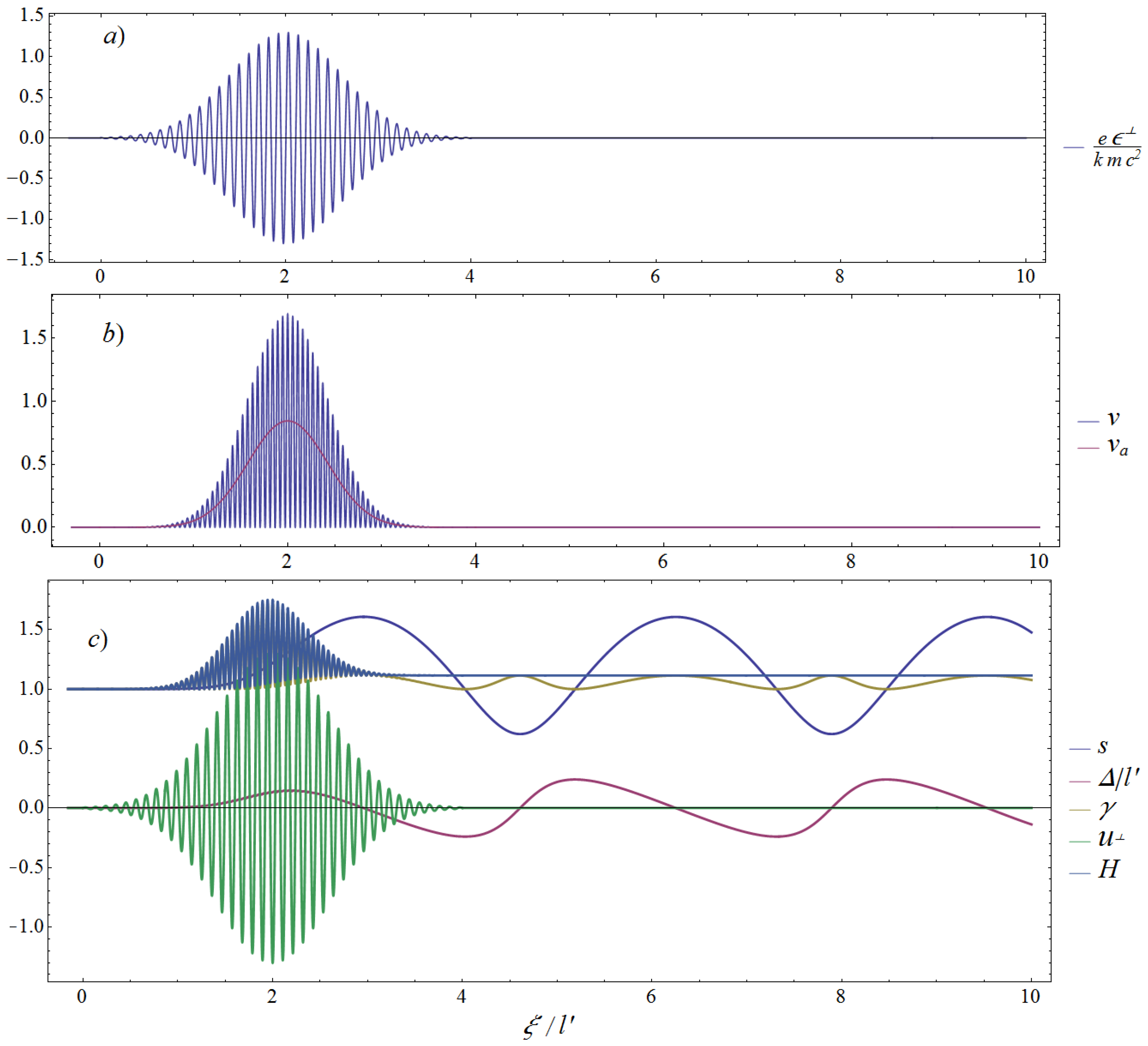
where ; once (14) is solved, we can obtain from . In Figure 1, we plot an example of a monochromatic laser pulse slowly modulated by a Gaussian along with the corresponding solution in a constant density plasma; the qualitative behaviour of the solution remains the same if const. In the NR regime , whence , , where ; at lowest order in (8) and (9) reduce to the equations , of a forced NR harmonic oscillator with trivial initial conditions. The solution is
By (8 Right), the zeroes of are extrema of and vice versa, because grows with Z. Let us recall how start evolving from their initial values (9). As previously mentioned, for all electrons reached by the pulse start to oscillate transversely and drift forward; in fact, becomes positive, implying in turn that the right-hand side (rhs) of (8 Left) and does as well; the electrons leave a layer of ions of finite thickness behind themselves that is completely evacuated of electrons. If the density vanished (), then we would obtain
grows with and is almost constant for if for (which occurs if the pulse is slowly modulated (58)). On the contrary, as the density is positive, the growth of implies the growth of the rhs of (8 Right), because the latter grows with , as well as of . Meanwhile, continues to grow as long as , and reaches a maximum at the smallest such that the rhs (8 Left) vanishes. keeps growing as long as , reaches a maximum at the first zero of , and decreases for , while is negative. reaches a negative minimum at the smallest , such that the rhs (8 Left) vanishes again. Here, we denote by the smallest such that and . We encourage the reader to single out for the solution considered in Figure 1 from the graphs in 1c. If is slowly modulated, then (see Appendix A.2 for details, and Appendix 5.4 in [31] for further information); then, if .
Definition 1.
A pulse is strictly short, essentially short with respect toif it respectively fulfills
In the NR regime, if const, these respectively amount to requiring that the corresponding solution (15) fulfills , ; if const, it is sufficient to replace with to obtain sufficient conditions for the fulfillment of (16), said conditions being
Proposition 1.
The proof is provided in Appendix A.1. The assumption that be symmetric is satisfied with very good approximation if the pulse is a slowly modulated one (58) with a symmetric modulation about (as in Figure 1b), per (59).
The following estimates hold for . First, and (13 Left) imply the bound
2.1. Constant Density Case
If , for we find by (18) , i.e.,
As grows strictly with and is convex, Equation (19) and (13 Left) in turn imply
It is apparent that vanishes at and grows with for small until its (unique) maximum point, while for larger it decreases and becomes negative. Hence, a lower bound for is the smallest such that . Therefore, ensures that .
Equation (13 Right) implies that , namely,
At least for small , this is a more stringent lower bound for s in than ; vanishes at , and grows with for small until its (unique) maximum point; for larger , it decreases and becomes negative. Hence, a lower bound for is the smallest such that . Therefore, ensures that .
2.2. Generic Density Case
Let , , be some upper, lower bounds on
for . If , then , and we can set . In general, a Z-independent choice of is ; see (4). More accurately, with such that
then for all (by the definition of ), and (22) holds, choosing
in general, (24 Left) is a lower (and therefore better) upper bound than . Henceforth we abbreviate , . By (18), we can adopt the simple choice (if , as occurs if the pulse is a slowly modulated one (58), then if , and (22) holds with for all even if ).
Lemma 1.
Proof.
For , the inequality is proven as follows:
using ; for brevity, we have not displayed the Z argument here. The inequality holds in as well, because there decreases, whereas grows. □
The maximum of in is in because in and in . To obtain upper, lower bounds for and a lower bound for in the longer interval , we use (25) to majorize
(again, if , as occurs if the pulse is a slowly modulated one (58), then if , and these results remain valid if we replace by , even if ).
When replaced in (11), this yields and , whence
where is the negative solution of the equation (as a first estimate, ). Clearly, .
Proposition 2.
For all, the dynamical variablesare bounded as follows:
where, and
whereis the zero ofas well as the maximum point of, and. Moreover, the value of the Hamiltonian is bounded by
where, dubbing the maximum ofby, we have defined
Proof.
The left inequality in (27 Left) is the already proven (18). Equation (13) by (24), (18) implies , which together with (26 Left) implies the left inequality in (27 Right); the latter, together with (13 Left), (26 Right), in turn implies the right inequality in (27 Left). First, vanishes at , grows with for small until it reaches a maximum for sufficiently large , then decreases to negative values. Hence, , i.e., the smallest such that , is indeed a lower bound for ; meanwhile, is the maximum point of f and . Equation (13) implies that for all
If , integrating (8 Right) over and recalling that there, we find
where the first inequality in the last line holds because if ; as s has its maximum in , (31) implies in particular that , which when replaced in (32) provides
the latter inequality and (31) amount to the right inequality in (27 Right), which holds, together with . The right inequality in (29) follows from (11) and (25). From , it follows for that
where again, for brevity, we have not displayed the Z argument. As the rhs has its maximum in , whereas can grow in , we obtain
If , then in , and
where the last inequality holds because in ; by summing this inequality and we obtain , which actually holds for all by (33) and because the second term is negative if . Summing up, we find in all the interval ; this, together with (11), implies the left inequality (29). □
As mentioned previously, vanishes at , grows up to its unique positive maximum at , then decreases to negative values; is the unique such that . Hence, is a lower bound for . Therefore, the condition
ensures that , namely, that the pulse is strictly short. Similarly, vanishes at , grows up to its unique positive positive maximum at , then decreases to negative values. Hence, a lower bound for is the unique such that , and the condition
ensures that , namely, that the pulse is essentially short. Moreover, with this assumption we find by (29) the following upper and lower bounds on the final Z-electron energy after their interaction with the pulse:
In Figure 3 and Figure 4, we plot for two values of Z and the associated upper and lower bounds corresponding to the densities of Figure 2, which have the same asymptotic value . As can be seen, the bounds agree well. Moreover, a useful lower bound for is provided by the following lemma.
Lemma 2.
Proof.
As a consequence, if the square bracket at the rhs (38) is nonnegative, then is as well , and therefore another condition ensuring that (i.e., that the pulse is strictly short) is
which is more easily computable, although more difficult to satisfy, than (35).
More stringent (though less easily computable) bounds than (27) could be found by replacing them in (13) and reiterating the previous arguments. The first step is the new bound , the second is setting instead of in (24), etc. However, for the scope of the present work we content ourselves with these basic relations.
3. Bounds on the Jacobian for Small
Differentiating (8), we find that the dimensionless variables
fulfill the Cauchy problem
where we have abbreviated . From , we can immediately obtain via
which is dimensionless, as well. To bound for small , we introduce the Liapunov function
where is specified below. Clearly, . Equation (42) implies
and as , , we obtain
where we have abbreviated and introduced some such that . Per the comparison principle [38], , where is the solution of the Cauchy problem , which implies
and . As grows with , if then no WBDLPI may involve the Z-electrons. Choosing , we find for all
In the NR regime, which is characterized by , we have , , , ; setting leads by a straightforward computation to
As grows with and reaches the value 1 for , we therefore find that the condition
is sufficient to ensure that the Z-electrons are not involved in WBDLPI. This is automatically satisfied if , because by definition ; otherwise, it is a very mild condition on the relative variation of the initial electron density across an interval of length and in fact to violate (48) one needs a discontinuous (or a continuous and very steep) with large relative variations around Z; see Section 4.
We now consider the general case. In the interval , the inequalities imply
where are the maxima of . Hence, we obtain the bounds
which are replaced in (46) by choosing , respectively implying
Here, we have redisplayed the Z-argument; is the most difficult to compute, while is the easiest. We thus arrive at
Theorem 1.
Assume that condition (36) is fulfilled. Then, no WBDLPI involves the Z-electrons if in addition , or at least , or at least . If one of these conditions is fulfilled for all Z, then WBDLPI occurs nowhere.
Consequently, for any fixed pump there is no WBDLPI if is sufficiently small. A simple sufficient condition is provided by the following corollary.
Corollary 1.
4. Discussion and Conclusions
As we have seen, if inequality (35) is fulfilled, then , i.e., the pulse is strictly short (that is, it completely overcomes the Z-electrons while their longitudinal displacement remains nonnegative). If at least inequality (36) is fulfilled, then , andt the pulse is essentially short (that is, the pulse completely overcomes the Z-electrons before their longitudinal displacement reaches its first negative minimum), and the inequalities (27), (29), (50) and (52) apply. If in addition one of the conditions of Proposition 1 is satisfied, then WBDLPI can be excluded.
As seen above, the more easily computable (although more difficult to satisfy) condition (40) implies (35) and the inequality , which after substitution in (50) and (52) simplifies the computation of their rhs; in particular, (52) becomes
Therefore, (40) and provide a sufficient condition to exclude WBDLPI as well.
Note that in the above conditions, several dimensionless numbers characterizing the input data, viz. , and possibly , play a key role in the main inequalities of the present paper. Therefore, their computation represents the first step in checking whether and where such conditions are fulfilled or violated.
In the NR regime (48) is equivalent to either inequality
(In fact, inequality (48) amounts to , i.e., (54); taking the square one obtains the equivalent inequality , which is fulfilled if , where solve the equation in the unknown x; the left inequality is automatically satisfied because . Dividing the inequality by p, we obtain (54)).
If grows in , then does as well, and for all the previous conditions become
This is fulfilled if, e.g., in is continuous (without excluding ), at least piecewise , and for all and .
Now, we impose that is continuous in and reaches a given value at while respecting (55). We compare the minimum for a linear and a quadratic ; note that for the former violates the above bound at . We find
where is the Heavisde step function. In fact, if , then (55 Right) becomes for all Z; the rhs is lowest for , whereby the inequality becomes (56 Right), as claimed. If , then (55 Left) becomes the condition
this is of first degree in Z, and is hence fulfilled for all if it is for . The quadratic polynomial in is positive if , as claimed, because is the positive solution of the equation in the unknown z, and automatically makes .
If is considerably larger than 1, then is considerably larger than ; in particular, assuming (2) with , i.e., , yields , . Therefore, choosing , we can exclude WBDLPI by adopting , but not . Such a result is relevant for LWFA experiments, which usually fulfill (2). From the physical viewpoint, it allows us to exclude WBDLPI because: (i) the density obtained just outside the nozzle of a supersonic gas jet (orthogonal to the ) typically is , with (see, e.g., Figure 2 in [39] or Figure 5 in [40]), and therefore is closer to type than to type ; and (ii) by causality, the effects of a pulse with a finite spot radius R near its symmetry axis are the same as with a plane wave (), at least for small . From the viewpoint of mathematical modeling, this suggests that it makes a major difference whether we describe the edge of the plasma by or by ; in the first case, we can correctly predict the plasma evolution only by kinetic theory and PIC codes, while in the second we can do this by a hydrodynamic description and less computationally demanding multifluid codes.
If we allow a discontinuous (in ) linear Ansatz (), then (55) is fulfilled if , which is again smaller than .
Although our results apply to all with support contained in , regardless of their Fourier analysis, in most applications one deals with a modulated monochromatic wave
where , . The elliptic polarization in (58) is ruled by ; it reduces to a linear one in the direction of if , to a circular one if and . If, as follows from (1), ( is the wavelength), i.e., the plasma is underdense, then the relative variations of (and ) in a -interval of length are much smaller than those of , and those of even smaller; in fact, as , , the integral in (13 Left) averages the fast variations of v to yield much smaller relative variations of , and the first integral in (13 Right) averages the residual small variations of to yield an essentially smooth (see, e.g., Figure 1). On the contrary, varies fast, as . Under rather general assumptions (see Appendix 5.2) [31],
where , and similarly for other integrals with modulated integrands. In the appendix, we recall upper bounds for the remainders . If (slow modulations); the right estimate is very good, and v can be approximated very well by . For the reasons mentioned above, replacing v by its (approximated) average over a cycle,
has only a small effect on and almost no effect on s, V, and similarly on the functions introduced in Section 2 and Section 3 to bound ; however, it simplifies their computation a great deal. As a consequence, the bounds (27), (29) and (37), as well as the short pulse conditions (35) and (36) and the no-WB conditions of proposition 1, remain essentially valid if in computing the bounds we replace v with .
We illustrate the results obtained thus far considering a pulse (58) with a linear polarization (e.g., ) and a modulation of Gaussian type, except that it is cut off outside of support :
where is the full width at half maximum of the intensity I of the electromagnetic (EM) field. More precisely, we adopt the pulse plotted in Figure 1a, which has its maximum at and ; this yields a moderately relativistic electron dynamics and . In Figure 1b, we plot the associated v and . We performed all computations and plots running our specifically designed programs using an “off the shelf” general-purpose numerical package on a common notebook for an elapsed time bewteen several seconds and several minutes. Here, we compare the impact of such a pulse on the density profiles plotted in Figure 2.
The upper bound plays the role of asymptotic value. Here, we choose cm, which is the same as the of Figure 1, which yields ; however, the results for the dimensionless variables remain the same if we change while keeping and constant. As already stated, in the case of the step-shaped density 0), if , i.e., if the pulse is strictly short (a sufficient condition for which is (35)), then , , and by (50) and (52) there is no WBDLPI; more directly, this is a consequence of for , which follows from the Z-independence of in such an interval. As for the other profiles, we have respectively plotted the following:
- In Figure 7 and Figure 8, the corresponding worldlines of the Z-electrons for and , associated with the initial electron density profiles (3) and (4). The support of the EM pulse is coloured pink (the red part is the more intense part); the laser–plasma interaction takes place in the spacetime region which has nonempty intersection with worldlines of electrons or protons.
We compare the results for densities (1)–(2) and those for densities (3)–(4) side by side. In case (1), WBDLPI is avoided assuming that , although worldlines intersect and WB takes place not far from the laser–plasma interaction region. In case (2), WBDLPI takes place for due to the steep growth of from the value . In case (3), although the growth is much less steep, again worldlines intersect and WB takes place not very far from the laser–plasma interaction region. Finally, in case (4) this occurs quite far from the latter, consistently with the results , . Thus, we note that although such dynamics are moderately relativistic rather than nonrelativistic, switching from profile (1) to profile (2) or from profile (3) to profile (4) has the same qualitative effect of avoiding (or distancing from) WBDLPI. We additionally note that in cases (1) and (3) the worldlines first intersect with very small angles, or equivalently that when the corresponding electrons collide their longitudinal momenta differ by only a very small amount. By Formula (43), is very small both because is as well and because and . Hence, we can expect that these collisions will lead only to very small momentum spreading.
Essentially the same results are reached when choosing a different pulse polarization, because is of the same type. In the case of circular polarization (, ) and Gaussian modulation v, it will itself essentially coincide with , thus displaying a single maximum (see Figure 1b).
As mentioned in the introduction, the equations of motion for the Z-electrons can be reduced to the form (8), and thus are decoupled from those of all -electrons, , only in the idealization where the laser pulse is “undepleted”, i.e., not affected by its interaction with the plasma. The latter is expected to be an acceptable approximation only for small . Actually, for a slowly modulated monochromatic wave we can show by self-consistency [28] that this is a good approximation in the spacetime region that is the intersection of the ‘laser–plasma interaction’ stripe with the orthogonal stripe
In view of the inequalities and (1) or (16), we can see that, to our satisfaction, this region is much longer than l in the direction. Thus, if cm and the pulse is as in Figure 1, we can consider the latter as undepleted and the electrons’ motion determined above as accurate for time intervals , where is at least a few s.
The above predictions are based on idealizing the initial laser pulse as a plane EM wave (5). In a more realistic picture, the laser pulse is cylindrically symmetric around the -axis and has a finite spot radius R, namely, the EM fields are of the form , where , while is 1 for and rapidly approaches zero for . By causality, the motion of the electrons remains [25] strictly the same in the future Cauchy development of , where and , and almost the same in a neighbourhood of ; therefore, the conditions described above remain sufficient to exclude WBDLPI at least in such a region. (Recall that the future Cauchy development of a region in Minkowski spacetime is defined as the set of all points for which every past-directed causal, i.e., non-spacelike, line through x intersects .)
Finally, the conditions of Proposition 1 are very general in that they apply to discontinuous or non-monotone ; however, if has a bounded derivative, it turns out that they are unnecessarily too strong for ensuring that no WBDLPI occurs. Weaker no-WBDLPI conditions under the latter assumptions are treated in [28].
Author Contributions
Conceptualization, G.F., R.F. and D.J.; Formal analysis, G.F.; Investigation, G.F.; Methodology, M.D.A. and G.G.; Validation, D.J.; Visualization, G.F.; Writing, original draft, G.F.; Writing, review and editing, M.D.A., R.F., G.G. and D.J. All authors have read and agreed to the published version of the manuscript.
Funding
This research received no external funding.
Institutional Review Board Statement
Not applicable.
Informed Consent Statement
Not applicable.
Data Availability Statement
Not applicable.
Conflicts of Interest
The authors declare no conflict of interest.
Appendix A
Appendix A.1. Proof of Proposition 1
If , both integrands in (A1) are nonnegative, as are the factors of both integrals, and moreover the latter and itself are positive if and zero if . In either case, for all , because (as , ). Moreover, if is sufficiently small, then both integrals and are positive, whereas ; the second negative term will dominate and make (A1) negative as well. Therefore, (17 Left) will be satisfied iff , i.e., if .
Similarly, if , the factors of both integrals in (A2) vanish, and . If is sufficiently small, then , whereas , and the second term dominates over the first. Under our assumptions, the second integral will be negative, because is larger where . Hence, (A2) will be negative if (and is sufficiently small); if (and is sufficiently small), then (A2) will be positive, and for , because (as in this case . Therefore, (17 Right) will be satisfied iff , i.e., if .
Appendix A.2. Estimates of Oscillatory Integrals
Here, we recall useful estimates [31] of oscillatory integrals such as (6 Left) in case (58). Given a function , integrating by parts we find that for all
Hence, we find the following upper bounds for the remainder :
It follows that . All inequalities in (A5) are useful; the left inequalities are more stringent, while the right ones are -independent.
Equations (A3) and (A5) and hold if (a Sobolev space), and in particular if and , because the previous steps can be performed under such assumptions. Equations (A3) will hold with a remainder under weaker assumptions, e.g., if is bounded and piecewise continuous and , although will be a sum of contributions such as (A4) for every interval in which is continuous.
References
- Kruer, W. The Physics Of Laser Plasma Interactions; CRC Press: Boca Raton, FL, USA, 2019; 200p. [Google Scholar]
- Sprangle, P.; Esarey, E.; Ting, A. Nonlinear interaction of intense laser pulses in plasmas. Phys. Rev. 1990, A41, 4463. [Google Scholar] [CrossRef] [PubMed]
- Sprangle, P.; Esarey, E.; Ting, A. Nonlinear Theory of Intense Laser-Plasma Interactions. Phys. Rev. Lett. 1990, 64, 2011. [Google Scholar] [CrossRef] [PubMed]
- Esarey, E.; Schroeder, C.B.; Leemans, W.P. Physics of laser-driven plasma-based electron accelerators. Rev. Mod. Phys. 2009, 81, 1229. [Google Scholar] [CrossRef]
- Macchi, A. A Superintense Laser-Plasma Interaction Theory Primer; Springer: Berlin/Heidelberg, Germany, 2013. [Google Scholar]
- Kuzenov, V.V.; Ryzhkov, S.V. Numerical simulation of the effect of laser radiation on matter in an external magnetic field. J. Phys. Conf. Ser. 2017, 830, 012124. [Google Scholar] [CrossRef] [Green Version]
- Tajima, T.; Dawson, J.M. Laser Electron Accelerator. Phys. Rev. Lett. 1979, 43, 267. [Google Scholar] [CrossRef] [Green Version]
- Sprangle, P.; Esarey, E.; Ting, A.; Joyce, G. Laser wakefield acceleration and relativistic optical guiding. Appl. Phys. Lett. 1988, 53, 2146. [Google Scholar] [CrossRef]
- Tajima, T.; Nakajima, K.; Mourou, G. Laser acceleration. Riv. N. Cim. 2017, 40, 34. [Google Scholar]
- Hidding, B.; Beaton, A.; Boulton, L.; Corde, S.; Doepp, A.; Habib, F.A.; Heinemann, T.; Irman, A.; Karsch, S.; Kirwan, G.; et al. Fundamentals and Applications of Hybrid LWFA-PWFA. Appl. Sci. 2019, 9, 2626. [Google Scholar] [CrossRef] [Green Version]
- Weikum, M.K.; Akhter, T.; Alesini, P.D.; Alexandrova, A.S.; Anania, M.P.; Andreev, N.E.; Andriyash, I.; Aschikhin, A.; Assmann, R.W.; Audet, T.; et al. EuPRAXIA—A compact, cost-efficient particle and radiation source. AIP Conf. Proc. 2019, 2160, 040012. [Google Scholar]
- Weikum, M.K.; Akhter, T.; Alesini, D.; Alexandrova, A.S.; Anania, M.P.; Andreev, N.E.; Andriyash, I.A.; Aschikhin, A.; Assmann, R.W.; Audet, T.; et al. Status of the Horizon 2020 EuPRAXIA conceptual design study. J. Phys. Conf. Ser. 2019, 1350, 012059. [Google Scholar] [CrossRef]
- Assmann, R.W.; Weikum, M.K.; Akhter, T.; Alesini, D.; Alexandrova, A.S.; Anania, M.P.; Andreev, N.E.; Andriyash, I.; Artioli, M.; Aschikhin, A.; et al. EuPRAXIA Conceptual Design Report. Eur. Phys. J. Spec. Top. 2020, 229, 3675–4284, Erratum in Eur. Phys. J. Spec. Top. 2020, 229, 4285–4287. [Google Scholar] [CrossRef]
- Tomassini, P.; Nicola, S.D.; Labate, L.; Londrillo, P.; Fedele, R.; Terzani, D.; Gizzi, L.A. The resonant multi-pulse ionization injection. Phys. Plasmas 2017, 24, 103120. [Google Scholar] [CrossRef] [Green Version]
- Fiore, G.; Fedele, R.; de Angelis, U. The slingshot effect: A possible new laser-driven high energy acceleration mechanism for electrons. Phys. Plasmas 2014, 21, 113105. [Google Scholar] [CrossRef] [Green Version]
- Akhiezer, A.I.; Polovin, R.V. Theory of wave motion of an electron plasma. Sov. Phys. JETP 1956, 3, 696. [Google Scholar]
- Gorbunov, L.M.; Kirsanov, V.I. Excitation of plasma waves by an electromagnetic wave packet. Sov. Phys. JETP 1987, 66, 290. [Google Scholar]
- Rosenzweig, J.; Breizman, B.; Katsouleas, T.; Su, J. Acceleration and focusing of electrons in two-dimensional nonlinear plasma wake fields. Phys. Rev. 1991, A44, R6189. [Google Scholar] [CrossRef]
- Mora, P.; Antonsen, T.M. Electron cavitation and acceleration in the wake of an ultraintense, self-focused laser pulse. Phys. Rev. 1996, E53, R2068(R). [Google Scholar] [CrossRef]
- Pukhov, A.; Meyer-ter-Vehn, J. Laser wake field acceleration: The highly non-linear broken-wave regime. Appl. Phys. 2002, B74, 355–361. [Google Scholar] [CrossRef]
- Kostyukov, I.; Pukhov, A.; Kiselev, S. Phenomenological theory of laser-plasma interaction in ‘bubble’ regime. Phys. Plasmas 2004, 11, 5256. [Google Scholar] [CrossRef]
- Lu, W.; Huang, C.; Zhou, M.; Mori, W.; Katsouleas, T. Nonlinear theory for relativistic plasma wakefields in the blowout regime. Phys. Rev. Lett. 2006, 96, 165002. [Google Scholar] [CrossRef] [Green Version]
- Lu, W.; Huang, C.; Zhou, M.; Tzoufras, M.; Tsung, F.S.; Mori, W.B.; Katsouleas, T. A nonlinear theory for multidimensional relativistic plasma wave wakefields. Phys. Plasmas 2006, 13, 056709. [Google Scholar] [CrossRef]
- Maslov, V.I.; Svystun, O.M.; Onishchenko, I.N.; Tkachenko, V.I. Dynamics of electron bunches at the laser–plasma interaction in the bubble regime. Nucl. Instrum. Meth. Phys. Res. 2016, A829, 422. [Google Scholar] [CrossRef]
- Fiore, G.; Nicola, S.D. A simple model of the slingshot effect. Phys Rev. Acc. Beams 2016, 19, 071302. [Google Scholar] [CrossRef] [Green Version]
- Fiore, G.; Nicola, S.D. A “slingshot” laser-driven acceleration mechanism of plasma electrons. Nucl. Instrum. Meth. Phys. Res. 2016, A829, 104–108. [Google Scholar] [CrossRef] [Green Version]
- Fiore, G.; Catelan, P. On cold diluted plasmas hit by short laser pulses. Nucl. Instrum. Meth. Phys. Res. 2018, A 909, 41–45. [Google Scholar] [CrossRef]
- Fiore, G.; Akhter, T.; Nicola, S.D.; Fedele, R.; Jovanović, D. On the impact of short laser pulses on cold diluted plasmas. 2022; in preparation. [Google Scholar]
- Fiore, G. The time-dependent harmonic oscillator revisited. arXiv 2022, arXiv:2205.01781. [Google Scholar]
- Fiore, G. On plane-wave relativistic electrodynamics in plasmas and in vacuum. J. Phys. A Math. Theory 2014, 47, 225501. [Google Scholar] [CrossRef] [Green Version]
- Fiore, G. Travelling waves and a fruitful ‘time’ reparametrization in relativistic electrodynamics. J. Phys. A Math. Theory 2018, 51, 085203. [Google Scholar] [CrossRef] [Green Version]
- Fiore, G. On plane waves in Diluted Relativistic Cold Plasmas. Acta Appl. Math. 2014, 132, 261. [Google Scholar] [CrossRef] [Green Version]
- Fiore, G. On very short and intense laser-plasma interactions. Ricerche Mat. 2016, 65, 491–503. [Google Scholar] [CrossRef] [Green Version]
- Fiore, G.; Catelan, P. Travelling waves and light-front approach in relativistic electrodynamics. Ricerche Mat. 2019, 68, 341–357. [Google Scholar] [CrossRef] [Green Version]
- Fiore, G. Light-front approach to relativistic electrodynamics. J. Phys. Conf. Ser. 2021, 1730, 012106. [Google Scholar] [CrossRef]
- Dawson, J.D. Nonlinear electron oscillations in a cold plasma. Phys. Rev. 1959, 113, 383. [Google Scholar] [CrossRef]
- Jovanovic, D.; Fedele, R.; Belic, M.; Nicola, S.D. Adiabatic Vlasov theory of ultrastrong femtosecond laser pulse propagation in plasma. The scaling of ultrarelativistic quasi-stationary states: Spikes, peakons, and bubbles. Phys. Plasmas 2019, 26, 123104. [Google Scholar] [CrossRef]
- Yoshizawa, T. Stability Theory by Liapunov’s Second Method; Mathematical Society of Japan: Tokyo, Japan, 1966; 223p. [Google Scholar]
- Hosokai, T.; Kinoshita, K.; Watanabe, T.; Yoshii, K.; Ueda, T.; Zhidokov, A.; Uesaka, M. Supersonic gas jet target for generation of relativistic electrons with 12-TW 50-fs laser pulse. In Proceedings of the 8th European Conference, EPAC 2002, Paris, France, 3–7 June 2002; pp. 981–983. [Google Scholar]
- Veisz, L.; Buck, A.; Nicolai, M.; Schmid, K.; Sears, C.M.S.; Sävert, A.; Mikhailova, J.M.; Krausz, F.; Kaluza, M.C. Complete characterization of laser wakefield acceleration. In Proceedings of the Volume 8079, Laser Acceleration of Electrons, Protons, and Ions; and Medical Applications of Laser-Generated Secondary Sources of Radiation and Particles, Prague, Czech Republic, 18–21 April 2011. [Google Scholar]
Figure 1.
(a) Normalized amplitude of a linearly polarized (i.e., set in (58)) monochromatic laser pulse slowly modulated by a Gaussian with full width at half maximum and peak amplitude ; this yields a moderately relativistic electron dynamics, and . If m (corresponding to a pulse duration of s), and the wavelength is m, then the corresponding peak intensity must be W/cm; these are typical values obtainable by Ti:Sapphire lasers in LWFA experiments. (b) The corresponding forcing term and average-over-cycle (60) of the latter. (c) Corresponding solution of (8) and (9), or equivalently of (14) if ; this value is obtained if m and cm (a typical value of the electron density used in LWFA experiments). As expected, s is insensitive to the rapid oscillations of for , while for the energy H is conserved and the solution is periodic. The length l is determined on physical grounds; if, e.g., the plasma is created locally by the impact of the pulse itself on a gas (e.g., hydrogen or helium), then has to contain all points where the pulse intensity is sufficient to ionize the gas. Here, for simplicity and following convention, we have fixed it to be ; the possible inaccuracy of such a cut is very small, because is times the maximum of the modulation, i.e., practically zero, which makes .

Figure 2.
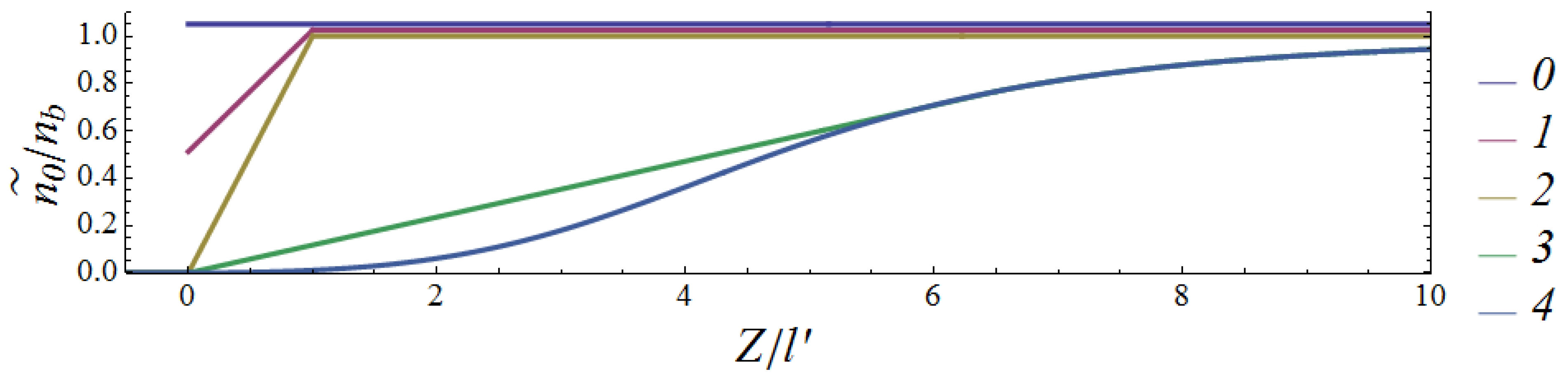
Plots of the ratios for the following initial densities: (0) . (1) . (2) . (3) , where and ; this grows as z for and coincides with the next one for . (4) .
Figure 2.
Plots of the ratios for the following initial densities: (0) . (1) . (2) . (3) , where and ; this grows as z for and coincides with the next one for . (4) .

Figure 3.
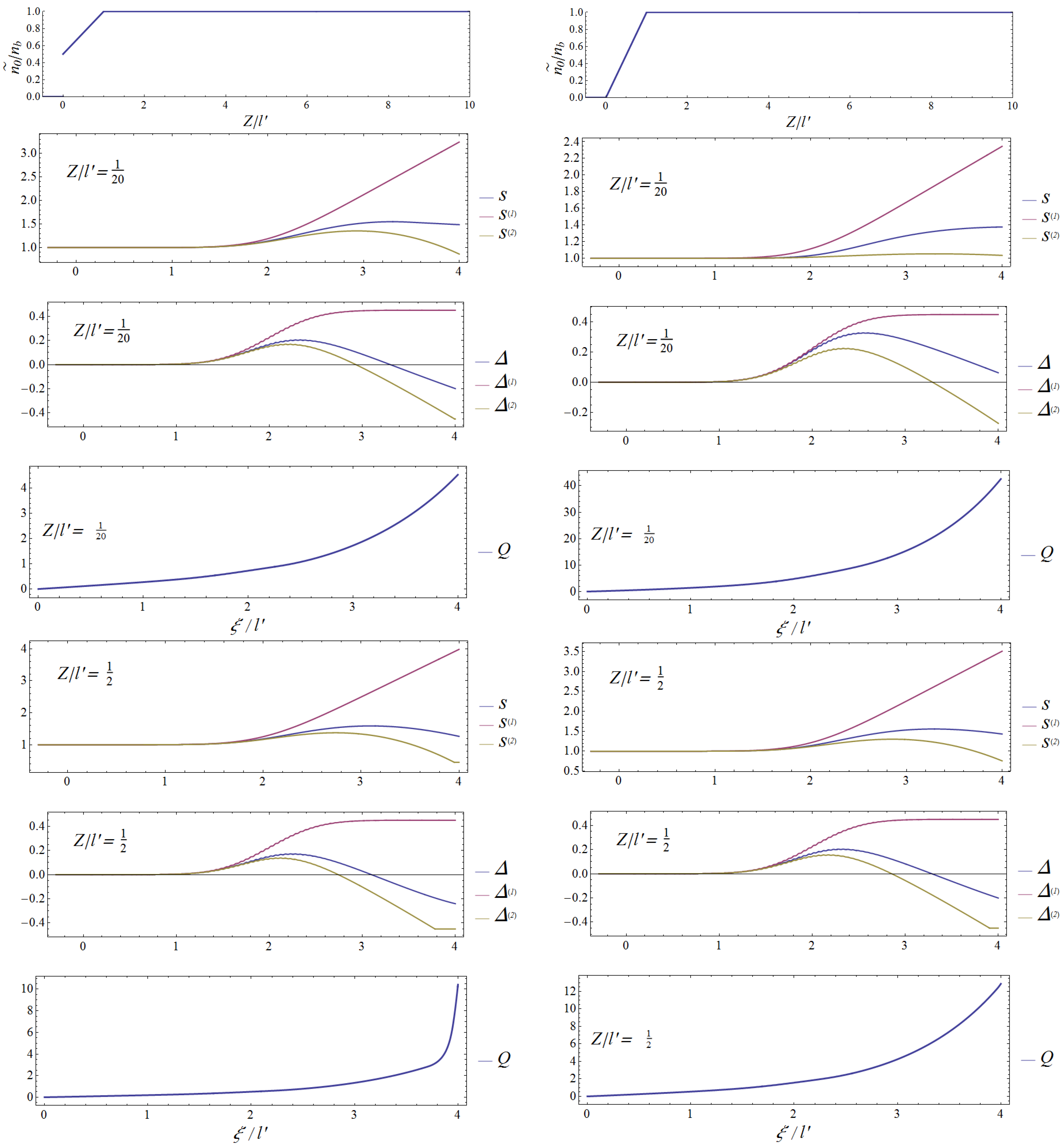
The initial electron densities (1), (2) of Figure 2 (first line; left and right, respectively). Below, assuming cm, we plot the corresponding , their upper and lower bounds , and the function Q, vs. during interaction with the pulse in Figure 1 for the same sample values, and of Z. The values can be read off the plots. As can be seen, the bounds are much better for density (1); the values are consistent with all worldlines intersecting rather far from the laser-plasma interaction spacetime region. On the other hand, the large value of for density (2) is an indication that worldlines intersect within or not far from the laser–plasma interaction spacetime region. Our computations lead to , with density (1) and , with density (2).
Figure 3.
The initial electron densities (1), (2) of Figure 2 (first line; left and right, respectively). Below, assuming cm, we plot the corresponding , their upper and lower bounds , and the function Q, vs. during interaction with the pulse in Figure 1 for the same sample values, and of Z. The values can be read off the plots. As can be seen, the bounds are much better for density (1); the values are consistent with all worldlines intersecting rather far from the laser-plasma interaction spacetime region. On the other hand, the large value of for density (2) is an indication that worldlines intersect within or not far from the laser–plasma interaction spacetime region. Our computations lead to , with density (1) and , with density (2).

Figure 4.
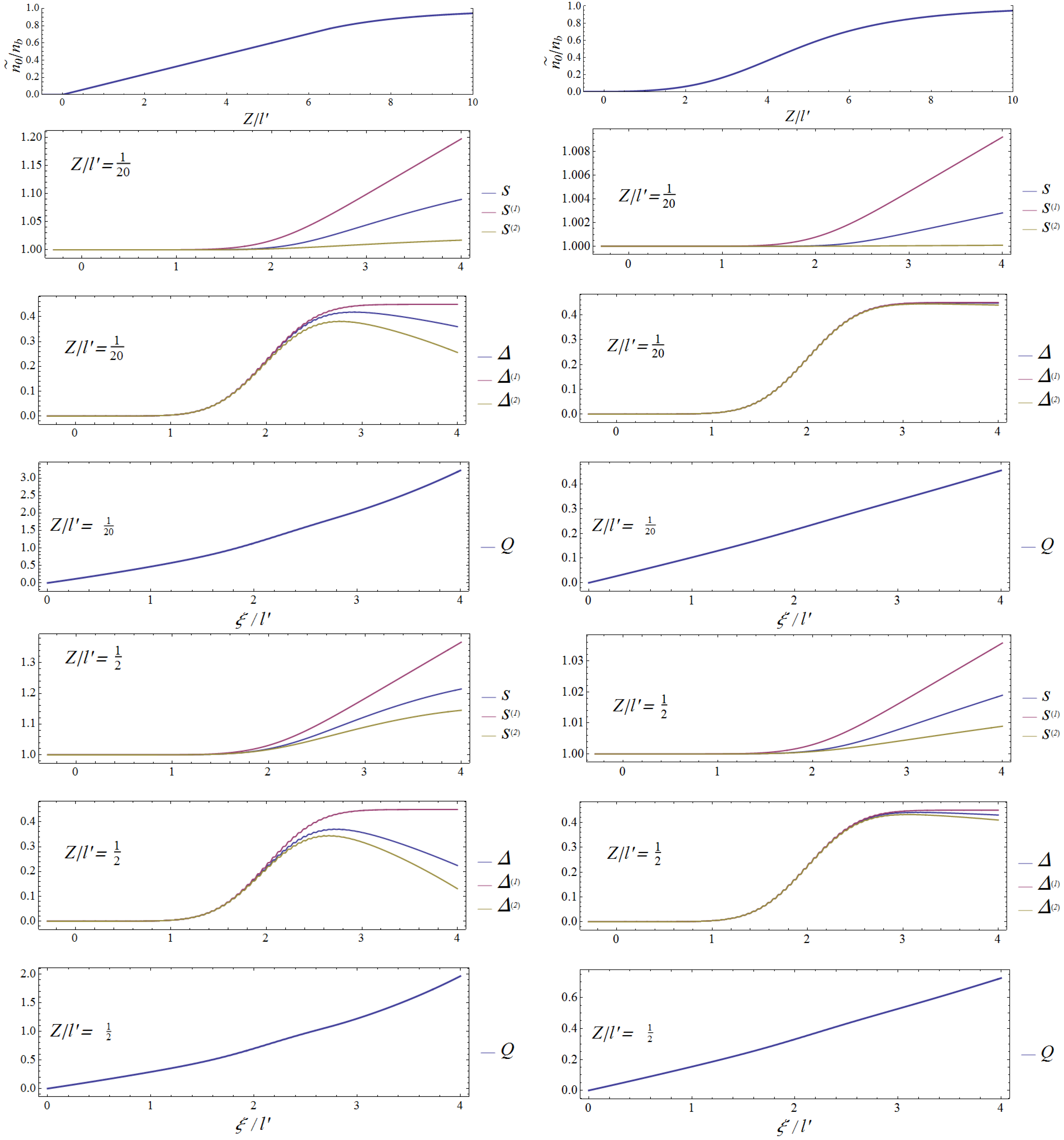
The initial electron densities (3), (4) of Figure 2 (left and right, respectively) with cm, corresponding plots of , their upper and lower bounds , and the function , vs. for the same sample values and of Z. The values can be read off the plots. As can be seen, the bounds are much better for density (4); the values are consistent with all worldlines intersecting rather far from the laser-plasma interaction spacetime region. On the other hand, the large value of for density (3) is an indication that worldlines intersect not far from the laser–plasma interaction spacetime region. Our computations lead to , with density (3) and , with density (4).
Figure 4.
The initial electron densities (3), (4) of Figure 2 (left and right, respectively) with cm, corresponding plots of , their upper and lower bounds , and the function , vs. for the same sample values and of Z. The values can be read off the plots. As can be seen, the bounds are much better for density (4); the values are consistent with all worldlines intersecting rather far from the laser-plasma interaction spacetime region. On the other hand, the large value of for density (3) is an indication that worldlines intersect not far from the laser–plasma interaction spacetime region. Our computations lead to , with density (3) and , with density (4).

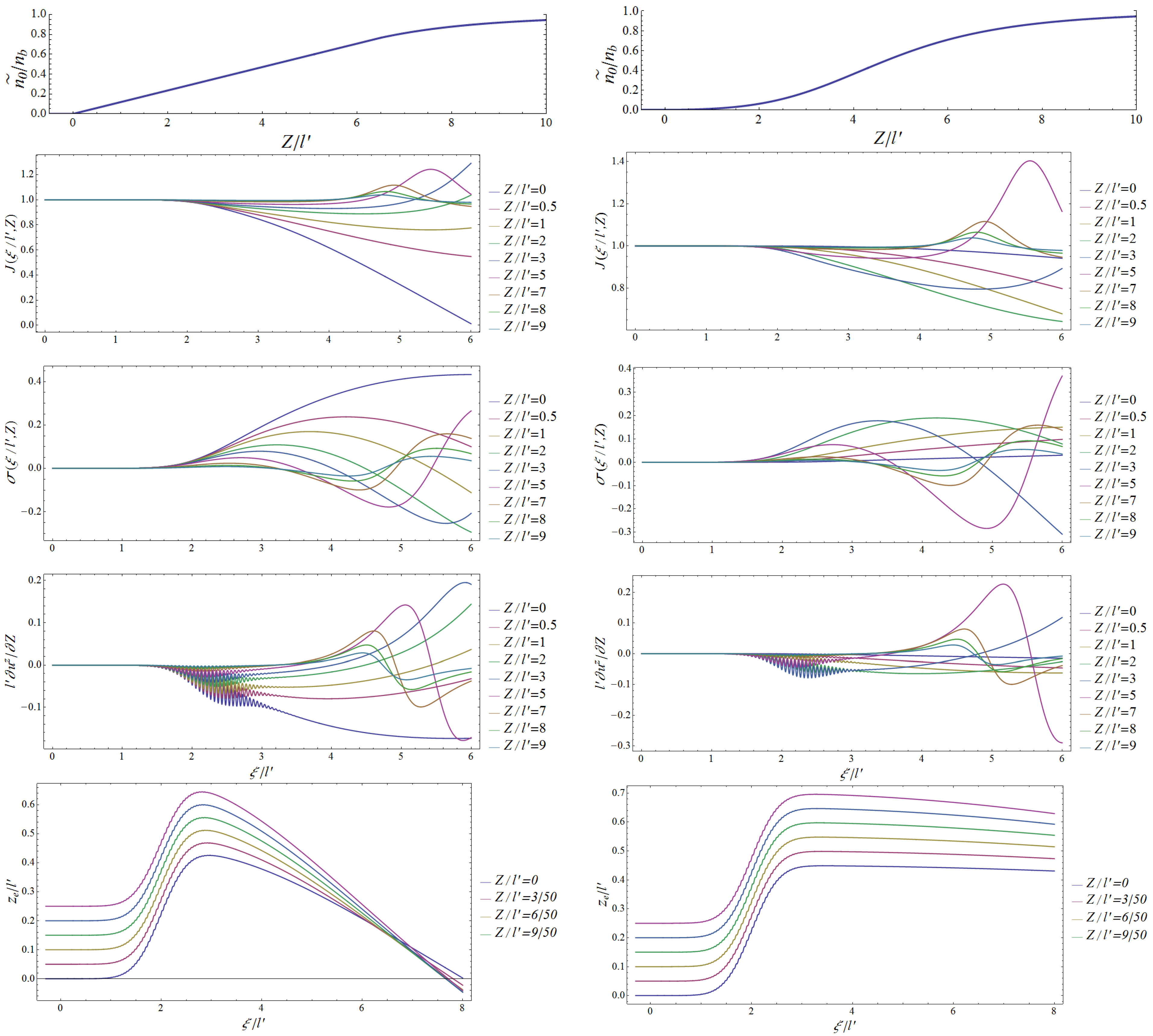
Figure 5.
The initial electron densities (3), (4) of Figure 2 (left and right, respectively) with cm, and below, the corresponding plots of during interaction with the pulse in Figure 1 for a few sample values of Z. As can be seen, J remains positive at least for all if the density is of type (4) (which grows as for ), whereas it becomes negative for and small Z if the density is of type (3) (which grows as Z for ). Correspondingly, the right-hand worldlines do not intersect, while the left-hand ones do (see the down -graphs).

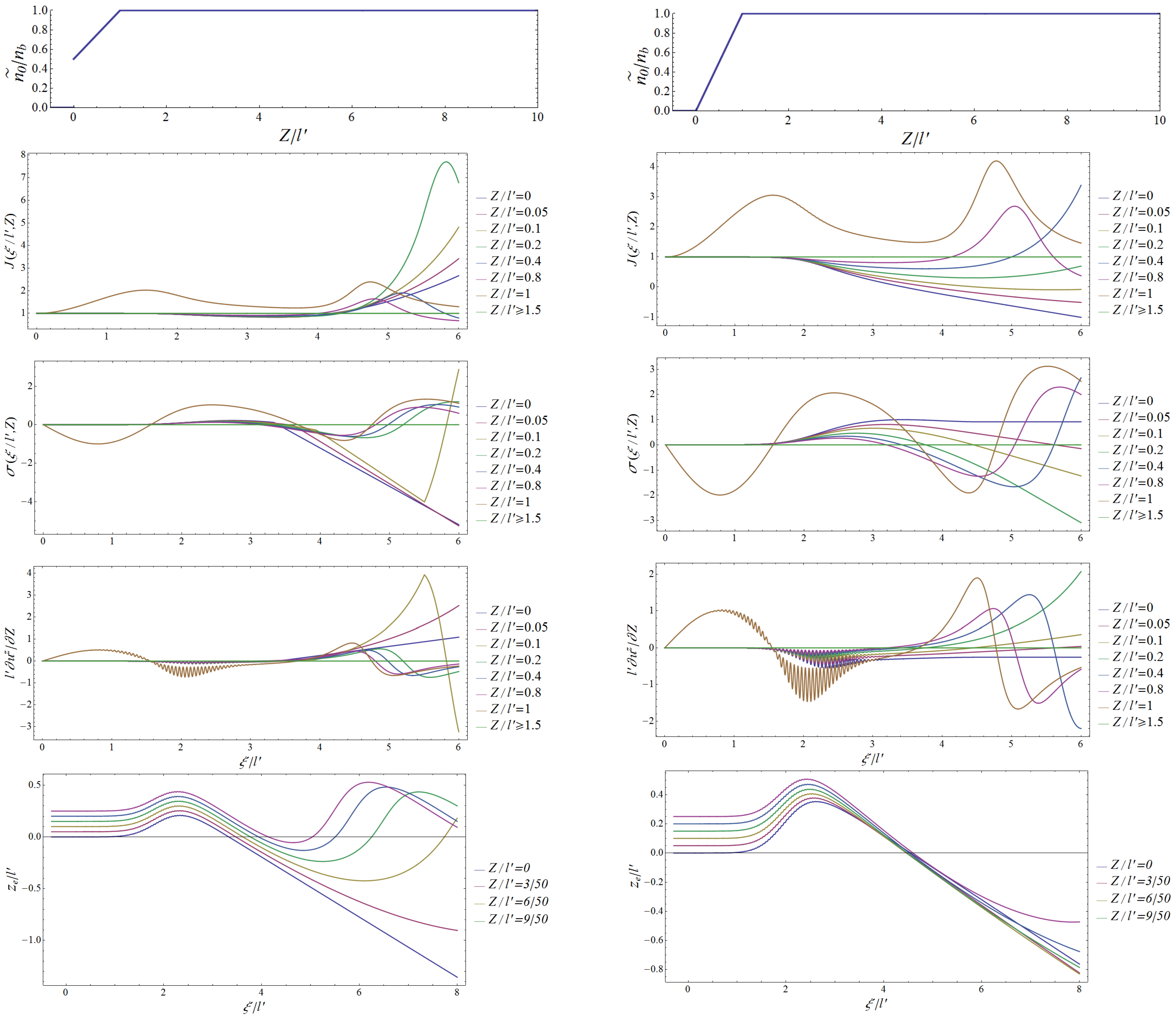
Figure 6.
The initial electron densities (1), (2) of Figure 2 (first line; respectively left, right), and below, the corresponding plots of vs. during interaction with the pulse in Figure 1 for a few sample values of Z. As can be seen, the right J remains positive for and all Z, while the left J becomes negative for very small Z and ; correspondingly, the right worldlines do not intersect, while the right ones do (see the down -graphs).

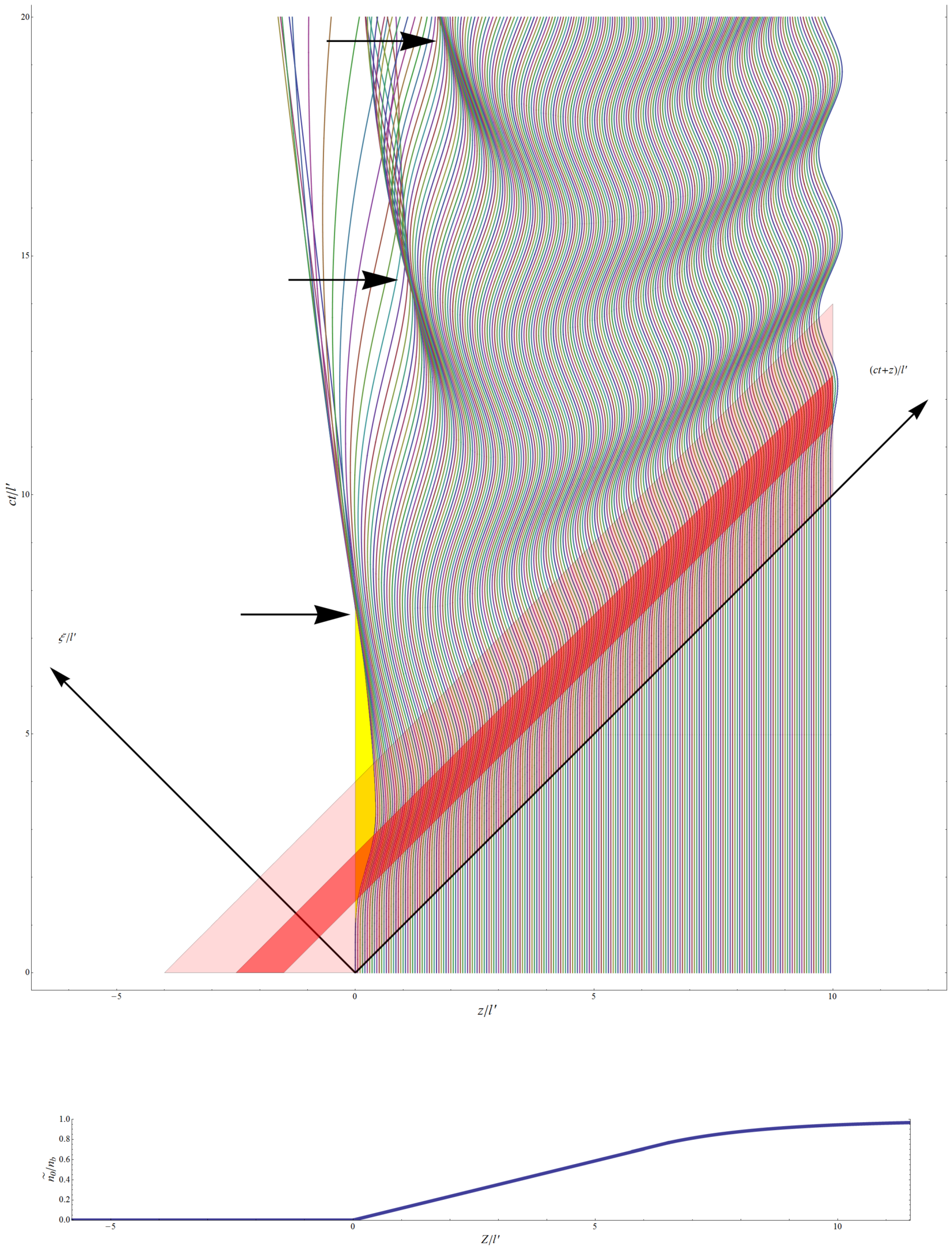
Figure 7.
Down: the initial electron density (3) of Figure 2. Up: The worldlines of Z-electrons interacting with the pulse in Figure 1 for 200 equidistant values of Z; the support and the ’effective support’ of the pulse are pink and red;, respectively, while the spacetime region of the pure-ion layer is yellow. Horizontal arrows pinpoint where particular subsets of worldlines first intersect.

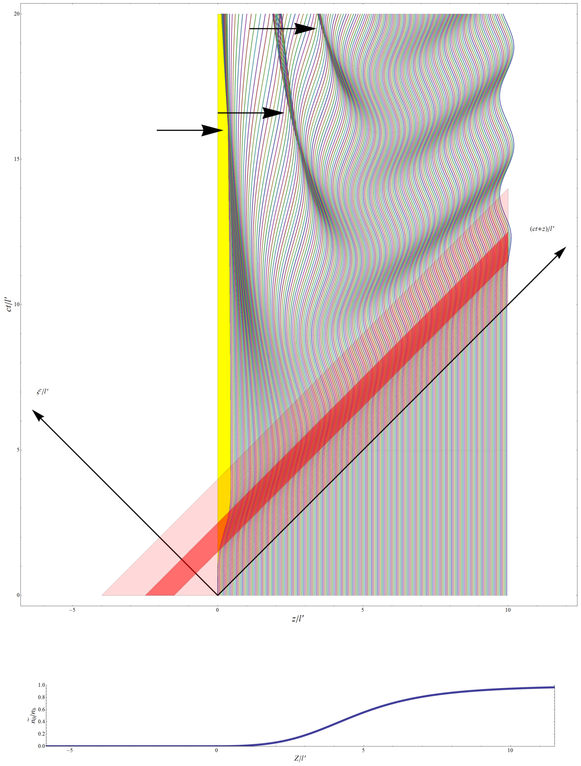
Figure 8.
Down: The initial electron density (4) of Figure 2. Up: The worldlines of Z-electrons interacting with the pulse in Figure 1 for 200 equidistant values of Z; the support and the ’effective support’ of the pulse are pink and red, respectively, while the spacetime region of the pure-ion layer is yellow. Horizontal arrows pinpoint where particular subsets of worldlines first intersect; as can be seen, small Z worldlines first intersect quite farther from the laser–plasma interaction spacetime region (shown in pink) than in the linear homogenous case (3).

Publisher’s Note: MDPI stays neutral with regard to jurisdictional claims in published maps and institutional affiliations. |
© 2022 by the authors. Licensee MDPI, Basel, Switzerland. This article is an open access article distributed under the terms and conditions of the Creative Commons Attribution (CC BY) license (https://creativecommons.org/licenses/by/4.0/).
Share and Cite
MDPI and ACS Style
Fiore, G.; De Angelis, M.; Fedele, R.; Guerriero, G.; Jovanović, D. Hydrodynamic Impacts of Short Laser Pulses on Plasmas. Mathematics 2022, 10, 2622. https://0-doi-org.brum.beds.ac.uk/10.3390/math10152622
AMA Style
Fiore G, De Angelis M, Fedele R, Guerriero G, Jovanović D. Hydrodynamic Impacts of Short Laser Pulses on Plasmas. Mathematics. 2022; 10(15):2622. https://0-doi-org.brum.beds.ac.uk/10.3390/math10152622
Chicago/Turabian StyleFiore, Gaetano, Monica De Angelis, Renato Fedele, Gabriele Guerriero, and Dušan Jovanović. 2022. "Hydrodynamic Impacts of Short Laser Pulses on Plasmas" Mathematics 10, no. 15: 2622. https://0-doi-org.brum.beds.ac.uk/10.3390/math10152622
Note that from the first issue of 2016, this journal uses article numbers instead of page numbers. See further details here.