Analysis of Stochastic M/M/c/N Inventory System with Queue-Dependent Server Activation, Multi-Threshold Stages and Optional Retrial Facility

Abstract

The purpose of this article is to examine the server activation policy (SAP) in a multi-server queuing-inventory system (MQIS). The queue has a total of c number of multi-threshold stages as well as c-homogeneous servers. The activation of each server begins one by one if there is an adequate queue length and inventory in the system; otherwise, they remain idle. The server deactivation process continues until the queue length exceeds the manageable level (predetermined stages) or there is insufficient stock. In addition, when we assume the length of the two successive threshold levels is one, the server activation policy model becomes a regular multi-server model. The Neuts matrix geometric approach is used to discuss the stability condition, stationary probability vector. The Laplace–Stieltjes transform (LST) is used to analyse the waiting time distributions of the queue and orbital customers. Additionally, significant system performance metrics and sensitivity analysis are used to investigate the effects of various parameters and cost values. In the comparative result between the server activation model (SAM) and without the server activation model (WSAM) on the expected total cost, we obtain the minimised cost in the SAM. Moreover, the results are obtained by assuming that the length of the intervals between the two successive threshold levels is to be taken into account as the non-uniform length. The expected inventory level, reorder rate, and waiting time of a customer in the waiting hall and orbit were explored numerically by the parameter analysis.

1. Introduction

The background of the paper is the practical experience of the author’s recent visit to Domino’s restaurant for a weekend celebration. When the author entered the restaurant, one of the food attendants approached him for service. Before receiving the order, he observed that two more customers had arrived simultaneously, and they were waiting for service. Immediately, the manager of the restaurant sent a new attendant to attend to them. Meanwhile, two new customers were added to their restaurant, and a new attendant was sent to take care of them. At the same time, when the number of customers in the restaurant decreases, the newly activated food attendants are directed to restock food and dining items. This process is also applicable in a textile showroom. A textile showroom recruits part-time sales executives to provide better service to customers during peak hours. This part-time recruitment helps the company to make more profit. The practical incidence encouraged the author to develop a mathematical model of the activation of the server concept in a stochastic queuing inventory system.

Most of the inventory organizations, like cafeterias, hotels, textile shops, etc., are hiring adequate part-time staff in order to provide superior service on time to the customers by applying SAP. Naturally, customers are not interested in waiting in a queue for a random time; they expect quick and better services in a short span of time. Suppose a waiting situation happens, they become impatient and will try to go to the next shop, which leads to customer loss. Getting new customers and sustaining them for a long time in business is a paramount principle of every business. In order to maintain them for a long time, the best and quickest service must be provided to them. The SAP method not only reduces customer impatience, but also reduces their waiting time and minimises the total cost.

Literature Review

Customers from a finite/infinite population stream towards a service facility in the form of a queue due to the facility’s inability to serve them all at the same time. Queues may consist of customers waiting to purchase milk and dairy products at a parlour; machines awaiting repair; trucks or vehicles awaiting service at a plant; and patients in need of treatment at a hospital. Queuing models are fundamentally relevant to service-oriented organizations because they suggest ways and means to increase service efficiency. The queueing methodology identifies the most efficient use of available manpower and other resources in order to improve service. In such a way, the service facility was introduced in QIS by Melikov [1] and Sigman [2]. Shophia Lawrence et al. [3] investigated the finite population environment with a service facility. They considered that an arriving customer gets satisfaction only after performing the service on the item. Krishnamoorthy et al. [4] provided the service for batch arrival based on the batch Markovian service process. For each completed service, the inventory decreases by one unit, irrespective of the batch size. Jeganathan et al. [5] investigated the queue dependent service facilities in a single server QIS. They assumed that the retrial customers started their retrial process only through the queue. Recently, ref. [6] et al. discussed the stock-dependent Markovian demand for a retrial queueing inventory system with a single server and multiple server vacations. Related to single server QIS, the reader may refer to the following papers [7,8,9,10,11,12,13,14].

When the queue length increases on a single server QIS, customers’ impatience will increase and lead to customer loss. However, the company’s profit is mostly dependent on its loyal customers. If they lose them, the profit falls. To avoid such a loss and reduce customer impatience, many companies have increased the number of servers. Jeganathan et al. [15] kept queue with two servers in which an arriving customer could join any queue under the Bernoulli schedule. They investigated the server interruption and the repair process for the homogeneous and heterogeneous service rates of the server. Jeganathan et al. [16] performed the two dedicated servers for the two queues in the QIS along with a flexible server. Also in [17], the two heterogeneous servers for two types of customers with delayed working vacation policies were discussed. Jeganathan et al. [18] recently investigated an integrated and interconnected stochastic queuing-inventory system with fresh, returned, and refurbished items. Through a dedicated channel, this system provides a multi-type service facility to an arriving multi-class customer.

In most of the inventory business, many companies pay attention to upgrading their service facilities in order to satisfy customers. For example, bike showrooms, textile shops, mobile showrooms, etc., all of these have a multi-server service facility. So, these are real-life situations that inspire many authors to bring out the best in stochastic modelling. Subsequently, many authors showed their interest in increasing the number of servers in the QIS. Krishnamoorthy et al. [19] used a multi-server retrial queue in the QIS. Since many papers with multi-server systems do not have an analytical solution, they presented an algorithmic approach for their multi-server QIS. Yadavalli et al. [20] proposed and discussed the multi-server concept in the finite population QIS. They assumed that an arriving customer goes into orbit whenever all the servers are busy and applied the LST to find the moment of unconditional waiting time (UWT) for a customer. Fong-Fan Wang et al. [21] analysed the priority multi-server service facilities for the finite retrial QIS. They also applied a generalized stochastic Petri net to investigate the change in parameters and heterogeneity of the service rate. The reader may refer to the mentioned papers [22,23,24,25,26,27,28,29] to learn more about the multi-server QIS in more detail.

For improving the multi-server QIS, Jeganathan et al. [30] initiated two types of multi-server service facility for sales of an item and service of an item separately. This was modelled from personal experience obtained from a bike showroom with an attached bike service facility. Even though this is one remarkable extension to the QIS, many business tycoons face a crucial problem when the queue is empty in the multi-server queues. The number of arriving customers on the system is uncertain and it varies differently during peak hours than during normal hours. For example, in textile shops, the arrival of customers increases during festival days, but on normal days the number of customer arrivals becomes very less in comparison with festival days.

Kuo-Hsiung Wang and Keng-Yuan Tai [31] investigated whether the change in server process is controlled by the predetermined queue length. Every time the queue length exceeds its level, the next server starts his work instantly. The extension of the paper [31] is done by Jain [32] who generalised the change of server process into the r number of servers depending on the queue length. Based on the threshold policy of the queue length, the number of servers starts their work. Suppose the queue length is less than the threshold level, then the recently activated server is removed from the system. They found the steady state solution by a recursive method. Feng Wei [33] proposed the active server and threshold level concepts in the discrete time multi-server queueing system. According to the set of threshold levels of the queue, Chakravarthy [34] applied the concept of adding/removing the backup servers to the single server in a Markovian arrival process.

Following such astute observations from the literature review, the activation of the server concept in the multi-server system was discussed in a few papers only, and this concept was applied only in the queueing system. To the best of our knowledge, the activation of the server in the QIS has not been proposed by any researcher till now. So, we realized that there must be a research gap in the QIS. To fill such a research gap in the QIS, we introduced the concept of SAP in a multi-server system. The activation of the number of servers is determined by the multiple threshold levels of the queue length. The remaining section of this paper is structured as follows. The model is described in Section 2. Section 3 analyses the model, while Section 4 analyses the waiting time. Section 5 gives the cost analysis and numerical illustration, while Section 6 is the conclusion.

2. Model Description

The paper mainly focuses on an MQIS with a SAP due to the queue length. The system receives an arriving customer in a finite queue, which holds a c number of multi-threshold stages, say $(R_0,R_1,R_2,\cdots ,R_{c-1})$. Initially, we assume the stage $R_0$ is always $1(R_0=1)$, then the succeeding stages vary either uniformly or non-uniformly as per the assumptions of the model. Whenever the first server finds that the queue has reached the stage $R_0$ and at least one item in the inventory, it will be activated immediately. When the queue length reaches the stage $R_1(R_1\ge 2)$ and there are a minimum of two items, then the second server is activated instantly. This activation process of the $i^{th}(i=1,2,\cdots ,c)$ server happens whenever the queue length reaches $R_{i-1}^{th}$-stage and there exist at least i-items in the inventory. This type of SAP is provided to reduce the servers’ working time.

Similarly, the $i^{th}$ server deactivation process also happens either the queue length is less than $R_{i-1}^{th}$-stage or there is no minimum stock available (${\varrho }_2<i$) in the inventory. The deactivation policy of an active server holds the discipline of the last activated server until the first idle (last activated first idle (LAFI)). If there is no customer in the queue, then all the servers are considered idle. The service process of a system begins if there is a positive queue and sufficient stock. Since the system assumes an instantaneous ordering policy, the system’s storage is never empty. At the end of the service completion of a customer, there will be one item in the inventory that is depleted correspondingly. The service rate of a customer is dependent on the number of activated servers at that time.

When the queue length reaches N, any arriving new customer may move into orbit with the probability of p or leave with its complement. The customer leaves the system when the queue size equals N is considered lost. The successful retrial process of an orbital customer goes on if the queue size is less than N. Moreover, it follows a classical retrial policy, which is defined as any one of the customers in orbit making a retrial for their service at a time dependent on the number of customers in orbit.

The arrival process of the new customer into the system follows a Poisson distribution. Exponential distribution is assumed for the two successive inter-arrival times of a retrial customer, the service process of the active servers. The arrival and service rates are introduced in the notation section. Figure 1 demonstrates the proposed model of the system.

3. Main Results

3.1. Analysis of Infinitesimal Generator Matrix

Assumption built on the birth and death process $\{(T_1\left(t\right),T_2\left(t\right),T_3\left(t\right),T_4\left(t\right)),t\ge 0\}$ forms a stochastic process and is also said to be a continuous-time Markov chain (CTMC) with a state space of D such that

$$D=\left\{({\varrho }_1,{\varrho }_2,0,0):{\varrho }_1=0,1,\cdots ;{\varrho }_2=1,\cdots ,S\right\}\cup \left(\bigcup _{j=1}^{c-1}{B}_j\right)\cup \left(\bigcup _{j=1}^{c-1}{E}_j\right)\cup Z$$

The SQIS transition matrix has the following structure, indicating the discrete state space and CTMC has follows:

$$\begin{array}{ccc}\hfill L& =& \left(\begin{array}{cccccc}{\mathbb{L}}_{00}& {\mathbb{L}}_0& \mathbf{0}& \mathbf{0}& \mathbf{0}& \cdots \\ {\mathbb{L}}_{10}& {\mathbb{L}}_{11}& {\mathbb{L}}_0& \mathbf{0}& \mathbf{0}& \cdots \\ \mathbf{0}& {\mathbb{L}}_{20}& {\mathbb{L}}_{22}& {\mathbb{L}}_0& \mathbf{0}& \cdots \\ ⋮& ⋮& ⋮& ⋮& ⋮& \ddots \end{array}\right),\hfill \end{array}$$

(1)

where

$$\begin{array}{ccc}\hfill {\mathbb{L}}_0& =& I_S\otimes p\lambda C_{N+1}.\hfill \end{array}$$

(2)

$$\begin{array}{ccc}\hfill {\mathbb{L}}_{{\varrho }_{1}0}& =& I_S\otimes {\varrho }_1\theta E_{N+1},{\varrho }_1\in 1,2,\cdots \hfill \end{array}$$

(3)

$$\begin{array}{c}\hfill \mathrm{For}{\varrho }_1=0,1,2,\cdots \\ \hfill {\left[{\mathbb{L}}_{{\varrho }_1{\varrho }_1}\right]}_{{\varrho }_2,g}& =& \left\{\begin{array}{ccc}{E}_{{\varrho }_2}\hfill & {\varrho }_2=g,\hfill & g=1,2,\cdots ,S\hfill \\ B_{{\varrho }_2}\hfill & {\varrho }_2=g+1,\hfill & g=1,2,\cdots ,S-1\hfill \\ B_{{\varrho }_2}\hfill & {\varrho }_2=1,\hfill & g=S\hfill \\ \mathbf{0},\hfill & otherwise\hfill \end{array}\right.\hfill \end{array}$$

(4)

$$\begin{array}{ccc}\hfill {\left[B_1\right]}_{1,S}& =& \left\{\begin{array}{ccc}1\mu \hfill & {\varrho }_3=1\hfill & {\varrho }_4=1\hfill \\ & {\varrho }_3^{{}^{\prime }}=0\hfill & {\varrho }_4^{{}^{\prime }}=0\hfill \\ 1\mu \hfill & {\varrho }_3=1,\hfill & {\varrho }_4={\varrho }_4^{{}^{\prime }}+1\hfill \\ & 1\le {\varrho }_3^{{}^{\prime }}=c-1\hfill & R_{{\varrho }_3^{{}^{\prime }}-1}\le {\varrho }_4^{{}^{\prime }}\le R_{{\varrho }_3^{{}^{\prime }}}-1\hfill \\ 1\mu \hfill & {\varrho }_3=1,\hfill & {\varrho }_4={\varrho }_4^{{}^{\prime }}+1\hfill \\ & {\varrho }_3^{{}^{\prime }}=c\hfill & R_{c-1}\le {\varrho }_4^{{}^{\prime }}\le N-1\hfill \\ 0,\hfill & otherwise\hfill \end{array}\right.\hfill \end{array}$$

(5)

where ${\varrho }_2=2,3,\cdots c$

$$\begin{array}{ccc}\hfill {\left[B_{{\varrho }_2}\right]}_{{\varrho }_2,{\varrho }_2-1}& =& \left\{\begin{array}{ccc}& {\varrho }_3^{{}^{\prime }}={\varrho }_3\hfill & {\varrho }_4^{{}^{\prime }}={\varrho }_4\hfill \\ {\varrho }_3\mu \hfill & 1\le {\varrho }_3\le {\varrho }_2-1,\hfill & {\varrho }_4=R_{{\varrho }_3-1}\hfill \\ & {\varrho }_3^{{}^{\prime }}={\varrho }_3-1\hfill & {\varrho }_4^{{}^{\prime }}={\varrho }_4-1\hfill \\ {\varrho }_3\mu \hfill & 1\le {\varrho }_3\le {\varrho }_2-1,\hfill & R_{{\varrho }_3-1}+1\le {\varrho }_4\le R_{{\varrho }_3}-1\hfill \\ & {\varrho }_3^{{}^{\prime }}={\varrho }_3\hfill & {\varrho }_4^{{}^{\prime }}={\varrho }_4-1\hfill \\ {\varrho }_2\mu \hfill & {\varrho }_3={\varrho }_2,\hfill & R_{{\varrho }_3-1}\le {\varrho }_4\le N\hfill \\ & {\varrho }_3^{{}^{\prime }}={\varrho }_3-1\hfill & {\varrho }_4^{{}^{\prime }}={\varrho }_4-1\hfill \\ 0,\hfill & otherwise\hfill \end{array}\right.\hfill \end{array}$$

(6)

where ${\varrho }_2=c+1,\cdots S$

$$\begin{array}{ccc}\hfill {\left[B_{{\varrho }_2}\right]}_{{\varrho }_2,{\varrho }_2-1}& =& \left\{\begin{array}{ccc}{\varrho }_3\mu \hfill & 1\le {\varrho }_3\le c-1,\hfill & {\varrho }_4=R_{{\varrho }_3-1}\hfill \\ & {\varrho }_3^{{}^{\prime }}={\varrho }_3-1\hfill & {\varrho }_4^{{}^{\prime }}={\varrho }_4-1\hfill \\ {\varrho }_3\mu \hfill & 1\le {\varrho }_3\le c-1,\hfill & R_{{\varrho }_3-1}+1\le {\varrho }_4\le R_{{\varrho }_3}-1\hfill \\ & {\varrho }_3^{{}^{\prime }}={\varrho }_3\hfill & {\varrho }_4^{{}^{\prime }}={\varrho }_4-1\hfill \\ c\mu \hfill & {\varrho }_3=c,\hfill & R_{{\varrho }_3-1}\le {\varrho }_4\le N\hfill \\ & {\varrho }_3^{{}^{\prime }}={\varrho }_3-1\hfill & {\varrho }_4^{{}^{\prime }}={\varrho }_4-1\hfill \\ 0,\hfill & otherwise\hfill \end{array}\right.\hfill \end{array}$$

(7)

where ${\varrho }_2=1,2,3,\cdots c$ and assume $R_0=1$

$$\begin{array}{ccc}\hfill {\left[E_{{\varrho }_2}\right]}_{{\varrho }_2,{\varrho }_2}& =& \left\{\begin{array}{ccc}{\overline{\delta }}_{1{\varrho }_2}\lambda \hfill & 1\le {\varrho }_3^{{}^{\prime }}\le {\varrho }_2-1,\hfill & R_{{\varrho }_3^{{}^{\prime }}-1}\le {\varrho }_4^{{}^{\prime }}\le R_{{\varrho }_3^{{}^{\prime }}}-1\hfill \\ \hfill & {\varrho }_3=({\varrho }_3^{{}^{\prime }}-1){\delta }_{(R_{{\varrho }_3^{{}^{\prime }}-1}-1){\varrho }_4}\hfill & {\varrho }_4={\varrho }_4^{{}^{\prime }}-1\hfill \\ & +{\varrho }_3^{{}^{\prime }}{\overline{\delta }}_{(R_{{\varrho }_3^{{}^{\prime }}-1}-1){\varrho }_4}\hfill & & \\ \lambda \hfill & {\varrho }_3^{{}^{\prime }}={\varrho }_2,\hfill & R_{{\varrho }_2-1}\le {\varrho }_4^{{}^{\prime }}\le N\hfill \\ & {\varrho }_3=({\varrho }_3^{{}^{\prime }}-1){\delta }_{(R_{{\varrho }_2-1}-1){\varrho }_4}\hfill & {\varrho }_4={\varrho }_4^{{}^{\prime }}-1\hfill \\ & +{\varrho }_3^{{}^{\prime }}{\overline{\delta }}_{(R_{{\varrho }_2-1}-1){\varrho }_4}\hfill & & \\ -(\lambda +{\varrho }_1\theta )\hfill & {\varrho }_3=0,\hfill & {\varrho }_4=0\hfill \\ & {\varrho }_3^{{}^{\prime }}={\varrho }_3,\hfill & {\varrho }_4^{{}^{\prime }}={\varrho }_4\hfill \\ -({\varrho }_3\mu +p\lambda )\hfill & {\varrho }_3={\varrho }_2,\hfill & {\varrho }_4=N\hfill \\ & {\varrho }_3^{{}^{\prime }}={\varrho }_3,\hfill & {\varrho }_4^{{}^{\prime }}={\varrho }_4\hfill \\ -{\overline{\delta }}_{1{\varrho }_2}(\lambda +{\varrho }_3\mu +{\varrho }_1\theta )\hfill & 1\le {\varrho }_3\le {\varrho }_2-1,\hfill & R_{{\varrho }_3-1}\le {\varrho }_4\le R_{{\varrho }_3}-1\hfill \\ & {\varrho }_3^{{}^{\prime }}={\varrho }_3\hfill & {\varrho }_4^{{}^{\prime }}={\varrho }_4\hfill \\ -(\lambda +{\varrho }_3\mu +{\varrho }_1\theta )\hfill & {\varrho }_3={\varrho }_2,\hfill & R_{{\varrho }_2-1}\le {\varrho }_4\le N-1\hfill \\ & {\varrho }_3^{{}^{\prime }}={\varrho }_3\hfill & {\varrho }_4^{{}^{\prime }}={\varrho }_4\hfill \\ 0,\hfill & otherwise.\hfill \end{array}\right.\hfill \end{array}$$

where ${\varrho }_2=c+1,c+2,c+3,\cdots S$

$$\begin{array}{ccc}\hfill {\left[E_{{\varrho }_2}\right]}_{{\varrho }_2,{\varrho }_2}& =& \left\{\begin{array}{ccc}\lambda \hfill & 1\le {\varrho }_3^{{}^{\prime }}\le c-1,\hfill & R_{{\varrho }_3^{{}^{\prime }}-1}\le {\varrho }_4^{{}^{\prime }}\le R_{{\varrho }_3^{{}^{\prime }}}-1\hfill \\ & {\varrho }_3=({\varrho }_3^{{}^{\prime }}-1){\delta }_{(R_{{\varrho }_3^{{}^{\prime }}-1}-1){\varrho }_4}\hfill & {\varrho }_4={\varrho }_4^{{}^{\prime }}-1\hfill \\ & +{\varrho }_3^{{}^{\prime }}{\overline{\delta }}_{(R_{{\varrho }_3^{{}^{\prime }}-1}-1){\varrho }_4}\hfill & & \\ \lambda \hfill & {\varrho }_3^{{}^{\prime }}={\varrho }_2,\hfill & R_{{\varrho }_2-1}\le {\varrho }_4^{{}^{\prime }}\le N\hfill \\ & {\varrho }_3=({\varrho }_3^{{}^{\prime }}-1){\delta }_{(R_{{\varrho }_2-1}-1){\varrho }_4}\hfill & {\varrho }_4={\varrho }_4^{{}^{\prime }}-1\hfill \\ & +{\varrho }_3^{{}^{\prime }}{\overline{\delta }}_{(R_{{\varrho }_2-1}-1){\varrho }_4}\hfill & & \\ -(\lambda +{\varrho }_1\theta )\hfill & {\varrho }_3=0,\hfill & {\varrho }_4=0\hfill \\ & {\varrho }_3^{{}^{\prime }}={\varrho }_3,\hfill & {\varrho }_4^{{}^{\prime }}={\varrho }_4\hfill \\ -({\varrho }_3\mu +p\lambda )\hfill & {\varrho }_3={\varrho }_2,\hfill & {\varrho }_4=N\hfill \\ & {\varrho }_3^{{}^{\prime }}={\varrho }_3,\hfill & {\varrho }_4^{{}^{\prime }}={\varrho }_4\hfill \\ -{\overline{\delta }}_{1{\varrho }_2}(\lambda +{\varrho }_3\mu +{\varrho }_1\theta )\hfill & 1\le {\varrho }_3\le c-1,\hfill & R_{{\varrho }_3-1}\le {\varrho }_4\le R_{{\varrho }_3}-1\hfill \\ & {\varrho }_3^{{}^{\prime }}={\varrho }_3\hfill & {\varrho }_4^{{}^{\prime }}={\varrho }_4\hfill \\ -(\lambda +c\mu +{\varrho }_1\theta )\hfill & {\varrho }_3=c,\hfill & R_{{\varrho }_2-1}\le {\varrho }_4\le N-1\hfill \\ & {\varrho }_3^{{}^{\prime }}={\varrho }_3\hfill & {\varrho }_4^{{}^{\prime }}={\varrho }_4\hfill \\ 0,\hfill & otherwise.\hfill \end{array}\right.\hfill \\ \hfill \end{array}$$

(8)

As we described the assumption of the model in Section 2, the following transitions produce the infinitesimal generator matrix L

• $({\varrho }_1,{\varrho }_2,{\varrho }_2,N)\stackrel{p\lambda }{\to }({\varrho }_1+1,{\varrho }_2,{\varrho }_2,N){\varrho }_1=0,1,2,\cdots ,{\varrho }_2=1,2,\cdots c$
• $({\varrho }_1,{\varrho }_2,c,N)\stackrel{p\lambda }{\to }({\varrho }_1+1,{\varrho }_2,c,N){\varrho }_1=0,1,2,\cdots ,{\varrho }_2=c+1,c+2,\cdots S$
• $({\varrho }_1,{\varrho }_2,{\varrho }_3,{\varrho }_4)\stackrel{{\varrho }_1\theta }{\to }({\varrho }_1-1,{\varrho }_2,{\varrho }_3+1,{\varrho }_4+1){\varrho }_1=1,2,\cdots ,{\varrho }_2=1,2,\cdots c,{\varrho }_3=0,1,2,\cdots {\varrho }_2-1,{\varrho }_4=R_{{\varrho }_3}-1$
• $({\varrho }_1,{\varrho }_2,{\varrho }_3,{\varrho }_4)\stackrel{{\varrho }_1\theta }{\to }({\varrho }_1-1,{\varrho }_2,{\varrho }_3,{\varrho }_4+1){\varrho }_1=1,2,\cdots ,{\varrho }_2=2,\cdots c,{\varrho }_3=1,2,\cdots {\varrho }_2-1,{\varrho }_4=R_{{\varrho }_3-1},R_{{\varrho }_3-1}+1,\cdots R_{{\varrho }_3}-2$
• $({\varrho }_1,{\varrho }_2,{\varrho }_2,{\varrho }_4)\stackrel{{\varrho }_1\theta }{\to }({\varrho }_1-1,{\varrho }_2,{\varrho }_2,{\varrho }_4+1){\varrho }_1=1,2,\cdots ,{\varrho }_2=1,2,\cdots c,{\varrho }_4=R_{{\varrho }_2-1},R_{{\varrho }_2-1}+1,\cdots N-1$
• $({\varrho }_1,{\varrho }_2,{\varrho }_3,{\varrho }_4)\stackrel{{\varrho }_1\theta }{\to }({\varrho }_1-1,{\varrho }_2,{\varrho }_3+1,{\varrho }_4+1){\varrho }_1=1,2,\cdots ,{\varrho }_2=c+1,c+2,\cdots S,{\varrho }_3=0,1,2,\cdots c-1,{\varrho }_4=R_{{\varrho }_3}-1$
• $({\varrho }_1,{\varrho }_2,{\varrho }_3,{\varrho }_4)\stackrel{{\varrho }_1\theta }{\to }({\varrho }_1-1,{\varrho }_2,{\varrho }_3,{\varrho }_4+1){\varrho }_1=1,2,\cdots ,{\varrho }_2=c+1,c+2,\cdots S,{\varrho }_3=1,2,\cdots c-1,{\varrho }_4=R_{{\varrho }_3-1},R_{{\varrho }_3-1}+1,\cdots R_{{\varrho }_3}-2$
• $({\varrho }_1,{\varrho }_2,c,{\varrho }_4)\stackrel{{\varrho }_1\theta }{\to }({\varrho }_1-1,{\varrho }_2,c,{\varrho }_4+1){\varrho }_1=1,2,\cdots ,{\varrho }_2=c+1,c+2,\cdots S,{\varrho }_4=R_{c-1},R_{c-1}+1,\cdots N-1$
• $({\varrho }_1,{\varrho }_2,{\varrho }_3,{\varrho }_4)\stackrel{\lambda }{\to }({\varrho }_1,{\varrho }_2,{\varrho }_3+1,{\varrho }_4+1){\varrho }_1=0,1,2,\cdots ,{\varrho }_2=1,2,\cdots c,{\varrho }_3=0,1,2,\cdots {\varrho }_2-1,{\varrho }_4=R_{{\varrho }_3}-1$
• $({\varrho }_1,{\varrho }_2,{\varrho }_3,{\varrho }_4)\stackrel{\lambda }{\to }({\varrho }_1,{\varrho }_2,{\varrho }_3,{\varrho }_4+1){\varrho }_1=0,1,2,\cdots ,{\varrho }_2=2,\cdots c,{\varrho }_3=1,2,\cdots {\varrho }_2-1,{\varrho }_4=R_{{\varrho }_3-1},R_{{\varrho }_3-1}+1,\cdots R_{{\varrho }_3}-2$
• $({\varrho }_1,{\varrho }_2,{\varrho }_2,{\varrho }_4)\stackrel{\lambda }{\to }({\varrho }_1,{\varrho }_2,{\varrho }_2,{\varrho }_4+1){\varrho }_1=0,1,2,\cdots ,{\varrho }_2=1,2,\cdots c,{\varrho }_4=R_{{\varrho }_2-1},R_{{\varrho }_2-1}+1,\cdots N-1$
• $({\varrho }_1,{\varrho }_2,{\varrho }_3,{\varrho }_4)\stackrel{\lambda }{\to }({\varrho }_1,{\varrho }_2,{\varrho }_3+1,{\varrho }_4+1){\varrho }_1=0,1,2,\cdots ,{\varrho }_2=c+1,c+2,\cdots S,{\varrho }_3=0,1,2,\cdots c-1,{\varrho }_4=R_{{\varrho }_3}-1$
• $({\varrho }_1,{\varrho }_2,{\varrho }_3,{\varrho }_4)\stackrel{\lambda }{\to }({\varrho }_1,{\varrho }_2,{\varrho }_3,{\varrho }_4+1){\varrho }_1=0,1,2,\cdots ,{\varrho }_2=c+1,c+2,\cdots S,{\varrho }_3=1,2,\cdots c-1,{\varrho }_4=R_{{\varrho }_3-1},R_{{\varrho }_3-1}+1,\cdots R_{{\varrho }_3}-2$
• $({\varrho }_1,{\varrho }_2,c,{\varrho }_4)\stackrel{\lambda }{\to }({\varrho }_1,{\varrho }_2,c,{\varrho }_4+1){\varrho }_1=0,1,2,\cdots ,{\varrho }_2=c+1,c+2,\cdots S,{\varrho }_4=R_{c-1},R_{c-1}+1,\cdots N-1$
• $({\varrho }_1,1,1,1)\stackrel{1\mu }{\to }({\varrho }_1,S,0,0){\varrho }_1=0,1,\cdots$
• $({\varrho }_1,1,1,{\varrho }_4+1)\stackrel{1\mu }{\to }({\varrho }_1,S,{\varrho }_3,{\varrho }_4){\varrho }_1=0,1,\cdots ,{\varrho }_3=1,\cdots c-1,{\varrho }_4=R_{{\varrho }_3-1},\cdots ,R_{{\varrho }_3}-1$
• $({\varrho }_1,1,1,{\varrho }_4+1)\stackrel{1\mu }{\to }({\varrho }_1,S,c,{\varrho }_4){\varrho }_1=0,1,\cdots ,{\varrho }_4=R_{c-1},\cdots ,N-1$
• $({\varrho }_1,{\varrho }_2,{\varrho }_3,R_{{\varrho }_3-1})\stackrel{{\varrho }_2\mu }{\to }({\varrho }_1,{\varrho }_2-1,{\varrho }_3-1,R_{{\varrho }_3-1}-1){\varrho }_1=0,1,\cdots ,{\varrho }_2=2,\cdots c,{\varrho }_3=1,\cdots {\varrho }_2-1$
• $({\varrho }_1,{\varrho }_2,{\varrho }_3,{\varrho }_4)\stackrel{{\varrho }_2\mu }{\to }({\varrho }_1,{\varrho }_2-1,{\varrho }_3,{\varrho }_4-1){\varrho }_1=0,1,\cdots ,{\varrho }_2=2,\cdots c,{\varrho }_3=1,\cdots {\varrho }_2-1,{\varrho }_4=R_{{\varrho }_3-1}+1,\cdots ,R_{{\varrho }_3}-1$
• $({\varrho }_1,{\varrho }_2,{\varrho }_3,{\varrho }_4)\stackrel{{\varrho }_2\mu }{\to }({\varrho }_1,{\varrho }_2-1,{\varrho }_3-1,{\varrho }_4-1){\varrho }_1=0,1,\cdots ,{\varrho }_2=2,\cdots c,{\varrho }_3={\varrho }_2,{\varrho }_4=R_{{\varrho }_3-1},\cdots ,N$
• $({\varrho }_1,{\varrho }_2,{\varrho }_3,R_{{\varrho }_3-1})\stackrel{{\varrho }_2\mu }{\to }({\varrho }_1,{\varrho }_2-1,{\varrho }_3-1,R_{{\varrho }_3-1}-1){\varrho }_1=0,1,\cdots ,{\varrho }_2=c+1,\cdots ,S,{\varrho }_3=1,\cdots c-1$
• $({\varrho }_1,{\varrho }_2,{\varrho }_3,{\varrho }_4)\stackrel{{\varrho }_2\mu }{\to }({\varrho }_1,{\varrho }_2-1,{\varrho }_3,{\varrho }_4-1){\varrho }_1=0,1,\cdots ,{\varrho }_2=c+1,\cdots ,S,{\varrho }_3=1,\cdots c-1,{\varrho }_4=R_{{\varrho }_3-1}+1,\cdots ,R_{{\varrho }_3}-1$
• $({\varrho }_1,{\varrho }_2,{\varrho }_3,{\varrho }_4)\stackrel{{\varrho }_2\mu }{\to }({\varrho }_1,{\varrho }_2-1,{\varrho }_3-1,{\varrho }_4-1){\varrho }_1=0,1,\cdots ,{\varrho }_2=c+1,\cdots ,S,{\varrho }_3=c,{\varrho }_4=R_{c-1},\cdots ,N$

In order to make the row sum of a infinitesimal generator matrix become zero, we apply the following transition probability.

$$p(({\varrho }_1,{\varrho }_2,{\varrho }_3,{\varrho }_4),({\varrho }_1,{\varrho }_2,{\varrho }_3,{\varrho }_4))=-\underset{({\varrho }_1^{{}^{\prime }},{\varrho }_2^{{}^{\prime }},{\varrho }_3^{{}^{\prime }},{\varrho }_4^{{}^{\prime }})\ne ({\varrho }_1,{\varrho }_2,{\varrho }_3,{\varrho }_4)}{\sum _{{\varrho }_1^{{}^{\prime }}}\sum _{{\varrho }_2^{{}^{\prime }}}\sum _{{\varrho }_3^{{}^{\prime }}}\sum _{{\varrho }_4^{{}^{\prime }}}}p(({\varrho }_1,{\varrho }_2,{\varrho }_3,{\varrho }_4),({\varrho }_1^{{}^{\prime }},{\varrho }_2^{{}^{\prime }},{\varrho }_3^{{}^{\prime }},{\varrho }_4^{{}^{\prime }}))$$

Using all the above said transitions, we obtain an infinitesimal generator matrix L as in Equation (1).

3.2. Matrix Geometric Approximation

Steady State Analysis

To perform the system characteristics of the model, we need to find the stationary probability vector, ${\Phi }$ related to the matrix L. Since the system admits classical retrial policy, there exist a some analytical difficulty on the process of finding ${\Phi }$. To overcome this problem, we apply Neuts’ matrix geometric approach based on the truncation point. The truncation point is defined as the point M, where $M\ge 1$ in which the system allows the classical retrial policy and constant retrial policy when ${\varrho }_1<M$ and ${\varrho }_1\ge M$, respectively. More explicitly, by setting ${\mathbb{L}}_{{\varrho }_{1}0}={\mathbb{L}}_{M0}$ and ${\mathbb{L}}_{{\varrho }_1{\varrho }_1}={\mathbb{L}}_{MM}$ for all ${\varrho }_1\ge M$, we determine the equilibrium for the considered system. Then, the structure of the modified L as given below:

$$\begin{array}{ccc}\hfill \widehat{L}& =& \left(\begin{array}{cccccccccccc}{\mathbb{L}}_{00}& {\mathbb{L}}_0& \mathbf{0}& \mathbf{0}& \mathbf{0}& \cdots & \mathbf{0}& \mathbf{0}& \mathbf{0}& \mathbf{0}& \mathbf{0}& \cdots \\ {\mathbb{L}}_{10}& {\mathbb{L}}_{11}& {\mathbb{L}}_0& \mathbf{0}& \mathbf{0}& \cdots & \mathbf{0}& \mathbf{0}& \mathbf{0}& \mathbf{0}& \mathbf{0}& \cdots \\ \mathbf{0}& {\mathbb{L}}_{20}& {\mathbb{L}}_{22}& {\mathbb{L}}_0& \mathbf{0}& \cdots & \mathbf{0}& \mathbf{0}& \mathbf{0}& \mathbf{0}& \mathbf{0}& \cdots \\ ⋮& ⋮& ⋮& ⋮& ⋮& \ddots & ⋮& ⋮& ⋮& ⋮& ⋮& \ddots \\ \mathbf{0}& \mathbf{0}& \mathbf{0}& \mathbf{0}& \mathbf{0}& \cdots & {\mathbb{L}}_{M0}& {\mathbb{L}}_{MM}& {\mathbb{L}}_0& \mathbf{0}& \mathbf{0}& \cdots \\ \mathbf{0}& \mathbf{0}& \mathbf{0}& \mathbf{0}& \mathbf{0}& \cdots & \mathbf{0}& {\mathbb{L}}_{M0}& {\mathbb{L}}_{MM}& {\mathbb{L}}_0& \mathbf{0}& \cdots \\ ⋮& ⋮& ⋮& ⋮& ⋮& \ddots & ⋮& ⋮& ⋮& ⋮& ⋮& \ddots \end{array}\right),\hfill \end{array}$$

Now, we shall define, ${\mathbb{L}}_M={\mathbb{L}}_{M0}+{\mathbb{L}}_{MM}+{\mathbb{L}}_0$

Theorem 1.

In order to construct the steady-state probability vector Φ associated with the generator matrix ${\mathbb{L}}_M$, where ${\mathbb{L}}_M={\mathbb{L}}_{M0}+{\mathbb{L}}_{MM}+{\mathbb{L}}_0$ is given by

$$\begin{array}{ccc}\hfill {\mathsf{\Phi }}^{\left({\varrho }_2\right)}& =& {\mathsf{\Phi }}^{\left(1\right)}{e}_{{\varrho }_2},{\varrho }_2=1,\dots ,S.\hfill \end{array}$$

(9)

where

$$\begin{array}{ccc}\hfill e_{{\varrho }_2}& =& \left\{\begin{array}{cc}I\hfill & {\varrho }_2=1\hfill \\ {(-1)}^{{\varrho }_2}{\displaystyle \prod _{j=1}^{{\varrho }_2}}{\widehat{E}}_j{\displaystyle \prod _{h=2}^{{\varrho }_2+1}}{B}_h^{-1}\hfill & {\varrho }_2=2,\cdots ,S-1\hfill \\ -B_1{\widehat{E}}_S^{-1}\hfill & {\varrho }_2=S\hfill \end{array}\right.\hfill \end{array}$$

and ${\mathsf{\Phi }}^{\left(1\right)}$ is obtained by solving ${\mathsf{\Phi }}^{\left(1\right)}[{\widehat{E}}_1-{\widehat{E}}_1{B}_2^{-1}]=\mathbf{0}$ and $\sum _{{\varrho }_2=1}^S{\mathsf{\Phi }}^{\left({\varrho }_2\right)}\mathbf{e}=1$

Proof. 

We have

$$\begin{array}{c}\hfill {\Phi }{\mathbb{L}}_M=\mathbf{0}\mathrm{and}{\Phi }\mathbf{e}=\mathbf{1}\end{array}$$

(10)

where

$$\begin{array}{ccc}\hfill {\left[{\mathbb{L}}_M\right]}_{fg}& =& \left\{\begin{array}{ccc}{\widehat{E}}_f\hfill & f=g,\hfill & g=1,2,\cdots ,S;\hfill \\ B_1\hfill & f=1,\hfill & g=S;\hfill \\ B_f\hfill & f=g+1,\hfill & g=1,2,\cdots ,S-1;\hfill \\ \mathbf{0}\hfill & otherwise\hfill \end{array}\right.\hfill \end{array}$$

The equation ${\Phi }$${\mathbb{L}}_M=$$\mathbf{0}$ yields the following set of equations:

$$\begin{array}{cc}\hfill {\mathsf{\Phi }}^{\left({\varrho }_2\right)}{\widehat{E}}_{{\varrho }_2}+{\mathsf{\Phi }}^{({\varrho }_2+1)}{B}_{{\varrho }_2+1}=\mathbf{0},& {\varrho }_2=1,\cdots ,S-1\hfill \\ \hfill {\mathsf{\Phi }}^{\left(1\right)}{B}_1+{\mathsf{\Phi }}^{\left({\varrho }_2\right)}{\widehat{E}}_{{\varrho }_2}=\mathbf{0},& {\varrho }_2=S\hfill \end{array}$$

(11)

Solving the S number of linear equations with ${\Phi }\mathbf{e}=1$, we obtained the Equation (9). □

Theorem 2.

The stability condition of $\{(T_1\left(t\right),T_2\left(t\right),T_3\left(t\right),T_4\left(t\right)),t\ge 0\}$ at M satisfies the inequality

$$r_{1}p\lambda <r_{2}M\theta$$

where$r_1={\displaystyle \sum _{{\varrho }_2=1}^c}{\mathsf{\Phi }}^{({\varrho }_2,{\varrho }_2,N)}+{\displaystyle \sum _{{\varrho }_2=c+1}^S}{\mathsf{\Phi }}^{({\varrho }_2,c,N)}$and$r_2={\displaystyle \sum _{{\varrho }_2=1}^S}{\mathsf{\Phi }}^{({\varrho }_2,0,0)}+{\displaystyle \sum _{{\varrho }_2=2}^c}{\displaystyle \sum _{{\varrho }_3=1}^{{\varrho }_2-1}}{\displaystyle \sum _{{\varrho }_4=R_{{\varrho }_3-1}}^{R_{{\varrho }_3}-1}}$

${\mathsf{\Phi }}^{({\varrho }_2,{\varrho }_3,{\varrho }_4)}+{\displaystyle \sum _{{\varrho }_2=1}^c}{\displaystyle \sum _{{\varrho }_4=R_{{\varrho }_2-1}}^{N-1}}{\mathsf{\Phi }}^{({\varrho }_2,{\varrho }_2,{\varrho }_4)}+{\displaystyle \sum _{{\varrho }_2=c+1}^S}{\displaystyle \sum _{{\varrho }_3=1}^{c-1}}{\displaystyle \sum _{{\varrho }_4=R_{{\varrho }_3-1}}^{R_{{\varrho }_3}-1}}{\mathsf{\Phi }}^{({\varrho }_2,{\varrho }_3,{\varrho }_4)}+{\displaystyle \sum _{{\varrho }_2=c+1}^S}{\displaystyle \sum _{{\varrho }_4=R_{{\varrho }_2-1}}^{N-1}}$

${\mathsf{\Phi }}^{({\varrho }_2,c,{\varrho }_4)}$.

Proof. 

When the system switches the level dependent retrial rate to a level independent retrial rate, we need to verify the inequality introduced by Neuts [35]. According to him, the considered system has the following matrix inequality

$${\mathsf{\Phi }}^{\left(M\right)}{\mathbb{L}}_0\mathbf{e}<{\mathsf{\Phi }}^{\left(M\right)}{\mathbb{L}}_{M0}\mathbf{e}.$$

To resolve the matrix inequity, the vector ${\mathsf{\Phi }}^{\left(M\right)}$ and the matrices ${\mathbb{L}}_0,{\mathbb{L}}_{M0}$ are to be exploited.

For ${\varrho }_2=1,2,\cdots ,S_1$, ${\varrho }_3=0,1,2,\cdots ,c$ and ${\varrho }_4=0,1,2,\cdots ,N.$

$${\mathsf{\Phi }}^M({\varrho }_2,{\varrho }_3,{\varrho }_4){\mathbb{L}}_0\mathbf{e}<{\mathsf{\Phi }}^L({\varrho }_2,{\varrho }_3,{\varrho }_4){\mathbb{L}}_{M0}\mathbf{e}$$

In the first step, we get

$$[{\mathsf{\Phi }}^M\left(1\right),{\mathsf{\Phi }}^M\left(2\right),\cdots ,{\mathsf{\Phi }}^M\left(S\right)]{\mathbb{L}}_0\mathbf{e}<[{\mathsf{\Phi }}^M\left(1\right),{\mathsf{\Phi }}^M\left(2\right),\cdots ,{\mathsf{\Phi }}^M\left(S\right)]{\mathbb{L}}_{M0}\mathbf{e}$$

where ${\mathsf{\Phi }}^M\left({\varrho }_2\right)={\varphi }^M({\varrho }_2,{\varrho }_3,{\varrho }_4)$

$$[{\mathsf{\Phi }}^M\left(1\right)p\lambda C_{N+1},{\mathsf{\Phi }}^M\left(2\right)p\lambda C_{N+1},\cdots ,{\mathsf{\Phi }}^M\left(S\right)p\lambda C_{N+1}]\mathbf{e}$$

$$<[{\mathsf{\Phi }}^M\left(1\right)M\theta E_{N+1},{\mathsf{\Phi }}^M\left(1\right)M\theta E_{N+1},\cdots ,{\mathsf{\Phi }}^M\left(S\right)M\theta E_{N+1}]\mathbf{e}$$

Due to the structure of $C_{N+1}$, L.H.S becomes

$${\mathsf{\Phi }}^M\left({\varrho }_2\right)p\lambda C_{N+1}={\mathsf{\Phi }}^M({\varrho }_2,{\varrho }_3,N)p\lambda .$$

On the other hand, due to structure of $E_{N+1}$ R.H.S becomes

$${\mathsf{\Phi }}^M\left({\varrho }_2\right)M\theta E_{N+1}=[{\mathsf{\Phi }}^M({\varrho }_2,{\varrho }_3,0),{\mathsf{\Phi }}^M({\varrho }_2,{\varrho }_3,1),\cdots ,{\mathsf{\Phi }}^M({\varrho }_2,{\varrho }_3,N-1)]M\theta$$

Therefore, the last inequality becomes

$$\begin{gathered} {\displaystyle \sum _{{\varrho }_2=1}^c}{\mathsf{\Phi }}^{({\varrho }_2,{\varrho }_2,N)}p\lambda +{\displaystyle \sum _{{\varrho }_2=c+1}^S}{\mathsf{\Phi }}^{({\varrho }_2,c,N)}p\lambda <{\displaystyle \sum _{{\varrho }_2=1}^S}{\mathsf{\Phi }}^{({\varrho }_2,0,0)}M\theta +{\displaystyle \sum _{{\varrho }_2=2}^c}{\displaystyle \sum _{{\varrho }_3=1}^{{\varrho }_2-1}}{\displaystyle \sum _{{\varrho }_4=R_{{\varrho }_3-1}}^{R_{{\varrho }_3}-1}}{\mathsf{\Phi }}^{({\varrho }_2,{\varrho }_3,{\varrho }_4)}M\theta + \\ {\displaystyle \sum _{{\varrho }_2=1}^c}{\displaystyle \sum _{{\varrho }_4=R_{{\varrho }_2-1}}^{N-1}}{\mathsf{\Phi }}^{({\varrho }_2,{\varrho }_2,{\varrho }_4)}M\theta +{\displaystyle \sum _{{\varrho }_2=c+1}^S}{\displaystyle \sum _{{\varrho }_3=1}^{c-1}}{\displaystyle \sum _{{\varrho }_4=R_{{\varrho }_3-1}}^{R_{{\varrho }_3}-1}}{\mathsf{\Phi }}^{({\varrho }_2,{\varrho }_3,{\varrho }_4)}M\theta +{\displaystyle \sum _{{\varrho }_2=c+1}^S}{\displaystyle \sum _{{\varrho }_4=R_{{\varrho }_2-1}}^{N-1}}{\mathsf{\Phi }}^{({\varrho }_2,c,{\varrho }_4)}M\theta \end{gathered}$$

Hence,

$$r_{1}p\lambda <r_{2}M\theta$$

where

$r_1={\displaystyle \sum _{{\varrho }_2=1}^c}{\mathsf{\Phi }}^{({\varrho }_2,{\varrho }_2,N)}+{\displaystyle \sum _{{\varrho }_2=c+1}^S}{\mathsf{\Phi }}^{({\varrho }_2,c,N)}$ and $$\begin{gathered} r_2=\sum _{{\varrho }_2=1}^S{\mathsf{\Phi }}^{({\varrho }_2,0,0)}+{\displaystyle \sum _{{\varrho }_2=2}^c}{\displaystyle \sum _{{\varrho }_3=1}^{{\varrho }_2-1}}{\displaystyle \sum _{{\varrho }_4=R_{{\varrho }_3-1}}^{R_{{\varrho }_3}-1}}{\mathsf{\Phi }}^{({\varrho }_2,{\varrho }_3,{\varrho }_4)}+ \\ {\displaystyle \sum _{{\varrho }_2=1}^c}{\displaystyle \sum _{{\varrho }_4=R_{{\varrho }_2-1}}^{N-1}}{\mathsf{\Phi }}^{({\varrho }_2,{\varrho }_2,{\varrho }_4)}+{\displaystyle \sum _{{\varrho }_2=c+1}^S}{\displaystyle \sum _{{\varrho }_3=1}^{c-1}}{\displaystyle \sum _{{\varrho }_4=R_{{\varrho }_3-1}}^{R_{{\varrho }_3}-1}}{\mathsf{\Phi }}^{({\varrho }_2,{\varrho }_3,{\varrho }_4)}+{\displaystyle \sum _{{\varrho }_2=c+1}^S}{\displaystyle \sum _{{\varrho }_4=R_{{\varrho }_2-1}}^{N-1}}{\mathsf{\Phi }}^{({\varrho }_2,c,{\varrho }_4)} \end{gathered}$$ as desired. □

Remark 1.

1. Using $r_{1}p\lambda <r_{2}M\theta$, we get,

$${\displaystyle \frac{r_{1}p\lambda }{r_{2}M\theta }}<1$$

If ${\displaystyle \frac{r_{1}p}{r_{2}M}}=m\left(say\right)$, then

$${\displaystyle \frac{\lambda }{\theta }}<{\displaystyle \frac{1}{m}}$$

2. The fascinating component with regards to the stability condition is that it is independent of μ.

3.3. Limiting Behaviour of the System

The structure of the rate matrix L and the Theorem 2 indicate that the Markov process $\{T_1\left(t\right),T_2\left(t\right),T_3\left(t\right),T_4\left(t\right),t\ge 0\}$ with state space D is regular. As a result, the limiting probability distribution

$$\begin{array}{c}\hfill {\psi }^{(u,v,w,x)}=\underset{t\to \infty }{lim}Pr\left[T_1\left(t\right)={\varrho }_1,T_2\left(t\right)={\varrho }_2,T_3\left(t\right)={\varrho }_3,T_4\left(t\right)={\varrho }_4|T_1\left(0\right),T_2\left(0\right),T_3\left(0\right),T_4\left(0\right)\right],\end{array}$$

exists and is independent of the initial state. Let $\psi =\left({\psi }^{\left(0\right)},{\psi }^{\left(1\right)},\dots \right)$ satisfies

$$\psi L=\mathbf{0},\psi \mathbf{e}=\mathbf{1}.$$

We can partition the vector ${\psi }^{\left({\varrho }_1\right)},$ as

$${\psi }^{\left({\varrho }_1\right)}=\left({\psi }^{({\varrho }_1,1)},{\psi }^{({\varrho }_1,2)},\dots ,{\psi }^{({\varrho }_1,S)}\right),{\varrho }_1\ge 0$$

$${\psi }^{({\varrho }_1,{\varrho }_2)}=\left({\psi }^{({\varrho }_1,{\varrho }_2,0)},{\psi }^{(u,v,1)},\dots ,{\psi }^{(u,v,c)}\right),{\varrho }_1\ge 0,0\le {\varrho }_2\le S$$

and

$${\psi }^{({\varrho }_1,{\varrho }_2,{\varrho }_3)}=\left({\psi }^{({\varrho }_1,{\varrho }_2,{\varrho }_3,0)},{\psi }^{(u,v,{\varrho }_3,1)},\dots ,{\psi }^{(u,v,{\varrho }_3,N)}\right),{\varrho }_1\ge 0,0\le {\varrho }_2\le S,0\le {\varrho }_3\le c$$

Theorem 3.

Utilizing the vector ψ and the specific structure of L, ℜ can be determined by

$$\begin{array}{c}\hfill {\Re }^2{\mathbb{L}}_{M0}+\Re {\mathbb{L}}_{MM}+{\mathbb{L}}_0=\mathbf{0}\end{array}$$

(12)

where ℜ is the minimal non-negative of the matrix quadratic equation and has the structure

$$\begin{array}{c}\hfill \Re =\left(\begin{array}{cccc}{\Re }_{11}& {\Re }_{12}& \cdots & {\Re }_{1S}\\ {\Re }_{21}& {\Re }_{22}& \cdots & {\Re }_{2S}\\ {\Re }_{31}& {\Re }_{32}& \cdots & {\Re }_{3S}\\ ⋮& ⋮& \ddots & ⋮\\ {\Re }_{S1}& {\Re }_{S2}& \cdots & {\Re }_{SS}\end{array}\right)\end{array}$$

(13)

where

$$\begin{array}{c}\hfill {\Re }_{{\varrho }_2{\varrho }_2^{{}^{\prime }}}=\left(\begin{array}{ccccccc}0& 0& 0& 0& 0& \cdots & 0\\ 0& 0& 0& 0& 0& \cdots & 0\\ 0& 0& 0& 0& 0& \cdots & 0\\ ⋮& ⋮& ⋮& ⋮& ⋮& \ddots & ⋮\\ a_{{\varrho }_2{\varrho }_2^{{}^{\prime }}}^0& a_{{\varrho }_2{\varrho }_2^{{}^{\prime }}}^1& a_{{\varrho }_2{\varrho }_2^{{}^{\prime }}}^2& a_{{\varrho }_2{\varrho }_2^{{}^{\prime }}}^3& a_{{\varrho }_2{\varrho }_2^{{}^{\prime }}}^4& \cdots & a_{{\varrho }_2{\varrho }_2^{{}^{\prime }}}^N\end{array}\right),{\varrho }_2,{\varrho }_2^{{}^{\prime }}\in 1,\cdots ,S.\end{array}$$

Proof. 

Before solving the quadratic system in (12), first we assume unknown rate matrix ℜ as in (13). Since the matrix ${\mathbb{L}}_0$ has S non-zero rows, rate matrix ℜ also has the same number of non-zero rows. Now, applying assumed unknown matrix ℜ in Equation (12) and simplifying them, we obtain the set of following non-linear equations in which $K_h$ denotes the diagonal elements of the corresponding matrix ${\mathbb{L}}_{MM}$ where $h=1,2,\cdots ,\frac{c(c+3)}{2}+c+(S-c)(c+2).$

$\mathrm{For}i=1,2,\cdots ,S,j=1,2,\cdots ,c-1,u=N+1$

$\mathrm{For}z=0,1,\cdots ,j,v=R_z-1$

$${\delta }_{z0}\left(\sum _{m=1}^S{a}_{im}^{u-1}{a}_{jm}^{v-1}\right)M\theta +{\delta }_{z0}{a}_{ij}^{v-1}{\lambda }_r+a_{ij}^v{K}_{\frac{j(j+3)}{2}+z-1}+a_{i(j+1)}^{v+1}(z+1)\mu =0$$

$\mathrm{For}z=1,2,\cdots ,j,v=R_{z-1},\cdots ,R_z-2$

$$\left(\sum _{m=1}^S{a}_{im}^{u-1}{a}_{jm}^{v-1}\right)M\theta +a_{ij}^{v-1}\lambda +a_{ij}^v{K}_{\frac{j(j+3)}{2}+z-1}+a_{i(j+1)}^{z+1}z\mu =0$$

$\mathrm{For}v=R_j,\cdots ,N-1$

$$\left(\sum _{m=1}^S{a}_{im}^{u-1}{a}_{jm}^{v-1}\right)M\theta +a_{ij}^{v-1}\lambda +a_{ij}^v{K}_{\frac{j(j+3)}{2}+j-1}+a_{i(j+1)}^{v+1}(j+1)\mu =0$$

$\mathrm{For}v=N$

$$\left(\sum _{m=1}^S{a}_{im}^{u-1}{a}_{jm}^{v-1}\right)M\theta +a_{ij}^{v-1}\lambda +a_{ij}^v{K}_{\frac{j(j+3)}{2}+j}+{\delta }_{ij}p\lambda =0$$

$\mathrm{For}i=1,2,\cdots ,S,j=c,c+1,\cdots ,S-1,u=N+1$$\mathrm{For}z=0,1,\cdots ,c-1,v=R_z-1$

$${\delta }_{z0}\left(\sum _{m=1}^S{a}_{im}^{u-1}{a}_{jm}^{v-1}\right)M\theta +{\delta }_{z0}{a}_{ij}^{v-1}\lambda +a_{ij}^v{K}_{\frac{c(c+3)}{2}+z-1+(j-c)(c+2)}+a_{i(j+1)}^{v+1}(z+1)\mu =0$$

$\mathrm{For}z=1,2,\cdots ,c-1,v=R_{z-1},\cdots ,R_z-2$

$$\left(\sum _{m=1}^S{a}_{im}^{u-1}{a}_{jm}^{v-1}\right)M\theta +a_{ij}^{v-1}\lambda +a_{ij}^v{K}_{\frac{c(c+3)}{2}+z-1+(j-c)(c+2)}+a_{i(j+1)}^{v+1}z\mu =0$$

$\mathrm{For}v=R_{c-1},\cdots ,N-1$

$$\left(\sum _{m=1}^S{a}_{im}^{u-1}{a}_{jm}^{v-1}\right)M\theta +a_{ij}^{v-1}\lambda +a_{ij}^v{K}_{\frac{c(c+3)}{2}+c-1+(j-c)(c+2)}+a_{i(j+1)}^{v+1}c\mu =0$$

$\mathrm{For}v=N$

$$\left(\sum _{m=1}^S{a}_{im}^{u-1}{a}_{jm}^{v-1}\right)M\theta +a_{ij}^{v-1}\lambda +a_{ij}^v{K}_{\frac{c(c+3)}{2}+c+(j-c)(c+2)}+{\delta }_{ij}p\lambda =0$$

$\mathrm{For}i=1,2,\cdots ,S,j=S,u=N+1$

$\mathrm{For}z=0,1,\cdots ,c-1,v=R_z-1$

$${\delta }_{z0}\left(\sum _{m=1}^S{a}_{im}^{u-1}{a}_{jm}^{v-1}\right)M\theta +{\delta }_{z0}{a}_{ij}^{v-1}\lambda +a_{ij}^v{K}_{\frac{c(c+3)}{2}+z-1+(j-c)(c+2)}+a_{11}^{v+1}1\mu =0$$

$\mathrm{For}z=1,2,\cdots ,c-1,v=R_{z-1},\cdots ,R_z-2$

$$\left(\sum _{m=1}^S{a}_{im}^{u-1}{a}_{jm}^{v-1}\right)M\theta +a_{ij}^{v-1}\lambda +a_{ij}^v{K}_{\frac{c(c+3)}{2}+z-1+(j-c)(c+2)}+a_{11}^{v+1}1\mu =0$$

$\mathrm{For}v=R_{c-1},\cdots ,N-1$

$$\left(\sum _{m=1}^S{a}_{im}^{u-1}{a}_{jm}^{v-1}\right)M\theta +a_{ij}^{v-1}\lambda +a_{ij}^v{K}_{\frac{c(c+3)}{2}+c-1+(j-c)(c+2)}+a_{11}^{v+1}1\mu =0$$

$\mathrm{For}v=N$

$$\left(\sum _{m=1}^S{a}_{im}^{u-1}{a}_{jm}^{v-1}\right)M\theta +a_{ij}^{v-1}\lambda +a_{ij}^v{K}_{\frac{c(c+3)}{2}+c+(j-c)(c+2)}+{\delta }_{ij}p\lambda =0$$

After solving the above such equations, one can obtain the elements of ℜ matrix. □

Theorem 4.

The stationary probability vector ψ related to the generated matrix L is determined by

$$\begin{array}{c}\hfill {\psi }^{\left(i\right)}=\left\{\begin{array}{c}\sigma Y^{\left(0\right)}\prod _{j=i}^M{\mathbb{L}}_{j0}(-{\mathbb{L}}_j),0\le i\le M-1\hfill \\ \sigma Y^{\left(0\right)}{\Re }^{(i-M)},i\ge M\hfill \end{array}\right.\end{array}$$

(14)

where ℜ is the solution of the Equation (13) and

$$\begin{array}{c}\hfill \sigma ={[1+Y^{\left(0\right)}\sum _{i=0}^{M-1}\prod _{j=i}^M{\mathbb{L}}_{j0}(-{\mathbb{L}}_j)\mathbf{e}]}^{-1}\end{array}$$

(15)

where $Y\left(0\right)$ can be computed by $Y^{\left(0\right)}{(I-\Re )}^{-1}\mathbf{e}=1$.

Proof. 

Since the structure of the infinitesimal generated matrix L holds the same as the structure of the model discussed in [30]. Hence, the detailed proof of the stated Theorem follows the same of Theorem 4 as in [30]. □

3.4. Computation of System Performance Measures

Corollary 1.

Using the vector ψ and positive inventory, the mean inventory level (${\Lambda }_1$) of the SQIS in steady state is defined by

$$\begin{array}{c}\hfill {\Lambda }_1=\sum _{{\varrho }_1=0}^{\infty }\sum _{{\varrho }_2=1}^S{\varrho }_2{\psi }^{({\varrho }_1,{\varrho }_2)}\mathbf{e}\end{array}$$

Corollary 2.

If there are S items in the current stock level as a result of the completion of the service, the current stock level will be changed to level S via the Instantaneous Replenishment process. Using the vector ψ, the mean reorder rate(${\Lambda }_2$) of the SQIS in the steady state is defined by

$$\begin{array}{c}\hfill {\Lambda }_2=\sum _{{\varrho }_1=0}^{\infty }\sum _{{\varrho }_4=1}^N\mu {\psi }^{({\varrho }_1,1,1,{\varrho }_4)}\end{array}$$

Corollary 3.

At least one demand should have to wait in the queue before receiving service and all servers are busy. The mean number of customers in the queue (${\Lambda }_3$) of the SQIS in steady state, using the vector ψ is defined by

$$\begin{array}{cc}\hfill {\Lambda }_3& =\sum _{{\varrho }_1=0}^{\infty }\sum _{{\varrho }_2=2}^c\sum _{{\varrho }_3=1}^{{\varrho }_2-1}\sum _{{\varrho }_4=R_{({\varrho }_3-1)}}^{R_{{\varrho }_3}-1}{\varrho }_4{\psi }^{({\varrho }_1,{\varrho }_2,{\varrho }_3,{\varrho }_4)}+\sum _{{\varrho }_1=0}^{\infty }\sum _{{\varrho }_2=1}^c\sum _{{\varrho }_4=R_{({\varrho }_2-1)}}^{N-1}{\varrho }_4{\psi }^{({\varrho }_1,{\varrho }_2,{\varrho }_2,{\varrho }_4)}\\ & +\sum _{{\varrho }_1=0}^{\infty }\sum _{{\varrho }_2=c+1}^S\sum _{{\varrho }_3=1}^{c-1}\sum _{{\varrho }_4=R_{({\varrho }_3-1)}}^{R_{{\varrho }_3}-1}{\varrho }_4{\psi }^{({\varrho }_1,{\varrho }_2,{\varrho }_3,{\varrho }_4)}+\sum _{{\varrho }_1=0}^{\infty }\sum _{{\varrho }_2=c+1}^S\sum _{{\varrho }_4=R_{(c-1)}}^{N-1}{\varrho }_4{\psi }^{({\varrho }_1,{\varrho }_2,c,{\varrho }_4)}\end{array}$$

Corollary 4.

At least one demand should have to wait to enter the queue within the orbit. The mean number of customers in the orbit (${\Lambda }_4$) of the SQIS in steady-state, using the vector ψ is defined by

$$\begin{array}{c}\hfill {\Lambda }_4=\sum _{{\varrho }_1=1}^{\infty }{\varrho }_1{\psi }^{\left({\varrho }_1\right)}\mathbf{e}\end{array}$$

Corollary 5.

If the waiting room is full, the newcomer has the option of becoming lost. The mean number of customers lost in the queue (${\Lambda }_5$) of the SQIS in steady state is defined by using the vector ψ is

$$\begin{array}{c}\hfill {\Lambda }_5=\sum _{{\varrho }_1=0}^{\infty }\sum _{{\varrho }_2=1}^c(1-p)\lambda {\psi }^{({\varrho }_1,{\varrho }_2,{\varrho }_2,N)}+\sum _{{\varrho }_1=0}^{\infty }\sum _{{\varrho }_2=c+1}^S(1-p)\lambda {\psi }^{({\varrho }_1,{\varrho }_2,c,{\varrho }_4)}\end{array}$$

Corollary 6.

The possibility of an orbital demand for attempting to enter the queue, referred to as the overall rate of retrial (${\Lambda }_6$). The ${\Lambda }_6$ of SQIS in steady state is defined by using the vector ψ is

$$\begin{array}{c}\hfill {\Lambda }_6=\sum _{{\varrho }_1=1}^{\infty }{\varrho }_1\theta {\psi }^{\left({\varrho }_1\right)}\mathbf{e}\end{array}$$

Corollary 7.

The possibility of an orbital demand entering the queue successfully, referred to as the successful rate of retrial (${\Lambda }_7$). The ${\Lambda }_7$ of SQIS in the steady state is defined by using the vector ψ is

$$\begin{array}{cc}& {\Lambda }_7=\sum _{{\varrho }_1=1}^{\infty }\sum _{{\varrho }_2=1}^S{\varrho }_1\theta {\psi }^{({\varrho }_1,{\varrho }_2,0,0)}+\sum _{{\varrho }_1=1}^{\infty }\sum _{{\varrho }_2=2}^c\sum _{{\varrho }_3=1}^{{\varrho }_2-1}\sum _{{\varrho }_4=R_{({\varrho }_3-1)}}^{R_{{\varrho }_3}-1}{\varrho }_1\theta {\psi }^{({\varrho }_1,{\varrho }_2,{\varrho }_3,{\varrho }_4)}\\ & +\sum _{{\varrho }_1=1}^{\infty }\sum _{{\varrho }_2=1}^c\sum _{{\varrho }_4=R_{({\varrho }_2-1)}}^{N-1}{\varrho }_1\theta {\psi }^{({\varrho }_1,{\varrho }_2,{\varrho }_2,{\varrho }_4)}+\sum _{{\varrho }_1=1}^{\infty }\sum _{{\varrho }_2=c+1}^S\sum _{{\varrho }_3=1}^{c-1}\sum _{{\varrho }_4=R_{({\varrho }_3-1)}}^{R_{{\varrho }_3}-1}{\varrho }_1\theta {\psi }^{({\varrho }_1,{\varrho }_2,{\varrho }_3,{\varrho }_4)}\\ & +\sum _{{\varrho }_1=1}^{\infty }\sum _{{\varrho }_2=c+1}^S\sum _{{\varrho }_4=R_{(c-1)}}^{N-1}{\varrho }_1\theta {\psi }^{({\varrho }_1,{\varrho }_2,c,{\varrho }_4)}\end{array}$$

Corollary 8.

The fraction of successful rate of retrial (${\Lambda }_8$) is defined by the ratio of ${\Lambda }_6$ and ${\Lambda }_7$, and is given by

$$\begin{array}{c}\hfill {\Lambda }_8={\displaystyle \frac{{\Lambda }_7}{{\Lambda }_6}}\end{array}$$

Corollary 9.

The current stock level and the queue length are both positive. The mean number of active servers (${\Lambda }_9$) in the steady state of the SQIS is defined by using the vector ψ:

$$\begin{array}{cc}& {\Lambda }_9=\sum _{{\varrho }_1=0}^{\infty }\sum _{{\varrho }_2=2}^c\sum _{{\varrho }_3=1}^{{\varrho }_2-1}\sum _{{\varrho }_4=R_{({\varrho }_3-1)}}^{R_{{\varrho }_3}-1}{\varrho }_3{\psi }^{({\varrho }_1,{\varrho }_2,{\varrho }_3,{\varrho }_4)}+\sum _{{\varrho }_1=0}^{\infty }\sum _{{\varrho }_2=1}^c\sum _{{\varrho }_4=R_{({\varrho }_2-1)}}^N{\varrho }_3{\psi }^{({\varrho }_1,{\varrho }_2,{\varrho }_2,{\varrho }_4)}\\ & +\sum _{{\varrho }_1=0}^{\infty }\sum _{{\varrho }_2=c+1}^S\sum _{{\varrho }_3=1}^{c-1}\sum _{{\varrho }_4=R_{({\varrho }_3-1)}}^{R_{{\varrho }_3}-1}{\varrho }_3{\psi }^{({\varrho }_1,{\varrho }_2,{\varrho }_3,{\varrho }_4)}+\sum _{{\varrho }_1=0}^{\infty }\sum _{{\varrho }_2=c+1}^S\sum _{{\varrho }_4=R_{(c-1)}}^{N}c{\psi }^{({\varrho }_1,{\varrho }_2,c,{\varrho }_4)}\end{array}$$

Corollary 10.

The mean number of Idle servers (MCQ) defined by difference between of c and ${\Lambda }_9$ and is given by

$$\begin{array}{c}\hfill {\Lambda }_{10}=c-{\Lambda }_9\end{array}$$

4. Waiting Time Analysis

Lopez Herrero [36] defined that the waiting time of a customer is the time interval between the epoch of an arrival and the instant at which their request is satisfied. By nature, there exist some difficulties to derive the waiting time distribution analytically for an infinite orbit. Thus, we modify our orbit size to finite as in W. $T_q$ and $T_o$ are the continuous-time random variables represents the waiting time of a customer in queue and orbit, respectively. At any state $({\varrho }_1,{\varrho }_2,{\varrho }_3,{\varrho }_4),{\varrho }_4>0$, LST of $T_q({\varrho }_1,{\varrho }_2,{\varrho }_3,{\varrho }_4)$ is ${}^{*}{T}_q({\varrho }_1,{\varrho }_2,{\varrho }_3,{\varrho }_4)\left(x\right)$ and we denote $T_q$ by ${}^{*}{T}_q\left(x\right)$. ${}^{*}{T}_q\left(x\right)=E\left[e^{x{T}_q}\right]$ and ${}^{*}{T}_q({\varrho }_1,{\varrho }_2,{\varrho }_3,{\varrho }_4)\left(x\right)=E\left[e^{x{T}_q({\varrho }_1,{\varrho }_2,{\varrho }_3,{\varrho }_4)}\right]$ denotes LST of unconditional waiting time(UWT) and conditional waiting time(CWT), respectively.

Waiting Time of a Customer in Queue and Orbit

Theorem 5.

The expected waiting time of a customer $E\left[T_q\right]$ in the queue is defined by

$$\begin{array}{c}\hfill E\left[T_q\right]=\sum _{{\varrho }_1=0}^M\sum _{{\varrho }_2=1}^c\sum _{{\varrho }_3=0}^{{\varrho }_2-1}{\psi }^{({\varrho }_1,{\varrho }_2,{\varrho }_3,,R_{{\varrho }_3}-1)}E\left[T_q({\varrho }_1,{\varrho }_2,{\varrho }_3+1,R_{{\varrho }_3})\right]\\ \hfill +\sum _{{\varrho }_1=0}^M\sum _{{\varrho }_2=2}^c\sum _{{\varrho }_3=1}^{{\varrho }_2-1}\sum _{{\varrho }_4=R_{({\varrho }_3-1)}}^{R_{{\varrho }_3}-2}{\psi }^{({\varrho }_1,{\varrho }_2,{\varrho }_3,{\varrho }_4)}E\left[T_q({\varrho }_1,{\varrho }_2,{\varrho }_3,{\varrho }_4+1)\right]\\ \hfill +\sum _{{\varrho }_1=0}^M\sum _{{\varrho }_2=1}^c\sum _{{\varrho }_4=R_{({\varrho }_3-1)}}^{N-1}{\psi }^{({\varrho }_1,{\varrho }_2,{\varrho }_2,{\varrho }_4)}E\left[T_q({\varrho }_1,{\varrho }_2,{\varrho }_2,{\varrho }_4+1)\right]\\ \hfill \sum _{{\varrho }_1=0}^M\sum _{{\varrho }_2=c+1}^S\sum _{{\varrho }_3=0}^{c-1}{\psi }^{({\varrho }_1,{\varrho }_2,{\varrho }_3,,R_{{\varrho }_3}-1)}E\left[T_q({\varrho }_1,{\varrho }_2,{\varrho }_3+1,R_{{\varrho }_3})\right]\\ \hfill +\sum _{{\varrho }_1=0}^M\sum _{{\varrho }_2=c+1}^S\sum _{{\varrho }_3=1}^{c-1}\sum _{{\varrho }_4=R_{({\varrho }_3-1)}}^{R_{{\varrho }_3}-2}{\psi }^{({\varrho }_1,{\varrho }_2,{\varrho }_3,{\varrho }_4)}E\left[T_q({\varrho }_1,{\varrho }_2,{\varrho }_3,{\varrho }_4+1)\right]\\ \hfill +\sum _{{\varrho }_1=0}^M\sum _{{\varrho }_2=c+1}^S\sum _{{\varrho }_4=R_{(c-1)}}^{N-1}{\psi }^{({\varrho }_1,{\varrho }_2,c,{\varrho }_4)}E\left[T_q({\varrho }_1,{\varrho }_2,c,{\varrho }_4+1)\right]\end{array}$$

(16)

Proof. 

To derive the $E\left[T_q\right]$, we need to obtain $n^{th}$ moment of waiting time of a customer in the queue. These moments are obtained by the following claims. □

Claim 1.

To obtain the CWT by applying first step analysis:

Proof of Claim 1

For $0\le {\varrho }_1\le M,1\le {\varrho }_4\le N$

$$\begin{array}{c}\hfill {}^{*}{T}_q({\varrho }_1,1,1,{\varrho }_4)\left(x\right)={\displaystyle \frac{{\overline{\delta }}_{{\varrho }_{4}N}\lambda }{{\alpha }_1}}{}^{*}{T}_q({\varrho }_1,1,1,{\varrho }_4+1)\left(x\right)+\end{array}$$

$$\begin{array}{c}\hfill {\displaystyle \frac{{\overline{\delta }}_{{\varrho }_{1}0}{\overline{\delta }}_{{\varrho }_{4}N}{\varrho }_1\theta }{{\alpha }_1}}{}^{*}{T}_q({\varrho }_1-1,1,1,{\varrho }_4+1)\left(x\right)\end{array}$$

(17)

$$\begin{array}{c}\hfill {\displaystyle \frac{{\overline{\delta }}_{{\varrho }_{1}M}{\delta }_{{\varrho }_{4}N}p\lambda }{{\alpha }_1}}{}^{*}{T}_q({\varrho }_1+1,1,1,{\varrho }_4)\left(x\right)+{\displaystyle \frac{\mu }{{\alpha }_1}}\end{array}$$

(18)

$\mathrm{where}{\alpha }_1=x+{\overline{\delta }}_{{\varrho }_{4}N}\lambda +{\overline{\delta }}_{{\varrho }_{1}0}{\overline{\delta }}_{{\varrho }_{4}N}{\varrho }_1\theta +1\mu +{\overline{\delta }}_{{\varrho }_{1}M}{\delta }_{{\varrho }_{4}N}p\lambda$

For $0\le {\varrho }_1\le M,2\le {\varrho }_2\le c,1\le {\varrho }_3\le {\varrho }_2-1,R_{{\varrho }_3-1}\le {\varrho }_4\le R_{{\varrho }_3}-2$

$$\begin{array}{c}\hfill {}^{*}{T}_q({\varrho }_1,{\varrho }_2,{\varrho }_3,{\varrho }_4)\left(x\right)={\displaystyle \frac{\lambda }{{\alpha }_4}}{}^{*}{T}_q({\varrho }_1,{\varrho }_2,{\varrho }_3,{\varrho }_4+1)\left(x\right)\\ \hfill +{\displaystyle \frac{{\overline{\delta }}_{{\varrho }_{1}0}{\varrho }_1\theta }{{\alpha }_4}}{}^{*}{T}_q({\varrho }_1-1,{\varrho }_2,{\varrho }_3,{\varrho }_4+1)\left(x\right)+{\displaystyle \frac{({\varrho }_3-1)\mu }{{\alpha }_4}}{}^{*}{T}_q({\varrho }_1,{\varrho }_2-1,{\varrho }_3,{\varrho }_4-1)\left(x\right)\\ \hfill +{\displaystyle \frac{\mu }{{\alpha }_4}}\end{array}$$

(19)

For $0\le {\varrho }_1\le M,2\le {\varrho }_2\le c,1\le {\varrho }_3\le {\varrho }_2-1,{\varrho }_4=R_{{\varrho }_3}-1$

$$\begin{array}{c}\hfill {}^{*}{T}_q({\varrho }_1,{\varrho }_2,{\varrho }_3,{\varrho }_4)\left(x\right)={\displaystyle \frac{\lambda }{{\alpha }_4}}{}^{*}{T}_q({\varrho }_1,{\varrho }_2,{\varrho }_3+1,{\varrho }_4+1)\left(x\right)+\\ \hfill {\displaystyle \frac{{\overline{\delta }}_{{\varrho }_{1}0}{\varrho }_1\theta }{{\alpha }_4}}{}^{*}{T}_q({\varrho }_1-1,{\varrho }_2,{\varrho }_3+1,{\varrho }_4+1)\left(x\right)+{\displaystyle \frac{({\varrho }_3-1)\mu }{{\alpha }_4}}{}^{*}{T}_q({\varrho }_1,{\varrho }_2-1,{\varrho }_3-1,{\varrho }_4-1)\left(x\right)\\ \hfill +{\displaystyle \frac{\mu }{{\alpha }_4}}\end{array}$$

(20)

$\mathrm{where}{\alpha }_4=x+\lambda +{\overline{\delta }}_{{\varrho }_{1}0}{\varrho }_1\theta +{\varrho }_3\mu$

For $0\le {\varrho }_1\le M,2\le {\varrho }_2\le c,R_{{\varrho }_2-1}\le {\varrho }_4\le N$

$$\begin{array}{c}\hfill {}^{*}{T}_q({\varrho }_1,{\varrho }_2,{\varrho }_2,{\varrho }_4)\left(x\right)={\displaystyle \frac{{\overline{\delta }}_{{\varrho }_{4}N}\lambda }{{\alpha }_5}}{}^{*}{T}_q({\varrho }_1,{\varrho }_2,{\varrho }_2,{\varrho }_4+1)\left(x\right)+\\ \hfill {\displaystyle \frac{{\overline{\delta }}_{{\varrho }_{1}0}{\overline{\delta }}_{{\varrho }_{4}N}{\varrho }_1\theta }{{\alpha }_5}}{}^{*}{T}_q({\varrho }_1-1,{\varrho }_2,{\varrho }_2,{\varrho }_4+1)\left(x\right)+{\displaystyle \frac{({\varrho }_3-1)\mu }{{\alpha }_5}}{}^{*}{T}_q({\varrho }_1,{\varrho }_2-1,{\varrho }_2-1,{\varrho }_4-1)\left(x\right)\\ \hfill +{\displaystyle \frac{{\overline{\delta }}_{{\varrho }_{1}M}{\delta }_{{\varrho }_{4}N}p\lambda }{{\alpha }_5}}{}^{*}{T}_q({\varrho }_1+1,{\varrho }_2,{\varrho }_2,{\varrho }_4)\left(x\right)+{\displaystyle \frac{\mu }{{\alpha }_5}}\end{array}$$

(21)

$\mathrm{where}{\alpha }_5=x+{\overline{\delta }}_{{\varrho }_{4}N}\lambda +{\overline{\delta }}_{{\varrho }_{1}0}{\overline{\delta }}_{{\varrho }_{4}N}{\varrho }_1\theta +{\varrho }_3\mu +{\overline{\delta }}_{{\varrho }_{1}M}{\delta }_{{\varrho }_{4}N}p\lambda$

For $0\le {\varrho }_1\le M,c+1\le {\varrho }_2\le S,1\le {\varrho }_3\le c-1,R_{{\varrho }_3-1}\le {\varrho }_4\le R_{{\varrho }_3}-2$

$$\begin{array}{c}\hfill {}^{*}{T}_q({\varrho }_1,{\varrho }_2,{\varrho }_3,{\varrho }_4)\left(x\right)={\displaystyle \frac{\lambda }{{\alpha }_4}}{}^{*}{T}_q({\varrho }_1,{\varrho }_2,{\varrho }_3,{\varrho }_4+1)\left(x\right)\\ \hfill +{\displaystyle \frac{{\overline{\delta }}_{{\varrho }_{1}0}{\varrho }_1\theta }{{\alpha }_4}}{}^{*}{T}_q({\varrho }_1-1,{\varrho }_2,{\varrho }_3,{\varrho }_4+1)\left(x\right)+{\displaystyle \frac{({\varrho }_3-1)\mu }{{\alpha }_4}}{}^{*}{T}_q({\varrho }_1,{\varrho }_2-1,{\varrho }_3,{\varrho }_4-1)\left(x\right)\\ \hfill +{\displaystyle \frac{\mu }{{\alpha }_4}}\end{array}$$

(22)

For $0\le {\varrho }_1\le M,c+1\le {\varrho }_2\le S,0\le {\varrho }_3\le c-1,{\varrho }_4=R_{{\varrho }_3}-1$

$$\begin{array}{c}\hfill {}^{*}{T}_q({\varrho }_1,{\varrho }_2,{\varrho }_3,{\varrho }_4)\left(x\right)={\displaystyle \frac{\lambda }{{\alpha }_4}}{}^{*}{T}_q({\varrho }_1,{\varrho }_2,{\varrho }_3+1,{\varrho }_4+1)\left(x\right)+\\ \hfill {\displaystyle \frac{{\overline{\delta }}_{{\varrho }_{1}0}{\varrho }_1\theta }{{\alpha }_4}}{}^{*}{T}_q({\varrho }_1-1,{\varrho }_2,{\varrho }_3+1,{\varrho }_4+1)\left(x\right)+{\displaystyle \frac{({\varrho }_3-1)\mu }{{\alpha }_4}}{}^{*}{T}_q({\varrho }_1,{\varrho }_2-1,{\varrho }_3-1,{\varrho }_4-1)\left(x\right)\\ \hfill +{\displaystyle \frac{\mu }{{\alpha }_4}}\end{array}$$

(23)

For $0\le {\varrho }_1\le M,c+1\le {\varrho }_2\le S,R_{c-1}\le {\varrho }_4\le N$

$$\begin{array}{c}\hfill {}^{*}{T}_q({\varrho }_1,{\varrho }_2,c,{\varrho }_4)\left(x\right)={\displaystyle \frac{{\overline{\delta }}_{{\varrho }_{4}N}\lambda }{{\alpha }_5}}{}^{*}{T}_q({\varrho }_1,{\varrho }_2,c,{\varrho }_4+1)\left(x\right)+\\ \hfill {\displaystyle \frac{{\overline{\delta }}_{{\varrho }_{1}0}{\overline{\delta }}_{{\varrho }_{4}N}{\varrho }_1\theta }{{\alpha }_5}}{}^{*}{T}_q({\varrho }_1-1,{\varrho }_2,c,{\varrho }_4+1)\left(x\right)+{\displaystyle \frac{({\varrho }_3-1)\mu }{{\alpha }_5}}{}^{*}{T}_q({\varrho }_1,{\varrho }_2-1,c,{\varrho }_4-1)\left(x\right)\\ \hfill +{\displaystyle \frac{{\overline{\delta }}_{{\varrho }_{1}M}{\delta }_{{\varrho }_{4}N}p\lambda }{{\alpha }_5}}{}^{*}{T}_q({\varrho }_1+1,{\varrho }_2,c,{\varrho }_4)\left(x\right)+{\displaystyle \frac{\mu }{{\alpha }_5}}\end{array}$$

(24)

□

Claim 2.

The $n^{th}$ moments of CWT are given by

$$\begin{array}{c}\hfill V_q\left(x\right){\displaystyle \frac{d^{n+1}}{d{x}^{n+1}}}{}^{*}{T}_q\left(x\right)-(n+1){\displaystyle \frac{d^{n+1}}{d{x}^{n+1}}}{}^{*}{T}_q\left(x\right)=0\end{array}$$

(25)

and

$$\begin{array}{c}\hfill {\displaystyle \frac{d^{n+1}}{d{x}^{n+1}}}{}^{*}{T}_q{\left(x\right)|}_{x=0}=E\left[T_q^{n+1}({\varrho }_1,{\varrho }_2,{\varrho }_3,{\varrho }_4)\right],({\varrho }_1,{\varrho }_2,{\varrho }_3,{\varrho }_4)\in H^{*}\end{array}$$

(26)

Proof of Claim 2.

Now, we differentiate the Equations (17)–(24) for $(n+1)$ times and computing at $x=0$, we have,

For $0\le {\varrho }_1\le M,1\le {\varrho }_4\le N$

$$\begin{array}{c}\hfill E\left[T_q^{n+1}({\varrho }_1,1,1,{\varrho }_4)\right]={\displaystyle \frac{{\overline{\delta }}_{{\varrho }_{4}N}\lambda }{{\beta }_3}}E\left[T_q^{n+1}({\varrho }_1,1,1,{\varrho }_4+1)\right]\\ \hfill +{\displaystyle \frac{{\overline{\delta }}_{{\varrho }_{1}0}{\overline{\delta }}_{{\varrho }_{4}N}{\varrho }_1\theta }{{\beta }_3}}E\left[T_q^{n+1}({\varrho }_1-1,1,1,{\varrho }_4+1)\right]+{\displaystyle \frac{(1-1)\mu }{{\beta }_3}}E\left[T_q^{n+1}({\varrho }_1,S,c,{\varrho }_4-1)\right]\\ \hfill +{\displaystyle \frac{{\overline{\delta }}_{{\varrho }_{1}M}{\delta }_{{\varrho }_{4}N}p\lambda }{{\beta }_3}}E\left[T_q^{n+1}({\varrho }_1+1,1,1,{\varrho }_4)\right]+{\displaystyle \frac{(n+1)}{{\beta }_3}}E\left[T_q^n({\varrho }_1,1,1,{\varrho }_4)\right]\end{array}$$

(27)

$\mathrm{where}{\beta }_3={\overline{\delta }}_{{\varrho }_{4}N}\lambda +{\overline{\delta }}_{{\varrho }_{1}0}{\overline{\delta }}_{{\varrho }_{4}N}{\varrho }_1\theta +1\mu +{\overline{\delta }}_{{\varrho }_{1}M}{\delta }_{{\varrho }_{4}N}p\lambda$

For $0\le {\varrho }_1\le M,2\le {\varrho }_2\le c,1\le {\varrho }_3\le {\varrho }_2-1,R_{{\varrho }_3-1}\le {\varrho }_4\le R_{{\varrho }_3}-2$

$$\begin{array}{c}\hfill E\left[T_q^{n+1}({\varrho }_1,{\varrho }_2,{\varrho }_3,{\varrho }_4)\right]={\displaystyle \frac{\lambda }{{\beta }_4}}E\left[T_q^{n+1}({\varrho }_1,{\varrho }_2,{\varrho }_3,{\varrho }_4+1)\right]+\\ \hfill {\displaystyle \frac{{\overline{\delta }}_{{\varrho }_{1}0}{\varrho }_1\theta }{{\beta }_4}}E\left[T_q^{n+1}({\varrho }_1-1,{\varrho }_2,{\varrho }_3,{\varrho }_4+1)\right]+{\displaystyle \frac{({\varrho }_3-1)\mu }{{\beta }_4}}E\left[T_q^{n+1}({\varrho }_1,{\varrho }_2-1,{\varrho }_3,{\varrho }_4-1)\right]\\ \hfill +{\displaystyle \frac{(n+1)}{{\beta }_4}}E\left[T_q^n({\varrho }_1,{\varrho }_2,{\varrho }_3,{\varrho }_4)\right]\end{array}$$

(28)

For $0\le {\varrho }_1\le M,2\le {\varrho }_2\le c,1\le {\varrho }_3\le {\varrho }_2-1,{\varrho }_4=R_{{\varrho }_3}-1$

$$\begin{array}{c}\hfill E\left[T_q^{n+1}({\varrho }_1,{\varrho }_2,{\varrho }_3,{\varrho }_4)\right]={\displaystyle \frac{\lambda }{{\beta }_4}}E\left[T_q^{n+1}({\varrho }_1,{\varrho }_2,{\varrho }_3+1,{\varrho }_4+1)\right]+\\ \hfill {\displaystyle \frac{{\overline{\delta }}_{{\varrho }_{1}0}{\varrho }_1\theta }{{\beta }_4}}E\left[T_q^{n+1}({\varrho }_1-1,{\varrho }_2,{\varrho }_3+1,{\varrho }_4+1)\right]+{\displaystyle \frac{({\varrho }_3-1)\mu }{{\beta }_4}}E\left[T_q^{n+1}({\varrho }_1,{\varrho }_2-1,{\varrho }_3-1,{\varrho }_4-1)\right]\\ \hfill +{\displaystyle \frac{(n+1)}{{\beta }_4}}E\left[T_q^n({\varrho }_1,{\varrho }_2,{\varrho }_3,{\varrho }_4)\right]\end{array}$$

(29)

$\mathrm{where}{\beta }_4=\lambda +{\overline{\delta }}_{{\varrho }_{1}0}{\varrho }_1\theta +{\varrho }_3\mu$

For $0\le {\varrho }_1\le M,2\le {\varrho }_2\le c,R_{{\varrho }_2-1}\le {\varrho }_4\le N$

$$\begin{array}{c}\hfill E\left[T_q^{n+1}({\varrho }_1,{\varrho }_2,{\varrho }_2,{\varrho }_4)\right]={\displaystyle \frac{{\overline{\delta }}_{{\varrho }_{4}N}\lambda }{{\beta }_5}}E\left[T_q^{n+1}({\varrho }_1,{\varrho }_2,{\varrho }_2,{\varrho }_4+1)\right]+\\ \hfill {\displaystyle \frac{{\overline{\delta }}_{{\varrho }_{1}0}{\overline{\delta }}_{{\varrho }_{4}N}{\varrho }_1\theta }{{\beta }_5}}E\left[T_q^{n+1}({\varrho }_1-1,{\varrho }_2,{\varrho }_2,{\varrho }_4+1)\right]+{\displaystyle \frac{({\varrho }_3-1)\mu }{{\beta }_5}}E\left[T_q^{n+1}({\varrho }_1,{\varrho }_2-1,{\varrho }_2-1,{\varrho }_4-1)\right]\\ \hfill +{\displaystyle \frac{{\overline{\delta }}_{{\varrho }_{1}M}{\delta }_{{\varrho }_{4}N}p\lambda }{{\beta }_5}}E\left[T_q^{n+1}({\varrho }_1+1,{\varrho }_2,{\varrho }_2,{\varrho }_4)\right]+{\displaystyle \frac{(n+1)}{{\beta }_5}}E\left[T_q^n({\varrho }_1,{\varrho }_2,{\varrho }_2,{\varrho }_4)\right]\end{array}$$

(30)

$\mathrm{where}{\beta }_5={\overline{\delta }}_{{\varrho }_{4}N}\lambda +{\overline{\delta }}_{{\varrho }_{1}0}{\overline{\delta }}_{{\varrho }_{4}N}{\varrho }_1\theta +{\varrho }_3\mu +{\overline{\delta }}_{{\varrho }_{1}M}{\delta }_{{\varrho }_{4}N}p\lambda$

For $0\le {\varrho }_1\le M,c+1\le {\varrho }_2\le S,1\le {\varrho }_3\le c-1,R_{{\varrho }_3-1}\le {\varrho }_4\le R_{{\varrho }_3}-2$

$$\begin{array}{c}\hfill E\left[T_q^{n+1}({\varrho }_1,{\varrho }_2,{\varrho }_3,{\varrho }_4)\right]={\displaystyle \frac{\lambda }{{\beta }_4}}E\left[T_q^{n+1}({\varrho }_1,{\varrho }_2,{\varrho }_3,{\varrho }_4+1)\right]\\ \hfill +{\displaystyle \frac{{\overline{\delta }}_{{\varrho }_{1}0}{\varrho }_1\theta }{{\beta }_4}}E\left[T_q^{n+1}({\varrho }_1-1,{\varrho }_2,{\varrho }_3,{\varrho }_4+1)\right]+{\displaystyle \frac{({\varrho }_3-1)\mu }{{\beta }_4}}E\left[T_q^{n+1}({\varrho }_1,{\varrho }_2-1,{\varrho }_3,{\varrho }_4-1)\right]\\ \hfill +{\displaystyle \frac{(n+1)}{{\beta }_4}}E\left[T_q^n({\varrho }_1,{\varrho }_2,{\varrho }_3,{\varrho }_4)\right]\end{array}$$

(31)

For $0\le {\varrho }_1\le M,c+1\le {\varrho }_2\le S,0\le {\varrho }_3\le c-1,{\varrho }_4=R_{{\varrho }_3}-1$

$$\begin{array}{c}\hfill E\left[T_q^{n+1}({\varrho }_1,{\varrho }_2,{\varrho }_3,{\varrho }_4)\right]={\displaystyle \frac{\lambda }{{\beta }_4}}E\left[T_q^{n+1}({\varrho }_1,{\varrho }_2,{\varrho }_3+1,{\varrho }_4+1)\right]+\\ \hfill {\displaystyle \frac{{\overline{\delta }}_{{\varrho }_{1}0}{\varrho }_1\theta }{{\beta }_4}}E\left[T_q^{n+1}({\varrho }_1-1,{\varrho }_2,{\varrho }_3+1,{\varrho }_4+1)\right]+{\displaystyle \frac{({\varrho }_3-1)\mu }{{\beta }_4}}E\left[T_q^{n+1}({\varrho }_1,{\varrho }_2-1,{\varrho }_3-1,{\varrho }_4-1)\right]\\ \hfill +{\displaystyle \frac{(n+1)}{{\beta }_4}}E\left[T_q^n({\varrho }_1,{\varrho }_2,{\varrho }_3,{\varrho }_4)\right]\end{array}$$

(32)

For $0\le {\varrho }_1\le M,c+1\le {\varrho }_2\le S,R_{c-1}\le {\varrho }_4\le N$

$$\begin{array}{c}\hfill E\left[T_q^{n+1}({\varrho }_1,{\varrho }_2,c,{\varrho }_4)\right]={\displaystyle \frac{{\overline{\delta }}_{{\varrho }_{4}N}\lambda }{{\beta }_5}}E\left[T_q^{n+1}({\varrho }_1,{\varrho }_2,c,{\varrho }_4+1)\right]+\\ \hfill {\displaystyle \frac{{\overline{\delta }}_{{\varrho }_{1}0}{\overline{\delta }}_{{\varrho }_{4}N}{\varrho }_1\theta }{{\beta }_5}}E\left[T_q^{n+1}({\varrho }_1-1,{\varrho }_2,c,{\varrho }_4+1)\right]+{\displaystyle \frac{({\varrho }_3-1)\mu }{{\beta }_5}}E\left[T_q^{n+1}({\varrho }_1,{\varrho }_2-1,c,{\varrho }_4-1)\right]\\ \hfill +{\displaystyle \frac{{\overline{\delta }}_{{\varrho }_{1}M}{\delta }_{{\varrho }_{4}N}p\lambda }{{\beta }_5}}E\left[T_q^{n+1}({\varrho }_1+1,{\varrho }_2,c,{\varrho }_4)\right]+{\displaystyle \frac{(n+1)}{{\beta }_5}}E\left[T_q^n({\varrho }_1,{\varrho }_2,c,{\varrho }_4)\right]\end{array}$$

(33)

By solving the equations from (27) to (33), we obtain the stated result in Claim 2. □

Claim 3.

The LST of UWT of a demand in the queue is given by

$$\begin{array}{c}\hfill {}^{*}{T}_q\left(x\right)=1-{\Gamma }_{ew}+\sum _{{\varrho }_1=0}^M\sum _{{\varrho }_2=1}^c\sum _{{\varrho }_3=0}^{{\varrho }_2-1}{\psi }^{({\varrho }_1,{\varrho }_2,{\varrho }_3,,R_{{\varrho }_3}-1)}{}^{*}{T}_q({\varrho }_1,{\varrho }_2,{\varrho }_3+1,R_{{\varrho }_3})\left(x\right)\\ \hfill +\sum _{{\varrho }_1=0}^M\sum _{{\varrho }_2=2}^c\sum _{{\varrho }_3=1}^{{\varrho }_2-1}\sum _{{\varrho }_4=R_{({\varrho }_3-1)}}^{R_{{\varrho }_3}-2}{\psi }^{({\varrho }_1,{\varrho }_2,{\varrho }_3,{\varrho }_4)}{}^{*}{T}_q({\varrho }_1,{\varrho }_2,{\varrho }_3,{\varrho }_4+1)\left(x\right)\\ \hfill +\sum _{{\varrho }_1=0}^M\sum _{{\varrho }_2=1}^c\sum _{{\varrho }_4=R_{({\varrho }_3-1)}}^{N-1}{\psi }^{({\varrho }_1,{\varrho }_2,{\varrho }_2,{\varrho }_4)}{}^{*}{T}_q({\varrho }_1,{\varrho }_2,{\varrho }_2,{\varrho }_4+1)\left(x\right)\\ \hfill \sum _{{\varrho }_1=0}^M\sum _{{\varrho }_2=c+1}^S\sum _{{\varrho }_3=0}^{c-1}{\psi }^{({\varrho }_1,{\varrho }_2,{\varrho }_3,,R_{{\varrho }_3}-1)}{}^{*}{T}_q({\varrho }_1,{\varrho }_2,{\varrho }_3+1,R_{{\varrho }_3})\left(x\right)\\ \hfill +\sum _{{\varrho }_1=0}^M\sum _{{\varrho }_2=c+1}^S\sum _{{\varrho }_3=1}^{c-1}\sum _{{\varrho }_4=R_{({\varrho }_3-1)}}^{R_{{\varrho }_3}-2}{\psi }^{({\varrho }_1,{\varrho }_2,{\varrho }_3,{\varrho }_4)}{}^{*}{T}_q({\varrho }_1,{\varrho }_2,{\varrho }_3,{\varrho }_4+1)\left(x\right)\\ \hfill +\sum _{{\varrho }_1=0}^M\sum _{{\varrho }_2=c+1}^S\sum _{{\varrho }_4=R_{(c-1)}}^{N-1}{\psi }^{({\varrho }_1,{\varrho }_2,c,{\varrho }_4)}{}^{*}{T}_q({\varrho }_1,{\varrho }_2,c,{\varrho }_4+1)\left(x\right)\end{array}$$

(34)

Proof of Claim 3.

The numerical inversion of the Equation (34) is obtained by the Euler and Post-Widder algorithms [37] and PASTA property. □

Claim 4.

The $n^{th}$ moments of UWT, using the above Theorem, are given by

$$\begin{array}{c}\hfill E\left[T_q^n\right]={\delta }_{0n}+\{\sum _{{\varrho }_1=0}^M\sum _{{\varrho }_2=1}^c\sum _{{\varrho }_3=0}^{{\varrho }_2-1}{\psi }^{({\varrho }_1,{\varrho }_2,{\varrho }_3,,R_{{\varrho }_3}-1)}E\left[T_q^n({\varrho }_1,{\varrho }_2,{\varrho }_3+1,R_{{\varrho }_3})\right]\\ \hfill +\sum _{{\varrho }_1=0}^M\sum _{{\varrho }_2=2}^c\sum _{{\varrho }_3=1}^{{\varrho }_2-1}\sum _{{\varrho }_4=R_{({\varrho }_3-1)}}^{R_{{\varrho }_3}-2}{\psi }^{({\varrho }_1,{\varrho }_2,{\varrho }_3,{\varrho }_4)}E\left[T_q^n({\varrho }_1,{\varrho }_2,{\varrho }_3,{\varrho }_4+1)\right]\\ \hfill +\sum _{{\varrho }_1=0}^M\sum _{{\varrho }_2=1}^c\sum _{{\varrho }_4=R_{({\varrho }_3-1)}}^{N-1}{\psi }^{({\varrho }_1,{\varrho }_2,{\varrho }_2,{\varrho }_4)}E\left[T_q^n({\varrho }_1,{\varrho }_2,{\varrho }_2,{\varrho }_4+1)\right]\\ \hfill \sum _{{\varrho }_1=0}^M\sum _{{\varrho }_2=c+1}^S\sum _{{\varrho }_3=0}^{c-1}{\psi }^{({\varrho }_1,{\varrho }_2,{\varrho }_3,,R_{{\varrho }_3}-1)}E\left[T_q^n({\varrho }_1,{\varrho }_2,{\varrho }_3+1,R_{{\varrho }_3})\right]\\ \hfill +\sum _{{\varrho }_1=0}^M\sum _{{\varrho }_2=c+1}^S\sum _{{\varrho }_3=1}^{c-1}\sum _{{\varrho }_4=R_{({\varrho }_3-1)}}^{R_{{\varrho }_3}-2}{\psi }^{({\varrho }_1,{\varrho }_2,{\varrho }_3,{\varrho }_4)}E\left[T_q^n({\varrho }_1,{\varrho }_2,{\varrho }_3,{\varrho }_4+1)\right]\\ \hfill +\sum _{{\varrho }_1=0}^M\sum _{{\varrho }_2=c+1}^S\sum _{{\varrho }_4=R_{(c-1)}}^{N-1}{\psi }^{({\varrho }_1,{\varrho }_2,c,{\varrho }_4)}E\left[T_q^n({\varrho }_1,{\varrho }_2,c,{\varrho }_4+1)\right]\}(1-{\delta }_{0n})\end{array}$$

(35)

Proof of Claim 4.

The $n^{th}$ moments of UWT of $T_q$ is derived by differentiating the Equation (34) n times at $x=0$ in terms of the CWT of same order. □

Proof of Theorem.

Substituting $n=1$ in Equation (35), we get Equation (16) as desired. □

Corollary 11.

The expected waiting time of a orbital demand is defined by

$$\begin{array}{c}\hfill E\left[T_o\right]=\sum _{{\varrho }_1=0}^{M-1}\sum _{{\varrho }_2=1}^c{\psi }^{({\varrho }_1,{\varrho }_2,{\varrho }_2,N)}E\left[T_o({\varrho }_1+1,{\varrho }_2,{\varrho }_2,N)\left(x\right)\right]+\\ \hfill \sum _{{\varrho }_1=0}^{M-1}\sum _{{\varrho }_2=c+1}^S{\psi }^{({\varrho }_1,{\varrho }_2,c,N)}E\left[T_o({\varrho }_1+1,{\varrho }_2,c,N)\left(x\right)\right]\end{array}$$

(36)

Remark 2.

The probability of a customer has zero waiting time in the queue is determined by

$$\begin{array}{c}\hfill P\{T_q=0\}=1-{\Gamma }_{ew}\end{array}$$

(37)

where, $$\begin{gathered} {\Gamma }_{ew}={\displaystyle \sum _{{\varrho }_1=0}^M}{\displaystyle \sum _{{\varrho }_2=2}^c}{\displaystyle \sum _{{\varrho }_3=1}^{{\varrho }_2-1}}{\displaystyle \sum _{{\varrho }_4=R_{({\varrho }_3-1)}}^{R_{{\varrho }_3}-1}}{\psi }^{({\varrho }_1,{\varrho }_2,{\varrho }_3,{\varrho }_4)}+{\displaystyle \sum _{{\varrho }_1=0}^M}{\displaystyle \sum _{{\varrho }_2=1}^c}{\displaystyle \sum _{{\varrho }_4=R_{({\varrho }_2-1)}}^{N-1}}{\psi }^{({\varrho }_1,{\varrho }_2,{\varrho }_2,{\varrho }_4)}+ \\ {\displaystyle \sum _{{\varrho }_1=0}^M}{\displaystyle \sum _{{\varrho }_2=c+1}^S}{\displaystyle \sum _{{\varrho }_3=1}^{c-1}}{\displaystyle \sum _{{\varrho }_4=R_{({\varrho }_3-1)}}^{R_{{\varrho }_3}-1}}{\psi }^{({\varrho }_1,{\varrho }_2,{\varrho }_3,{\varrho }_4)}+{\displaystyle \sum _{{\varrho }_1=0}^M}{\displaystyle \sum _{{\varrho }_2=c+1}^S}{\displaystyle \sum _{{\varrho }_4=R_{(c-1)}}^{N-1}}{\psi }^{({\varrho }_1,{\varrho }_2,c,{\varrho }_4)} \end{gathered}$$

Remark 3.

The probability of a customer has zero waiting time in the orbit is determined by

$$\begin{array}{c}\hfill P\{T_o=0\}=\sum _{{\varrho }_2=1}^c{\psi }^{(M,{\varrho }_2,{\varrho }_2,N)}+\sum _{{\varrho }_2=c+1}^S{\psi }^{(M,{\varrho }_2,c,N)}\end{array}$$

(38)

5. Results to the without Server Activation Model

As we derived the results for the SAM, we deduce the results for the WSAM as follows:

Remark 4.

The difference between the SAM and WSAM is the multi-threshold levels. In the SAM, we activate the server according to the threshold levels. There are c serves and c threshold stages, and the distance between two consecutive threshold levels are considered as a non-uniform length. However, when we change this assumption, the SAM becomes WSAM. That is, the length between successive threshold levels is exactly one, which means the SAM is automatically deduced to WSAM. The state space of a WSAM is

$$\begin{array}{cc}\hfill & \left\{({\varrho }_1,{\varrho }_2,{\varrho }_3,{\varrho }_4):0\le {\varrho }_1<\infty ,1\le {\varrho }_2\le c,0\le {\varrho }_3\le {\varrho }_2,{\varrho }_4={\varrho }_3\right\}\hfill \\ \hfill \cup & \left\{({\varrho }_1,{\varrho }_2,{\varrho }_3,{\varrho }_4):0\le {\varrho }_1<\infty ,c+1\le {\varrho }_2\le S,0\le {\varrho }_3\le c,{\varrho }_4={\varrho }_3\right\}\hfill \\ \hfill \cup & \left\{({\varrho }_1,{\varrho }_2,{\varrho }_3,{\varrho }_4):0\le {\varrho }_1<\infty ,1\le {\varrho }_2\le c,{\varrho }_2,{\varrho }_2+1\le {\varrho }_4\le N\right\}\hfill \\ \hfill \cup & \left\{({\varrho }_1,{\varrho }_2,{\varrho }_3,{\varrho }_4):0\le {\varrho }_1<\infty ,c+1\le {\varrho }_2\le S,c,c+1\le {\varrho }_4\le N\right\}\hfill \end{array}$$

Remark 5.

As per changes in the state space, the dimension of the WSAM is the same as the SAM. However, few states has been changed. According to this change, except the parameter μ, all the other parameters and its transitions remain unchanged. Therefore, in the infinitesimal generator matrix in the SAM, we kept all other transitions the same as the WSAM except some block matrices. Such block matrices are determined as follows:

$$\begin{array}{c}\hfill \mathrm{For}{\varrho }_1=0,1,2,\cdots \\ \hfill {\left[{\mathbb{L}}_{{\varrho }_1{\varrho }_1}\right]}_{{\varrho }_2,g}& =& \left\{\begin{array}{ccc}{E}_{{\varrho }_2}\hfill & {\varrho }_2=g,\hfill & g=1,2,\cdots ,S\hfill \\ B_{{\varrho }_2}\hfill & {\varrho }_2=g+1,\hfill & g=1,2,\cdots ,S-1\hfill \\ B_{{\varrho }_2}\hfill & {\varrho }_2=1,\hfill & g=S\hfill \\ \mathbf{0},\hfill & otherwise\hfill \end{array}\right.\hfill \end{array}$$

$$\begin{array}{ccc}\hfill {\left[B_1\right]}_{1,S}& =& \left\{\begin{array}{ccc}1\mu \hfill & {\varrho }_3=1\hfill & 1\le {\varrho }_4\le c\hfill \\ & {\varrho }_3^{{}^{\prime }}={\varrho }_4^{{}^{\prime }}\hfill & {\varrho }_4^{{}^{\prime }}={\varrho }_4-1\hfill \\ 1\mu \hfill & {\varrho }_3=1\hfill & c+1\le {\varrho }_4\le N\hfill \\ & {\varrho }_3^{{}^{\prime }}=c\hfill & {\varrho }_4^{{}^{\prime }}={\varrho }_4-1\hfill \\ 0,\hfill & otherwise\hfill \end{array}\right.\hfill \end{array}$$

where ${\varrho }_2=2,3,\cdots c$

$$\begin{array}{ccc}\hfill {\left[B_{{\varrho }_2}\right]}_{{\varrho }_2,{\varrho }_2-1}& =& \left\{\begin{array}{ccc}{\varrho }_3\mu \hfill & 1\le {\varrho }_3\le {\varrho }_2\hfill & {\varrho }_4={\varrho }_3\hfill \\ & {\varrho }_3^{{}^{\prime }}={\varrho }_3-1\hfill & {\varrho }_4^{{}^{\prime }}={\varrho }_4-1\hfill \\ {\varrho }_3\mu \hfill & {\varrho }_3={\varrho }_2\hfill & {\varrho }_2+1\le {\varrho }_4\le N\hfill \\ & {\varrho }_3^{{}^{\prime }}={\varrho }_3-1\hfill & {\varrho }_4^{{}^{\prime }}={\varrho }_4-1\hfill \\ 0,\hfill & otherwise\hfill \end{array}\right.\hfill \end{array}$$

where ${\varrho }_2=c+1,\cdots S$

$$\begin{array}{ccc}\hfill {\left[B_{{\varrho }_2}\right]}_{{\varrho }_2,{\varrho }_2-1}& =& \left\{\begin{array}{ccc}{\varrho }_3\mu \hfill & 1\le {\varrho }_3\le c\hfill & {\varrho }_4={\varrho }_3\hfill \\ & {\varrho }_3^{{}^{\prime }}={\varrho }_3-1\hfill & {\varrho }_4^{{}^{\prime }}={\varrho }_4-1\hfill \\ c\mu \hfill & {\varrho }_3=c\hfill & c+1\le {\varrho }_4\le N\hfill \\ & {\varrho }_3^{{}^{\prime }}=c\hfill & {\varrho }_4^{{}^{\prime }}={\varrho }_4-1\hfill \\ 0,\hfill & otherwise\hfill \end{array}\right.\hfill \end{array}$$

where ${\varrho }_2=1,2,3,\cdots c$

$$\begin{array}{ccc}\hfill {\left[E_{{\varrho }_2}\right]}_{{\varrho }_2,{\varrho }_2}& =& \left\{\begin{array}{ccc}\lambda \hfill & 0\le {\varrho }_3\le {\varrho }_2\hfill & {\varrho }_4={\varrho }_3\hfill \\ & {\varrho }_3^{{}^{\prime }}={\varrho }_3+1\hfill & {\varrho }_4^{{}^{\prime }}={\varrho }_4+1\hfill \\ \lambda \hfill & {\varrho }_3={\varrho }_2\hfill & {\varrho }_2+1\le {\varrho }_4\le N\hfill \\ & {\varrho }_3^{{}^{\prime }}={\varrho }_3+1\hfill & {\varrho }_4^{{}^{\prime }}={\varrho }_4+1\hfill \\ -(\lambda +{\overline{\delta }}_{0{\varrho }_3}{\varrho }_3\mu +{\varrho }_1\theta )\hfill & 0\le {\varrho }_3\le {\varrho }_2\hfill & {\varrho }_4={\varrho }_3\hfill \\ & {\varrho }_3^{{}^{\prime }}={\varrho }_3\hfill & {\varrho }_4^{{}^{\prime }}={\varrho }_4\hfill \\ -({\overline{\delta }}_{{\varrho }_{4}N}(\lambda +{\varrho }_1\theta )+{\varrho }_3\mu +{\delta }_{{\varrho }_{4}N}p\lambda )\hfill & {\varrho }_3={\varrho }_2\hfill & {\varrho }_2+1\le {\varrho }_4\le N\hfill \\ & {\varrho }_3^{{}^{\prime }}={\varrho }_3\hfill & {\varrho }_4^{{}^{\prime }}={\varrho }_4\hfill \\ 0,\hfill & otherwise.\hfill \end{array}\right.\hfill \end{array}$$

where ${\varrho }_2=c+1,c+2,c+3,\cdots S$

$$\begin{array}{ccc}\hfill {\left[E_{{\varrho }_2}\right]}_{{\varrho }_2,{\varrho }_2}& =& \left\{\begin{array}{ccc}\lambda \hfill & 0\le {\varrho }_3\le c-1\hfill & {\varrho }_4={\varrho }_3\hfill \\ & {\varrho }_3^{{}^{\prime }}={\varrho }_3+1\hfill & {\varrho }_4^{{}^{\prime }}={\varrho }_4+1\hfill \\ \lambda \hfill & {\varrho }_3=c\hfill & c\le {\varrho }_4\le N\hfill \\ & {\varrho }_3^{{}^{\prime }}={\varrho }_3\hfill & {\varrho }_4^{{}^{\prime }}={\varrho }_4+1\hfill \\ -(\lambda +{\overline{\delta }}_{0{\varrho }_3}{\varrho }_3\mu +{\varrho }_1\theta )\hfill & 0\le {\varrho }_3\le c\hfill & {\varrho }_4={\varrho }_3\hfill \\ & {\varrho }_3^{{}^{\prime }}={\varrho }_3\hfill & {\varrho }_4^{{}^{\prime }}={\varrho }_4\hfill \\ -({\overline{\delta }}_{{\varrho }_{4}N}(\lambda +{\varrho }_1\theta )+{\varrho }_3\mu +{\delta }_{{\varrho }_{4}N}p\lambda )\hfill & {\varrho }_3=c\hfill & c+1\le {\varrho }_4\le N\hfill \\ & {\varrho }_3^{{}^{\prime }}=c\hfill & {\varrho }_4^{{}^{\prime }}={\varrho }_4\hfill \\ 0,\hfill & otherwise.\hfill \end{array}\right.\hfill \end{array}$$

The remaining matrices are same in the server activation model (SAM).

Remark 6.

The stability condition for the WSAM $\{(T_1\left(t\right),T_2\left(t\right),T_3\left(t\right),T_4\left(t\right)),t\ge 0\}$ at M satisfies the inequality

$$r_{3}p\lambda <r_{4}M\theta$$

where $r_3={\displaystyle \sum _{{\varrho }_2=1}^c}{\mathsf{\Phi }}^{({\varrho }_2,{\varrho }_2,N)}+\sum _{{\varrho }_2=c+1}^S{\mathsf{\Phi }}^{({\varrho }_2,c,N)}$ and $r_4={\displaystyle \sum _{{\varrho }_2=1}^c}{\displaystyle \sum _{{\varrho }_3=0}^{{\varrho }_2}}{\mathsf{\Phi }}^{({\varrho }_2,{\varrho }_3,{\varrho }_3)}+{\displaystyle \sum _{{\varrho }_2=1}^c}{\displaystyle \sum _{{\varrho }_4={\varrho }_2+1}^{N-1}}$${\mathsf{\Phi }}^{({\varrho }_2,{\varrho }_2,{\varrho }_4)}+{\displaystyle \sum _{{\varrho }_2=c+1}^S}{\displaystyle \sum _{{\varrho }_3=0}^c}{\mathsf{\Phi }}^{({\varrho }_2,{\varrho }_3,{\varrho }_3)}+{\displaystyle \sum _{{\varrho }_2=c+1}^S}{\displaystyle \sum _{{\varrho }_4=c+1}^{N-1}}{\mathsf{\Phi }}^{({\varrho }_2,c,{\varrho }_4)}$.

Remark 7.

In WSAM, Theorem (3), we replace $R_j=j,$ where $j=1,2,\cdots c-1$ we get the minimal non-negative solution of Equation (12).

Remark 8.

The mean number of customer in the queue for the WSAM is given by

$$\begin{array}{cc}\hfill {\Lambda }_{11}& =\sum _{{\varrho }_1=0}^{\infty }\sum _{{\varrho }_2=1}^c\sum _{{\varrho }_4=1}^{{\varrho }_2}{\varrho }_4{\psi }^{({\varrho }_1,{\varrho }_2,{\varrho }_2,{\varrho }_4)}+\sum _{{\varrho }_1=0}^{\infty }\sum _{{\varrho }_2=1}^c\sum _{{\varrho }_4={\varrho }_2+1}^N{\varrho }_4{\psi }^{({\varrho }_1,{\varrho }_2,{\varrho }_2,{\varrho }_4)}\\ & +\sum _{{\varrho }_1=0}^{\infty }\sum _{{\varrho }_2=c+1}^S\sum _{{\varrho }_4=1}^c{\varrho }_4{\psi }^{({\varrho }_1,{\varrho }_2,{\varrho }_4,{\varrho }_4)}+\sum _{{\varrho }_1=0}^{\infty }\sum _{{\varrho }_2=c+1}^S\sum _{{\varrho }_4=c+1}^N{\varrho }_4{\psi }^{({\varrho }_1,{\varrho }_2,c,{\varrho }_4)}\end{array}$$

The remaining system performance measures ${\Lambda }_1,{\Lambda }_2$ and ${\Lambda }_4$ are same in the corollary (1), (2), (4) and (5).

6. Cost Analysis and Numerical Illustration

Here, we discuss the feasibility of a proposed model through the system characteristics and sufficient economical illustrations. The expected total cost(ETC) of SAM is given by

$$ETC=(C_h*{\Lambda }_1)+(C_s*{\Lambda }_2)+(C_{w1}*{\Lambda }_3)+(C_{w2}*{\Lambda }_4)+(C_l*{\Lambda }_5)$$

and WSAM is given by

$$ETC1=(C_h*{\Lambda }_1)+(C_s*{\Lambda }_2)+(C_{w1}*{\Lambda }_{11})+(C_{w2}*{\Lambda }_4)+(C_l*{\Lambda }_5)$$

where $C_h,C_s,C_{w1},C_{w2}$ and $C_l$ represent holding cost, setup cost, waiting costs for queue and orbit and lost cost of a customer in the queue, respectively, at time t. To perform a numerical analysis, we fixed the parameters as follows: $S=14,c=3,N=9,$$\lambda =1.8,$$\theta =0.001,p=0.3,\mu =2.2,R_0=1,R_1=4$ and $R_2=6$, and the cost values are $C_h=0.001,$$C_s=0.2,C_{w1}=0.5,C_{w2}=0.4$ and $C_l=0.01$. Here, $M=100$ is the truncated point in the matrix geometric method.

Numerical Results and Discussions

Example 1.

In this example, we investigate the expected total cost of the proposed model with the parameters $\lambda ,\mu ,\theta ,N$ and p.

• Figure 2 shows that the impact of λ and θ on the ETC. If we increase $\lambda ,$ then ETC will increase. One can notice that, with the smaller value of λ, we obtain the optimum ETC. Whereas, when we increase θ, the ETC will be reduced. Generally, the arrival flow causes the increase in total cost because λ is directly proportional to the number of customers in the queue as well as the orbit. For both types of customers, the system requires the corresponding waiting cost for them. Contrary to that, the number of customers in the orbit will be reduced when θ increases. Since the product value of the waiting cost and the remaining customer in the orbit becomes a reduced one, we will obtain the minimum total cost.
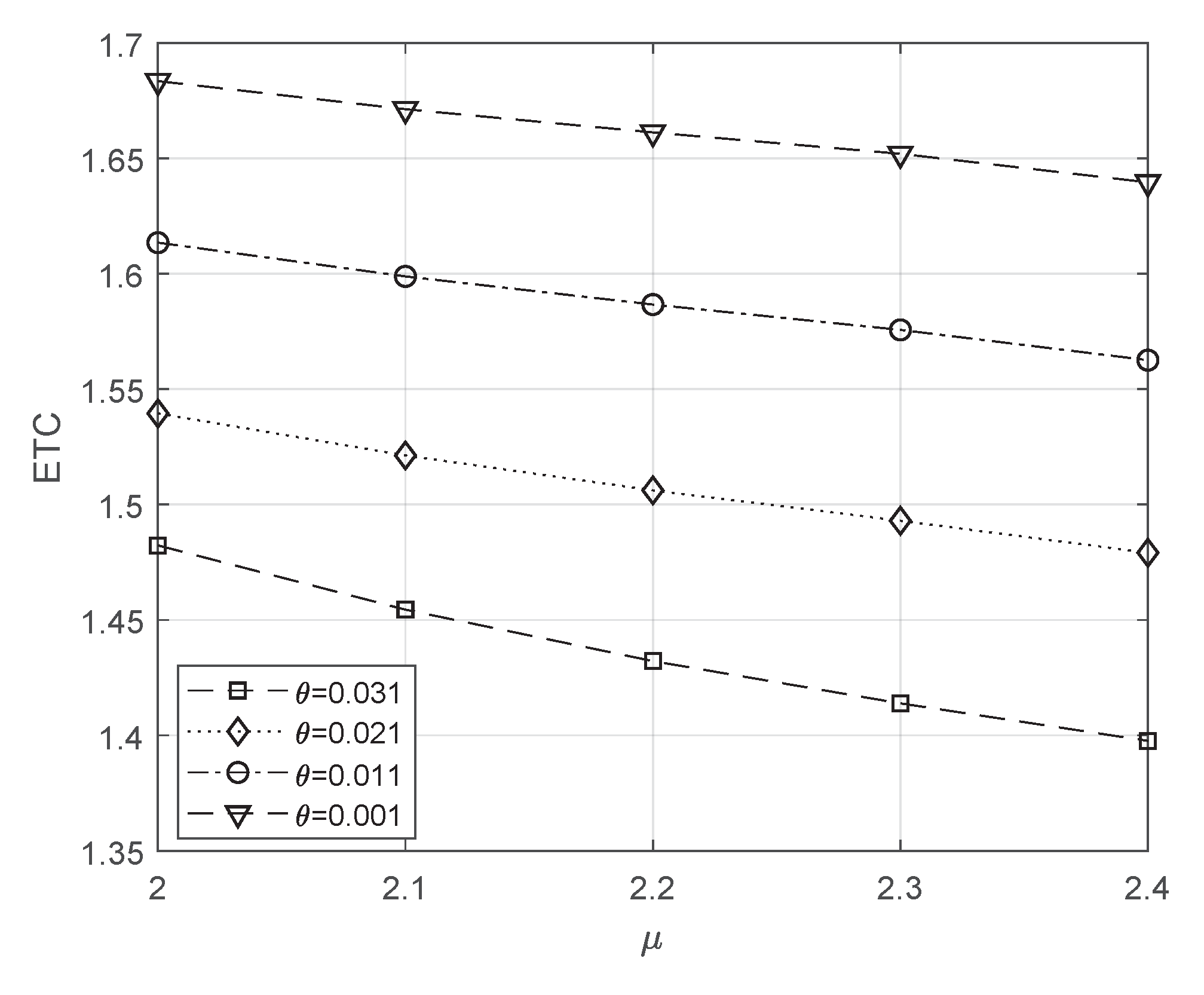
• The intensity rate, μ, causes the reduction of ETC if it increases. This is because the average service time per customer reduces if μ increases. Since it reduces the number of customer in the waiting hall and orbit, the sum of $C_{w1}*{\Lambda }_3$ and $C_{w2}*{\Lambda }_4$ are decreased. Therefore, the total cost is reduced when μ increases. This is shown in Figure 3.
• In Figure 4, θ and μ are increased simultaneously to explore the ETC. Here, the parameter θ causes the decrease in total cost when it is increased, and the parameter μ holds the same characteristic as we said in Figure 3. In Figure 4, both θ and μ hold the monotonic property.
• Furthermore, the ETC can also be determined when the probability p and queue size N are varied together in Figure 5. There is an interesting fact to notice that, when we increase the queue capacity to N, it will produce the convex values for each p. So, this helps us find the optimal N for each p.
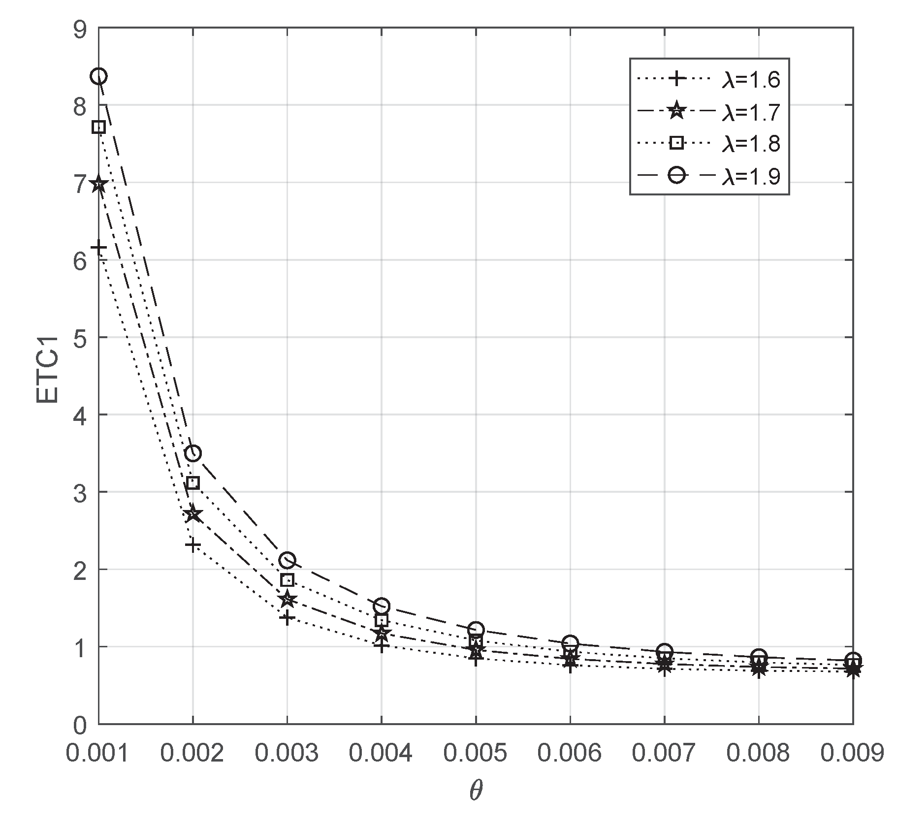
• As we discussed in the Figure 2, Figure 3, Figure 4 and Figure 5, the same parameters are discussed for the WSAM in the Figure 6, Figure 7, Figure 8 and Figure 9, respectively. The later figures express the average total cost of the WSAM, which is determined as ETC1. The characteristics of the parameters in the Figure 6, Figure 7, Figure 8 and Figure 9 hold the same property as we see in Figure 2, Figure 3, Figure 4 and Figure 5. Now, the comparison result tells us the ETC1 of the WSAM is higher than the SAM. That is the proposed model will have the minimized total cost. So, the SAM is more effective than WSAM.

From an economic point of view, the cost analysis of a business is the fundamental one. To determine such a total cost in the inventory sales business, one require various parameters and cost values as we used in this proposed model. When the researcher or business personalities study this paper, they could easily sense that what are the parameters are crucial to determine the total cost of their business. According to this analysis, they can come up with new strategies and ideas to develop their business as well.

Example 2.

This example investigates the waiting time of a customer in the waiting hall as well as the orbit when the parameters are changed.

• Table 1. Effect of $\lambda$ vs $\mu$ on the waiting time of a customer in the queue $\left({\Lambda }_3\right)$.

  $\mathit{\lambda }\setminus \mathit{\mu }$	2	2.1	2.2	2.3	2.4
  1.5	1.576759	1.535679	1.504759	1.481146	1.470391
  1.6	1.556556	1.499638	1.457448	1.425828	1.401054
  1.7	1.567412	1.489958	1.432579	1.389537	1.356815
  1.8	1.610741	1.508230	1.431498	1.373853	1.330122
  1.9	1.684501	1.555196	1.455632	1.379811	1.322041

  shows the impact of waiting time on a customer in the queue when λ and μ are increased simultaneously. The service rate reduces the customer’s waiting time whenever it increases. It should be noted that the parameter λ has both decreasing and increasing property on the waiting time of a customer if it increases. That is, λ does not hold the monotonic property for determining the waiting time of a customer in the queue. Thus, this analysis gives an optimum λ to determine the waiting time of a customer in the queue.
• If the retrial rate θ increases, then the number of customers in the queue increases, and on following this, their waiting time also increases, which is shown in

  Table 2. Effect of $\theta$ vs $\mu$ on the waiting time of a customer in the queue $\left({\Lambda }_3\right)$.

  $\mathit{\theta }\setminus \mathit{\mu }$	2	2.1	2.2	2.3	2.4
  0.0005	1.903839	1.739922	1.609444	1.508832	1.432132
  0.0055	1.862165	1.853358	1.846244	1.839181	1.827003
  0.0105	2.100453	2.095665	2.092463	2.088874	2.078800
  0.0155	2.224800	2.223188	2.222936	2.222096	2.214772
  0.0205	2.294393	2.295024	2.296835	2.298008	2.293127

  . On the other hand, when we reduce the average service time per customer, the number of customers in the waiting hall will be reduced. This will help us minimise the expected waiting time of a customer when μ increases. Here, θ and μ hold the monotonic property on the waiting time of a customer in the queue.
• When the arrival rate increases, the waiting time of customers in the orbit increases. This is because the number of customers in the queue becomes full if λ increases. It also causes a rise in the number of customers in orbit and an unsuccessful retrial process for orbit customers. Thus, their waiting time increases. Since the service rate reduces the number of customers in the queue, orbit customers can easily get into the queue. This implies that the waiting time of an orbit customer reduces whenever μ increases. These facts are shown in

  Table 3. Effect of $\lambda$ vs. $\mu$ on the waiting time of a customer in the orbit $\left({\Lambda }_4\right)$.

  $\mathit{\lambda }\setminus \mathit{\mu }$	2	2.1	2.2	2.3	2.4
  1.5	106.093100	79.775100	60.973900	46.375900	19.310100
  1.6	157.170600	122.402700	95.218400	72.397300	58.071400
  1.7	221.614900	175.658700	139.169600	110.370600	87.146700
  1.8	297.528200	241.191800	194.308100	155.994100	125.302300
  1.9	381.135100	316.564200	260.426000	212.835700	173.366700

  .
• Table 4. Effect of $\theta$ vs. $\mu$ on the waiting time of a customer in the orbit $\left({\Lambda }_4\right)$.

  $\mathit{\theta }\setminus \mathit{\mu }$	2	2.1	2.2	2.3	2.4
  0.0005	955.406536	808.208915	674.786136	557.785332	457.996943
  0.0055	12.417924	9.598283	7.436280	5.788929	4.568360
  0.0105	3.592078	2.757883	2.124736	1.646882	1.296916
  0.0155	1.710162	1.308988	1.005653	0.777490	0.611793
  0.0205	1.009319	0.770953	0.591139	0.456342	0.358528

  shows that the waiting time of a customer in the orbit when θ and μ are varied simultaneously. Here too, μ preserves its monotonic property, as we shown in Table 3. Next, when we observe θ, it reduces the customer waiting time in orbit when it increases. Because the number of orbit customers going to the queue will be successful, so, the time of a customer has to stay in orbit will be reduced.
• As the probability p increases, customers waiting time in the queue increases. If p increases, it means that the number of customers in the orbit will increase, and following this, at some random time, the number of customers entering the queue from an orbit will increase. Therefore, the probability p causes the increase of waiting time of a customer in the queue as well as the orbit whenever it increases and are shown in

  Table 5. Effect of p vs. N on the waiting time of queue.

  $\mathit{p}\setminus \mathit{N}$	8	9	10	11	12
  0.2	1.462061	1.372522	1.422151	1.585071	1.703729
  0.3	1.587034	1.431498	1.447220	1.558669	1.734880
  0.4	1.695282	1.486165	1.472691	1.570530	1.740293
  0.5	1.787840	1.536860	1.496655	1.581781	1.745522
  0.6	1.866281	1.583904	1.519254	1.592439	1.750500

  and

  Table 6. Effect of p vs. N on the waiting time of a customer in the orbit.

  $\mathit{p}\setminus \mathit{N}$	8	9	10	11	12
  0.2	388.595160	187.952874	75.836585	11.550505	10.498995
  0.3	393.056438	194.308066	89.980107	40.652257	18.233375
  0.4	399.349249	200.579255	93.780456	42.660691	19.230352
  0.5	407.115011	206.927869	97.474353	44.506608	20.100766
  0.6	416.051993	213.350897	101.138148	46.327513	20.954823

  , respectively.
• When we expand the queue size, N, we obtain the optimal N on the waiting time of a customer in the queue where as it reduces the waiting time of a customer in the orbit if we increase N. As the queue size increases, there will be an opportunity for an orbit customer to join the queue. That’s why their waiting time will be decreased. This information is obtained from Table 5 and Table 6.

In customer-oriented business services, waiting time analysis is an inevitable discussion. Without analysing this, the cost analysis cannot be effective. So, to run a successful business, the company must satisfy the customer through their service process. In this connection, the less waiting time of a customer in the company, will make them as a loyal customer. They will not move to another company. Thus, this illustration will be helpful to study the waiting time of a customer in their business.

Example 3.

This example investigates the mean inventory level and the mean reorder rate under parameter variation.

• When both parameters, λ and θ, increase, the mean inventory level reduces. Since every arrival requires an item from the inventory, the mean inventory level reduces according to the increase in arrival flow. This is shown in Figure 10.
• If the service rate μ increases, the mean inventory level reduces. Because at the time of every service completion, there will be one unit in the inventory depleted. So that mean inventory level is reduced as shown in Figure 11.
• Figure 12 shows the impact of mean inventory level when θ and μ are increased together. θ and μ hold the same characteristic as we said in Figure 10 and Figure 11, respectively.
• In Figure 13, we determine the mean inventory level under the combination of c and N. The expansion of queue capacity N reduces the mean inventory level because more number of customers can arrive to the system without lost. So, due to the increase in arrivals, the mean inventory level reduces. When we increase the number of active servers according to the queue length, the mean inventory level is reduced.

The calculation of the mean inventory level will help us place an order for replenishment at the correct time. During the time of a stock out situation, the customer in the system will have a long waiting time. Due to this stock out problem, the customer loses their patience and leaves the system without purchasing it. So, a company will always have a sharp eye to maintain the positive inventory in the system. In such a way, this means inventory level discussion will be sufficient for all inventory-selling business personalities.

• Figure 14 shows the interpretation of the parameters λ and θ. If we increase both λ and θ simultaneously, the mean reorder rate will increase. Because both λ and θ will cause a decrease in mean inventory in the system. Therefore, the replenishment process will be triggered whenever the current number of inventory falls to s.
• The service parameter μ also impacts the mean reorder rate with the same result as λ and θ as we said in Figure 14. This discussion is shown in Figure 15.
• If we increase the number of servers and queue capacity simultaneously, the mean reorder rate will increase. Because both will cause the mean inventory level to decrease. This interpretation is shown in Figure 16.
• Figure 17 explores the impact of probability p. If we increase p, the mean reorder rate will increase because it will cause the number of tagged customers to increase.

The determination of the average reorder rate will give sufficient details to the businessmen to proceed with the replenishment process in their inventory selling business. The discussion of the mean reorder rate allows us to define the set up cost and the total cost of the system. According to the results that we obtained here, every businessman will come up with a new strategy for the replenishment process in their business.

Example 4.

This example explains the expected customer lost under the parameter variation from

Table 7. Effect of system parameters on the mean number of customers lost $\left({\Lambda }_5\right)$.

c	$\mathit{\lambda }$	$\mathit{\mu }$	N	8			9			10
			p	0.3	0.4	0.5	0.3	0.4	0.5	0.3	0.4	0.5
2	1.7	2.1	0.009700		0.007798	0.006118	0.008358	0.006712	0.005261	0.007750	0.006219	0.004873
		2.2	0.008723		0.007031	0.005530	0.007681	0.006186	0.004862	0.007219	0.005817	0.004570
		2.3	0.007949		0.006423	0.005062	0.007142	0.005766	0.004542	0.006816	0.005489	0.004323
	1.8	2.1	0.011407		0.009137	0.007146	0.009493	0.007593	0.005931	0.008583	0.006860	0.005356
		2.2	0.010118		0.008128	0.006373	0.008610	0.006909	0.005412	0.007920	0.006352	0.004973
		2.3	0.009099		0.007329	0.005760	0.007912	0.006367	0.005000	0.007384	0.005943	0.004665
	1.9	2.1	0.013549		0.010814	0.008430	0.010914	0.008695	0.006768	0.009607	0.007646	0.005947
		2.2	0.011867		0.009501	0.007427	0.009764	0.007806	0.006094	0.008759	0.006997	0.005459
		2.3	0.010539		0.008461	0.006631	0.008862	0.007106	0.005563	0.008088	0.006482	0.005072
3	1.7	2.1	0.008009		0.006454	0.005074	0.007329	0.005899	0.004635	0.007071	0.005671	0.004454
		2.2	0.007457		0.006021	0.004742	0.006930	0.005598	0.004407	0.006634	0.005424	0.004271
		2.3	0.007006		0.005667	0.004470	0.006625	0.005343	0.004213	0.006562	0.005215	0.004110
	1.8	2.1	0.008938		0.007186	0.005639	0.007928	0.006366	0.004989	0.007500	0.006022	0.004719
		2.2	0.008231		0.006630	0.005211	0.007459	0.006002	0.004713	0.007144	0.005743	0.004509
		2.3	0.007662		0.006183	0.004868	0.007060	0.005698	0.004483	0.006775	0.005500	0.004327
	1.9	2.1	0.010089		0.008094	0.006340	0.008640	0.006919	0.005411	0.008018	0.006418	0.005017
		2.2	0.009180		0.007378	0.005789	0.008061	0.006470	0.005069	0.007594	0.006090	0.004770
		2.3	0.008455		0.006808	0.005350	0.007588	0.006103	0.004791	0.007240	0.005812	0.004561
4	1.7	2.1	0.007823		0.006302	0.004953	0.007251	0.005835	0.004584	0.007050	0.005639	0.004429
		2.2	0.007329		0.005916	0.004659	0.006874	0.005555	0.004373	0.006621	0.005402	0.004254
		2.3	0.006918		0.005594	0.004413	0.006582	0.005313	0.004190	0.006487	0.005199	0.004098
	1.8	2.1	0.008629		0.006935	0.005440	0.007790	0.006255	0.004903	0.007427	0.005966	0.004675
		2.2	0.008015		0.006454	0.005071	0.007366	0.005927	0.004654	0.007095	0.005705	0.004480
		2.3	0.007510		0.006059	0.004769	0.006994	0.005647	0.004443	0.006735	0.005474	0.004308
	1.9	2.1	0.009604		0.007701	0.006030	0.008414	0.006738	0.005269	0.007901	0.006325	0.004944
		2.2	0.008833		0.007096	0.005565	0.007907	0.006346	0.004972	0.007520	0.006027	0.004721
		2.3	0.008207		0.006606	0.005189	0.007482	0.006017	0.004723	0.007200	0.005770	0.004528

.

• The arrival rate, λ, induces the increase of customers lost whenever it increases. Due to the finite capacity of queue size, the mean customers lost will increase if the number of customers in the queue increases.
• The mean customer loss is reduced when the service rate μ increases. Since the average service time per customer reduces, the number of customers in the queue will be reduced, and this will reduce the mean customers lost.
• If we increase the number of servers in the system, an arriving customer need not wait a long time in the queue. This process will always keep available space in the queue. Thus, the mean number of customers lost will be controlled.
• The probability value, p, increases, meaning that, whenever the queue size is full, an arriving new customer chooses the orbit is increased. Thus, the mean customer loss is reduced.
• Suppose we expand the queue size N, there will be more number of customers utilize the queue to purchase the item. So that, the mean customer lost is decreased when N is increased.

Generally, in every business, customers are the pillars. If the number of customers approaching the business increases, the profit will also increase. Hence, to promote a successful business, one has to think about reducing the number of customers lost. In such a way, this example will be helpful in gaining knowledge about customers lost in the business.

Example 5.

The fraction of successful rate of retrial and the mean number of busy servers are discussed in this example using the

Table 8. Influence of $\lambda ,\mu$ and $\theta$ on the fraction of successful rate of retrials and mean number of active servers for $c=2$.

$\mathit{\mu }$	${\mathit{\Lambda }}_8$	${\mathit{\Lambda }}_9$	$\mathit{\theta }$	${\mathit{\Lambda }}_8$	${\mathit{\Lambda }}_9$	$\mathit{\lambda }$	${\mathit{\Lambda }}_8$	${\mathit{\Lambda }}_9$
2.0	0.924652	1.509372	0.0005	0.926486	1.505065	1.2	0.927840	1.467337
2.1	0.925057	1.505671	0.2005	0.906107	0.736203	1.3	0.925825	1.468823
2.2	0.925359	1.501759	0.4005	0.889334	0.602129	1.4	0.925491	1.475423
2.3	0.925584	1.497738	0.6005	0.874788	0.595621	1.5	0.925493	1.482729
2.4	0.925748	1.493682	0.8005	0.861598	0.609241	1.6	0.925551	1.489820
2.5	0.925862	1.489640	1.0005	0.849302	0.624767	1.7	0.925504	1.496158
2.6	0.925954	1.485699	1.2005	0.837679	0.638703	1.8	0.925359	1.501759
2.7	0.926009	1.481820	1.4005	0.826657	0.650591	1.9	0.925118	1.506626
2.8	0.925941	1.477725	1.6005	0.816216	0.660628	2.0	0.924780	1.510765
2.9	0.926267	1.475065	1.8005	0.806355	0.669130	2.1	0.924328	1.514183

,

Table 9. Influence of $\lambda ,\mu$ and $\theta$ on the fraction of successful rate of retrials and mean number of active servers for $c=3$.

$\mathit{\mu }$	${\mathit{\Lambda }}_8$	${\mathit{\Lambda }}_9$	$\mathit{\theta }$	${\mathit{\Lambda }}_8$	${\mathit{\Lambda }}_9$	$\mathit{\lambda }$	${\mathit{\Lambda }}_8$	${\mathit{\Lambda }}_9$
2.0	0.926075	1.657379	0.0005	0.763936	0.820296	1.2	0.928479	1.650535
2.1	0.926228	1.653234	0.2005	0.740178	0.677656	1.3	0.927088	1.644416
2.2	0.926345	1.649974	0.4005	0.736420	0.690094	1.4	0.926598	1.641717
2.3	0.926435	1.647448	0.6005	0.722663	0.715789	1.5	0.925008	1.641391
2.4	0.926509	1.645536	0.8005	0.708905	0.738132	1.6	0.924517	1.643749
2.5	0.926543	1.644052	1.0005	0.690147	0.755946	1.7	0.923027	1.646555
2.6	0.926674	1.643285	1.2005	0.681389	0.770079	1.8	0.921937	1.649974
2.7	0.926653	1.642424	1.4005	0.667632	0.781438	1.9	0.920846	1.654020
2.8	0.926336	1.640781	1.6005	0.660874	0.790716	2.0	0.919756	1.658656
2.9	0.927392	1.640379	1.8005	0.640116	0.798412	2.1	0.918666	1.663835

and

Table 10. Influence of $\lambda ,\mu$ and $\theta$ on the fraction of successful rate of retrials and mean number of active servers for $c=4$.

$\mathit{\mu }$	${\mathit{\Lambda }}_8$	${\mathit{\Lambda }}_9$	$\mathit{\theta }$	${\mathit{\Lambda }}_8$	${\mathit{\Lambda }}_9$	$\mathit{\lambda }$	${\mathit{\Lambda }}_8$	${\mathit{\Lambda }}_9$
2	0.926602	2.009274	0.0005	0.927680	1.997852	1.2	0.928501	1.984804
2.1	0.926737	2.002294	0.2005	0.913159	1.925373	1.3	0.927538	1.987657
2.2	0.926839	2.004455	0.4005	0.902023	1.875666	1.4	0.927149	1.990490
2.3	0.926917	2.001869	0.6005	0.892417	1.828771	1.5	0.926703	1.993255
2.4	0.926979	1.999858	0.8005	0.883388	1.776558	1.6	0.926812	1.995904
2.5	0.927002	1.997999	1.0005	0.874622	1.718074	1.7	0.926844	1.998322
2.6	0.927117	1.995748	1.2005	0.866097	1.655190	1.8	0.926839	2.000144
2.7	0.927098	1.993258	1.4005	0.857916	1.590568	1.9	0.926807	2.005162
2.8	0.927728	1.990483	1.6005	0.850174	1.526421	2.0	0.926743	2.009853
2.9	0.928656	1.987423	1.8005	0.842948	1.464404	2.1	0.926645	2.017364

.

• The service parameter μ will cause an increase of ${\Lambda }_8$ for retrial customers. Since the average service time per customer is reduced, the number of available places in the queue will increase. So, the retrial customer approaching the system will also be successful. On the other hand, the mean number of busy servers is decreased when μ is increased. It helps to reduce the number of customers in the queue. As the size of the queue decreases, the active server will be deactivated soon. That is why the mean number of busy servers will be reduced if μ is increased.
• The retrial rate θ induce the decrease of ${\Lambda }_8$ if it increases. This decrement happened due to the impact of the successful rate of retrial and the overall rate of retrial. Both will increase if θ increases. In this situation, the rate of increase in the overall rate of retrial is faster than the rate of successful rate of retrial. Due to this difference, the fraction of successful rate of retrial will decrease when θ increases.
• When λ increases, the ${\Lambda }_8$ will be decreased. Because the occurrence of primary arrival causes the non-availability of the space in the queue. This implies that the successful rate of retrial will be decreased. Therefore, ${\Lambda }_8$ is reduced if λ increases. The mean number of active servers will be increased as the queue size increases. This is because the increase in arrivals reaches the next threshold level as soon as it does. So, the new server will be activated according to the queue length.
• Furthermore, if we increase the number of active servers according to the queue length, the fraction of the successful rate of retrial and the mean number of busy servers will increase. This is because, according to the increased number of busy servers, the number of customers in the queue will be reduced. This will give the retrial customer an opportunity to enter the waiting hall. Thus, their fraction of successful rate of retrial will increase. Similarly, the mean number of active servers also increases.

The study of the fraction of the successful rate of retrial and the mean number of busy servers in a retrial system will give efficient information to business people. According to the effects of the parameter on ${\Lambda }_8$ and ${\Lambda }_9$, we will frame new strategies and ideas for their business. Since the retrial queue is a virtual queue, one cannot predict its nature and its influences on the system. Therefore, this fraction of successful rate of retrial analysis will be helpful to the businessmen observing the retrial queue.

7. Conclusions

A detailed analysis of the server activation/deactivation in the MQIS has been discussed in this paper based on the multi-threshold levels. Using the matrix geometric approach, the steady-state probability vectors are derived to compute the characteristics of this model. The $n^{th}$ moment of the waiting hall and orbit are derived by applying LST. Generally, the maintenance and adoption of a multi-server service facility is not an easy task for many businesses. In such businesses, the owners are mostly willing to appoint the temporary servers as for their necessity only. This idea can be easily seen from our real-life scenarios like contract based workers, labourers, the increase of more bus and train services during the peak hours, increasing ticket counters in the railway station, and so on. The mentioned service facilities are not always available for a long time. According to this fact, the proposed model was developed to study the activation and deactivation of servers. In addition, we provided the generalised results for both SAM and WSAM.

7.1. Limitations and Prospects of the Model

The study of a recruiting temporary server in a company will have the following limitations and prospects.

• The activation/deactivation of the server is triggered whenever the corresponding queue length hits the respective threshold level. Mostly, the system manager uses the server if there is a requirement. Otherwise, the servers are not used. This strategy will reduce the cost of the servers in the business, and the average total cost of the business is also controlled.
• Since some servers’ working durations are very short, the company has the chance to earn more profit. Because the servers will be deactivated as soon as the queue length is reduced.
• During the deactivation period of the server, the system manager may utilize the server to do the other pending tasks in the system. This idea also helps us to increase the system’s profit rate.
• Even though we provide a generalized result for SAM and WSAM, this model is completely different from the regular multi-server model or WSAM. This is because the key idea of this study is to analyse the impact of the temporary servers on the business service. In real-life, many business services are available related to our proposed model (see online food delivery business, online shopping business, and so on). As for their needs, they increased their servers. So the comparative study between SAM and WSAM will not be an effective one.
• The cost analysis between SAM and WSAM under the parameter variation shows that SAM helps us to minimize the total cost of the system. That is why many business people recruit part-time workers in their business services.
• There will be an opportunity to study the variance of the waiting time of a customer by using the $n^{th}$ moment of waiting time distribution. This variance discussion will give a clear idea about their waiting time.

7.2. Remarks on the Results

Through both are different models, from the comparison, we see that the SAM is more efficient than the WSAM. The numerical study on the total cost shows us that the assumed SAP minimises the total cost of the business. The course of necessary characteristics such as waiting time for customers in the orbit and waiting hall, mean customer loss, mean reorder rate, and fraction of successful retrial rate suggests a businessman adapting a new technique for increasing the growth rate and customer satisfaction. Over these outcomes, SAP controls the workload of the server, which ensures the enthusiastic performance of the server. So, the customer will receive satisfied service when the server works happily, which will build a good customer relationship with the business. As the utilisation of the servers in the inventory-based business is reduced, it guarantees more profit to the business. It will definitely increase the number of loyal customers to the system, which assures that the company will earn a good profit.

7.3. Future Direction

During the time of the deactivation of the server, the system manager may provide a vacation for the server. Suppose that when the queue length hits the next threshold level when the server is on vacation, the system manager abruptly interrupts his vacation.

References

1. Melikov, A.Z.; Molchanov, A.A. Stock optimization in transport/storage. Cybern. Syst. Anal. 1992, 28, 484–487. [Google Scholar] [CrossRef]
2. Sigman, K.; Simchi-Levi, D. Light traffic heuristic for an M/G/1 queue with limited inventory. Ann. Oper. Res. 1992, 40, 371–380. [Google Scholar] [CrossRef]
3. Lawrence, A.S.; Sivakumar, B.; Arivarignan, G. A perishable inventory system with service facility and finite source. Appl. Math. Model. 2013, 37, 4771–4786. [Google Scholar] [CrossRef]
4. Krishnamoorthy, A.; Joshua, A.N.; Kozyrev, D. Analysis of a Batch Arrival, Batch Service Queuing-Inventory System with Processing of Inventory While on Vacation. Mathematics 2021, 9, 219. [Google Scholar] [CrossRef]
5. Jeganathan, K.; Selvakumar, S.; Anbazhagan, N.; Amutha, S.; Hammachukiattikul, P. Stochastic modeling on M/M/1/N inventory system with queue-dependent service rate and retrial facility. AIMS Math. 2021, 6, 7386–7420. [Google Scholar] [CrossRef]
6. Sugapriya, C.; Nithya, M.; Jeganathan, K.; Anbazhagan, N.; Joshi, G.P.; Yang, E.; Seo, S. Analysis of Stock-Dependent Arrival Process in a Retrial Stochastic Inventory System with Server Vacation. Processes 2022, 10, 176. [Google Scholar] [CrossRef]
7. Amirthakodi, M.; Sivakumar, B. An inventory system with service facility and feedback customers. Int. J. Ind. Syst. Eng. 2019, 33, 374–411. [Google Scholar] [CrossRef]
8. Chakravarthy, S.R.; Maity, A.; Gupta, U.C. An ‘(s, S)’ inventory in a queueing system with batch service facility. Ann. Oper. Res. 2017, 258, 263–283. [Google Scholar] [CrossRef]
9. Jeganathan, K.; Reiyas, M.A.; Padmasekaran, S.; Lakshmanan, K. An M/EK/1/N Queueing-Inventory System with Two Service Rates Based on Queue Lengths. Int. J. Appl. Comput. Math. 2017, 3, 357–386. [Google Scholar] [CrossRef]
10. Jeganathan, K.; Reiyas, M.A.; Selvakumar, S.; Anbazhagan, N. Analysis of Retrial Queueing-Inventory System with Stock Dependent Demand Rate: (s, S) Versus (s, Q) Ordering Policies. Int. J. Appl. Comput. Math. 2020, 6, 1–29. [Google Scholar] [CrossRef]
11. Krishnamoorthy, A.; Manikandan, R.; Lakshmy, B. A revisit to queueing-inventory system with positive service time. Ann. Oper. Res. 2015, 233, 221–236. [Google Scholar] [CrossRef]
12. Sangeetha, N.; Sivakumar, B. Optimal service rates of a perishable inventory system with service facility. Int. J. Math. Oper. Res. 2020, 16, 515–550. [Google Scholar] [CrossRef]
13. Yadavalli, V.S.S.; Jeganathan, K.; Venkatesan, T.; Padmasekaran, S.; Jehoashan Kingsly, S. A retrial queueing-inventory system with J-additional options for service and finite source. ORiON 2017, 33, 105–135. [Google Scholar] [CrossRef]
14. Liu, Z.; Luo, X.; Wu, J. Analysis of an M/PH/1 Retrial Queueing-Inventory System with Level Dependent Retrial Rate. Math. Probl. Eng. 2020, 2020, 1–10. [Google Scholar] [CrossRef]
15. Jeganathan, K.; Abdul Reiyas, M.; Prasanna Lakshmi, K.; Saravanan, S. Two server Markovian inventory systems with server interruptions:Heterogeneous vs. homogeneous servers. Math. Comput. Simul. 2019, 155, 177–200. [Google Scholar] [CrossRef]
16. Jeganathan, K.; Melikov, A.Z.; Padmasekaran, S.; Jehoashan Kingsly, S.; Prasanna Lakshmi, K. A Stochastic Inventory Model with Two Queues and a Flexible Server. Int. J. Appl. Comput. Math. 2019, 5, 1–27. [Google Scholar] [CrossRef]
17. Jeganathan, K.; Reiyas, M.A. Two parallel heterogeneous servers Markovian inventory system with modified and delayed working vacations. Math. Comput. Simul. 2020, 172, 273–304. [Google Scholar] [CrossRef]
18. Jeganathan, K.; Selvakumar, S.; Saravanan, S.; Anbazhagan, N.; Amutha, S.; Cho, W.; Joshi, G.P.; Ryoo, J. Performance of Stochastic Inventory System with a Fresh Item, Returned Item, Refurbished Item, and Multi-Class Customers. Mathematics 2022, 10, 1137. [Google Scholar] [CrossRef]
19. Krishnamoorthy, A.; Manikandan, R.; Shajin, D. Analysis of a Multi-server Queueing-Inventory System. Adv. Oper. Res. 2015, 2015, 1–16. [Google Scholar] [CrossRef]
20. Yadavalli, V.S.S.; Sivakumar, B.; Arivarignan, G.; Adetunji, O. A finite source multi-server inventory system with service facility. Comput. Ind. Eng. 2012, 63, 739–753. [Google Scholar] [CrossRef]
21. Wang, F.; Bhagat, A.; Chang, T. Analysis of priority multi-server retrial queueing inventory systems with MAP arrivals and exponential services 2012, OPSEARCH. In Operational Research Society of India; Springer: Berlin/Heidelberg, Germany, 2017; Volume 54, pp. 44–66. [Google Scholar]
22. Nair, A.N.; Jaccob, M.J. On the distribution of an (r,Q) inventory with lead time via multi server queues. Int. J. Intell. Enterp. 2015, 3, 3–18. [Google Scholar] [CrossRef]
23. Chakravarthy, S.R.; Shajin, D.; Krishnamoorthy, A. Infinite Server Queueing-Inventory Models. J. Indian Soc. Probab. Stat. 2020, 21, 43–68. [Google Scholar] [CrossRef]
24. Wang, F. Approximation and Optimization of a Multi-Server Impatient Retrial Inventory-Queueing System with Two Demand Classes. Qual. Technol. Quant. Manag. 2015, 12, 269–292. [Google Scholar] [CrossRef]
25. Hanukov, G.; Avinadav, T.; Chernonog, T.; Yechiali, U. A multi-server queueing-inventory system with stock-dependent demand. IFAC-PapersOnLine 2019, 52, 671–676. [Google Scholar] [CrossRef]
26. Nair, A.N.; Jacob, M.J.; Krishnamoorthy, A. The multi server M/M/(s,S) queueing inventory system. Ann. Oper. Res. 2013, 233, 321–333. [Google Scholar] [CrossRef]
27. Paul, M.; Sivakumar, B.; Arivarignan, G. A Multi-Server Perishable Inventory SystemWith Service Facility. Pac. J. Appl. Math. 2009, 2, 69–82. [Google Scholar]
28. Rajkumar, M.; Sivakumar, B.; Arivarignan, G. An infinite queue at a multi-server inventory system. Int. J. Inventory Res. 2014, 2, 189–221. [Google Scholar] [CrossRef]
29. Rasmi, K.; Jacob, M.J. Analysis of a multiserver queueing inventory model with self-service. Int. J. Math. Model. Numer. Optim. 2021, 11, 275–291. [Google Scholar] [CrossRef]
30. Jeganathan, K.; Harikrishnan, T.; Selvakumar, S.; Anbazhagan, N.; Amutha, S.; Acharya, S.; Dhakal, R.; Joshi, G.P. Analysis of Interconnected Arrivals on Queueing-Inventory System with Two Multi-Server Service Channels and One Retrial Facility. Electronics 2021, 10, 576. [Google Scholar] [CrossRef]
31. Wang, K.H.; Tai, K.Y. A queueing system with queue-dependent servers and finite capacity. Appl. Math. Model. 2000, 24, 807–814. [Google Scholar] [CrossRef]
32. Jain, M. Finite Capacity M/M/r Queueing System with Queue-Dependent Servers. Comput. Math. Appl. 2005, 50, 187–199. [Google Scholar] [CrossRef] [Green Version]
33. Wei, F. Algorithm for waiting time distribution of a discrete-time multi-server queue with deterministic service times and multi-threshold service policy. Procedia Comput. Sci. 2011, 4, 1383–1392. [Google Scholar] [CrossRef] [Green Version]
34. Chakravarthy, S.R. A Multi-Server Queueing Model With Markovian Arrivals and Multiple Thresholds. Asia-Pac. J. Oper. Res. 2007, 24, 223–243. [Google Scholar] [CrossRef]
35. Neuts, M.F. Matrix-Geometric Solutions in Stochastic Models—An Algorithmic Approach; Dover Publication Inc.: New York, NY, USA, 1981. [Google Scholar]
36. Lopez-Herrero, M.J. Waiting time and other first-passage time measures in an (s,S) inventory system with repeated attempts and finite retrial group. Comput. Oper. Res. 2010, 37, 1256–1261. [Google Scholar] [CrossRef]
37. Abate, J.; Whitt, W. Numerical inversion of Laplace transformation of probability distributions. ORSA J. Comput. 1995, 7, 36–43. [Google Scholar] [CrossRef] [Green Version]
Figure 1. Graphical depiction of the model.
Mathematics 10 02682 g001
Figure 2. The impact of ETC when λ vs θ for SAM.
Mathematics 10 02682 g002
Figure 3. The impact of ETC when λ vs μ for SAM.
Mathematics 10 02682 g003
Figure 4. The impact of ETC when θ vs μ . for SAM.
Mathematics 10 02682 g004
Figure 5. The impact of ETC when N vs p for SAM.
Mathematics 10 02682 g005
Figure 6. The impact of ETC when λ vs θ for WSAM.
Mathematics 10 02682 g006
Figure 7. The impact of ETC when λ vs μ for WSAM.
Mathematics 10 02682 g007
Figure 8. The impact of ETC when θ vs μ for WSAM.
Mathematics 10 02682 g008
Figure 9. The impact of ETC when N vs p for WSAM.
Mathematics 10 02682 g009
Figure 10. The impact of mean inventory level when λ vs. θ .
Mathematics 10 02682 g010
Figure 11. The impact of mean inventory level when λ vs. μ .
Mathematics 10 02682 g011
Figure 12. The impact of mean inventory level when θ vs. μ .
Mathematics 10 02682 g012
Figure 13. The impact of mean inventory level when N vs. c.
Mathematics 10 02682 g013
Figure 14. The impact of mean reorder rate when λ vs. θ .
Mathematics 10 02682 g014
Figure 15. The impact of mean reorder rate when λ vs. μ .
Mathematics 10 02682 g015
Figure 16. The impact of mean reorder rate when N vs. c.
Mathematics 10 02682 g016
Figure 17. The impact of mean reorder rate when N vs. p.
Mathematics 10 02682 g017