Different Modes of Combustion Wave on a Lattice Burner

Abstract

The stabilization of a planar premixed flame front on a lattice (porous) burner is considered. The developed model captures all the important features of the phenomenon, while also admitting qualitative analytical investigation. It has been rigorously mathematically proven that there exist two different stabilization regimes: one with flame front located nearby the surface of the burner, and another with the flame front located inside the lattice. These two regimes result in qualitatively different gas temperature profiles along the flow that is monotonic and non-monotonic, respectively. The boundary between the two regimes is described in terms of dependence of the lattice solid material temperature on flow Peclet number. With similar temperature profiles, such dependencies may be both monotonic and non-monotonic. The transition between the two types of dependencies is controlled by the Arrhenius number. Conclusions of the study are supported by numerical analysis. They also compare favorably with the available experimental data. The novelty of the present approach is a fundamentally rigorous analytical analysis of the problem. The proposed analytical model, based on $\delta$-function approximation of the chemical source term, agrees well (within 7% relative error) with the model based on the distributed description of the chemical reaction zone. The obtained results are important from both a theoretical and practical point of view. They demonstrate the existence of the two qualitatively different operating regimes for lattice burners, thus impacting design solutions for such devices. The results will be of great interest to the broader academic community, particularly in research areas where similar wave structures may emerge.

1. Introduction

Combustion waves are a natural way of flame spread. The most basic of such structures is the laminar pre-mixed flame propagating through a pipe or channel [1,2,3,4]. The most common dominant mechanism of such propagation is heat conduction from the flame front to the adjacent pre-heat zone, raising the temperature of the latter to values supporting a significant increase in the mixture reaction rate. This type of wave structure is known as a thermal flame. An alternative driving mechanism is the diffusion propagation of active radicals away from the reaction zone, which may support the flame being essentially driven by chain reactions, or the so-called chain flame.

A very specific standing combustion wave emerges around the burning fuel droplet [1]. More exotic examples are represented by cold or isothermal flames [3].

Flame fronts may also propagate through purely solid phase upon availability of both a solid-state reagent and oxidizer. The most important of such processes are the combustion of solid propellants [5], and the so-called Self-Propagating High-Temperature Synthesis (SPHTS) [4,6]. Combustion propagation in these cases is driven exclusively by heat conduction, with no convective effects (in the laboratory frame). Despite considerable simplification of the heat transfer mechanism, the flames of propellants, for example, are known to be capable of exhibiting very complicated dynamics, including chaotic dynamics [5].

A peculiar combustion wave is observed in fires, where propagation occurs in two-phase media, involving heat feedback from the gaseous diffusion flame to pyrolyzing solid material, which, in turn, supplies reactants back to flame [7,8].

The investigation of combustion waves with homogeneous multi-phase heat exchange within the wave structure has been somewhat more recent. One type of this process is convective combustion, where reacting gases interact with either the combustible or inert matrix of porous material [9,10,11,12,13,14].

Another is standing a combustion wave developing on a lattice (porous) burner (Figure 1). The latter device is of significant importance, both theoretically and practically.

The combustion process in porous burners has been studied extensively [15,16,17,18,19,20,21,22,23,24,25,26,27,28,29,30,31,32,33,34,35], using both experimental and numerical modelling methods, with respect to different burner configurations, combustion regimes and employed fuels (for example, biofuels).

Barra et al. [31] investigated the effects of material properties on flame stabilization in porous burners. Significant influence of thermal conductivity, the volumetric heat transfer coefficient and the radiative extinction coefficient on stable operation limits were observed.

Barra and Ellzey [32] studied the heat recirculation process, due to solid matrix, for a range of equivalence ratios. They found that recirculation efficiency decreases with the increase of the equivalence ratio.

Djordjevic et al. [35] investigated flame stability in porous burners employing various ceramic sponge-like structures. They proposed a simple criterion for prediction of blow-off limits in combustion systems employing the porous burner concept.

Of particular interest are the results of Yakovlev et al. [15], Mital et al. [17] and Janvekar et al. [27], who observed (both numerically and experimentally) non-monotonic temperature profiles within the burner. Keshtkar et al. [34] also observed non-monotonic temperature profiles in the course of their numerical analysis of rectangular two-dimensional porous radiant burners.

Existence of both monotonic and non-monotonic temperature profiles is a key focus of the present study.

Recently, Arutyunov et al. [36], using numerical methods, investigated the nature of the upper limit of methane–air mixture combustion on a flat porous lattice. They demonstrated that the position of the flame front, relative to the lattice surface, depends strongly on the heat exchange rate between the gas and the solid lattice material. Within certain ranges of fuel preheating and injection rates unstable combustion regimes were observed. Further, Shmelev [37] established, numerically, the region of stable combustion for the same system. It was shown that this region covers a wide range of gas injection velocities and expands with increase of the width of the burner.

Despite the substantial volume of research referenced above, rigorous analytical studies of such a combustion system have not been conducted.

The present paper investigates combustion wave structure on a lattice (that is, on a laminar premixed porous burner).

The novelty and contribution of the study are as follows:

• Development of tractable (admitting analytical qualitative investigation) model of combustion wave stabilizing on a lattice (porous) burner;
• Development of approximated model, based on the description of chemical source term with $\delta$-function, admitting an exact analytical solution, and the explicit construction of such a solution;
• Rigorous mathematical proof of existence of the two distinctive combustion wave modes, with monotonic and non-monotonic temperature profiles, respectively;
• Definition of critical curve in the space of control parameters, separating the two wave modes. Rigorous mathematical proof of existence of both monotonic and non-monotonic critical curves.

The existence of double-mode wave structure, rigorously proven in the present paper, agrees qualitatively with experimental evidence, as discussed below. This finding impacts design solutions for industrial porous burners.

The paper is organized in the following way. The mathematical formulation of the problem is developed in Section 2. The results and discussion are presented in Section 3 (this section is separated into formal mathematical proof (Section 3.1), numerical illustration of the results (Section 3.2), analysis of the critical curve separating the two combustion regimes (Section 3.3) and comparison with experimental data (Section 3.4)). These sections are followed by the Conclusion Section, References and Appendix A.

2. Mathematical Formulation

Assuming one-dimensional flow structure and uniform material properties (of both the gas and the solid lattice), the following steady-state Heat Transfer Equation (HTE) is considered to model the combustion process (we remind that waved variables are dimensional; see subsection Ascents in the Notation table).

$$\tilde{\lambda }\frac{d^2\tilde{T}}{d{\tilde{x}}^2}-\tilde{\rho }{\tilde{c}}_p\tilde{u}\frac{d\tilde{T}}{d\tilde{x}}+\tilde{Q}\tilde{A}{\tilde{C}}^2{\left(\tilde{T}-{\tilde{T}}_0\right)}^{1/2}\exp \left(-\frac{\tilde{E}}{\tilde{R}\tilde{T}}\right)+\tilde{h}\tilde{S}\left({\tilde{T}}_s-\tilde{T}\right)=0$$

(1)

$$\tilde{h}=\left\{\begin{array}{l}{\tilde{h}}_s>0;\hspace{0.17em}\hspace{0.17em}\tilde{x}\in \left[0,{\tilde{x}}_1\right]\\ 0;\hspace{0.17em}\hspace{0.17em}\tilde{x}\in \left({\tilde{x}}_1,\infty \right]\end{array}\right.$$

Flow is directed from left to right, and the lattice occupies the region from $0$ to ${\tilde{x}}_1$ (Figure 1).

The assumption of one-dimensional flow structure is standard in analysis of various types of combustion waves (see, for example, Zeldovich et al. [3]) and is known to lead to quantitatively correct and verifiable results. The major reason behind the assumption of uniform (e.g., temperature-independent) thermophysical properties is that is allows formal mathematical proof, presented below, to be conducted. Note, however, that this assumption is very reasonable everywhere in the flow, except for extremely narrow chemical reaction zone, as the temperature outside this zone does not deviate much from the inflow temperature.

The third term on the Left-Hand Side (LHS) of Equation (1) describes the contribution from a bimolecular reaction occurring in the premixed stream. The concentrations ${\tilde{C}}_1$ and ${\tilde{C}}_2$ of both reactants are assumed to be equal at all times, i.e., ${\tilde{C}}_1\left(\tilde{x}\right)={\tilde{C}}_2\left(\tilde{x}\right)=\tilde{C}\left(\tilde{x}\right)$. This means that combustion is being considered as stoichiometric. This assumption is made to allow for more concise mathematical proof but is not binding. The proof may be modified to remove this assumption. The fourth term describes heat transfer process between the gas and the solid lattice, with the heat transfer coefficient being assumed constant.

The chemical reaction rate is written in the form that makes it vanish at the initial temperature ${\tilde{T}}_0$. This is a standard assumption in the combustion theory.

The kinetic equation is

$$-\tilde{u}\frac{d\tilde{C}}{d\tilde{x}}=\tilde{A}{\tilde{C}}^2{\left(\tilde{T}-{\tilde{T}}_0\right)}^{1/2}\exp \left(-\frac{\tilde{E}}{\tilde{R}\tilde{T}}\right)$$

(2)

Further simplification, which is being made is that variable concentration $\tilde{C}$, is replaced on the Right-Hand Side (RHS) of Equation (2) by its initial value $\tilde{C}\equiv {\tilde{C}}_0\equiv$ const. This is reasonable in the view of much stronger dependence on reaction rate on temperature, compared to dependence on reactant concentrations.

The simplified kinetic equation takes the form

$$-\tilde{u}\frac{d\tilde{C}}{d\tilde{x}}=\tilde{A}{\tilde{C}}_0^2{\left(\tilde{T}-{\tilde{T}}_0\right)}^{1/2}\exp \left(-\frac{\tilde{E}}{\tilde{R}\tilde{T}}\right)$$

(3)

The following non-dimensional (scaling) variables are introduced

$$\xi =\frac{\tilde{x}}{{\tilde{x}}_1}\theta =\frac{\tilde{T}-{\tilde{T}}_0}{\left(\tilde{R}{\tilde{T}}_0^2/\tilde{E}\right)}Pe=\frac{{\tilde{x}}_1\tilde{u}}{\tilde{\kappa }}C=\frac{\tilde{C}}{{\tilde{C}}_0}$$

$$A=\tilde{Q}\tilde{A}{\tilde{C}}_0^2\frac{{\tilde{x}}_1^2}{\tilde{\lambda }}{\left(\frac{\tilde{R}{\tilde{T}}_0^2}{\tilde{E}}\right)}^{-1/2}\cdot \exp \left(-\frac{\tilde{E}}{\tilde{R}{\tilde{T}}_0}\right); h=\frac{\tilde{h}\tilde{S}{\tilde{x}}_1^2}{\tilde{\lambda }}$$

(4)

$$g=\frac{{\tilde{x}}_1^2}{\tilde{\kappa }}\tilde{A}{\tilde{C}}_0{\left(\frac{\tilde{R}{\tilde{T}}_0^2}{\tilde{E}}\right)}^{1/2}\cdot \exp \left(-\frac{\tilde{E}}{\tilde{R}{\tilde{T}}_0}\right)$$

The choice of the spatial scale (lattice width) and the reactant concentration scale (initial concentration) is natural. The temperature scale is chosen in the way that is commonly adopted (and reflecting most important scale) in combustion theory (see, for example, Merzhanov, and Khaikin [4]), as the ratio of excess temperature to characteristic temperature interval. Once these three scales are fixed, the other scales in Equation (4) are determined uniquely (to within an explicit inclusion of the reaction rate at initial temperature into the parameter $A$, which is also a common practice). Note that the emerging Peclet number $Pe$ is a standard parameter in the analysis of convective heat transfer problems.

The problem formulation becomes

$$\frac{d^2\theta }{d{\xi }^2}-Pe\frac{d\theta }{d\xi }+Af\left(\theta \right)C^2\left(\theta \right)H\left(C\right)+h\left({\theta }_s-\theta \right)=0$$

$$\frac{dC}{d\xi }=-\frac{g}{Pe}f\left(\theta \right)H\left(C\right)$$

(5)

$$f\left(\theta \right)=\sqrt{\theta }\exp \left(\frac{\theta }{1+Ar\theta }\right)$$

$$0\le \xi \le L$$

$${\theta }_s>0, h=\left\{\begin{array}{l}{h}_s>0;\hspace{0.17em}\hspace{0.17em}\xi \in \left[0,1\right]\\ 0;\hspace{0.17em}\hspace{0.17em}\xi \in \left(1,L\right]\end{array}\right.$$

with the boundary conditions

$$\theta \left(0\right)={\theta }_0, C\left(0\right)=1, \frac{d\theta }{d\xi }\left(L\right)=0$$

(6)

where $L>0$ is an arbitrarily large number.

Here, for the convenience of mathematical proofs, we assume that the temperature at the left boundary is slightly different from zero, i.e., ${\theta }_0>0$ is an arbitrarily small positive number.

3. Results and Discussion

3.1. Types of Solutions

First of all, we demonstrate existence of solutions of the set of Equation (5) with the boundary conditions in Equation (6).

This follows from the few Lemmas proved below.

Let us consider the set of Equation (5) with the boundary conditions

$$\theta \left(0\right)={\theta }_0, C\left(0\right)=1, \frac{d\theta }{d\xi }\left(0\right)=p$$

(7)

where $p$ may assume any real value.

Define ${\xi }_k$ in the following way: ${\xi }_k=L$ if $\theta \left(\xi \right)\ne 0$ on $\left[0,L\right)$; otherwise ${\xi }_k$ is such that $\theta \left({\xi }_k\right)=0$ and $\theta \left(\xi \right)\ne 0$ on $\left[0,{\xi }_k\right)$.

Lemma 1.

${\xi }_k$, $\theta \left({\xi }_k\right)$ and $\frac{d\theta }{d\xi }\left({\xi }_k\right)$ are continuous functions of $p$, where $p$ is any real value.

Proof. 

The statement is correct for ${\xi }_k\le 1$ since the solution of the Cauchy problem depends continuously on the initial conditions.

If ${\xi }_k>1$, then $\theta \left(1\right)$ and $\frac{d\theta }{d\xi }\left(1\right)$ depend on $p$ continuously. Therefore, ${\xi }_k$, $\theta \left({\xi }_k\right)$ and $\frac{d\theta }{d\xi }\left({\xi }_k\right)$ are also continuous functions of $p$. □

Lemma 2.

For any $p_s$ there exists $p$ such that for some ${\xi }_s$$\theta \left({\xi }_s\right)={\theta }_s$ and $\frac{d\theta }{d\xi }\left({\xi }_s\right)>p_s$.

Proof. 

Re-write the set of Equation (5) in the form

$$\frac{d^2\theta }{d{\xi }^2}-Pe\frac{d\theta }{d\xi }-A\frac{Pe}{g}\frac{dC}{d\xi }{C}^2\left(\theta \right)+h\left({\theta }_s-\theta \right)=0$$

(8)

$$\frac{dC}{d\xi }=-\frac{g}{Pe}f\left(\theta \right)H\left(C\right)$$

and integrate the first equation on $\left[0,\xi \right]$.

We get

$$\frac{d\theta }{d\xi }\left(\xi \right)=p+Pe\left(\theta \left(\xi \right)-{\theta }_0\right)-\frac{APe}{3g}\left(1-C^{3}H\left(C\right)\right)-{\displaystyle \underset{0}{\overset{\xi }{\int }}{h}_s\left({\theta }_s-\theta \right)d\xi }$$

(9)

Therefore,

$$\frac{d\theta }{d\xi }\left(\xi \right)>p-\frac{APe}{3g}-\xi h_s{\theta }_s$$

(10)

Let us choose now

$$p>p_s+\frac{APe}{3g}+\frac{h_s{\theta }_s^2}{p_s}$$

(11)

Then, for $\xi \in \left[0,\frac{{\theta }_s}{p_s}\right]$,

$$\frac{d\theta }{d\xi }\left(\xi \right)>p_s; \theta \left(\frac{{\theta }_s}{p_s}\right)>{\theta }_s$$

(12)

□

Lemma 3.

$\theta \left(\xi \right)$increase monotonically if $p_s>\frac{APe}{3g}$.

Proof. 

Integrating Equation (8) on $\left[{\xi }_s,\xi \right]$ we get

$$\frac{d\theta }{d\xi }\left(\xi \right)=p_s+Pe\left(\theta \left(\xi \right)-{\theta }_s\right)-\frac{APe}{3g}\left(1-C^{3}H\left(C\right)\right)+{\displaystyle \underset{{\xi }_s}{\overset{\xi }{\int }}{h}_s\left(\theta \left(\alpha \right)-{\theta }_s\right)d\alpha }$$

(13)

□

Lemma 4.

There exists $p_0$ such that ${\xi }_k=L$ and $\theta \left({\xi }_k\right)=0$.

Proof. 

Let $q={\xi }_k-L$ if ${\xi }_k<L$, and $q=\theta \left({\xi }_k\right)$ if ${\xi }_k=L$. Then $q$ is the continuous function of $p$, which assumes both positive and negative values. □

Theorem 1 (Existence of solution).

There exists a solution of the set of Equation (5) with the boundary conditions in Equation (6).

Proof. 

$\frac{d\theta }{d\xi }\left(L\right)$ is a continuous function of $p$ on $\left[p_0,+\infty \right)$. Since $\frac{d\theta }{d\xi }\left(L\right)\le 0$ at $p=p_0$, and there exists $p$ such that $\frac{d\theta }{d\xi }\left(L\right)>0$, then $\frac{d\theta }{d\xi }\left(L\right)=0$ at some $p\in \left[p_0,+\infty \right)$. □

In the following analysis of the set of Equation (5), $\mu =\frac{A}{3g}$ will be assumed to be a large parameter.

Let us define ${\xi }_0$ in the following way:

$$C\left({\xi }_0\right)=0, C\left(\xi \right)\ne 0 \mathrm{on} \left[0,{\xi }_0\right)$$

(14)

The following three cases are possible

(1)

${\xi }_0$ does not exist ($C\left(\xi \right)\ne 0$ on $\left[0,L\right)$);

(2)

$1<{\xi }_0\le L$;

(3)

$0<{\xi }_0\le 1$.

Consider first the case $1<{\xi }_0\le L$.

For ${\xi }_0>1$ the set of Equation (5) assumes the form

$$\frac{d^2\theta }{d{\xi }^2}-Pe\frac{d\theta }{d\xi }-3\mu Pe\frac{dC}{d\xi }{C}^2\left(\theta \right)H\left(C\right)=0$$

$$\frac{dC}{d\xi }=-\frac{g}{Pe}f\left(\theta \right)H\left(C\right)$$

(15)

Lemma 5.

For $\xi \in \left[1,{\xi }_0\right]$, $\theta \left(\xi \right)$ does not decrease; for $\xi \in \left[{\xi }_0,L\right]$, $\theta \left(\xi \right)=\theta \left({\xi }_0\right)={\theta }^{\ast }$.

Proof. 

This follows easily from Equation (15) and the condition $\frac{d\theta }{d\xi }\left(L\right)=0$. □

Let now $\theta \left({\xi }_0\right)={\theta }^{\ast }$. Integrating Equation (15), we get

$$\frac{d\theta }{d\xi }-Pe\hspace{0.17em}\theta -\mu Pe{C}^3\left(\xi \right)H\left(C\right)=-Pe\hspace{0.17em}{\theta }^{\ast }$$

(16)

Let now, for $0\le \widehat{\xi }\le {\xi }_0$, $u\left(\widehat{\xi }\right)={\theta }^{\ast }-\theta \left({\xi }_0-\widehat{\xi }\right)$; $\widehat{C}\left(\widehat{\xi }\right)=C\left({\xi }_0-\widehat{\xi }\right)$.

The set of Equation (15) takes the form

$$\frac{du}{d\widehat{\xi }}+Pe\hspace{0.17em}u=\mu Pe{\widehat{C}}^3$$

$$\frac{d\widehat{C}}{d\widehat{\xi }}=\frac{g}{Pe}\hspace{0.17em}f\left({\theta }^{\ast }-u\right)$$

(17)

$$u\left(0\right)=\widehat{C}\left(0\right)=0$$

It follows from Equation (17) that $\frac{du}{d\widehat{\xi }}<\mu Pe{\widehat{C}}^3$.

Therefore

$$\mu Pe\frac{d\widehat{C}}{d\widehat{\xi }}{\widehat{C}}^3>\frac{g}{Pe}\frac{du}{d\widehat{\xi }}f\left({\theta }^{\ast }-u\right)$$

(18)

Integrating Equation (18) on $\left[0,\widehat{\xi }\right]$, we obtain

$$\frac{\mu Pe}{4}{\widehat{C}}^4>\frac{g}{Pe}{\displaystyle \underset{{\theta }^{\ast }-u}{\overset{{\theta }^{\ast }}{\int }}f\left(\theta \right)d\theta }$$

(19)

Let ${\left.\alpha =\frac{d\ln f\left(\theta \right)}{d\theta }\right|}_{\theta ={\theta }^{\ast }}$.

Lemma 6.

$$f\left(\theta \right)>\alpha {\displaystyle \underset{0}{\overset{\theta }{\int }}f\left(w\right)dw}$$

(20)

Proof. 

Indeed, $\frac{d\ln f\left(\theta \right)}{d\theta }=\frac{1}{2\theta }+\frac{1}{{\left(1+Ar\hspace{0.17em}\theta \right)}^2}$ is monotonically decreasing function of $\theta$. Therefore, for $w<\theta$$\ln f\left(w\right)<\ln f\left(\theta \right)+\alpha \left(w-\theta \right)$, or $f\left(w\right)<f\left(\theta \right)\exp \left(\alpha \left(w-\theta \right)\right)$. Integrating the later inequality, we prove Lemma 6. □

Further, define the constant ${\widehat{C}}_0$ by

$$\frac{\mu Pe}{4}{\left({\widehat{C}}_0\right)}^4=\frac{g}{Pe}{\displaystyle \underset{0}{\overset{{\theta }^{\ast }}{\int }}f\left(\theta \right)d\theta }$$

(21)

Lemma 7.

$$\frac{d\widehat{C}}{d\widehat{\xi }}>\frac{\alpha \mu Pe}{4}\left({\left({\widehat{C}}_0\right)}^4-{\widehat{C}}^4\right)$$

(22)

Proof. 

It follows from Lemma 6 that

$$\frac{d\widehat{C}}{d\widehat{\xi }}>\frac{\alpha g}{Pe}{\displaystyle \underset{0}{\overset{{\theta }^{\ast }-u}{\int }}f\left(w\right)dw=\frac{\alpha g}{Pe}}{\displaystyle \underset{0}{\overset{{\theta }^{\ast }}{\int }}f\left(w\right)dw}-\frac{\alpha g}{Pe}{\displaystyle \underset{{\theta }^{\ast }-u}{\overset{{\theta }^{\ast }}{\int }}f\left(w\right)dw}$$

(23)

Since $\frac{\alpha g}{Pe}{\displaystyle \underset{0}{\overset{{\theta }^{\ast }}{\int }}f\left(w\right)dw=\frac{\alpha \mu Pe}{4}}{\left({\widehat{C}}_0\right)}^4$ and, according to Equation (19) $\frac{\alpha \mu Pe}{4}{\widehat{C}}^4>\frac{\alpha g}{Pe}{\displaystyle \underset{{\theta }^{\ast }-u}{\overset{{\theta }^{\ast }}{\int }}f\left(w\right)dw}$, then Lemma 7 is proved. □

Lemma 8.

$$\widehat{C}>C_0\left(1-2\exp \left(\frac{\pi }{2}\right)\exp \left(-\alpha \mu Pe{C}_0^3\widehat{\xi }\right)\right)$$

(24)

Proof. 

Consider the following equation

$$\frac{dy}{d\varsigma }=\kappa \left({\left({\widehat{C}}_0\right)}^4-y^4\right),y\left(0\right)=0$$

(25)

for $\varsigma \ge 0$, $y<{\widehat{C}}_0$.

Its exact solution is

$$\kappa \varsigma =\frac{1}{4{\left({\widehat{C}}_0\right)}^3}\ln \left(\frac{{\widehat{C}}_0+y}{{\widehat{C}}_0-y}\right)+\frac{1}{2{\left({\widehat{C}}_0\right)}^3}arctg\left(\frac{y}{{\widehat{C}}_0}\right)$$

(26)

Since $y<{\widehat{C}}_0$ $arctg\left(\frac{y}{{\widehat{C}}_0}\right)<\frac{\pi }{4}$ and we obtain

$$4{\left({\widehat{C}}_0\right)}^3\kappa \varsigma -\frac{\pi }{2}<\ln \left(\frac{{\widehat{C}}_0+y}{{\widehat{C}}_0-y}\right)$$

(27)

or

$$y>{\widehat{C}}_0\left(1-\frac{2}{1+\exp \left(4{\left({\widehat{C}}_0\right)}^3\kappa \varsigma -\frac{\pi }{2}\right)}\right)$$

(28)

Upon comparison with Equation (22) Lemma 8 is proved. □

We actually show that for $\alpha \mu \gg 1$ and ${\xi }_0>1$ (where $h\equiv 0$), the solution of the set of equations

$$\frac{d^2\theta }{d{\xi }^2}-Pe\hspace{0.17em}\frac{d\theta }{d\xi }+\mu Pe\delta \left(\xi -{\xi }_0\right)+h\left({\theta }_s-\theta \right)=0$$

$$\theta \left({\xi }_0\right)={\theta }^{\ast }$$

$$\frac{\mu Pe}{4}{C}^4\left(1\right)=\frac{g}{Pe}{\displaystyle \underset{0}{\overset{{\theta }^{\ast }}{\int }}f\left(w\right)dw}$$

(29)

$$\theta \left(0\right)=0\frac{d\theta }{d\xi }\left(L\right)=0\xi \in \left[1,L\right]$$

is a good approximation for solution of the set of Equation (5) on the interval $\xi \in \left[1,L\right]$.

It may be shown by similar arguments that for $0<{\xi }_0<1$ (where $h>0$), the solution of the set of Equation (5) is also well approximated by the solution of the set of Equation (29).

The requirements for $\mu$ given by the conditions $\alpha \mu \gg 1$ and the third of the conditions in the set of Equation (29) enforces a narrow reaction zone.

Analytical solution of the Boundary Value Problem (BVP) (29) is presented in Appendix A.

This analytical solution delivers two different types of temperature profiles, namely, non-monotonic and monotonic. These occur, for example, for the sets of parameters shown in the captions to Figure 2 and Figure 3, respectively.

Since the Lemmas 5–8 prove approximation of the set Equation(5) by the set of Equation (29), and the two types of solutions can be demonstrated for the set of Equation (29), then the following Theorem below, the major result of the paper, is proved.

Theorem 2 (Existence of the two types of solutions).

The set of Equations (5) and (6) admits two types of temperature profile solutions: monotonic and non-monotonic.

3.2. Numerical Results

The Boundary Value Problem given by the Equations (5) and (6) is solved numerically using in-house computational code developed at the N.N. Semenov Federal Research Centre for Chemical Physics. The false transient (or establishment) method [38] is used with the following numerical scheme

$$\begin{array}{l}\frac{{\theta }_k^{n+1}-{\theta }_k^n}{\tau }=\frac{2}{\left(h_k+h_{k+1}\right)}\left[\frac{{\theta }_{k+1}^{n+1}-{\theta }_k^{n+1}}{h_{k+1}}-\frac{{\theta }_k^{n+1}-{\theta }_{k-1}^{n+1}}{h_k}\right]-Pe\hspace{0.17em}\frac{\left({\theta }_k^{n+1}-{\theta }_{k-1}^{n+1}\right)}{h_k}+\\ +Af\left({\theta }_k^n\right){\left(C_k^n\right)}^2+h_s\left({\theta }_s-{\theta }_k^{n+1}\right)\end{array}$$

(30)

$$C_k^n=\left(1-\frac{g}{Pe}{\displaystyle \underset{0}{\overset{{\xi }_k}{\int }}f\left({\theta }^n\left(s\right)\right)ds}\right)H\left(C_k^n\right)$$

Iterations are performed until steady-state solution is achieved, with a certain a priori specified accuracy.

Based on existing data [39,40], physically meaningful ranges of the problem parameters are identified as follows:

$$Pe\in \left[4,280\right],$$

$$A\in \left[4.7\times {10}^{-29},4.7\times {10}^{-12}\right],$$

$$Ar\in \left[1.2\times {10}^{-2},2.0\times {10}^{-2}\right],$$

$$g\in \left[9.7\times {10}^{-29},9.84\times {10}^{-12}\right],$$

$$\mu \in \left[75.0,208.0\right],$$

$${\theta }_s\in \left[50.0,705.0\right],$$

$$h_s\in \left[7.14\times {10}^2,1.14\times {10}^3\right]$$

It should be remembered that besides the above restrictions for the parameters $A$, $g$ and $\mu$, the relation $\mu =\frac{A}{3g}$ must always hold.

Numerical solutions plotted in Figure 2 and Figure 3 confirm good approximation provided by the set of Equation (29) to the set of Equation (5), as was proven earlier in Section 3.1.

Analytical solutions of the approximating set of Equation (29) (Appendix A) show that this problem has non-monotonic solutions for $0<{\xi }_0<1$ and monotonic for ${\xi }_0>1$.

It is instructive to identify, in the parameter space, the regions corresponding to the two types of solutions.

For this purpose, let us introduce the “critical curve”, defined by the condition ${\xi }_0=1$ since the latter separates the two different types of solutions. From Equation (5)

$$1-C\left(\xi \right)=\frac{g}{Pe}{\displaystyle \underset{0}{\overset{\xi }{\int }}f\left(\theta \left(s\right)\right)ds}$$

(31)

Therefore, due to definition (14), the requirement ${\xi }_0=1$ translates into the following relationship between the governing parameters ${\theta }_s$ and $Pe$ (with the parameter $g$ being considered fixed)

$$\frac{g}{Pe}{\displaystyle \underset{0}{\overset{1}{\int }}f\left(\theta \left(s\right)\right)ds}=1$$

(32)

The computed critical curve is presented in Figure 4.

3.3. Analysis of the Critical Curve Behavior

The behavior of critical curves and their dependence on parameters may be understood in more detail from Figure 5, Figure 6, Figure 7, Figure 8 and Figure 9.

It turns out that both monotonic and non-monotonic critical curves exist.

The results presented in Figure 5, Figure 6, Figure 7, Figure 8 and Figure 9 are obtained using the approximate model (29) with the delta function.

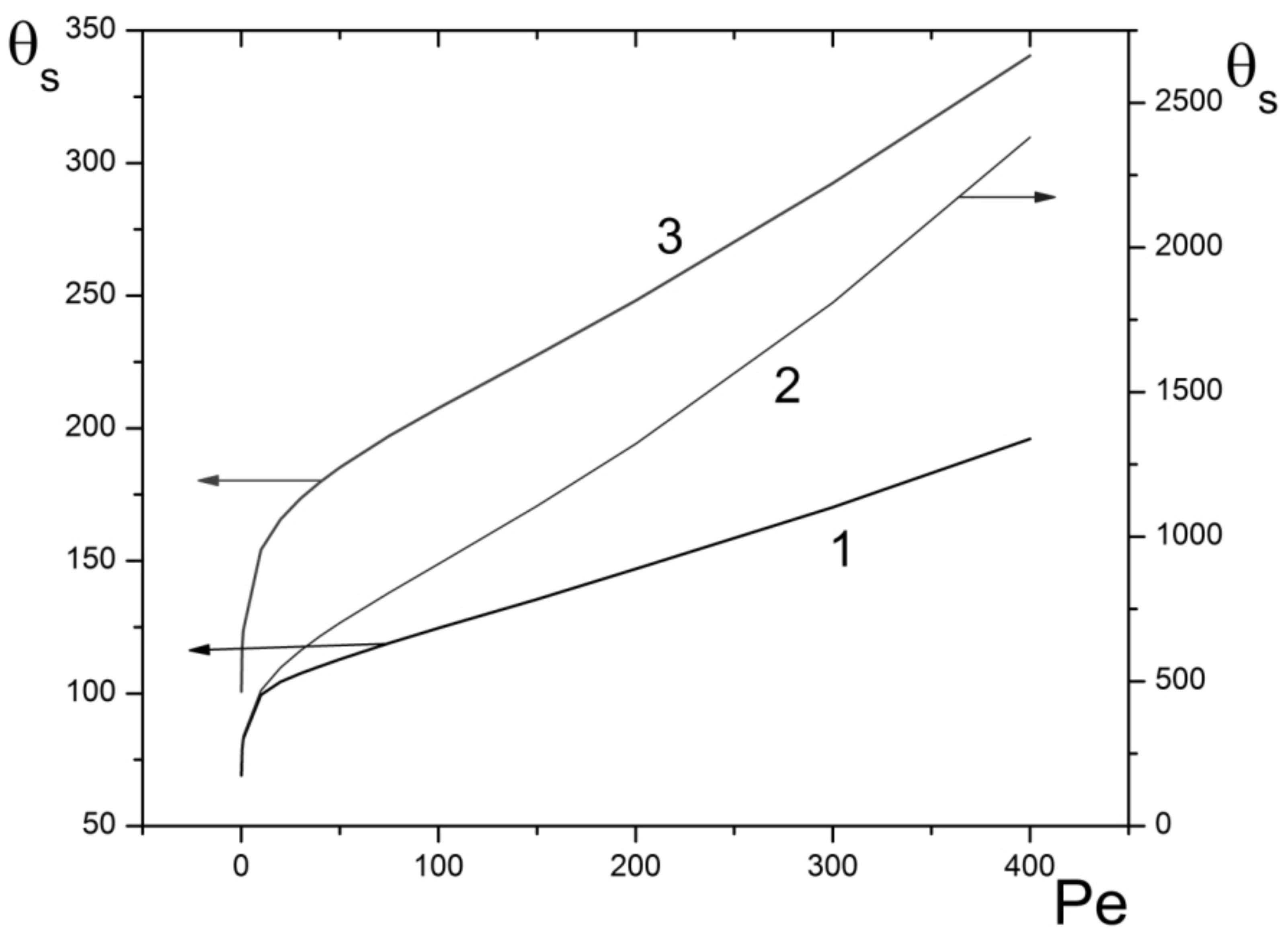
Figure 5 shows three curves drawn at different value of the parameters $A$ and $g$. It is evident that all the three critical curves are monotonic.

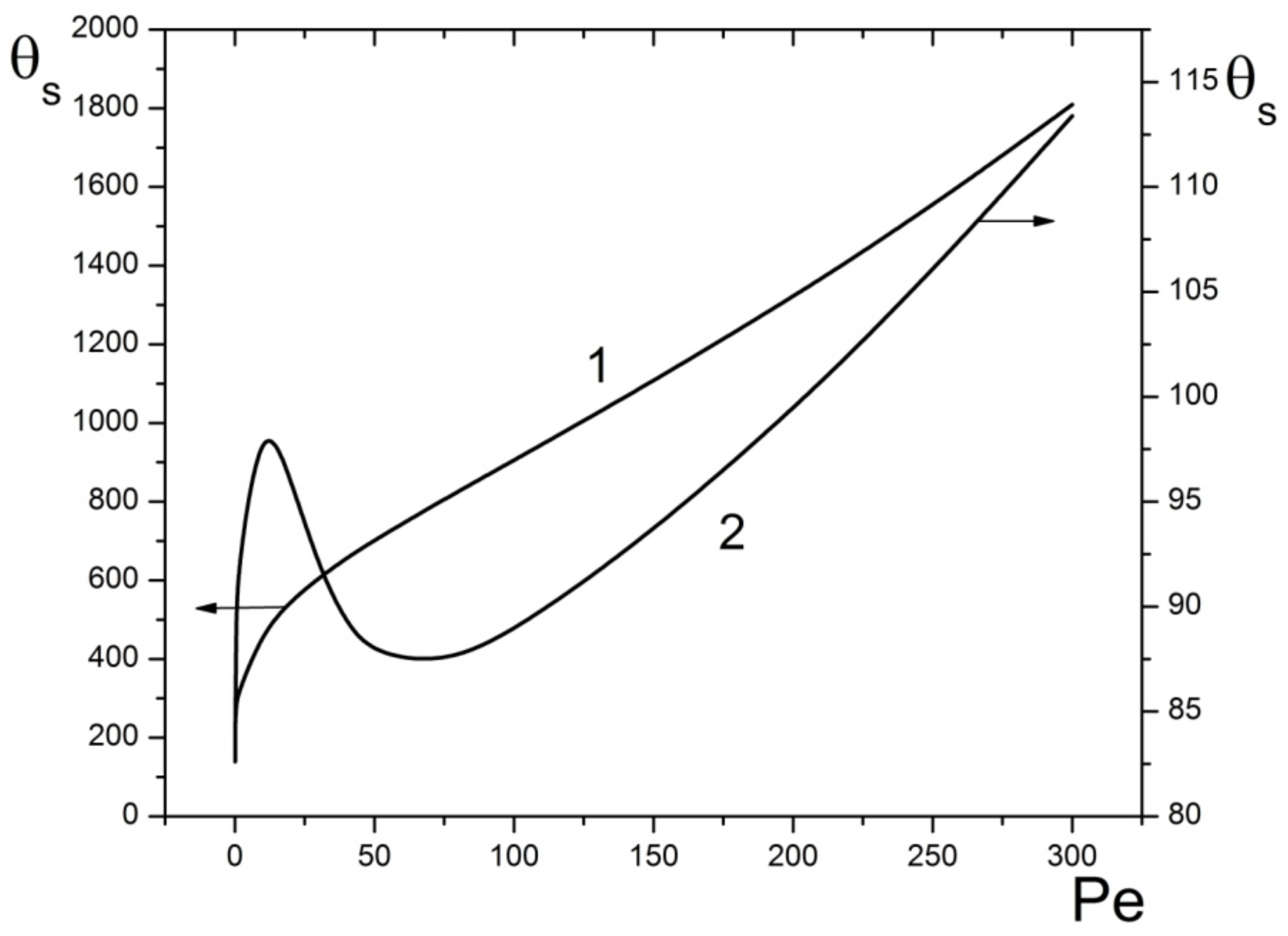
Transition to non-monotonic behavior occurs upon variation of the Arrhenius number $Ar$ (Figure 6), with all other parameters being kept constant. Non-monotonic behavior emerges upon decreasing the Arrhenius number.

The particular type (monotonic or non-monotonic) of the critical curve is controlled by behavior of the integral

$${{\Psi }}_1\left(\xi \right)=\frac{g}{Pe}{\displaystyle \underset{0}{\overset{\xi }{\int }}f\left(\theta \left(s\right)\right)ds}$$

(33)

which must be equal to unity at $\xi =1$.

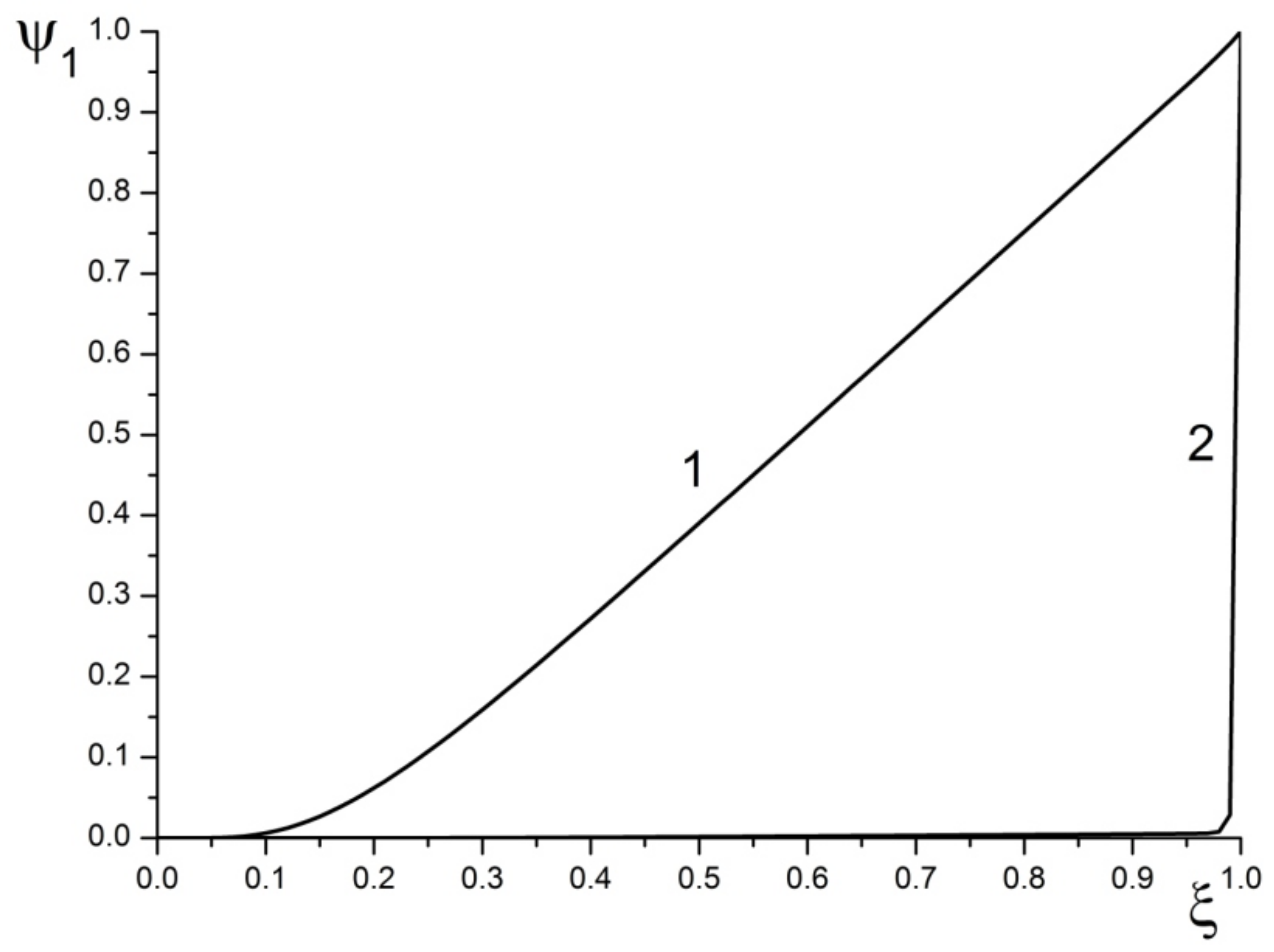
Figure 7 demonstrates these integrals for monotonic and non-monotonic curves. For the non-monotonic solution, the total value of the integral accumulates in the small vicinity of the point $\xi =1$.

In the non-monotonic case (curve 2, Figure 6) the same value of ${\theta }_s=$ 87.70 corresponds to the two values of the parameter $Pe$, namely $Pe=$ 50 and $Pe=$ 84.35.

The solutions $\theta \left(\xi \right)$ for these two values of $Pe$ are presented in Figure 8, while Figure 9 presents the integrals ${{\Psi }}_1\left(\xi \right)$ for these solutions.

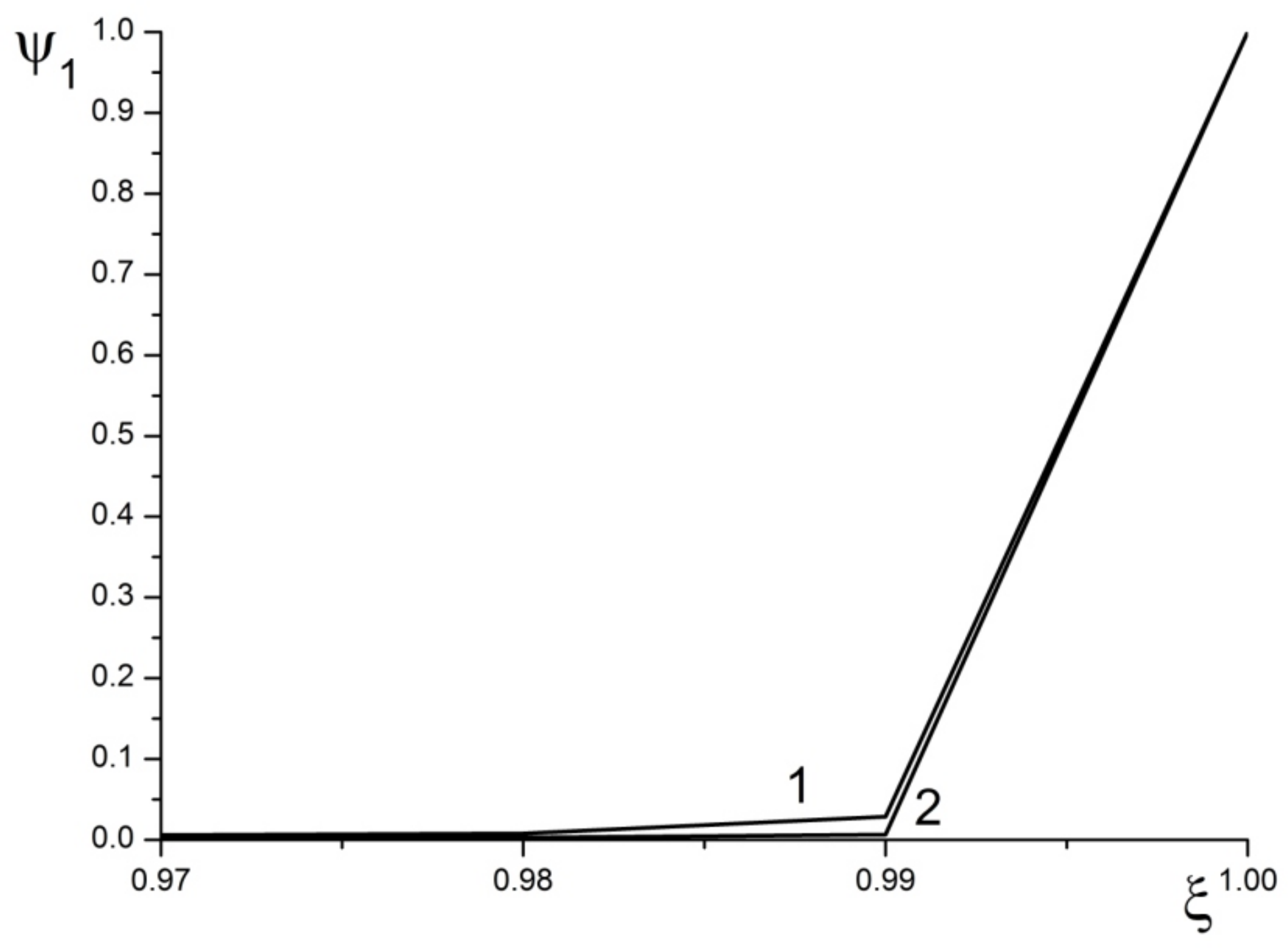
It is evident from Figure 9 that total values of both integrals accumulate in the small vicinity of the point $\xi =1$.

The critical curve decreases at the point ($Pe=$ 50, ${\theta }_s=$ 87.70), and increases at the point ($Pe=$ 84.35, ${\theta }_s=$ 87.70).

It may be concluded that sharp behavior of the integral ${{\Psi }}_1\left(\xi \right)$ in the vicinity of the point $\xi =1$ is the necessary condition for the critical curve to be non-monotonic.

The counterintuitive existence of non-monotonic critical curves may be explained in the following way.

Assuming the approximate $\delta$- function model (29) and setting ${\xi }_0$ = 1 results in the following BVP for the temperature profile on $\left[0,1\right]$

$$\frac{d^2\theta }{d{\xi }^2}-Pe\frac{d\theta }{d\xi }+h_s\left({\theta }_s-\theta \right)=0$$

(34)

$$\theta \left(0\right)=0; \frac{d\theta }{d\xi }\left(1\right)=\mu \cdot Pe$$

and, for a given $Pe$, the value of ${\theta }_s$ is determined from the condition

$$\frac{g}{Pe}{\displaystyle \underset{0}{\overset{1}{\int }}f\left(\theta \left(s\right)\right)ds}=1$$

(35)

where the source function $f\left(\theta \right)$ is given by Equation (5).

Let

$${\lambda }_1=\frac{Pe+\sqrt{P{e}^2+4h_s}}{2}; {\lambda }_2=-\frac{2h_s}{Pe+\sqrt{P{e}^2+4h_s}}$$

(36)

Then ${\lambda }_1$ is sufficiently large for $h_s=$ 720, $Pe<$ 50, while at the same time, ${\lambda }_2$ is negative with sufficiently large absolute value, so that approximately

$$\theta \left(\xi \right)\approx {\theta }_s\left(1-\exp \left({\lambda }_2\xi \right)\right)+\frac{\mu Pe}{{\lambda }_1}\exp \left({\lambda }_1\left(\xi -1\right)\right)$$

(37)

Let us consider the case where the value $\frac{g}{Pe}f\left({\theta }_s\right)$ is negligibly small. It is only in this case when the original problem is well approximated by the model with $\delta$-function source. In this case we can assume

$$\theta \left(\xi \right)={\theta }_s+\frac{\mu Pe}{{\lambda }_1}\exp \left({\lambda }_1\left(\xi -1\right)\right)$$

(38)

and then

$$\frac{d\theta }{d\xi }={\lambda }_1\left(\theta -{\theta }_s\right)$$

(39)

We solve, under the above assumptions, the equation

$$F\left({\theta }_s,Pe\right)=\frac{g}{Pe}{\displaystyle \underset{0}{\overset{1}{\int }}f\left(\theta \left(s\right)\right)ds}=1$$

(40)

with respect to ${\theta }_s$ at a fixed value of $Pe$.

It is easy to see that $F\left({\theta }_s,Pe\right)$ is monotonic with respect to ${\theta }_s$. Therefore, the solution ${\theta }_s\left(Pe\right)$ of the equation $F\left({\theta }_s,Pe\right)=1$ is unique with respect to ${\theta }_s$.

If $\frac{\partial F}{\partial Pe}>0$ at $F\left({\theta }_s,Pe\right)=1$, then $\frac{d{\theta }_s}{dPe}<0$.

Let us calculate $\frac{\partial F}{\partial Pe}$.

Let $u=\theta -{\theta }_s$, then

$$F\left(\theta ,Pe\right)=\frac{g}{Pe}{\displaystyle \underset{1}{\overset{\frac{\mu Pe}{{\lambda }_1}}{\int }}\frac{f\left({\theta }_s+u\right)}{{\lambda }_{1}u}du}$$

(41)

(We assumed that the value $\frac{g}{Pe}f\left({\theta }_s\right)$ is small and the lower bound of the integral is irrelevant).

Further,

$$\begin{array}{l}\frac{\partial F}{\partial Pe}=\frac{2h_s}{{\lambda }_1^2\sqrt{P{e}^2+4h_s}}\frac{\mu g}{Pe}\frac{f\left({\theta }^{\ast }\right)}{\mu Pe}-\\ -\frac{2g}{P{e}^3\sqrt{P{e}^2+4h_s}}{\displaystyle \underset{1}{\overset{\frac{\mu Pe}{{\lambda }_1}}{\int }}\frac{f\left({\theta }_s+u\right)}{u}du=}\\ =\frac{2h_{s}gf\left({\theta }^{\ast }\right)}{{\lambda }_1^{2}P{e}^2\sqrt{P{e}^2+4h_s}}-\frac{2{\lambda }_1}{P{e}^2\sqrt{P{e}^2+4h_s}}\end{array}$$

(42)

Here ${\theta }^{\ast }=\theta \left(1\right)={\theta }_s+\frac{\mu Pe}{{\lambda }_1}$, and we used the fact that

$${\displaystyle \underset{1}{\overset{\frac{\mu Pe}{{\lambda }_1}}{\int }}\frac{f\left({\theta }_s+u\right)}{u}du=}\frac{{\lambda }_{1}Pe}{g}$$

(43)

Therefore, under our assumptions, $\frac{d{\theta }_s}{dPe}<0$ if $f\left({\theta }^{\ast }\right)>\frac{{\lambda }_1^3}{g{h}_s}$.

It is easy to see that upon increasing $\mu$ or decreasing $Ar$ (at fixed $g$, $Pe$, $h_s$), ${\theta }_s\left(Pe\right)$ decreases, while $f\left({\theta }^{\ast }\right)$ increases.

Therefore, by increasing $\mu$ or decreasing $Ar$, we can obtain points on the critical curve where $\frac{d{\theta }_s}{dPe}<0$.

3.4. Comparison with Experimental Data

Let us compare results of the present study with available experimental observations.

Yakovlev et al. [15] conducted a very detailed numerical investigation of flame stabilization process in thin-layered radial porous burner. It consisted of a mounting flange connected with a thin-layered porous shell. Flow configuration for the reported experiment may be considered as a flow through porous wall of the infinitely long hollow cylinder in the direction normal to the wall (i.e., in the plane perpendicular to the axial axis of symmetry of the cylinder). Flow direction is from the inner surface of the cylinder to the outer surface.

Within stable operating ranges, the flame front can be stabilized within the cavity of the burner (internal regime), within porous media (submerged flame) or above it (surface-stabilized flame), by adjusting the equivalence ratio and the flow rate.

The first of these regimes (stabilization upstream from the lattice) is not considered in the present study; however, the latter two are of most interest. Similar to the present study, Yakovlev et al. [15] observed two types of temperature distribution profiles, that is monotonic and non-monotonic. When the flame stabilized within porous media (submerged regime), then a non-monotonic profile was observed. When the flame stabilized downstream from the surface (surface-stabilized regime), then a monotonic profile was observed. This change of profile configuration upon flame front relocating from the porous to the gas region is quantitatively identical to the behavior reported in Figure 2 and Figure 3 of the present study.

Mital et al. [17] and Janvekar et al. [27] considered porous burners of cylindrical shape, with the flow parallel to the to the axial axis of symmetry of the cylinder. This configuration would be asymptotically identical to the one used in the present study if the radius of the cylinder increases infinitely.

Both studies observed the flame stabilization regime inside the porous material (submerged reaction zone) with non-monotonic temperature profiles similar the one presented in Figure 2.

Thus, the studies of Yakovlev et al. [15], Mital et al. [17], Janvekar et al. [27] and Keshtkar et al. [34] provide indirect, but nevertheless very convincing support for the results of the present study.

4. Conclusions

The standing premixed combustion wave on a lattice burner has two qualitatively distinctive regimes: flame stabilizes either downstream from the burner surface or inside the solid lattice.

For the first time, this fact has been proved absolutely rigorously using a one-dimensional analytical model of reacting flow.

It has also been demonstrated using numerical simulations.

In the space of controlling parameters, the two stabilization regimes are separated by the specific dependence of the lattice temperature on the flow Peclet number (the critical curve), with all other parameters being fixed.

Transition from monotonic to non-monotonic regimes occurs as the Arrhenius number sufficiently decreases.

Results of the present study agree qualitatively with the available experimental data.

Novelties of the present study may be summarized as follows: a new model of the standing combustion wave stabilized on a lattice (porous) burner is proposed. The model allows for qualitative analytical investigation of the problem to be performed. An approximated model, based on description of chemical source term with $\delta$-function, is also developed. The exact analytical solution is obtained for this model. Rigorous mathematical proof of existence of the two distinctive combustion wave modes, with monotonic and non-monotonic temperature profiles, respectively, is demonstrated for the first time. Definition of critical curve in the space of control parameters, separating the two combustion wave modes, is proposed. Rigorous mathematical proof of existence of both monotonic and non-monotonic critical curves is demonstrated.

In terms of quantitative results, proposed analytical model, based on $\delta$-function approximation of chemical source term, agrees well (within 7% relative error) with the model based on distributed description of chemical reaction zone.

The proven existence of the two significantly different combustion regimes is of great practical importance and impacts design solutions for industrial porous burners. The results will be of great interest to the broader academic community, particularly in research areas where similar wave structures may emerge.

References

- Williams, F.A. Combustion Theory; CRC Press: Boca Raton, FL, USA, 2018. [Google Scholar]
- Kuo, K.K. Principles of Combustion; Wiley: Hoboken, NJ, USA, 2005. [Google Scholar]
- Zeldovich, Y.B.; Barenblatt, G.I.; Librovich, V.B.; Makhviladze, G.M. Mathematical Theory of Combustion and Explosion; Nauka: Moscow, Russia, 1980. (In Russian) [Google Scholar]
- Merzhanov, A.G.; Khaikin, B.I. Theory of Combustion Waves in Homogeneous Media. Prog. Energy Combust. Sci. 1988, 14, 1–98. (In Russian) [Google Scholar] [CrossRef]
- Novozhilov, B.V.; Novozhilov, V.B. Theory of Solid-Propellant Nonsteady Combustion; Wiley-ASME Press: Hoboken, NJ, USA, 2021. [Google Scholar]
- Merzhanov, A.G. Self-propagating high-temperature synthesis: Twenty years of search and findings. In Combustion and Plasma Synthesis of High-Temperature Materials; Munir, Z.A., Holt, J.B., Eds.; VCH: Vancouver, BC, Canada, 1990; pp. 1–53. [Google Scholar]
- Hirano, T.; Saito, K. Fire Spread Phenomena: The Role of Observation in Experiment. Prog. Energy Combust. Sci. 1994, 20, 461–485. [Google Scholar] [CrossRef]
- Fernandez-Pello, A.C.; Hirano, T. Controlling Mechanisms of Flame Spread. Combust. Sci. Technol. 1983, 32, 1–31. [Google Scholar] [CrossRef]
- Smirnov, N.N.; Dimitrienko, I.D. Convective Combustion of Porous Compressible Propellants. Combust. Flame 1992, 89, 260–270. [Google Scholar] [CrossRef]
- Aldushin, A.P.; Matkowsky, B.J.; Schult, D.A.; Shkadinskaya, G.V.; Shkadinsky, K.G.; Volpert, V.A. Porous medium combustion. In Modeling in Combustion Science; Lecture Notes in Physics; Buckmaster, J., Takeno, T., Eds.; Springer: Berlin/Heidelberg, Germany, 1995; Volume 449. [Google Scholar] [CrossRef]
- Aldushin, A.P.; Seplyarsky, B.S. Propagation of waves of exothermal reaction in porous medium during gas blow-through. Sov. Phys. Dokl. 1978, 23, 483–485. [Google Scholar]
- Shkadinsky, K.G.; Shkadinskaya, G.V.; Matkowsky, B.J.; Volpert, V.A. Two front traveling waves in filtration combustion. SIAM J. Appl. Math. 1993, 53, 128–140. [Google Scholar] [CrossRef]
- Schult, D.A.; Matkowsky, B.J.; Volpert, V.A.; Fernandez-Pello, A.C. Propagation and Extinction of Forced Opposed Flow Smolder Waves. Comb. Flame 1995, 101, 471–490. [Google Scholar] [CrossRef]
- Wahle, C.W.; Matkowsky, B.J. Rapid, Upward Buoyant Filtration Combustion Waves Driven by Convection. Combust. Flame 2001, 124, 14–34. [Google Scholar] [CrossRef]
- Yakovlev, I.; Maznoy, A.; Zambalov, S. Pore-scale Study of Complex Flame Stabilization Phenomena in Thin-layered Radial Porous Burner. Combust. Flame 2021, 231, 111468. [Google Scholar] [CrossRef]
- Sangjukta, D.; Sahoo, N.; Muthukumar, P. Experimental Studies on Biogas Combustion in a Novel Double Layer Inert Porous Radiant Burner. Renew. Energy 2020, 149, 1040–1052. [Google Scholar]
- Mital, R.; Gore, J.P.; Viskanta, R. A Study of the Structure of Submerged Reaction Zone in Porous Ceramic Radiant Burners. Combust. Flame 1997, 111, 175–184. [Google Scholar] [CrossRef]
- Fursenko, R.; Maznoy, A.; Odintsov, E.; Kirdyashkin, A.; Minaev, S.; Sudarshan, K. Temperature and Radiative Characteristics of Cylindrical Porous Ni–Al Burners. Int. J. Heat Mass Transf. 2016, 98, 277–284. [Google Scholar] [CrossRef]
- Ferguson, J.C.; Sobhani, S.; Ihme, M. Pore-resolved Pimulations of porous Media Combustion with Conjugate Heat Transfer. Proc. Combust. Inst. 2021, 38, 2127–2134. [Google Scholar] [CrossRef]
- Bedoya, C.; Dinkov, I.; Habisreuther Zarzalis, P.N.; Bockhorn, H.; Parthasarathy, P. Experimental study, 1D Volume-averaged Calculations and 3D Direct Pore Level Simulations of the Flame Stabilization in Porous Inert Media at Elevated Pressure. Combust. Flame 2015, 162, 3740–3754. [Google Scholar] [CrossRef]
- Sirotkin, F.; Fursenko, R.; Kumar, S.; Minaev, S. Flame Anchoring Regime of Filtrational Gas Combustion: Theory and Experiment. Proc. Combust. Inst. 2017, 36, 4383–4389. [Google Scholar] [CrossRef]
- Yakovlev, I.; Zambalov, S. Three-dimensional Pore-scale Numerical Simulation of Methane-air Combustion in Inert Porous Media under the Conditions of Upstream and Downstream Combustion Wave Propagation through the Media. Combust. Flame 2019, 209, 74–98. [Google Scholar] [CrossRef]
- Billerot, P.-L.; Dufresne, L.; Lemaire, R.; Seers, P. 3D CFD Analysis of a Diamond Lattice-based Porous Burner. Energy 2020, 207, 118–160. [Google Scholar] [CrossRef]
- Wood, S.; Harris, A.T. Porous Burners for Lean-burn Applications. Prog. Energy Combust. Sci. 2008, 34, 667–684. [Google Scholar] [CrossRef]
- Wua, C.-Y.; Chen, K.-H.; Yang, S.Y. Experimental Study of Porous Metal Burners for Domestic Stove Applications. Energy Convers. Manag. 2014, 77, 380–388. [Google Scholar] [CrossRef]
- Dehaj, M.S.; Ebrahimi, R.; Shams, M.; Farzaneh, M. Experimental Analysis of Natural Gas Combustion in a Porous Burner. Exp. Therm. Fluid Sci. 2017, 84, 134–143. [Google Scholar] [CrossRef]
- Janvekar, A.A.; Miskam, M.A.; Abas, A.; Ahmad, Z.A.; Juntakan, T.; Abdullah, M.Z. Effects of the Preheat Layer Thickness on Surface/Submerged Flame during Porous Media Combustion of Micro Burner. Energy 2017, 122, 103–110. [Google Scholar] [CrossRef]
- Gao, H.B.; Qu, Z.G.; Feng, X.B.; Tao, W.Q. Methane/Air Premixed Combustion in a Two-layer Porous Burner with Different Foam Materials. Fuel 2014, 115, 154–161. [Google Scholar] [CrossRef]
- Al-attab, K.A.; Ho, J.C.; Zainal, Z.A. Experimental Investigation of Submerged Flame in Packed Bed Porous, Media Burner Fueled by Low Heating Value Producer Gas. Exp. Therm. Fluid Sci. 2015, 62, 1–8. [Google Scholar] [CrossRef]
- Bouma, P.H.; De Goey, L.P.H. Premixed Combustion on Ceramic Foam Burners. Combust. Flame 1999, 119, 133–143. [Google Scholar] [CrossRef]
- Barra, A.J.; Diepvens, G.; Ellzey, J.L.; Henneke, M.R. Numerical Study of the Effects of Material Properties on Flame Stabilization in a Porous Burner. Combust. Flame 2003, 134, 369–379. [Google Scholar] [CrossRef]
- Barra, A.J.; Ellzey, J.L. Heat Recirculation and Heat Transfer in Porous Burners. Combust. Flame 2004, 137, 230–241. [Google Scholar] [CrossRef]
- Lari, K.; Gandjalikhan Nassab, S.A. Transient Thermal Characteristics of Porous Radiant Burners. Iran. J. Sci. Technol. 2007, 31, 407–420. [Google Scholar]
- Keshtkar, M.M.; Gandjalikhan Nassab, S.A. Theoretical Analysis of Porous Radiant Burners under 2-D Radiation Field Using Discrete Ordinates Method. J. Quant. Spectrosc. Radiat. Transf. 2009, 110, 1894–1907. [Google Scholar] [CrossRef]
- Djordjevic, N.; Habisreuther, P.; Zarzalis, N. A Numerical Investigation of the Flame Stability in Porous Burners Employing Various Ceramic Sponge-like Structures. Chem. Eng. Sci. 2011, 66, 682–688. [Google Scholar] [CrossRef]
- Arutyunov, V.S.; Belyaev, A.A.; Lidskii, B.V.; Nikitin, A.V.; Posvyanskii, V.S.; Shmelev, V.M. Numerical Solution of the Problem of Surface Combustion on Flat Porous Matrix. AIP Conf. Proc. 2018, 2046, 020075. [Google Scholar] [CrossRef]
- Shmelev, V.M. Combustion of a Mixed Mixture in a Slot Matrix. Russ. J. Phys. Chem. B 2020, 14, 670–677. [Google Scholar] [CrossRef]
- Godunov, S.K.; Ryaben’kii, V.S. Difference Schemes; North Holland: Amsterdam, The Netherlands, 1987. [Google Scholar]
- Incropera, F.P.; DeWitt, D.P. Fundamentals of Heat and Mass Transfer; Wiley: Hoboken, NJ, USA, 2002. [Google Scholar]
- Borman, G.L.; Ragland, K.W. Combustion Technology; McGraw-Hill: New York, NY, USA, 1998. [Google Scholar]
Figure 1.
Schematic of the lattice burner considered: (a) side view (cross-section) and (b) front (upstream) view.
Figure 2.
Non-monotonic solutions. 1—approximate model (29); 2—original model (5). Pe = 135; A = 2.75 × 10⁻¹⁸; Ar = 0.012; hs = 7.14 × 10²; = 90; g = 1.0 × 10⁻²⁰; = 91.67; = 0.41.
Figure 3.
Monotonic solutions. 1—approximate model (29); 2—original model (5); Pe = 135; A = 2.75 × 10⁻¹⁸; Ar = 0.012; hs = 7.14 × 10²; = 50; g = 1.0 × 10⁻²⁰; = 91.67; = 1.74.
Figure 4.
Critical curve . 1—approximate model (29); 2—original model (5); A = 2.75 × 10⁻¹⁸; Ar = 0.012; hs = 7.14 × 10²; g = 1.0 × 10⁻²⁰; = 91.67.
Figure 5.
Monotonic critical curves. Approximate model (29). Ar = 0.02; hs = 7.14 × 10²; = 75.0; 1—A = 2.75 × 10⁻¹³; g = 1.22 × 10⁻¹⁵; 2—A = 2.75 × 10⁻¹⁵; g = 1.22 × 10⁻¹⁷; 3—A = 2.75 × 10⁻¹⁸; g = 1.22 × 10⁻²⁰.
Figure 6.
Transition from monotonic to non-monotonic critical curve. Approximate model (29). A = 2.75 × 10⁻¹⁸; hs = 7.14 × 10²; = 75.0; g = 1.22 × 10⁻²⁰, 1—Ar = 0.02, 2—Ar = 0.012.
Figure 7.
The integral . Approximate model (29). A = 2.75 × 10⁻¹⁸; hs = 7.14 × 10²; = 75.0; g = 1.22 × 10⁻²⁰. 1—monotonic critical curve. Ar = 0.02; Pe = 50.0; = 702.01. 2—non-monotonic critical curve. Ar = 0.012; Pe = 50.0; = 87.70.
Figure 8.
Solutions in the case of non-monotonic critical curve. Approximate model (29). A = 2.75 × 10⁻¹⁸; Ar = 0.012; hs = 7.14 × 10²; = 75.0; g = 1.22 × 10⁻²⁰; = 87.70; 1—Pe = 50.0; 2—Pe = 84.35.
Figure 9.
The integrals for the Figure 8 solutions. Approximate model (29). A = 2.75 × 10⁻¹⁸; Ar = 0.012; hs = 7.14 × 10²; = 75.0; g = 1.22 × 10⁻²⁰; = 87.70; 1—Pe = 50.0; 2—Pe = 84.35.
Publisher’s Note: MDPI stays neutral with regard to jurisdictional claims in published maps and institutional affiliations. |
© 2022 by the authors. Licensee MDPI, Basel, Switzerland. This article is an open access article distributed under the terms and conditions of the Creative Commons Attribution (CC BY) license (https://creativecommons.org/licenses/by/4.0/).
Share and Cite
MDPI and ACS Style
Novozhilov, V.B.; Lidskii, B.V.; Posvyanskii, V.S. Different Modes of Combustion Wave on a Lattice Burner. Mathematics 2022, 10, 2731. https://0-doi-org.brum.beds.ac.uk/10.3390/math10152731
AMA Style
Novozhilov VB, Lidskii BV, Posvyanskii VS. Different Modes of Combustion Wave on a Lattice Burner. Mathematics. 2022; 10(15):2731. https://0-doi-org.brum.beds.ac.uk/10.3390/math10152731
Chicago/Turabian StyleNovozhilov, Vasily B., Boris V. Lidskii, and Vladimir S. Posvyanskii. 2022. "Different Modes of Combustion Wave on a Lattice Burner" Mathematics 10, no. 15: 2731. https://0-doi-org.brum.beds.ac.uk/10.3390/math10152731
Note that from the first issue of 2016, this journal uses article numbers instead of page numbers. See further details here.