
Improved Stability Criteria for Delayed Neural Networks via a Relaxed Delay-Product-Type Lapunov–Krasovskii Functional


1
School of Computer, Chengdu University, Chengdu 610106, China
2
School of Electronic Information and Electrical Engineering, Chengdu University, Chengdu 610106, China
3
School of Aeronautics and Astronautics, University of Electronic Science and Technology of China, Chengdu 611731, China
*
Author to whom correspondence should be addressed.
Mathematics 2022, 10(15), 2768; https://0-doi-org.brum.beds.ac.uk/10.3390/math10152768
Submission received: 14 July 2022
/
Revised: 31 July 2022
/
Accepted: 2 August 2022
/
Published: 4 August 2022
(This article belongs to the Special Issue Well-Posedness, Dynamics, and Control of Nonlinear Differential System with Initial-Boundary Value)
Abstract
:In this paper, the asymptotic stability problem of neural networks with time-varying delays is investigated. First, a new sufficient and necessary condition on a general polynomial inequality was developed. Then, a novel augmented Lyapunov–Krasovskii functional (LKF) was constructed, which efficiently introduces some new terms related to the previous information of neuron activation function. Furthermore, based on the suitable LKF and the stated negative condition of the general polynomial, two criteria with less conservatism were derived in the form of linear matrix inequalities. Finally, two numerical examples were carried out to confirm the superiority of the proposed criteria, and a larger allowable upper bound of delays was achieved.
Keywords:
neural networks; asymptotic stability; polynomial inequalities; time-varying delays; Lyapunov–Krasovskii functional (LKF)MSC:
93D201. Introduction
Neural networks (NNs) are generally recognized as one of the mathematical models that simulates the intelligent activities of the human brain [1]. Because of its strong ability to model complex and nonlinear relationships between the input and output, NNs have attracted widespread attention over the past decades and have been applied in many areas, such as image processing [2], optimization problems [3], signal processing [4], parallel computation [5] and other scientific fields. However, due to the limited switching frequency of amplifiers and the inherent communication time among neurons, time delays are inevitable, which may affect the performance of NNs and lead to undesired dynamics, such as oscillation or even instability [6,7,8]. Therefore, it is essential to consider an allowable upper bound of delays such that the NNs with a delay less than this bound remain stable, and many excellent results have been achieved to reduce the conservatism of the stability conditions [9,10,11,12].
It is well recognized that the Lyapunov–Krasovskii functional (LKF) method is powerful in analyzing such delayed NNs. The key point is concerned with the choice of LKF [13,14]. It has been verified that an LKF with delay-dependent matrices can yield less conservatism. A delay-product-type LKF is proposed in [15], which contains a matrix-valued polynomial of any chosen degree in time-varying delay. It shows that the conservatism is affected by the maximal degree of time-varying delay included in the delay-product-type terms of the LKF. Additionally, by taking into consideration more information on state-related vectors and the activation function, some newly augmented LKFs are presented in [13,14,16,17]. As a result, less conservative conditions are predicted, as more information about the state, delay or neuron activation functions are beneficial for reducing conservatism. Therefore, one of the research contents of this work is to build a delay-product-type LKF that contains more information on state-related vectors and the activation function, and hence is able to lead to a less conservative stability criterion.
Besides the construction of a proper LKF, the estimation of an integral term originating in the derivative of LKF is strongly related to the conservatism of criteria [18]. A common term with the form is always included in different LKFs. Then, its derivative contains the term as follows: . Various integral inequalities techniques have been proposed to bound such integral terms. The Jensen inequality [19] is known as an efficient tool to estimate the integral terms, but the reciprocally convex combination terms are usually encountered with respect to the time-varying delays, and the reciprocally convex lemma must be used to handle them [20,21]. Based on this work, many researchers have focus on the investigation of novel integral inequalities to obtain less conservative results of stability for the systems. Wirtinger-based integral inequality is investigated in [18], which encompasses Jensen inequality and obtains better results than Jensen inequality. Free-matrix-based integral inequality with a tighter bound has been proposed, while the reciprocally convex lemma is no longer required, but this increased the computational complexity [22]. Several zero-value equalities that add cross terms to the time derivative LKF terms are proposed, and improved results are derived. A novel estimating method called the general free-weighting-matrix approach is created in [17]. It is shown that this approach can incorporate Wirtinger-based inequality and free-matrix-based integral inequality. It has to be pointed out that the construction of an LKF should take integral inequalities into account to ensure that the derivative of the LKF includes those vectors appearing in the integral inequality used [23]. Therefore, utilizing a valid integral inequality technique to bound the integral terms is strongly connected with the conservatism of stability criteria. This paper investigates the stability of NNs following this direction.
In this paper, we further investigate the stability problem for NNs with time-varying delays. The contributions of this paper are summarized as follows:
- (i)
- A new sufficient and necessary condition for the general polynomial inequalities was developed by introducing some slack variables. The negative definiteness determination method was applied to derive less conservative stablity criteria.
- (ii)
- A suitable delay-product-type LKF was constructed by efficiently introducing some new terms relating to the previous information of neuron activation function. As a result, the stability criterion based on the established LKF becomes more dependent on the technique for dealing with the single integrations of activation function.
- (iii)
- Based on the LKF and the stated negative condition of the general polynomial, two less conservative criteria were derived, which are demonstrated through two numerical examples, and a larger allowable upper bound of delays is achieved.
Notations: Throughout this paper, represents the set of positive integers. and denote the n-dimensional vector space and the set of all real matrices, respectively. and stand for the inverse and the transpose of the matrix Z, respectively. () means that P is a symmetric and positive definite (semi-definite) matrix. I and 0 denote the identity matrix and zero matrix. represents a diagonal matrix, in which, its diagonal elements are . , . ∗ stands for the symmetric terms in a symmetric matrix. represents .
2. Preliminaries
In this section, we consider the following NNs system:
where denotes the neuron state vector and is a diagonal matrix. and are the interconnection weight matrices, and is the activation function with . The time-varying delay satisfies
where h and are known positive constants. The neuron activation function is bounded by
where and are real scalars. For convenience, define , .
In order to derive the stability criteria for the system (1), the following lemmas were utilized.
Lemma 1
([24]). For an integer , two scalars a and b with , a real positive matrix R and a differentiable function such that the integration below is well defined, then
where ,
, .
Lemma 2
Lemma 3
([25]). Consider an integrable function in , and a matrix T with appropriate dimensions. The following inequality is true.
where β is an arbitrary vector, and .
Lemma 4.
Consider the following polynomial described by , where , with h is a constant; then,
- (i)
- for all if and only if there exists a scalar such thatwhere , and .
- (ii)
- for all if and only if there exists a scalar such thatwhere , and .
Proof.
(i) First, for , we define . and can be represented as and , respectively.
(Sufficiency) If there exists a scalar satisfying , then for all .
(Necessity) is a convex set. Then, we set an open convex cone as . If there exists a nonzero two-tuple , we have
For any given , we have , for all . Thus, (11) implies that . Since is regular, (12) shows that . Hence, the following inequality can be obtained by using :
for . This means that there exists such that . This completes the proof of (i).
(ii) Set ; then, can be rewritten as , where
Then, the proof is straightforward from the proof of (i). □
Remark 1.
Lemma 4 provides necessary and sufficient conditions of high-order polynomial inequality and for . When represents an odd polynomial on z if . Thus, Lemma 4 covers both even and odd polynomials. It is worth mentioning that Lemma 2 in [26] is a special case of Lemma 4 with . A quadratic function for all if and only if there exists a scalar such that
3. Main Results
In this section, two improved stability criteria are developed. For simplification, the following notations are defined.
- ,
- ,
Now, we present the following stability conditions.
Theorem 1.
For given scalars and , the system (1) is asymptotically stable if there exist symmetric matrices , diagonal matrices and any matrices , such that
where , with
Proof.
Based on Lemmas 1 and 2, it follows from (14) that
Using Lemma 3, one has the following inequality:
To make use of the information of the activation function, we can obtain
where ; then, it is clear that
Remark 2.
To derive the stability criterion in terms of linear matrix inequality, the matrix should be appropriately designed. In Theorem 1, are set as to handle and of Ω. The slack variable helps in reducing the conservativeness by giving the freedom for checking the feasibility of the linear matrix inequality conditions.
Remark 3.
It should be pointed out that most literature [11,28] only propose the information of activation functions, such as and . In this paper, the information of single integrations of activation functions, i.e., and , are considered in . According to this construction, more activation function information on NNs can be adequately utilized, which leads to less conservative results. is firstly proposed in [11]; different from its derivative handled method, this paper estimates the integral term by Lemma 3, which makes full use of cross-terms from the single integrations of activation function to others, and leads to a tighter bound.
Corollary 1.
For given scalars and , the system (1) is asymptotically stable if there exist symmetric matrices , diagonal matrices and any matrices , such that
where
where the other notions are defined well in Theorem 1.
Proof.
From the proof of Theorem 1, we choose the LKF (19) with in . The rest of the process is similar to that in the proof of Theorem 1; hence, we omit it here. □
4. Illustrative Examples
In this section, two numerical examples are presented to demonstrate the superiority and the effectivity of the derived criteria.
Example 1.
Consider the delayed NNs (1) with the following parameters:
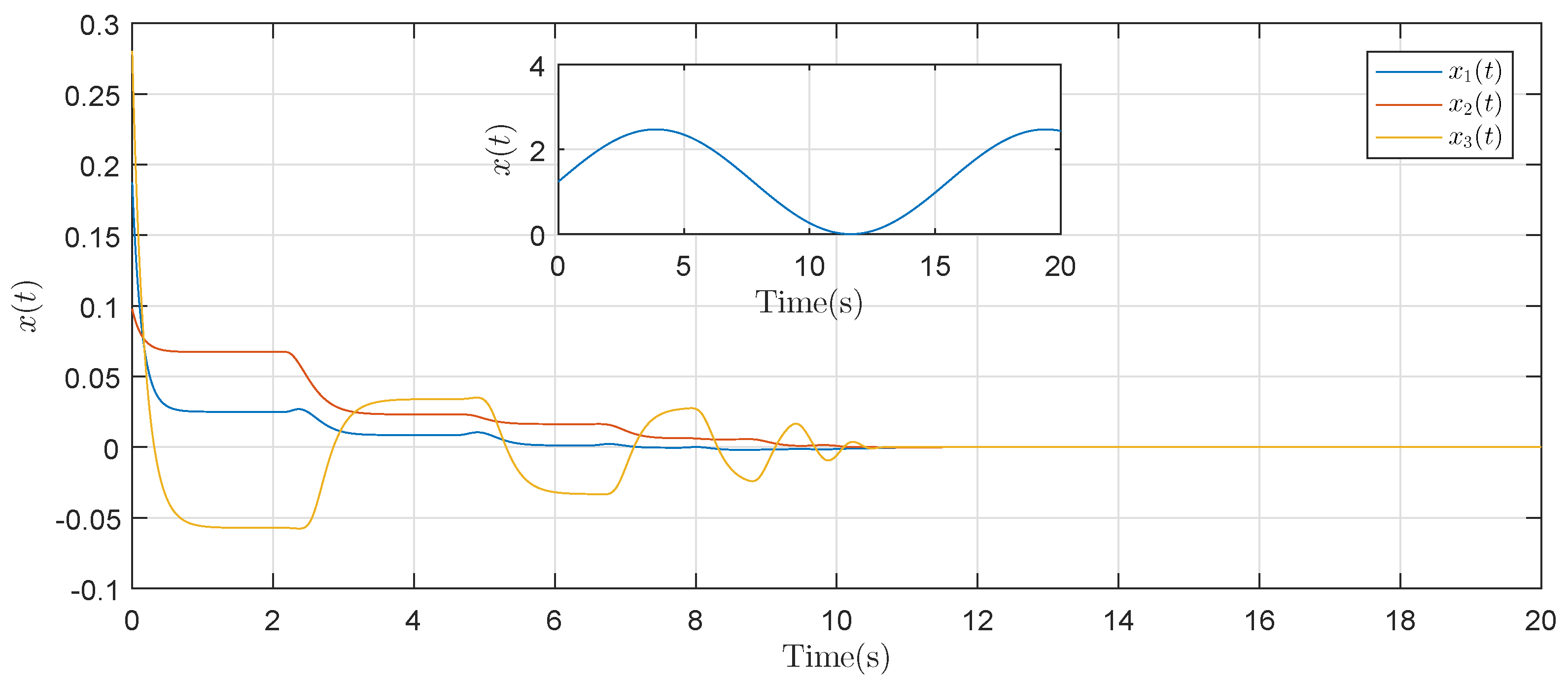
For various , the allowable maximum delay bounds by Theorem 1 and Corollary 1 in this paper and the related methods in [17,32,33,34] are listed in Table 1. The results show that Theorem 1 provides a bigger allowable maximum upper bound of delays than the related methods of [17,32,33,34] do, which verifies the lower conservatism of the proposed criteria. Theorem 1 and Corollary 1 are derived via a similar approach; it can be seen that Theorem 1 provides larger allowable upper delay bounds than Corollary 1, which means that the LKF that contains delay-dependent matrices can lead to a less conservative result. In addition, when , the initial state and . The state trajectories of the given in Figure 1 show that the NNs (1) are stable at their equilibrium points, which verifies the effectiveness of our methods.
Example 2.
Consider the delayed NNs (1) with the following parameters:
It can be easily found that the proposed stability criteria can produce a larger allowable maximum upper bound for all cases than those given in the existing literature. This shows that the proposed criteria are indeed less conservative than the ones in the literature. Table 2 shows the allowable maximum upper bound of delays for various . When , the initial state , and the activation function ; the state trajectories of NNs in Example 2 are shown in Figure 2. The results given reveal that the LKF with a more integral term of activation function (i.e., and ) has improved the results.
5. Conclusions
This paper has investigated the stability problem of NNs with time-varying delays. A positivity and negativity definiteness condition for a general polynomial with any chosen degree in time-varying delay has been established and a relaxed LKF that includes more previous information of the neuron activation function has been proposed. Benefiting from the relaxed LKF and the negative definiteness determination method, two stability criteria with less conservatism have been derived, which has been demonstrated by two numerical examples. Nevertheless, the definiteness condition is still proposed with conservatism, and future work on reducing its conservatism is meaningful.
Author Contributions
Conceptualization, S.W. and K.S.; formal analysis, S.W. and K.S.; funding acquisition, K.S.; methodology, S.W., K.S. and J.Y.; project administration, K.S.; software, S.W.; supervision, K.S.; validation, S.W. and J.Y.; visualization, S.W. and J.Y.; writing—original draft, S.W.; writing—review and editing, K.S. and J.Y. All authors have read and agreed to the published version of the manuscript.
Funding
This work was supported by the National Natural Science Foundation of China under Grant (No. 61703060 and 12061088), the Sichuan Science and Technology Program under Grant No. 21YYJC0469, the Project funded by China Postdoctoral Science Foundation under Grant Nos. 2020M683274 and 2021T140092, Central Government Funds of Guiding Local Scientific and Technological Development for Sichuan Province of China under grant 2021ZYD0012, the Opening Fund of Geomathematics Key Laboratory of Sichuan Province (scsxdz2020zd01).
Institutional Review Board Statement
Not applicable.
Informed Consent Statement
Not applicable.
Data Availability Statement
Not applicable.
Conflicts of Interest
The authors declare no conflict of interest.
References
- Lee, T.H.; Park, M.J.; Park, J.H. An improved stability criterion of neural networks with time-varying delays in the form of quadratic function using novel geometry-based conditions. Appl. Math. Comput. 2021, 404, 126–226. [Google Scholar] [CrossRef]
- Chua, L.; Yang, L. Cellular neural networks: Applications. IEEE Trans. Circuits Syst. 1988, 35, 1273–1290. [Google Scholar] [CrossRef]
- Mestari, M.; Benzirar, M.; Saber, N.; Khouil, M. Solving Nonlinear Equality Constrained Multiobjective Optimization Problems Using Neural Networks. IEEE Trans. Neural Netw. Learn. Syst. 2015, 26, 2500–2520. [Google Scholar] [CrossRef]
- Zhang, H.; Wang, Z.; Liu, D. A Comprehensive Review of Stability Analysis of Continuous-Time Recurrent Neural Networks. IEEE Trans. Neural Netw. Learn. Syst. 2014, 25, 1229–1262. [Google Scholar] [CrossRef]
- Chen, Y.H.; Fang, S.C. Neurocomputing with time delay analysis for solving convex quadratic programming problems. IEEE Trans. Neural Netw. Learn. Syst. 2000, 11, 230–240. [Google Scholar] [CrossRef] [PubMed]
- Melin, P.; Castillo, O. An intelligent hybrid approach for industrial quality control combining neural networks, fuzzy logic and fractal theory. Inf. Sci. 2007, 177, 1543–1557. [Google Scholar] [CrossRef]
- Melin, P.; Mendoza, O.; Castillo, O. Face Recognition With an Improved Interval Type-2 Fuzzy Logic Sugeno Integral and Modular Neural Networks. IEEE Trans. Syst. Man Cybern. A Syst. Hum. 2011, 41, 1001–1012. [Google Scholar] [CrossRef]
- Melin, P.; Sánchez, D.; Castillo, O. Genetic optimization of modular neural networks with fuzzy response integration for human recognition. Inf. Sci. 2012, 197, 1–19. [Google Scholar] [CrossRef]
- Zhang, X.M.; Han, Q.L.; Ge, X.; Ding, D. An overview of recent developments in Lyapunov–Krasovskii functionals and stability criteria for recurrent neural networks with time-varying delays. Neurocomputing 2018, 313, 392–401. [Google Scholar] [CrossRef]
- Zhang, X.M.; Han, Q.L.; Ge, X. An overview of neuronal state estimation of neural networks with time-varying delays. Inf. Sci. 2019, 478, 83–99. [Google Scholar] [CrossRef]
- Chen, J.; Park, J.H.; Xu, S. Stability Analysis for Delayed Neural Networks With an Improved General Free-Matrix-Based Integral Inequality. IEEE Trans. Neural Netw. Learn. Syst. 2020, 31, 675–684. [Google Scholar] [CrossRef]
- Xu, B.; Li, B. Event-Triggered State Estimation for Fractional-Order Neural Networks. Mathematics 2022, 10, 325. [Google Scholar] [CrossRef]
- Kwon, O.M.; Park, M.J.; Lee, S.M.; Park, J.H.; Cha, E.J. Stability for Neural Networks With Time-Varying Delays via Some New Approaches. IEEE Trans. Neural Netw. Learn. Syst. 2013, 24, 181–193. [Google Scholar] [CrossRef]
- Zhang, X.M.; Han, Q.L. Global Asymptotic Stability for a Class of Generalized Neural Networks with Interval Time-Varying Delays. IEEE Trans. Neural Netw. Learn. Syst. 2011, 22, 1180–1192. [Google Scholar] [CrossRef]
- Long, F.; Zhang, C.K.; He, Y.; Wang, Q.G.; Gao, Z.M.; Wu, M. Hierarchical Passivity Criterion for Delayed Neural Networks via A General Delay-Product-Type Lyapunov-Krasovskii Functional. IEEE Trans. Neural Netw. Learn. Syst. 2021, 1–12. [Google Scholar] [CrossRef]
- Kwon, O.M.; Park, J.H.; Lee, S.M.; Cha, E.J. New augmented Lyapunov–Krasovskii functional approach to stability analysis of neural networks with time-varying delays. Nonlinear Dyn. 2014, 76, 221–236. [Google Scholar] [CrossRef]
- Zhang, C.K.; He, Y.; Jiang, L.; Lin, W.J.; Wu, M. Delay-dependent stability analysis of neural networks with time-varying delay: A generalized free-weighting-matrix approach. Appl. Math. Comput. 2017, 294, 102–120. [Google Scholar] [CrossRef]
- Seuret, A.; Gouaisbaut, F. Wirtinger-based integral inequality: Application to time-delay systems. Automatica 2013, 49, 2860–2866. [Google Scholar] [CrossRef] [Green Version]
- Gu, K. An integral inequality in the stability problem of time-delay systems. In Proceedings of the Proceedings of the 39th IEEE Conference on Decision and Control (Cat. No.00CH37187), Sydney, Australia, 12–15 December 2000; Volume 3, pp. 2805–2810. [Google Scholar]
- Zhang, X.M.; Lin, W.J.; Han, Q.L.; He, Y.; Wu, M. Global Asymptotic Stability for Delayed Neural Networks Using an Integral Inequality Based on Nonorthogonal Polynomials. IEEE Trans. Neural Netw. Learn. Syst. 2018, 29, 4487–4493. [Google Scholar] [CrossRef]
- Park, P.; Ko, J.W.; Jeong, C. Reciprocally convex approach to stability of systems with time-varying delays. Automatica 2011, 47, 235–238. [Google Scholar] [CrossRef]
- Zeng, H.B.; He, Y.; Wu, M.; She, J. Free-Matrix-Based Integral Inequality for Stability Analysis of Systems with Time-Varying Delay. IEEE Trans. Autom. Control 2015, 60, 2768–2772. [Google Scholar] [CrossRef]
- Zhang, X.M.; Han, Q.L.; Seuret, A.; Gouaisbaut, F. An improved reciprocally convex inequality and an augmented Lyapunov–Krasovskii functional for stability of linear systems with time-varying delay. Automatica 2017, 84, 221–226. [Google Scholar] [CrossRef] [Green Version]
- Zhang, X.M.; Han, Q.L.; Ge, X. Novel stability criteria for linear time-delay systems using Lyapunov-Krasovskii functionals with a cubic polynomial on time-varying delay. IEEE/CAA J. Autom. Sin. 2021, 8, 77–85. [Google Scholar] [CrossRef]
- Park, M.; Kwon, O.; Ryu, J. Passivity and stability analysis of neural networks with time-varying delays via extended free-weighting matrices integral inequality. Neural Netw. 2018, 106, 67–78. [Google Scholar] [CrossRef] [PubMed]
- Park, J.; Park, P. Finite-interval quadratic polynomial inequalities and their application to time-delay systems. J. Frankl. Inst. 2020, 357, 4316–4327. [Google Scholar] [CrossRef]
- Ouellette, D.V. Schur complements and statistics. Linear Algebra Appl. 1981, 36, 187–295. [Google Scholar] [CrossRef] [Green Version]
- Zeng, H.B.; Park, J.H.; Zhang, C.F.; Wang, W. Stability and dissipativity analysis of static neural networks with interval time-varying delay. J. Frankl. Inst. 2015, 352, 1284–1295. [Google Scholar] [CrossRef]
- Chang, X.H.; Yang, G.H. Nonfragile H∞ Filtering of Continuous-Time Fuzzy Systems. IEEE Trans. Signal Process. 2011, 59, 1528–1538. [Google Scholar] [CrossRef]
- Lee, T.H.; Wu, Z.G.; Park, J.H. Synchronization of a complex dynamical network with coupling time-varying delays via sampled-data control. Appl. Math. Comput. 2012, 219, 1354–1366. [Google Scholar] [CrossRef]
- Zeng, H.B.; Teo, K.L.; He, Y.; Wang, W. Sampled-data stabilization of chaotic systems based on a T-S fuzzy model. Inf. Sci. 2019, 483, 262–272. [Google Scholar] [CrossRef]
- Chen, J.; Park, J.H.; Xu, S. Stability Analysis for Neural Networks with Time-Varying Delay via Improved Techniques. IEEE Trans. Cybern. 2019, 49, 4495–4500. [Google Scholar] [CrossRef]
- Zhang, X.M.; Han, Q.L.; Zeng, Z. Hierarchical Type Stability Criteria for Delayed Neural Networks via Canonical Bessel–Legendre Inequalities. IEEE Trans. Cybern. 2018, 48, 1660–1671. [Google Scholar] [CrossRef]
- Chen, Y.; Chen, G. Stability analysis of delayed neural networks based on a relaxed delay-product-type Lyapunov functional. Neurocomputing 2021, 439, 340–347. [Google Scholar] [CrossRef]
- Li, Z.; Yan, H.; Zhang, H.; Zhan, X.; Huang, C. Stability Analysis for Delayed Neural Networks via Improved Auxiliary Polynomial-Based Functions. IEEE Trans. Neural Netw. Learn. Syst. 2019, 30, 2562–2568. [Google Scholar] [CrossRef] [PubMed]
Figure 1.
State trajectories for and .

Figure 2.
State trajectories for and .


Table 1.
The allowable upper bound of delays for different (Example 1).
| Methods | ||
|---|---|---|
| Theorem 1 (Case II) [32] | 8.5669 | 7.2809 |
| Theorem 3 [17] | 13.8671 | 10.0050 |
| Proposition 3 [33] | 23.8409 | 14.8593 |
| Corollary 1 [34] | 24.2322 | 15.0214 |
| Theorem 1 [34] | 33.5828 | 18.4200 |
| Corollary 1 | 27.4594 | 14.9889 |
| Theorem 1 | 42.2617 | 22.4641 |
| Improvement | 25.8433% | 21.9549% |
Table 2.
The allowable upper bound of delays for different (Example 2).
| Methods | ||
|---|---|---|
| Theorem 1 [11] | 1.1545 | 0.6010 |
| Proposition 3 [33] | 1.1554 | 0.5967 |
| Corollary 1 [34] | 1.1612 | 0.6162 |
| Theorem 1 [34] | 1.1845 | 0.6572 |
| Theorem 1 [35] | 2.0497 | 0.9860 |
| Theorem 1 [1] | 2.3679 | 1.0187 |
| Corollary 1 | 7.9145 | 1.5412 |
| Theorem 1 | 10.9334 | 2.4705 |
| Improvement | 361.7340% | 142.5149% |
Publisher’s Note: MDPI stays neutral with regard to jurisdictional claims in published maps and institutional affiliations. |
© 2022 by the authors. Licensee MDPI, Basel, Switzerland. This article is an open access article distributed under the terms and conditions of the Creative Commons Attribution (CC BY) license (https://creativecommons.org/licenses/by/4.0/).
Share and Cite
MDPI and ACS Style
Wang, S.; Shi, K.; Yang, J. Improved Stability Criteria for Delayed Neural Networks via a Relaxed Delay-Product-Type Lapunov–Krasovskii Functional. Mathematics 2022, 10, 2768. https://0-doi-org.brum.beds.ac.uk/10.3390/math10152768
AMA Style
Wang S, Shi K, Yang J. Improved Stability Criteria for Delayed Neural Networks via a Relaxed Delay-Product-Type Lapunov–Krasovskii Functional. Mathematics. 2022; 10(15):2768. https://0-doi-org.brum.beds.ac.uk/10.3390/math10152768
Chicago/Turabian StyleWang, Shuoting, Kaibo Shi, and Jin Yang. 2022. "Improved Stability Criteria for Delayed Neural Networks via a Relaxed Delay-Product-Type Lapunov–Krasovskii Functional" Mathematics 10, no. 15: 2768. https://0-doi-org.brum.beds.ac.uk/10.3390/math10152768
Note that from the first issue of 2016, this journal uses article numbers instead of page numbers. See further details here.