A Derivative-Free MZPRP Projection Method for Convex Constrained Nonlinear Equations and Its Application in Compressive Sensing

Abstract

Nonlinear systems of equations are widely used in science and engineering and, therefore, exploring efficient ways to solve them is paramount. In this paper, a new derivative-free approach for solving a nonlinear system of equations with convex constraints is proposed. The search direction of the proposed method is derived based on a modified conjugate gradient method, in such a way that it is sufficiently descent. It is worth noting that, unlike many existing methods that require a monotonicity assumption to prove the convergence result, our new method needs the underlying function to be pseudomonotone, which is a weaker assumption. The performance of the proposed algorithm is demonstrated on a set of some test problems and applications arising from compressive sensing. The obtained results confirm that the proposed method is effective compared to some existing algorithms in the literature.

1. Introduction

Consider the following nonlinear system:

$$\mathsf{\Omega }\left(x\right)=0,x\in E\subset {\mathbb{R}}^n,$$

(1)

where $\mathsf{\Omega }:{\mathbb{R}}^n\to {\mathbb{R}}^n$ is continuous. Nonlinear systems of equations of the form (1) are widely used in science, engineering, social sciences, management sciences, and many other fields, so there are different iterative algorithms for obtaining their solutions [1]. Many of these methods fall into the categories of either Newtonian or quasi-Newtonian methods (see [2,3,4,5,6,7,8,9]). Since these methods are required to solve a linear system using the Jacobian matrix, or its approximation, in each iteration, they become typically unsuitable for solving large-scale problems. This study is more concerned with the large-scale case for which the Jacobian of $\mathsf{\Omega }\left(x\right)$ is completely avoided, thereby requiring a low amount of storage.

In the recent literature, many researchers have extended the gradient-based method to solve large-scale systems of nonlinear equations. For example, the spectral gradient method proposed in [10] for quadratic optimization problems was extended to solve nonlinear equations in [11]. The spectral gradient parameter [10] was combined with the projectile method [12] and applied to solve nonlinear monotone equations by [13,14]. Awwal et al. [15] proposed a hybrid spectral gradient method for nonlinear monotone equations. The search direction of their method is a convex combination of two different positive spectral coefficients multiplied with the function value. An extensive numerical computation showed that it was efficient and very competitive compared to existing spectral gradient methods for large-scale problems. Based on the ideas in [10,12], a novel two-step derivative-free projection method for considering a system of monotone nonlinear equations with convex constraints is proposed [16]. Numerical experiments presented demonstrate the superior performance of the two-step method over an existing one-step method with similar characteristics.

Conjugate gradient (CG) methods are among the efficient iterative methods for solving unconstrained optimisation problems, particularly when the problems have large dimensions [17,18]. The efficiency of the CG methods on large-scale problems can be attributed to their low storage requirements and simplicity [19]. Some of the earlier versions of the CG methods are HS [20], FR [21], and PRP [22], whose formulas are given as follows:

$${\beta }_k^{HS}=\frac{g_k^T(g_k-g_{k-1})}{d_{k-1}^T(g_k-g_{k-1})},{\beta }_k^{FR}=\frac{\parallel g_k{\parallel }^2}{\parallel g_{k-1}{\parallel }^2},{\beta }_k^{PRP}=\frac{g_k^T(g_k-g_{k-1})}{\parallel g_{k-1}{\parallel }^2},$$

where $\parallel .\parallel$ denotes the Euclidean norm of vectors. The above CG methods motivated researchers to produce different variants of the CG methods for unconstrained optimization problems [23,24,25,26,27]. Subsequently, the projection technique proposed in [12] has stimulated extensive interest in the study of derivative-free methods for large-scale nonlinear systems of equations [28]. In addition, the line search proposed in [12] has also contributed to the success of the derivative-free method for systems of nonlinear equations. This line search has undergone some modifications (see [14,16,29,30]). These are part of the motivation for this paper.

For instance, the authors in [31] applied the steepest descent algorithm to develop a family of derivative-free CG methods for solving large-scale nonlinear systems of equations, and [32] combined the CG−DESCENT method [33] with the projection method [12] to formulate a new CG method for solving convex constrained monotone equations. The preliminary results obtained from numerical experiments of these methods indicate that they are competitive. Interestingly, the derivative–free projection in [32] was successfully applied to deal with problems arising from compressive sensing. The author of [34] extended the PRP CG method [22] under non-monotone line search to construct a derivative–free PRP method for solving large-scale nonlinear systems of equations. In [35], the RMIL CG method [27] is combined with a new non-monotone line-search method to develop a new derivative-free CG algorithm for solving large-scale nonlinear systems of equations. The preliminary results presented show that these methods are competitive. We refer readers to the following papers [32,34,36] for more references on derivative-free methods for nonlinear systems of equations.

Inspired by the low memory requirement of the derivative-free method, as well as the strategy of the projection method discussed in the literature above, this study presents a new derivative-free type algorithm for solving a system of nonlinear equations. The knowledge of the Jacobian of $\mathsf{\Omega }\left(x\right)$ is not needed in the proposed method and this makes the method attractive. We summarise some of the contributions of the paper as follows:

• The new proposed method is derivative-free as well as matrix-free.
• The search direction is sufficiently descending independent of any line search strategy.
• The proposed work relaxes, to some extent, the condition imposed on the user-defined parameter $\mu \in \mathbb{R}$ for the ZPRP search direction [37] to satisfy the sufficient descent condition.
• The convergence result of the new method is proved under an assumption that is weaker than monotonicity, that is, pseudomonotonicity.
• The new method is efficient and computationally inexpensive.
• Lastly, the new method is successfully applied to recover some disturbed signals arising from compressive sensing.

The rest of the paper is structured as follows: The next section discusses relevant literature and presents the proposed algorithm. In Section 3, we establish the global convergence of the proposed method under appropriate conditions. We report the numerical experiments in Section 4 to validate the efficiency of the proposed method. In Section 5, the proposed algorithm is applied to solve a problem of signal restoration. Finally, we offer some conclusions in Section 6.

2. Motivation and Proposed Method

In this section, we begin by considering the conjugate gradient (CG) method for solving an unconstrained optimization problem as follows:

$$min\omega \left(x\right),x\in {\mathbb{R}}^n,$$

(2)

where $\omega :{\mathbb{R}}^n\to \mathbb{R}$ is a continuously differentiable function. The CG method is an iterative method with the scheme

$$x_{k+1}:=x_k+{\alpha }_k{d}_k,k=0,1,2,\dots ,$$

(3)

where $x_{k+1}$ and $x_k$ are the current and previous iterative points, respectively, $d_k$ is the search direction and ${\alpha }_k>0$ is the step length, which is calculated by certain suitable line search procedures. Recently, Zheng and Shi [37] proposed a modification of the PRP conjugate gradient method (ZPRP method) where the search direction, $d_k,$ is defined as follows:

$$\begin{array}{cc}\hfill & d_k:=-g_k+{\beta }_k^{ZPRP}{d}_{k-1}-{\beta }_k^{ZPRP}\frac{g_k^T{d}_{k-1}}{g_k^T(g_k-g_{k-1})}(g_k-g_{k-1}),\hfill \end{array}$$

(4)

$$\begin{array}{cc}\hfill & {\beta }_k^{ZPRP}=\frac{g_k^T(g_k-g_{k-1})}{max\{\mu \parallel d_{k-1}\parallel \parallel g_k-g_{k-1}\parallel ,\parallel g_{k-1}{\parallel }^2\}},\hfill \end{array}$$

(5)

$g_k=\nabla \omega \left(x_k\right)$ and $\mu \in \mathbb{R}$. A simple calculation showed that multiplying (4) by $g_k^T$ yields $g_k^T{d}_k\le -(1-\frac{2}{\mu }){\parallel g_k\parallel }^2.$ This means that the ZPRP method satisfies the sufficient descent condition, $d_k^T{g}_k\le -c{\parallel g_k\parallel }^2,c>0,$ only when the condition $\mu >2$ is imposed. Our work relaxes this condition to some extent. This is part of the advantage of the proposed method.

In this article, we develop a modified ZPRP (MZPRP) method which is suitable for solving nonlinear systems of equations with convex constraints of the form (1).

Before we provide the new formula for the proposed method, we start with the basic concept of the projection operator. The projection operator is a map denoted as $P_E$ and formulated by

$$P_E\left(x\right)=argmin\{\parallel x-y\parallel ,y\in E\},\forall x\in {\mathbb{R}}^n,$$

(6)

where E is a non-empty closed and convex set and $P_E:{\mathbb{R}}^n\to E.$ We know that the projection operator $P_E$ is non-expansive; that is, for any $x\in {\mathbb{R}}^n$, we have

$$\parallel P_E\left(x\right)-y\parallel \le \parallel x-y\parallel ,y\in E.$$

(7)

Motivated by the success of ZPRP recorded on an unconstrained optimization problem and the approach in [28,32], we define a new spectral derivative-free method for solving a system of nonlinear equations with convex constraints. Interestingly, the search direction of the new method satisfies the sufficient descent condition without any difficulties and independent of any line search procedure (see, Lemma 1). The formula for the new search direction is defined as follows:

$$d_k:=\left\{\begin{array}{cc}-{\mathsf{\Omega }}_k,\hfill & k=0,\hfill \\ -{\theta }_k{\mathsf{\Omega }}_k+{\beta }_k^{MZPRP}{d}_{k-1},\hfill & k\ge 1,\hfill \end{array}\right.$$

(8)

$${\beta }_k^{MZPRP}=\frac{{\mathsf{\Omega }}_k^T{y}_{k-1}}{max\{\mu \parallel d_{k-1}\parallel \parallel y_{k-1}\parallel ,\parallel {\mathsf{\Omega }}_{k-1}{\parallel }^2\}},$$

(9)

$${\theta }_k=\frac{{\left({\mathsf{\Omega }}_k^T{y}_{k-1}\right)}^2}{\mu \parallel {\mathsf{\Omega }}_k{\parallel }^2\parallel d_{k-1}\parallel \parallel y_{k-1}\parallel }+1,\mu >1.$$

(10)

Next, we give the algorithm (Algorithm 1) of the MZPRP method for solving (1) with convex constraints below.

Algorithm 1: MZPRP.

Input: Given any point $x_0\in E\subset {\mathbb{R}}^n$, $0<\ell <2,$$ϵ,\sigma >0,0<\rho <1,\mu >1$, and set $k=0$. Step 1: Calculate the ${\mathsf{\Omega }}_k$. If $\parallel {\mathsf{\Omega }}_k\parallel \le ϵ$, then stop. Step 2: Calculate the search direction $d_k$ by (8)–(10). Step 3: Calculate the trial point $z_k:=x_k+{\alpha }_k{d}_k$ with ${\alpha }_k=max\{\zeta {\rho }^i:i=0,1,\dots \}$ such that the following condition $$-\mathsf{\Omega }{(x_k+\zeta {\rho }^i{d}_k)}^T{d}_k\ge \sigma \zeta {\rho }^i\parallel \mathsf{\Omega }(x_k+\zeta {\rho }^i{d}_k)\parallel \parallel d_k{\parallel }^2,$$ (11) is satisfied. Step 4: If $\parallel \mathsf{\Omega }\left(z_k\right)\parallel =0$, then stop. Else, calculate the next iteration by $$x_{k+1}:=P_E\left(x_k-\ell \frac{\mathsf{\Omega }{\left(z_k\right)}^T(x_k-z_k)}{\parallel \mathsf{\Omega }\left(z_k\right){\parallel }^2}\mathsf{\Omega }\left(z_k\right)\right).$$ (12) Step 5: Set $k=k+1$ and go to Step 1.

3. Convergence Analysis

The following assumption is needed to establish the convergence of Algorithm 1.

Assumption 1.

(A1) The function Ω is pseudomonotone. That is,

$$if\mathsf{\Omega }{\left(x\right)}^T(x-y)\ge 0,\Rightarrow \mathsf{\Omega }{\left(y\right)}^T(x-y)\ge 0,\forall x,y\in {\mathbb{R}}^n.$$

(13)

(A2) The function Ω is Lipschitz continuous, that is, there exists a positive constant $L>0$ such that

$$\parallel \mathsf{\Omega }\left(x\right)-\mathsf{\Omega }\left(y\right)\parallel \le L\parallel x-y\parallel ,\forall x,y\in {\mathbb{R}}^n.$$

(14)

(A3) The solution set of the problem (1) is non-empty.

The following lemmas show that the proposed MZPRP derivative-free method satisfies the sufficient descent property which is essential in the proof of convergence.

Lemma 1.

Suppose that $d_k$ is the search direction defined by (8)–(10), then $d_k$ satisfies the sufficient descent condition, that is

$${\mathsf{\Omega }}_k^T{d}_k\le -\widehat{\mu }{\parallel {\mathsf{\Omega }}_k\parallel }^2,\widehat{\mu }>0.$$

(15)

Proof of Lemma 1. 

For $k=0$, then from (8), we get ${\mathsf{\Omega }}_0^T{d}_0=-{\parallel {\mathsf{\Omega }}_0\parallel }^2.$ For $k\ge 1$, by using (8) and (9), we have

$$\begin{array}{cc}\hfill {\mathsf{\Omega }}_k^T{d}_k& =-{\theta }_k{\parallel {\mathsf{\Omega }}_k\parallel }^2+{\beta }_k^{MZPRP}{\mathsf{\Omega }}_k^T{d}_{k-1}\hfill \\ \hfill & =-\left(\frac{{\left({\mathsf{\Omega }}_k^T{y}_{k-1}\right)}^2}{\mu \parallel {\mathsf{\Omega }}_k{\parallel }^2\parallel d_{k-1}\parallel \parallel y_{k-1}\parallel }+1\right){\parallel {\mathsf{\Omega }}_k\parallel }^2+\frac{{\mathsf{\Omega }}_k^T{y}_{k-1}}{max\{\mu \parallel d_{k-1}\parallel \parallel y_{k-1}\parallel ,\parallel {\mathsf{\Omega }}_{k-1}{\parallel }^2\}}{\mathsf{\Omega }}_k^T{d}_{k-1}\hfill \\ \hfill & =-\frac{{\left({\mathsf{\Omega }}_k^T{y}_{k-1}\right)}^2}{\mu \parallel d_{k-1}\parallel \parallel y_{k-1}\parallel }-{\parallel {\mathsf{\Omega }}_k\parallel }^2+\frac{\left({\mathsf{\Omega }}_k^T{y}_{k-1}\right)\left({\mathsf{\Omega }}_k^T{d}_{k-1}\right)}{max\{\mu \parallel d_{k-1}\parallel \parallel y_{k-1}\parallel ,\parallel {\mathsf{\Omega }}_{k-1}{\parallel }^2\}}\hfill \\ \hfill & \le -\parallel {\mathsf{\Omega }}_k{\parallel }^2+\frac{\left({\mathsf{\Omega }}_k^T{y}_{k-1}\right)\left({\mathsf{\Omega }}_k^T{d}_{k-1}\right)}{\mu \parallel d_{k-1}\parallel \parallel y_{k-1}\parallel }\hfill \\ \hfill & \le -\parallel {\mathsf{\Omega }}_k{\parallel }^2+\frac{\parallel {\mathsf{\Omega }}_k\parallel \parallel y_{k-1}\parallel \parallel {\mathsf{\Omega }}_k\parallel \parallel d_{k-1}\parallel }{\mu \parallel d_{k-1}\parallel \parallel y_{k-1}\parallel }\hfill \\ \hfill & =-\parallel {\mathsf{\Omega }}_k{\parallel }^2+\frac{\parallel {\mathsf{\Omega }}_k{\parallel }^2}{\mu }\hfill \\ \hfill & =-\left(1-\frac{1}{\mu }\right){\parallel {\mathsf{\Omega }}_k\parallel }^2.\hfill \end{array}$$

The first inequality holds by dropping the first term and the fact that $1/max\{a,b\}\le 1/a.$ The second inequality follows by applying the Cauchy–Schwarz inequality. Hence, since $\mu >1$, then taking $\widehat{\mu }=\left(1-\frac{1}{\mu }\right)$ the desired result holds. □

The next lemma shows that the sequence of the search direction $\left\{d_k\right\}$ is bounded.

Lemma 2.

Suppose that Assumption 1 (A2) holds. Let the sequences $\left\{x_k\right\}$ and $\left\{d_k\right\}$ be generated by the Algorithm 1 with the MZPRP direction. Then we have

$$\parallel d_k\parallel \le \widehat{\widehat{\mu }}\parallel {\mathsf{\Omega }}_k\parallel ,\widehat{\widehat{\mu }}>0.$$

(16)

Proof of Lemma 2. 

From the projection in Step 5 of Algorithm 1, definition of $z_k$ and (7), we have

$$\begin{array}{cc}\hfill \parallel x_k-x_{k-1}\parallel & =∥P_E\left(x_{k-1}-\ell \frac{\mathsf{\Omega }{\left(z_{k-1}\right)}^T(x_{k-1}-z_{k-1})}{\parallel \mathsf{\Omega }\left(z_{k-1}\right){\parallel }^2}\mathsf{\Omega }\left(z_{k-1}\right)\right)-x_{k-1}∥\hfill \\ \hfill & \le ∥x_{k-1}-\ell \frac{\mathsf{\Omega }{\left(z_{k-1}\right)}^T(x_{k-1}-z_{k-1})}{\parallel \mathsf{\Omega }\left(z_{k-1}\right){\parallel }^2}\mathsf{\Omega }\left(z_{k-1}\right)-x_{k-1}∥\hfill \\ \hfill & \le \ell \parallel x_{k-1}-z_{k-1}\parallel \hfill \\ \hfill & =\ell {\alpha }_{k-1}\parallel d_{k-1}\parallel .\hfill \end{array}$$

(17)

Therefore, by the Lipschitz continuity, it holds that

$$\parallel y_{k-1}\parallel =\parallel \mathsf{\Omega }\left(x_k\right)-\mathsf{\Omega }\left(x_{k-1}\right)\parallel \le L\parallel x_k-x_{k-1}\parallel =L\ell {\alpha }_{k-1}\parallel d_{k-1}\parallel .$$

(18)

By using (8)–(10), we have

$$\begin{array}{ccc}\hfill \parallel d_k\parallel & =& ∥-{\theta }_k{\mathsf{\Omega }}_k+{\beta }_k^{MZPRP}{d}_{k-1}∥\hfill \\ & \le & |{\theta }_k|\parallel {\mathsf{\Omega }}_k\parallel +\left|{\beta }_k^{MZPRP}\right|\parallel d_{k-1}\parallel \hfill \\ & =& \left|\left(\frac{{\left({\mathsf{\Omega }}_k^T{y}_{k-1}\right)}^2}{\mu \parallel {\mathsf{\Omega }}_k{\parallel }^2\parallel d_{k-1}\parallel \parallel y_{k-1}\parallel }+1\right)\right|\parallel {\mathsf{\Omega }}_k\parallel +\left|\frac{{\mathsf{\Omega }}_k^T{y}_{k-1}}{max\{\mu \parallel d_{k-1}\parallel \parallel y_{k-1}\parallel ,\parallel {\mathsf{\Omega }}_{k-1}{\parallel }^2\}}\right|\parallel d_{k-1}\parallel \hfill \\ & \le & \frac{\parallel {\mathsf{\Omega }}_k{\parallel }^2\parallel y_{k-1}{\parallel }^2\parallel {\mathsf{\Omega }}_k\parallel }{\mu \parallel {\mathsf{\Omega }}_k{\parallel }^2\parallel d_{k-1}\parallel \parallel y_{k-1}\parallel }+\parallel {\mathsf{\Omega }}_k\parallel +\frac{\parallel {\mathsf{\Omega }}_k\parallel \parallel y_{k-1}\parallel }{\mu \parallel d_{k-1}\parallel \parallel y_{k-1}\parallel }\parallel d_{k-1}\parallel \hfill \\ & =& \frac{\parallel y_{k-1}\parallel \parallel {\mathsf{\Omega }}_k\parallel }{\mu \parallel d_{k-1}\parallel }+\parallel {\mathsf{\Omega }}_k\parallel +\frac{\parallel {\mathsf{\Omega }}_k\parallel }{\mu }\hfill \\ & \le & \frac{L\ell {\alpha }_{k-1}\parallel d_{k-1}\parallel \parallel {\mathsf{\Omega }}_k\parallel }{\mu \parallel d_{k-1}\parallel }+\parallel {\mathsf{\Omega }}_k\parallel +\frac{\parallel {\mathsf{\Omega }}_k\parallel }{\mu }\hfill \\ & \le & \frac{L\ell }{\mu }\parallel {\mathsf{\Omega }}_k\parallel +\parallel {\mathsf{\Omega }}_k\parallel +\frac{1}{\mu }\parallel {\mathsf{\Omega }}_k\parallel \hfill \\ & =& \left(\frac{L\ell }{\mu }+1+\frac{1}{\mu }\right)\parallel {\mathsf{\Omega }}_k\parallel ,\hfill \end{array}$$

where the forth inequality follows by the fact that ${\alpha }_{k-1}\le 1.$ By setting $\widehat{\widehat{\mu }}=\left(\frac{L\ell }{\mu }+1+\frac{1}{\mu }\right),$ the conclusion holds. □

Lemma 3.

Suppose that the function Ω is pseudomonotone, then, if the sequence $\left\{x_k\right\}$ is generated by Algorithm 1, we have the following conclusions

$$\begin{array}{cc}\hfill & \underset{k\to \infty }{lim}\parallel x_k-x^{*}\parallel ,exists,and\hfill \\ \hfill & \underset{k\to \infty }{lim}{\alpha }_k\parallel d_k\parallel =0.\hfill \end{array}$$

(19)

Proof of Lemma 3. 

If $x^{*}\in E$ is a solution of problem (1) then $\mathsf{\Omega }{\left(x^{*}\right)}^T(z_k-x^{*})\ge 0.$ Since $\mathsf{\Omega }$ is pseudomonotone, then it holds that $\mathsf{\Omega }{\left(z_k\right)}^T(z_k-x^{*})\ge 0.$ This further yields

$$\begin{array}{cc}\hfill \mathsf{\Omega }{\left(z_k\right)}^T(x_k-x^{*})& =\mathsf{\Omega }{\left(z_k\right)}^T(x_k-z_k+z_k-x^{*})\hfill \\ \hfill & =\mathsf{\Omega }{\left(z_k\right)}^T(x_k-z_k)+\mathsf{\Omega }{\left(z_k\right)}^T(z_k-x^{*})\hfill \\ \hfill & \ge \mathsf{\Omega }{\left(z_k\right)}^T(x_k-z_k).\hfill \end{array}$$

(20)

Now, applying the projection property (7) on (12), we have

$$∥P_E\left(x_k-\ell \frac{\mathsf{\Omega }{\left(z_k\right)}^T(x_k-z_k)}{\parallel \mathsf{\Omega }\left(z_k\right){\parallel }^2}\mathsf{\Omega }\left(z_k\right)\right)-x^{*}∥\le ∥x_k-\ell \frac{\mathsf{\Omega }{\left(z_k\right)}^T(x_k-z_k)}{\parallel \mathsf{\Omega }\left(z_k\right){\parallel }^2}\mathsf{\Omega }\left(z_k\right)-x^{*}∥.$$

Since $0<\ell <2,$ it means

$$\begin{array}{cc}\hfill \parallel x_{k+1}-x^{*}{\parallel }^2& \le {∥(x_k-x^{*})-\ell \frac{\mathsf{\Omega }{\left(z_k\right)}^T(x_k-z_k)}{\parallel \mathsf{\Omega }\left(z_k\right){\parallel }^2}\mathsf{\Omega }\left(z_k\right)∥}^2\hfill \\ \hfill & =\parallel x_k-x^{*}{\parallel }^2-2\ell \frac{\mathsf{\Omega }{\left(z_k\right)}^T(x_k-z_k)}{\parallel \mathsf{\Omega }\left(z_k\right){\parallel }^2}\mathsf{\Omega }{\left(z_k\right)}^T(x_k-x^{*})+{\ell }^2\frac{{\left[\mathsf{\Omega }{\left(z_k\right)}^T(x_k-z_k)\right]}^2}{\parallel \mathsf{\Omega }\left(z_k\right){\parallel }^2}\hfill \\ \hfill & \le \parallel x_k-x^{*}{\parallel }^2-2\ell \frac{\mathsf{\Omega }{\left(z_k\right)}^T(x_k-z_k)}{\parallel \mathsf{\Omega }\left(z_k\right){\parallel }^2}\mathsf{\Omega }{\left(z_k\right)}^T(x_k-z_k)+{\ell }^2\frac{{\left[\mathsf{\Omega }{\left(z_k\right)}^T(x_k-z_k)\right]}^2}{\parallel \mathsf{\Omega }\left(z_k\right){\parallel }^2}\hfill \end{array}$$

$$\begin{array}{cc}\hfill & =\parallel x_k-x^{*}{\parallel }^2-\ell (2-\ell )\frac{{\left[\mathsf{\Omega }{\left(z_k\right)}^T(x_k-z_k)\right]}^2}{\parallel \mathsf{\Omega }\left(z_k\right){\parallel }^2}\hfill \end{array}$$

(21)

$$\begin{array}{cc}\hfill & \le \parallel x_k-x^{*}{\parallel }^2.\hfill \end{array}$$

(22)

This means that the sequence $\{\parallel x_k-x^{*}\parallel \}$ is decreasing and, hence, is the proof of the first conclusion. It further implies that $\left\{x_k\right\}$ is bounded and, since $\mathsf{\Omega }$ is Lipschitz continuous, we have

$$\parallel \mathsf{\Omega }\left(x_k\right)\parallel \le M_1,\forall k\ge 0.$$

(23)

Combining this with Lemma 2 gives

$$\parallel d_k\parallel \le M,$$

(24)

with $M=\widehat{\widehat{\mu }}{M}_1.$ Merging this with the boundedness of $\left\{x_k\right\}$ means the $z_k$ defined in Step 4 of Algorithm 1 is equally bounded. Again, by the Lipschitz continuity of $\mathsf{\Omega },$ there exists some constant, say $M_2,$ such that

$$\parallel \mathsf{\Omega }\left(z_k\right)\parallel \le M_2,\forall k\ge 0.$$

(25)

Now, combining the inequalities (11) and (21) and using (25) gives

$${\sigma }^2{\alpha }_k^4{\parallel d_k\parallel }^4\le \frac{1}{\ell (2-\ell )}\left(\parallel x_k-x^{*}{\parallel }^2-{\parallel x_{k+1}-x^{*}\parallel }^2\right).$$

By using the fact that the $\underset{k\to \infty }{lim}\parallel x_k-x^{*}\parallel$ exists and the fact that $\sigma >0$ and $0<\ell <2,$ it gives

$$\underset{k\to \infty }{lim}{\alpha }_k^4{\parallel d_k\parallel }^4=0,$$

(26)

and the second conclusion holds. □

Remark 1.

It is worth noting that the above Lemma 3 is proved using the pseudomonotone assumption on the underlining function Ω which is weaker than the monotonicity assumption used in many existing methods.

Lemma 4.

Suppose that Assumption 1 (A2) is satisfied. Let the sequence $\left\{x_k\right\}$ be generated by Algorithm 1. Then

$${\alpha }_k\ge min\left\{1,\frac{\widehat{\mu }{\parallel {\mathsf{\Omega }}_k\parallel }^2}{\left[L{\rho }^{-1}+\sigma {\rho }^{-1}\overline{M}\right]M^2}\right\}.$$

(27)

Proof of Lemma 4. 

If ${\alpha }_k\ne \zeta$, then, by using line search (11), we have ${\alpha }_k^{{}^{\prime }}={\alpha }_k{\rho }^{-1}$ does not satisfy (11), that is,

$$-\mathsf{\Omega }{(x_k+{\alpha }_k{\rho }^{-1}{d}_k)}^T{d}_k<\sigma {\alpha }_k{\rho }^{-1}\parallel \mathsf{\Omega }(x_k+{\alpha }_k{\rho }^{-1}{d}_k)\parallel \parallel d_k{\parallel }^2.$$

(28)

Let $x^{*}\in E$ such that $\mathsf{\Omega }\left(x^{*}\right)=0,$ since $\left\{x_k\right\}$ is bounded then $\parallel x_k-x^{*}\parallel \le M_3,$$M_3>0,$ and

$$\begin{array}{ccc}\parallel \mathsf{\Omega }(x_k+{\alpha }_k{\rho }^{-1}{d}_k)\parallel & =& \parallel \mathsf{\Omega }(x_k+{\alpha }_k{\rho }^{-1}{d}_k)-\mathsf{\Omega }\left(x^{*}\right)\parallel \hfill \\ & \le & L\parallel x_k+{\alpha }_k{\rho }^{-1}{d}_k-x^{*}\parallel \hfill \\ & \le & L\parallel x_k-x^{*}\parallel +L{\alpha }_k{\rho }^{-1}\parallel d_k\parallel \hfill \\ & \le & L{M}_3+L{\rho }^{-1}M\hfill \\ & =& \overline{M},\hfill \end{array}$$

(29)

where $\overline{M}=L{M}_3+L{\rho }^{-1}M.$ By using (14), (15), (28), (29) and the Cauchy–Schwarz inequality, we obtain

$$\begin{array}{ccc}\hfill \widehat{\mu }{\parallel {\mathsf{\Omega }}_k\parallel }^2& \le & -{\mathsf{\Omega }}_k^T{d}_k\hfill \\ & \le & -{\mathsf{\Omega }}_k^T{d}_k+\mathsf{\Omega }{(x_k+{\alpha }_k{\rho }^{-1}{d}_k)}^T{d}_k+\sigma {\alpha }_k{\rho }^{-1}\parallel \mathsf{\Omega }(x_k+{\alpha }_k{\rho }^{-1}{d}_k)\parallel \parallel d_k{\parallel }^2\hfill \\ & =& {(\mathsf{\Omega }(x_k+{\alpha }_k{\rho }^{-1}{d}_k)-{\mathsf{\Omega }}_k)}^T{d}_k+\sigma {\alpha }_k{\rho }^{-1}\parallel \mathsf{\Omega }(x_k+{\alpha }_k{\rho }^{-1}{d}_k)\parallel \parallel d_k{\parallel }^2\hfill \\ & \le & L{\alpha }_k{\rho }^{-1}\parallel d_k{\parallel }^2+\sigma {\alpha }_k{\rho }^{-1}\overline{M}{\parallel d_k\parallel }^2\hfill \\ & =& {\alpha }_k\left[L{\rho }^{-1}+\sigma {\rho }^{-1}\overline{M}\right]M^2.\hfill \end{array}$$

Hence, we have

$${\alpha }_k\ge min\left\{1,\frac{\widehat{\mu }{\parallel {\mathsf{\Omega }}_k\parallel }^2}{\left[L{\rho }^{-1}+\sigma {\rho }^{-1}\overline{M}\right]M^2}\right\}.$$

□

In the following lemma, we will give the global convergence theorem for our proposed MZPRP method.

Theorem 1.

Suppose that Assumption 1 holds. Let the sequence $\left\{x_k\right\}$ be generated by Algorithm 1. Then we have,

$$\underset{k\to \infty }{lim}inf\parallel {\mathsf{\Omega }}_k\parallel =0.$$

(30)

Proof of Theorem 1. 

We prove this result by contradiction. Assuming that (30) does not hold, then there is $\upsilon >0$ such that

$$\parallel {\mathsf{\Omega }}_k\parallel \ge \upsilon ,\mathrm{for}\mathrm{all}k\ge 0.$$

(31)

By applying the Cauchy–Schwarz inequality on (15), we obtain

$$\parallel {\mathsf{\Omega }}_k\parallel \parallel d_k\parallel \ge \widehat{\mu }{\parallel {\mathsf{\Omega }}_k\parallel }^2.$$

(32)

This together with (31) gives

$$\parallel d_k\parallel \ge \widehat{\mu }\parallel {\mathsf{\Omega }}_k\parallel \ge \widehat{\mu }\upsilon .$$

(33)

By using (19) together with (33), we have

$$\underset{k\to \infty }{lim}{\alpha }_k=0.$$

(34)

This means (34) contradicts Lemma 4 and, hence, the conclusion of this theorem must hold. □

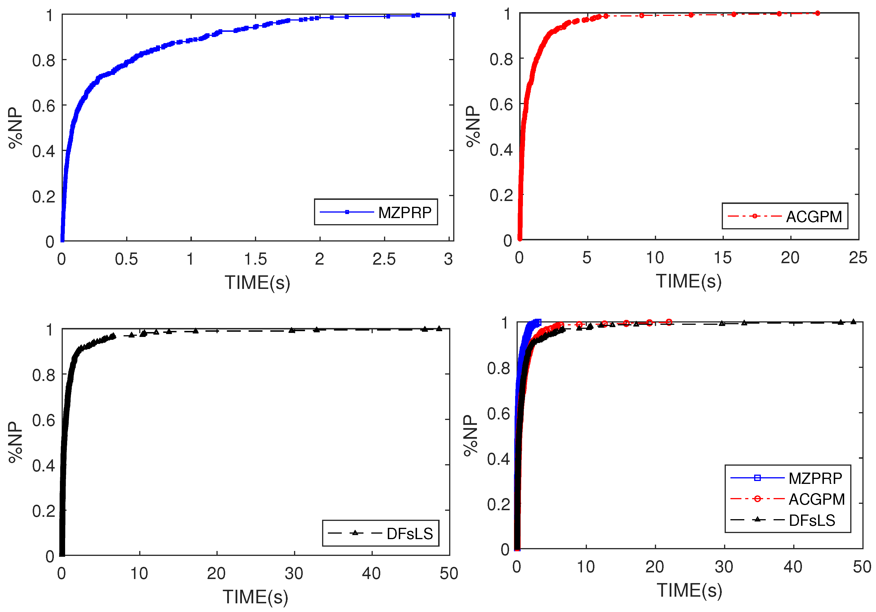
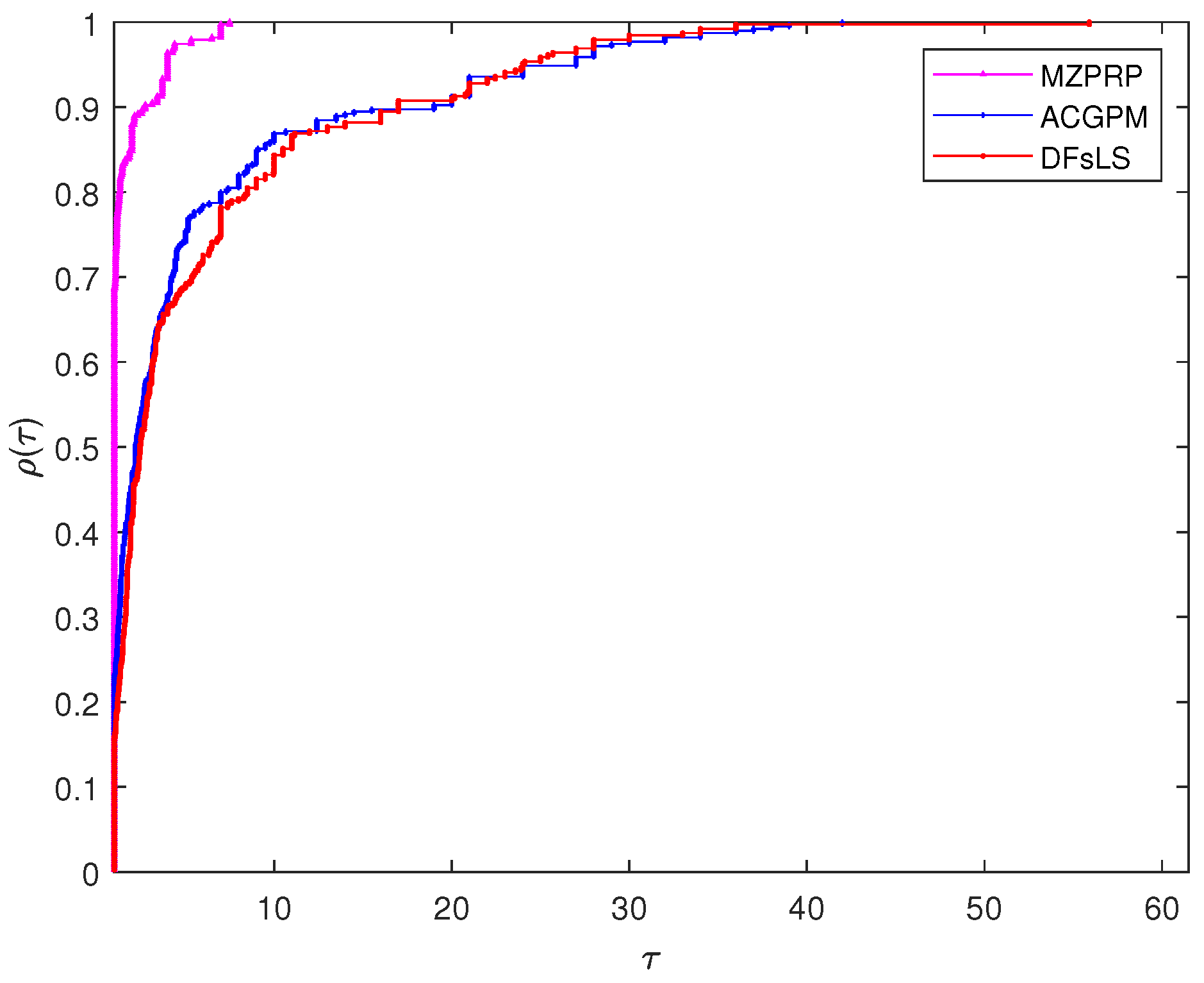
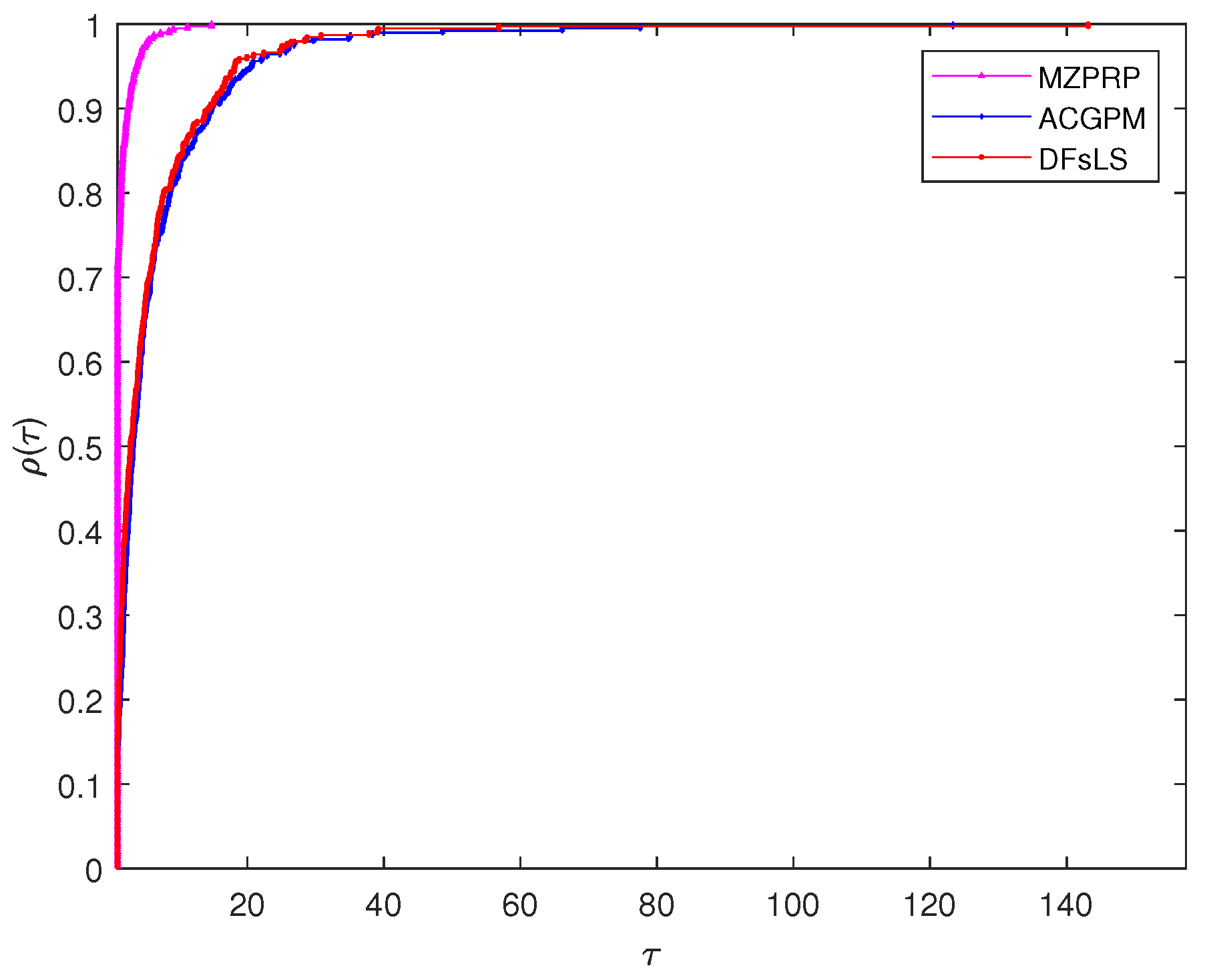
4. Numerical Experiments

In this section, we present numerical experiments to assess the numerical performance of the proposed MZPRP in comparison with the following two existing methods, namely:

(i)

“A conjugate gradient projection method for solving equations with convex constraints” proposed by Zheng et al. [38]. For convenience, we denote this method as ACGPM.

(ii)

“Partially symmetrical derivative-free Liu–Storey projection method for convex constrained equations” developed by Liu et al. [39]. For simplicity, this method shall be denoted by DFsLS.

In this experiment, we consider thirteen (13) test problems (see, Appendix A) where each problem is solved using six starting points (SP) by varying the dimensions as 1000, 5000, 10,000, 50,000, 100,000. The SPs used for each problem are given as follows: $x_1={(\frac{1}{10},\frac{1}{10},\frac{1}{10},\dots ,\frac{1}{10})}^T,$$x_2={(\frac{1}{2},\frac{1}{2^2},\frac{1}{2^3},\dots ,\frac{1}{2^n})}^T,$$x_3={(2,2,2,\dots ,2)}^T,$$x_4={(1,\frac{1}{2},\frac{1}{3},\dots ,\frac{1}{n})}^T,$$x_5={(1-\frac{1}{n},1-\frac{2}{n},1-\frac{3}{n},\dots ,0)}^T$ and $x_6=\mathrm{rand}(0,1).$ This means that the number of problems solved by each method in the course of this experiment is three hundred and ninety (390). The three methods, that is MZPRP, ACGPM and DFsLS were coded in MATLAB R2019b which was on a PC with the following specifications: Intel Core(TM) i5-8250u processor with 4 GB of RAM and CPU 1.60 GHZ. In the course of execution, we used the following parameters for MZPRP $h=5,$$\rho =0.5,$$\alpha =0.1,$$c=0.01,$$\sigma =0.01,\kappa =1,$ and $\ell =1.99.$ The parameters used for ACGPM and DFsLS are as presented in [38,39]. During the iteration process, a method is declared to have achieved an approximate solution whenever $\parallel \mathsf{\Omega }\left(x_k\right)\parallel \le {10}^{-6}.$ On the other hand, if the number of iterations surpasses 1000 iterations and the stopping criterion mentioned above has not been satisfied, then a failure is declared. To visualise the performance of each algorithm, we employ the following metrics: ITER (number of iterations), FVAL (number of function evaluations) and TIME (CPU time). Moreover, as the iteration process terminates, we report $\parallel \mathsf{\Omega }\left(x^{*}\right)\parallel$ (denoted by NORM) to ascertain whether a method successfully obtained a solution of a particular problem or not. The detailed report of the numerical results of the proposed MZPRP method, the ACGPM method [38] and the DFsLS method [39] are tabulated and can be found in the link https://github.com/aliyumagsu/MZPRP_Exp_Tables (accessed on 24 July 2022). The numerical data are summarised using a data profile (see Figure 1, Figure 2 and Figure 3) which shows the required ITER, FVAL, as well as the TIME budget for each of the three methods to successfully solve the test problems considered in this experiment. The data profile plots %NP (percentage of the number of problem) versus ITER in Figure 1, %NP versus FVAL in Figure 2 and %NP versus TIME in Figure 3. In essence, Figure 1 gives the required ITER budget for a method to solve a certain percentage of the 390 test problems considered for this experiment. This means, considering Figure 1 (top-left, top-right and bottom left), we see that with a budget of 30 ITER, the new method (MZPRP) successfully solves more than 95% of the problems, while ACGPM and DFsLS will only solve 65% and 70% of the problems, respectively. Similarly, if we consider Figure 3 (top-left, top-right and bottom left), we see that, with a budget of 1.5 s, the MZPRP will solve 95% of the test problems, as against ACGPM and DFsLS, that will solve about 80% of the same test problems. This suggests that the new MZPRP is computationally cheaper compared to the existing ACGPM and DFsLS.

In addition, we use the performance profile proposed by Dolan and Moré in [40] to obtain Figure 4, Figure 5 and Figure 6, which is a standard tool for comparing iterative methods. Figure 4 shows the number of iterations for the performance profile of the MZPRP, the ACPGM, and the DFsLS methods. Figure 5 presents the performance profile based on the number of function evaluations; the CPU time performance profile is reported in Figure 6. From Figure 4, Figure 5 and Figure 6, we can see that the proposed MZPRP method produces better results than ACPGM and DFsLS with a higher percentage in ITER, FVAL and TIME.

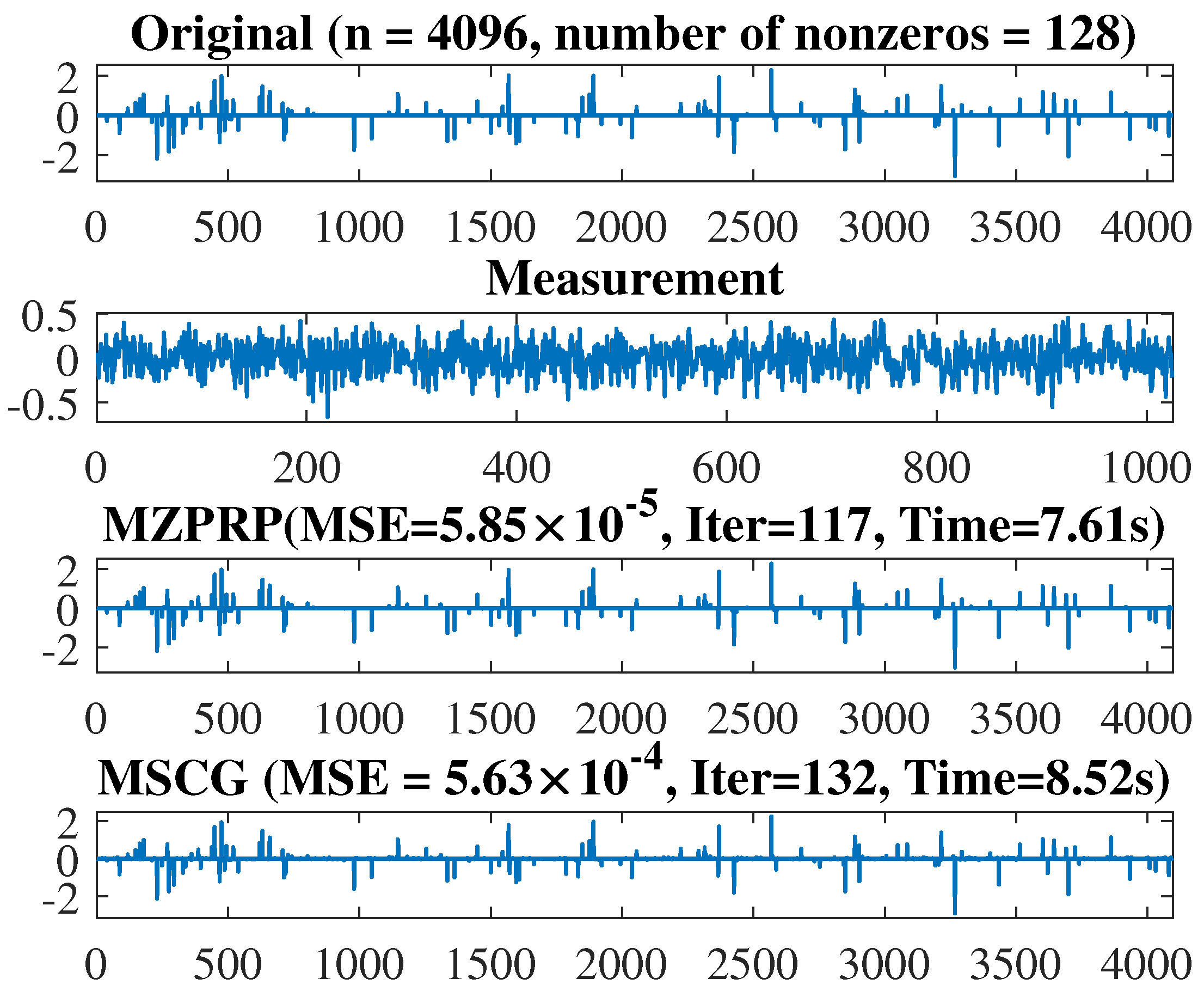
5. Application in Compressive Sensing

Applications of derivative-free algorithms in compressive sensing have recently received more attention. As described in [41], signal processing involves solving the following problem

$$\underset{x}{min}\omega \left(x\right),\omega \left(x\right)=\frac{1}{2}{\parallel y-Qx\parallel }_2^2+\eta {\parallel x\parallel }_1,$$

(35)

containing a quadratic error term and a sparse ${\ell }_1$-regularization term where $\eta >0$ is a regularization parameter, $x\in {\mathbb{R}}^n$, $y\in {\mathbb{R}}^k$ is an observation, and $Q\in {\mathbb{R}}^{k\times n}$ ($k<<n$) is a linear operator. It is clear that (35) is a non-smooth problem. To smooth it, Figueiredo et al. [41] split the vector x into two as $x=a-b$ with $a_i={\left(x_i\right)}_{+}$ and $b_i={(-x_i)}_{+}$ where ${(·)}_{+}=max\{0,·\}$ and $i=1,2,\dots ,n.$ This resulted in the following smooth problem

$$\underset{q\ge 0}{min}\frac{1}{2}{q}^{T}Zq+r^{T}q,$$

(36)

where $q={\left[ab\right]}^T,$ $r=\eta e_{2n}+{\left[-Q^{T}y{Q}^{T}y\right]}^T$ and $Z=\left[\begin{array}{cc}{Q}^{T}Q& -Q^{T}Q\\ -Q^{T}Q& Q^{T}Q\end{array}\right]$. It is also clear that (36) is a convex quadratic problem, since the square matrix Z is a positive semi-definite.

Inspired by the transformation of Figueiredo et al. [41], Xiao et al. [42] decided to further reformulate (36) into the following system of nonlinear equations

$$\mathsf{\Omega }\left(q\right)=min\{q,Zq+r\}=0,$$

(37)

where the “min” is interpreted as a component-wise minimum. The major advantage of the reformulation (37) is that it can be solved without the necessary knowledge of the gradient of $\omega \left(x\right)$ in (35). This means a derivative-free algorithm, such as Algorithm 1 (MZPRP), can be employed to solve it successfully.

However, two major assumptions, namely pseudomonotonicity and Lipschitz continuity, were used in establishing the convergence result of Algorithm 1 (MZPRP). Interestingly, Pang [43] has shown that the mapping $\mathsf{\Omega }$ in (37) is Lipschitz continuous and, on the other hand, Xiao et al. [42] proved that it is also monotone. Since every monotone function is pseudomonotone, our convergence results still stand.

In what follows, we give the description of the signal recovery experiment. We consider the reconstruction of a sparse signal of size $n=2^{11}$ from $k=2^9$ observations. The original signal contains $2^7$ randomly non-zero elements with the measurement vector v being distributed with some noise, $v=Q\tilde{x}+\overline{\varrho },$ where Q is a randomly generated Gaussian matrix and $\overline{\varrho }$ is the Gaussian noise distributed normally with mean 0 and variance ${10}^{-4}.$ The signal recovery experiment was performed using MATLAB R2019b installed on a PC with an Intel Core(TM) i5-8250u processor with 4 GB of RAM and CPU 1.60 GHZ.

For this experiment, we compare the new Algorithm 1 (MZPRP) with the existing algorithm (MSCG) developed in [44] based on: (i) the number of iterations; (ii) CPU time taken to successfully recover the disturb signal; and (iii) the means of square error (MSE) used to measure the quality of the reconstruction of the disturbed signal with respect to the original signal $\tilde{x}$; that is, $MSE=\frac{1}{n}{\parallel \tilde{x}-x_{*}\parallel }^2,$ where $x_{*}$ is the recovered signal. We successfully implemented the MZPRP using the same parameters given in the preceding section, while the parameters used for MSCG are as presented in [44]. We run the two algorithms from the same initial point $x_0=Q^{T}y$ and the same continuation technique on the parameter $\eta$. We set the termination criteria as

$$\left|\frac{\omega \left(x_k\right)-\omega \left(x_{k-1}\right)}{\omega \left(x_{k-1}\right)}\right|<{10}^{-5},$$

throughout the experiment.

The numerical performance of each algorithm is assessed by Iter (number of iterations) and Time (CPU time) required to successfully recover the disturbed signal. In addition, the quality of the reconstruction of the disturbed signal is assessed by MSE (mean of squared error) to the original signal $\tilde{x}.$ The formula for the MSE is given as $MSE=\frac{1}{n}{\parallel \tilde{x}-x_{*}\parallel }^2,$ where $x_{*}$ is the recovered signal.

We report the numerical results in Figure 7 and Figure 8 where Figure 7 reveals that both the MZPRP and MSCG algorithms recovered the disturbed signal successfully. Though it is difficult to visualize the algorithm with a better quality, the MSE recorded by the two algorithms suggests that the quality of recovery by MZPRP is better than that of MSCG. Based on the CPU time recorded by both algorithms, it can be seen that MZPRP recovers the disturbed signal faster that MSCG. These observations, coupled with the number of iterations, show that the MZPRP is more efficient than MSCG and hence underscores the applicability of the new method.

6. Conclusions

In this paper, we proposed a derivative-free method for large-scale nonlinear systems of equations where the underlying function is assumed to be pseudomonotone. It is worth noting that pseudomonotonicity is a weaker assumption than monotonicity. The global convergence of the proposed method has been discussed based on the assumption that the problem under consideration satisfies Lipschitz continuity. Numerical comparison with that of ACGPM [38] and DFsLS [39] derivative-free methods demonstrated the efficiency of the new method, as well as its superior numerical performance. As an application, the new method has been successfully implemented to solve a signal recovery problem arising from compressive sensing. Future work will concentrate on applying the new method to solve 2D robotic motion control.

References

1. Fang, X. Class of new derivative-free gradient type methods for large-scale nonlinear systems of monotone equations. J. Inequalities Appl. 2020, 2020, 93. [Google Scholar] [CrossRef]
2. Schnabel, R.B.; Dennis, J.E., Jr. Numerical Methods for Unconstrained Optimization and Nonlinear Equations; Prentice-Hall: Englewood Cliffs, NJ, USA, 1983. [Google Scholar]
3. Grippo, L.; Lampariello, F.; Lucidi, S. A Nonmonotone Line Search Technique for Newton’s Method. SIAM J. Numer. Anal. 1986, 23, 707–716. [Google Scholar] [CrossRef]
4. Morini, B.; Bellavia, S. A globally convergent Newton-GMRES subspace method for systems of nonlinear equations. SIAM J. Sci. Comput. 2001, 23, 940–960. [Google Scholar]
5. Martínez, J.M.; Birgin, E.G.; Krejic, N.K. Globally convergent inexact quasi-Newton methods for solving nonliear systems. Numer. Algorithms 2003, 32, 249–260. [Google Scholar]
6. Gasparo, M.G. A nonmonotone hybrid method for nonlinear systems. Optim. Method Softw. 2000, 13, 79–94. [Google Scholar] [CrossRef]
7. Broyden, C.G. A class of methods for solving nonlinear simultaneous equations. Math. Comput. 1965, 19, 577–593. [Google Scholar] [CrossRef]
8. Nesterov, Y.; Rodomanov, A. New results on superlinear convergence of classical quasi-Newton methods. J. Optim. Theory Appl. 2021, 188, 744–769. [Google Scholar]
9. Rodomanov, A.; Nesterov, Y. Greedy quasi-Newton methods with explicit superlinear convergence. SIAM J. Optim. 2021, 31, 785–811. [Google Scholar] [CrossRef]
10. Borwein, J.M.; Barzilai, J. Two-point step size gradient methods. IMA J. Numer. Anal. 1988, 8, 141–148. [Google Scholar]
11. Raydann, M.; Cruz, W.L.; Martinez, J.M. Spectral residual method without gradient information for solving large-scale nonlinear systems of equations. Math. Comput. 2006, 75, 1429–1448. [Google Scholar]
12. Solodov, M.V.; Svaiter, B.F. A globally convergent inexact Newton method for systems of monotone equations. In Reformulation: Nonsmooth, Piecewise Smooth, Semismooth and Smoothing Methods; Springer: Boston, MA, USA, 1998; pp. 355–369. [Google Scholar]
13. Yu, Z.; Lin, J.; Sun, J.; Xiao, Y.; Liu, L.; Li, Z. Spectral gradient projection method for monotone nonlinear equations with convex constraints. Appl. Numer. Math. 2009, 59, 2416–2423. [Google Scholar] [CrossRef]
14. Zhang, L.; Zhou, W. Spectral gradient projection method for solving nonlinear monotone equations. J. Comput. Appl. Math. 2006, 196, 478–484. [Google Scholar] [CrossRef]
15. Muhammed, A.A.; Kumam, P.; Abubakar, A.B.; Wakili, A.; Pakkaranang, N. A new hybrid spectral gradient projection method for monotone system of nonlinear equations with convex constraints. Thai J. Math. 2018, 125–147. [Google Scholar]
16. Awwal, A.M.; Wang, L.; Kumam, P.; Mohammad, H. A two-step spectral gradient projection method for system of nonlinear monotone equations and image deblurring problems. Symmetry 2020, 12, 874. [Google Scholar] [CrossRef]
17. Sulaiman, I.M.; Mamat, M. A new conjugate gradient method with descent properties and its application to regression analysis. J. Numer. Anal. Ind. Appl. Math. 2020, 14, 25–39. [Google Scholar]
18. Malik, M.; Mamat, M.; Abas, S.S.; Sulaiman, I.M.; Sukono, F. A new coefficient of the conjugate gradient method with the sufficient descent condition and global convergence properties. Eng. Lett. 2020, 28, 704–714. [Google Scholar]
19. Yakubu, U.A.; Sulaiman, I.M.; Mamat, M.; Ghazali, P.L.; Khalid, K. The global convergence properties of a descent conjugate gradient method. J. Adv. Res. Dyn. Control Syst. 2020, 12, 1011–1016. [Google Scholar]
20. Stiefel, E.; Hestenes, M.R. Methods of conjugate gradients for solving linear systems. J. Res. Natl. Bur. Stand. 1952, 49, 409–436. [Google Scholar]
21. Fletcher, R.; Reeves, C.M. Function minimization by conjugate gradients. Comput. J. 1964, 7, 149–154. [Google Scholar] [CrossRef]
22. Ribiere, G.; Polak, E. Note sur la convergence de méthodes de directions conjuguées. ESAIM Math. Model. Numer. Anal.-Modél. Math. Anal. Numér. 1969, 3, 35–43. [Google Scholar]
23. Malik, M.; Mamat, M.; Abas, S.S.; Sulaiman, I.M.; Sukono, F. A new modification of NPRP conjugate gradient method for unconstrained optimization. Adv. Math. Sci. J. 2020, 9, 4955–4970. [Google Scholar] [CrossRef]
24. Storey, C.; Liu, Y. Efficient generalized conjugate gradient algorithms, part 1: Theory. J. Optim. Theory Appl. 1991, 69, 129–137. [Google Scholar]
25. Fletcher, R. Practical Methods of Optimization; John Wiley & Sons: Hoboken, NJ, USA, 2013. [Google Scholar]
26. Yuan, Y.; Dai, Y.H. A nonlinear conjugate gradient method with a strong global convergence property. SIAM J. Optim. 1999, 10, 177–182. [Google Scholar]
27. Rivaie, M.; Mamat, M.; Abashar, A. A new class of nonlinear conjugate gradient coefficients with exact and inexact line searches. Appl. Math. Comput. 2015, 268, 1152–1163. [Google Scholar] [CrossRef]
28. Awwal, A.M.; Kumam, P.; Abubakar, A.B. Spectral modified Polak–Ribiére–Polyak projection conjugate gradient method for solving monotone systems of nonlinear equations. Appl. Math. Comput. 2019, 362, 124514. [Google Scholar] [CrossRef]
29. Awwal, A.M.; Wang, L.; Kumam, P.; Mohammad, H.; Watthayu, W. A projection Hestenes-Stiefel method with spectral parameter for nonlinear monotone equations and signal processing. Math. Comput. Appl. 2020, 2, 27. [Google Scholar] [CrossRef]
30. Awwal, A.M.; Kumam, P.; Wang, L.; Huang, S.; Kumam, W. Inertial-based derivative-free method for system of monotone nonlinear equations and application. IEEE Access 2020, 8, 226921–226930. [Google Scholar] [CrossRef]
31. Cheng, W.; Xiao, Y.; Hu, Q.J. A family of derivative-free conjugate gradient methods for large-scale nonlinear systems of equations. J. Comput. Appl. Math. 2009, 224, 11–19. [Google Scholar] [CrossRef]
32. Zhu, H.; Xiao, Y. A conjugate gradient method to solve convex constrained monotone equations with applications in compressive sensing. J. Math. Anal. Appl. 2013, 405, 310–319. [Google Scholar]
33. Zhang, H.; Hager, W. A new conjugate gradient method with guaranteed descent and an efficient line search. SIAM J. Optim. 2005, 16, 170–192. [Google Scholar]
34. Min, L. A derivative-free PRP method for solving large-scale nonlinear systems of equations and its global convergence. Optim. Methods Softw. 2014, 29, 503–514. [Google Scholar]
35. Qin, N.; Xiaowei, F. A new derivative-free conjugate gradient method for large-scale nonlinear systems of equations. Bull. Aust. Math. Soc. 2017, 95, 500–511. [Google Scholar]
36. Sabi’u, J.; Waziri, M.Y. A derivative-free conjugate gradient method and its global convergence for solving symmetric nonlinear equations. Int. J. Math. Math. Sci. 2015, 2015, 961487. [Google Scholar]
37. Zheng, X.; Shi, J. A modified sufficient descent Polak–Ribiére–Polyak type conjugate gradient method for unconstrained optimization problems. Algorithms 2018, 11, 133. [Google Scholar] [CrossRef]
38. Zheng, L.; Yang, L.; Liang, Y. A conjugate gradient projection method for solving equations with convex constraints. J. Comput. Appl. Math. 2020, 375, 112781. [Google Scholar] [CrossRef]
39. Liu, J.K.; Xu, J.Ł.; Zhang, L.Q. Partially symmetrical derivative-free Liu–Storey projection method for convex constrained equations. Int. J. Comput. Math. 2019, 96, 1787–1798. [Google Scholar] [CrossRef]
40. Dolan, E.D.; Moré, J.J. Benchmarking optimization software with performance profiles. Math. Program. 2002, 91, 201–213. [Google Scholar] [CrossRef]
41. Figueiredo, M.A.T.; Nowak, R.D.; Wright, S.J. Gradient projection for sparse reconstruction: Application to compressed sensing and other inverse problems. IEEE J. Sel. Top. Signal Process. 2007, 1, 586–597. [Google Scholar] [CrossRef]
42. Xiao, Y.; Wang, Q.; Hu, Q. Non-smooth equations based method for 1-norm problems with applications to compressed sensing. Nonlinear Anal. Theory Methods Appl. 2011, 74, 3570–3577. [Google Scholar] [CrossRef]
43. Pang, J.S. Inexact Newton methods for the nonlinear complementarity problem. Math. Program. 1986, 36, 54–71. [Google Scholar] [CrossRef]
44. Abubakar, A.B.; Kumam, P.; Awwal, A.M.; Thounthong, P. A modified self-adaptive conjugate gradient method for solving convex constrained monotone nonlinear equations for signal recovery problems. Mathematics 2019, 7, 693. [Google Scholar] [CrossRef]
45. Awwal, A.M.; Kumam, P.; Abubakar, A.B. A modified conjugate gradient method for monotone nonlinear equations with convex constraints. Appl. Numer. Math. 2019, 145, 507–520. [Google Scholar] [CrossRef]
46. Aji, S.; Kumam, P.; Awwal, A.M.; Yahaya, M.M.; Sitthithakerngkiet, K. An efficient DY-type spectral conjugate gradient method for system of nonlinear monotone equations with application in signal recovery. AIMS Math. 2021, 6, 8078–8106. [Google Scholar] [CrossRef]
47. Awwal, A.M.; Kumam, P.; Sitthithakerngkiet, K.; Bakoji, A.M.; Halilu, A.S.; Sulaiman, I.M. Derivative-free method based on DFP updating formula for solving convex constrained nonlinear monotone equations and application. AIMS Math. 2021, 6, 8792–8814. [Google Scholar] [CrossRef]
Figure 1. Data Profile: %NP versus ITER.
Mathematics 10 02884 g001
Figure 2. Data Profile: %NP versus FVAL.
Mathematics 10 02884 g002
Figure 3. Data Profile: %NP versus TIME(s).
Mathematics 10 02884 g003
Figure 4. Performance profiles for MZPRP, ACGPM and DFsLS based on ITER.
Mathematics 10 02884 g004
Figure 5. Performance profiles for MZPRP, ACGPM and DFsLS based on FVAL.
Mathematics 10 02884 g005
Figure 6. Performance profiles for MZPRP, ACGPM and DFsLS based on TIME.
Mathematics 10 02884 g006
Figure 7. From top to bottom: The original signal, the measurement, the recovered signal by the MZPRP and MSCG methods, respectively.
Mathematics 10 02884 g007
Figure 8. Comparison result of the MZPRP and MSCG methods. The x-axis represents the number of iterations (top left and bottom left), and the CPU time in seconds (top right and bottom right). The y-axis represents the MSE (top left and top right) and the objective function values (bottom left and bottom right).
Mathematics 10 02884 g008
Publisher’s Note: MDPI stays neutral with regard to jurisdictional claims in published maps and institutional affiliations.