
Sawi Transform Based Homotopy Perturbation Method for Solving Shallow Water Wave Equations in Fuzzy Environment


Department of Mathematics, National Institute of Technology Rourkela, Rourkela 769008, India
*
Author to whom correspondence should be addressed.
Mathematics 2022, 10(16), 2900; https://0-doi-org.brum.beds.ac.uk/10.3390/math10162900
Submission received: 14 July 2022
/
Revised: 9 August 2022
/
Accepted: 10 August 2022
/
Published: 12 August 2022
(This article belongs to the Special Issue Computational Methods in Nonlinear Analysis and Their Applications)
Abstract
:In this manuscript, a new hybrid technique viz Sawi transform-based homotopy perturbation method is implemented to solve one-dimensional shallow water wave equations. In general, the quantities involved with such equations are commonly assumed to be crisp, but the parameters involved in the actual scenario may be imprecise/uncertain. Therefore, fuzzy uncertainty is introduced as an initial condition. The main focus of this study is to find the approximate solution of one-dimensional shallow water wave equations with crisp, as well as fuzzy, uncertain initial conditions. First, by taking the initial condition as crisp, the approximate series solutions are obtained. Then these solutions are compared graphically with existing solutions, showing the reliability of the present method. Further, by considering uncertain initial conditions in terms of Gaussian fuzzy number, the governing equation leads to fuzzy shallow water wave equations. Finally, the solutions obtained by the proposed method are presented in the form of Gaussian fuzzy number plots.
Keywords:
Gaussian fuzzy numbers; shallow water wave equations; fuzzy shallow water wave equations; Sawi transform-based homotopy perturbation methodMSC:
03E72; 76B15; 35Q351. Introduction
The shallow water wave equations (SWWEs) are used extensively to simulate the spread of tsunami waves, storm floods, tidal currents, shock waves, etc. These waves occur near the shore as the waves approach the coastal zone. Due to the high importance of the SWWEs in engineering and science, different numerical methods, as well as analytical and semi-analytical methods, were suggested in the past to replicate the SWWEs, such as the finite element method (FEM), variational iteration method (VIM), finite volume method (FVM), finite difference method (FDM), Adomian decomposition method (ADM), the homotopy perturbation method (HPM), etc. In this regard, Safari [1] used the ADM to solve two extended model equations for shallow water waves (SWWs) in an analytic manner. Benkhaldoun and Seaidb [2] provided a new FVM to find the numerical solution for SWWEs over flat or non-flat topography using a predictor corrector strategy. Busto and Dumbser [3] discussed a novel staggered semi-implicit hybrid FVM/FEM for solving SWWEs on unstructured meshes at all Froude numbers. Carfora [4] examined the use of a grid point numerical approach to solve atmospherical shallow water problems. Wu et al. [5] used an explicit predictor corrector approach to develop a numerical model for finding solutions to SWWEs. Tsunamis are instances of such waves, and tsunami models frequently use shallow water equations. As such, Cho et al. [6] suggested a numerical scheme based on linear SWWEs for modeling the distance propagation of tsunamis. Liu et al. [7] investigated the use of linear and nonlinear equations of SWWs in tsunami predictions.
Additionally, SWWEs are a set of hyperbolic partial differential equations, and many real-world events are governed by integer-order partial differential equations that are difficult to explain. Consequently, fractional-order nonlinear partial differential equations are of equal importance. In this regard, the fractional reduced differential transform method (FRDTM) was used to analyze the mathematical model of tsunami wave propagation along a coastline of an ocean in [8]. A study by Patel et al. [9] uses the FRDTM to analyze the behavior of fractional-order shallow fluid equations and investigate applications to a model of time fractional-order atmospheric waves propagating in a fluid medium. They also applied FRDTM to obtain the approximate solutions of the time-fractional diffusion equation and Cahn–Allen equation arising in oil pollution [10]. In addition, Patel and Patel [11] successfully applied this method to obtain analytical approximate solutions to the nonlinear generalized fractional-order Fitzhugh–Nagumo equation. The approximate solution was also obtained in [12] for the time-fractional (2 + 1) dimensional Wu–Zhang nonlinear system, which describes a long dispersive wave.
SWWEs and FSWWEs were solved using an efficient method (VIM) by He [13]. Linear, nonlinear, and coupled differential equations can be solved with VIM. Various researchers carried out interesting research on this strategy. Wazwaz [14] used VIM to solve both linear and nonlinear wave equations and a system of partial differential equations analytically. Additionally, Wazwaz [15] carried out an excellent study using VIM to solve both linear and nonlinear Schrodinger equations. Kang-Le Wang [16] used fractal calculus to study the shallow water wave with unsmooth borders, and He used VIM to find the exact solution of a fractal solitary wave.
Mansfield and Clarkson [17] derived some symmetries and accurate solutions to the (2 + 1) dimensional SWWE. Bernetti et al. [18] solved the Riemann problem for nonlinear equations of SWWs with discontinuous bottom shapes using a second-order upwind TVD method. Wazwaz [19,20] provided multiple-soliton solutions for two and three extension models of shallow water wave model equations. For SWWEs, LeFloch and Thanh [21] introduced numerical experiments that show the convergence of the Godunov-type scheme based on the Riemann solver, and they also inspect the Riemann problem for equations of SWWs with variable and discontinuous topography. Bekir and Aksoy [22] used the exp-function approach to determine the exact solution to the extended SWWEs in two and three dimensions. Using the Hirota bilinear approach and the long-wave limit method, Jiayue, Yong, and Huanhe [23] examined the (3 + 1) dimensional SWWE and discovered the rational solutions and interaction solutions based on N-soliton solutions. The conventional truncated Painlevé analysis was used by Xin et al. [24] to determine the Schwartzian equation of the (2 + 1) dimensional generalized variable coefficient SWWEs. They also employed the closed system’s Lie point symmetries and the Schwartzian equation to find some precise interaction solutions, such as soliton–cnoidal wave solutions. Wang [25] used the fractal semi-inverse method to establish the fractal Boussinesq-like equation and also proposed the variational transform method to find the exact fractal solitary wave solution for the fractal nonlinear dispersive Boussinesq-like equation.
Clements and Rogers [26] conducted a successful and valuable effort to get analytical solutions to the linearized SWWEs. The sine-Gordon expansion method was used by Mehmet and Yuzuncu [27] to extract some complex soliton solutions to the (2 + 1) dimensional extended SWW model, which explains the evolution of SWW propagation. Noeiaghdam et al. [28] applied the semi-analytical homotopy analysis method (HAM) to solve the nonlinear SWWE. They authenticated their numerical results by using stochastic arithmetic, the CESTAC procedure, and the CADNA library. A new (2 + 1) dimensional extended SWWE was investigated analytically by Adeyemo and Khaliqu [29] to arrive at a series solution to the equation. The shallow water model can be seen as essentially a convection–diffusion–reaction model [30]. In this regard, Salnikov and Siryk [31,32,33] proposed the Petrov–Galerkin method, as well as the modification of the Petrov−Galerkin method, for constructing continuous piecewise polynomial weight functions in two and three-dimensional domains. A finite number of variable parameters associated with the edges of a grid partition determine the form of such functions. John et al. [34] describe important results regarding FEM for convection-dominated problems and incompressible flow problems. They also concentrated on H1-conforming FEM, with a few exceptions for incompressible flow problems.
Among all of the methods mentioned above, the HPM, which was first introduced by He [35], plays a significant role. This is because it directly handles an issue without requiring any kind of transformation, linearization, or discrimination. Chen and An [36] used HPM to solve nonlinear coupled equations with parameter derivatives, while Hemeda [37] used HPM to solve nonlinear coupled equations viz. the systems of coupled Burgers’ equations in one and two dimensions. Additionally, HPM was employed by Sheikholeslami et al. [38] to investigate micropolar fluid flow in a channel undergoing a chemical reaction. Kumar et al. [39] compared the modified homotopy analysis transform method to the residual power series method for solving time-fractional coupled SWWEs. Singh et al. [40] proposed a new modification of the HPM to solve nonlinear and singular time-dependent Emden–Fowler-type equations with Neumann and Dirichlet boundary conditions. Karunakar and Chakraverty [41] used HPM to solve coupled one-dimensional linear and nonlinear SWWEs with Gaussian-type initial conditions, yielding interesting results that are graphically compared. Recently, using HPM, Dubey and Chakraverty [42] solved both one-dimensional and two-dimensional fractional wave equations with boundary conditions. Karunakar and Chakraverty [43] employed the homotopy perturbation transform method to solve interval differential equations, resulting in the solution of the interval-modified Kawahara differential equation, which represents nonlinear water waves in the long wavelength regime. Sawi transform (ST) is a new integral transform that was proposed by Mohand Mahgoub in 2019 [44]. ST is well known for its ability to solve linear ordinary and partial differential equations as well as integral equations. As the SWWEs form a system of hyperbolic partial differential equations, it may be interesting to solve using the combination of ST and HPM (i.e., SHPM).
It may be observed that complete information regarding the parameter involved in the governing equation of SWWEs is not always available. As a result, fuzzy parameters could be included in the governing equation of SWWEs. In this regard, the behavior of two-dimensional SWWEs with fuzzy parameters was investigated by Karunakar and Chakraverty [45]. They used HPM to solve the SWWEs by treating the water depth as uncertain in terms of fuzzy. Additionally, Chakraverty and Karunakar [46] suggested a strategy for dealing with crisp and uncertain differential equations that regulate shallow water equations. They did this by using HPM to solve nonlinear SWWE in a crisp and precise context, specifically for tsunami wave propagation.
In view of the preceding literature review, we noticed that there was not much research on solving SWWEs with fuzzy parameters. Therefore, in this research, we proposed a novel method SHPM, i.e., HPM along with a new transform called Sawi transform (ST), and solved SWWEs in crisp, as well as fuzzy environments by taking the initial condition as the Gaussian fuzzy number. For the crisp case, we gave a comparison study with [41].
The remainder of the paper is structured as follows. In Section 2, we cover some essential fuzzy concepts and notations and also discuss the governing differential equations of SWWEs. In Section 3, a brief overview of the Sawi transform (ST) along with some of its properties are presented. Section 4 describes the proposed method, i.e., SHPM to find the solution of linear SWWEs in crisp as well as fuzzy environments. In Section 5, we provide numerical results from the suggested technique in both crisp and fuzzy cases and the effectiveness of the proposed method is displayed graphically by comparing the solutions of linear SWWEs obtained by SHPM and HPM. Finally, in Section 6, the results from the present investigation are summarized, and future directions are suggested.
2. Preliminaries
The essential fuzzy concepts and notations that will be used throughout this study and the governing SWWEs are discussed in this section.
2.1. Fuzzy Set [47]
A fuzzy set may be defined as a collection of a set of order pairs, i.e.,
where, is known as the membership function of and be the universal set.
2.2. Fuzzy Number [47]
A fuzzy number is a particular type of fuzzy set , which is normalized and convex having a piecewise continuous membership function.
2.3. of a Fuzzy Number [47]
For a fuzzy set in and any real number , the of , denoted by is the crisp set and may be interpreted as
2.4. Gaussian Fuzzy Number (GFN) [47,48]
A Gaussian fuzzy number (where and represent the mean and the standard deviation, respectively), as given in Figure 1, is a bell-shaped fuzzy number having a membership function for , where
Note. If and are the same (i.e., ) for a Gaussian fuzzy number , then it is said to be a symmetric Gaussian fuzzy number (SGFN) and is defined by . The membership function of such a fuzzy number can be written as
2.5. Representation of SGFN [47,48]
In the case of SGFN , the fuzzy interval form using is obtained as
2.6. Double Parametric Form of SGFN [47,48]
Implementing another parameter on Equation (5), we may have the following expression
where and .
The above Equation (6) is named as double parametric form, as it involves two parameters viz. and .
2.7. Shallow Water Wave Equations (SWWEs) [6]
The coupled linear one-dimensional SWWEs may be written as follows
where,
- is the water surface elevation (WSE),
- is the time,
- is the depth-averaged volume flux in the direction,
- is the acceleration due to gravity , and
- is the water depth.
3. Sawi Transform (ST) and Some of Its Properties
The ST, its properties, and ST of some functions are briefly discussed in this section.
3.1. Sawi Transform (ST) [44]
Sawi transform was proposed by Mahgoub, in 2019 [44]. ST of the function belongs to a class , where
For a given function in the set is a constant finite number and may be finite or infinite. ST is denoted by the operator and may be defined by the integral equation:
The variable in this transform is used to factor the variable t in the argument of the function . If is piecewise continuous and of exponential order, the ST of the function , exist otherwise ST may or may not exist.
3.2. Linearity Property of ST [44]
If and , then where and are arbitrary constants.
3.3. ST of Some Useful Functions [44]
ST of some useful functions is listed in Table 1.
3.4. Inverse ST of Some Useful Functions [44]
If , then can be treated as the inverse ST of . Mathematically it is defined as , where is called the inverse ST operator. The explicit form of inverse ST can be written as the following formula:
Inverse ST of some useful functions are listed in Table 2.
3.5. Sawi Transform of Partial Derivatives [49]
Let . To obtain ST of a partial derivative we use integration by parts, and then we have
- 1.
- 2.
- 3.
- 4.
Using mathematical induction, we can simply extend this result to the partial derivative.
4. Homotopy Perturbation Method (HPM) [35]
The basic concept of HPM is demonstrated in this section.
Let us consider the following differential equation:
Subject to the boundary conditions
where denotes a general differential operator, is a boundary operator, is the boundary of the domain , and is known as an analytic function.
The operator can be separated into two parts: linear () and nonlinear (). As a result, Equation (11) may be expressed as follows:
In Equation (13) an artificial parameter can be inserted as follows:
Now using the homotopy technique, let us construct a homotopy , that satisfies
or
where is an initial approximation of Equation (11) that fulfills the boundary constraints, and is an embedding parameter. We may deduce the following from Equations (15) or (16):
changes from to as rises from zero to unity. This is regarded as deformation in topology, where and are referred to as homotopic. As is a small parameter, we treat the solution of Equation (13) as a power series in as follows:
Setting yields the following approximate solution to Equation (11):
5. Methodology
In the upcoming subsections, the proposed method, i.e., SHPM is briefly discussed to solve the governing linear equations of SWWs. This is being employed to one-dimensional SWWs with crisp, as well as fuzzy, initial conditions that are in Gaussian form. This is accomplished by using MATLAB software ‘9.9.0.1524771 (R2020b) (MATLAB, NIT Rourkela, India).
5.1. An Algorithm for Sawi Transform Based Homotopy Perturbation Method (SHPM)
In this section, an Algorithm 1 is discussed for solving the governing differential eqution by using the proposed technique.
| Algorithm1. An Algorithm for Solving a Differential Equation by Using SHPM | |
| Step 1: | Write down the governing differential equation |
| Step 2: | Apply Sawi transform in the governing differential equation |
| Step 3: | Use differential and integral properties of ST |
| Step 4: | Operate inverse ST |
| Step 5: | Apply HPM in Step 4 |
| Step 6: | Result obtained in Series form |
5.2. Linear Shallow Water Equations by Sawi Transform Based Homotopy Perturbation Method (SHPM)
In this section, we have used the Algorithm 1 to obtain the series solution for the linear SWWEs (7) in one dimension.
Let us consider the Gaussian initial conditions for and as
Applying Sawi transform in Equation (7), we obtain
Using the derivative characteristics of the Sawi transform, Equation (21) may be written as
Taking the inverse of Sawi transform on both sides of Equation (23), we may have
Similarly, on solving Equation (22) by applying the same procedure as above, we may have
Now using the HPM technique, we may construct a homotopy to the Equations (24) and (25) in the following form:
By simplifying the above, we may have
When , Equation (27) will reduce to and which takes the form and when , Equation (27) will convert to Equations (24) and (25), respectively.
Let us consider the solution of the one-dimensional SWWE (7) in power series form as:
We may get the following results by putting Equation (28) in Equation (27) and comparing the coefficients of :
Comparing coefficients, we get:
Similarly, comparing the coefficients of and , we get:
and,
In the same way, by correlating the coefficients of we obtained the generic pattern:
Finally, by performing ST on the right-hand side of Equation (33) and then operating inverse ST, we obtain and by combining these, the solution of Equation (7) may be found in the following form:
The convergence of the solution (34) achieved by SHPM is given in [35].
5.3. Solution of Fuzzy Shallow Water Wave Equations (FSWWEs) by Using SHPM
Water depth, starting wave motion, boundary conditions, and environmental circumstances all influence wave motion. A tiny modification in these variables will alter wave motion, resulting in unpredictable results. This may be simulated by treating governing equation parameters as interval or fuzzy numbers. As a result of this, when it comes to fuzzy numbers, the initial condition of the SWWEs may be regarded as a fuzzy number.
In this sense, the one-dimensional fuzzy shallow water wave equation (FSWWE) may be written as:
subject to the initial condition as GFN;
The Algorithm 1 has been used in this section to solve the one-dimensional FSWWE given in Equation (35) using a GFN as the initial condition (Equation (36)). Before using SHPM in a fuzzy environment, we first converted the GFN to a parametric form and then used SHPM to obtain the solution for FSWWEs.
Let us use the technique to convert Equation (35) into an interval form as
with the initial condition;
Now by using double parametric form, Equations (37) and (38) may be written in the following way;
subject to initial condition in double parametric form
We may rewrite Equations (39) and (40) in the following manner as
with the initial condition:
Applying Sawi transform and its differential property in Equation (41), we may obtain
Let us consider the power series solution of Equation (43) as
We may get the following results by replacing the power series solution (44) in Equation (43) and comparing the coefficients of :
Finally, we get by applying ST to the right-hand side of Equation (49) and then operating inverse ST. Then, by combining these, we may find the solution to Equation (35) in the series form:
Convergence of the solution (50) may be found in Chakraverty and Karunakar [46].
6. Results and Discussions
In this section, the results obtained by SHPM are discussed and a comparison with the existing HPM solution is given. Solutions obtained by SHPM in the fuzzy environment for various time levels , water depth , and distances are investigated.
6.1. Results Obtained by SHPM
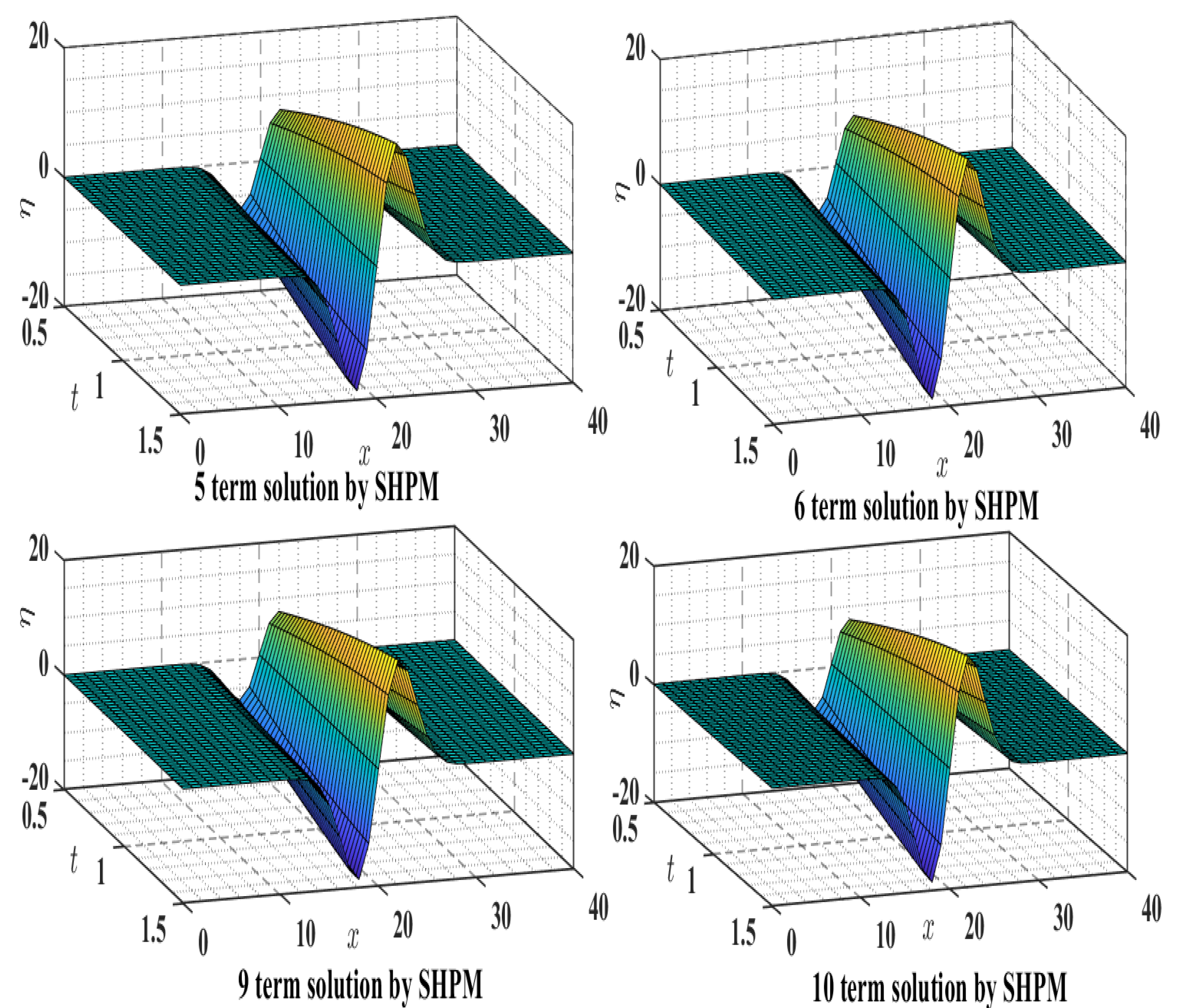
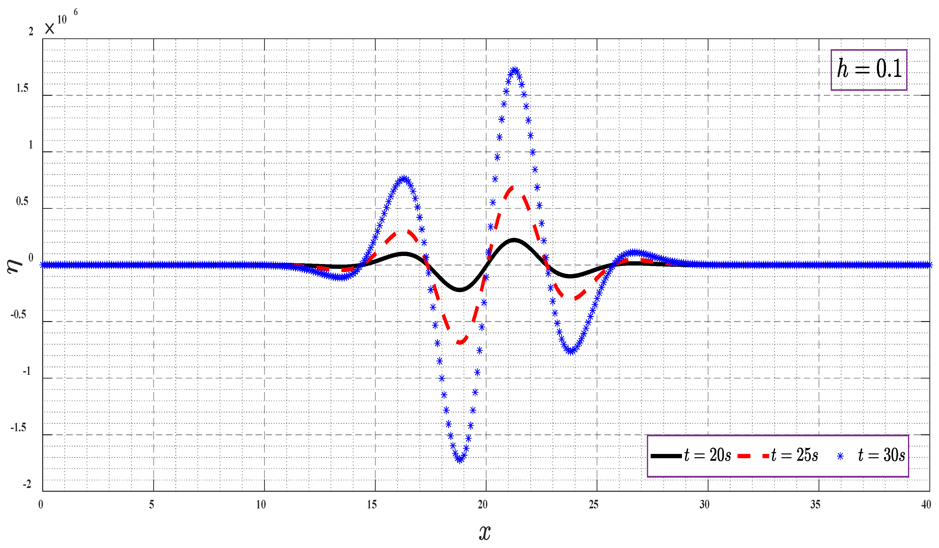
Figure 2 shows the term-wise solution of the SWWE (7) with SHPM at a fixed . As seen in Figure 2, the proposed technique converges as the number of terms increases. The WSEs () of SWWEs in one dimension are depicted for various time levels in Figure 3 and Figure 4 with fixed water depth. Figure 3 shows the WSE vs. global coordinate for three distinct time levels (, , and ) whereas Figure 4 shows the WSE vs. global coordinate for time levels , , and . It may be noted from these figures that, as time passes, the WSE also increases, and the thickness of the water wave decreases.
Figure 5 and Figure 6 demonstrate how the amplitude of SWWE changes as the water depth changes from to over two distinct time periods and seconds, respectively. It can be seen in Table 3 that the amplitude of the shallow water wave or WSE increases rapidly when the water depth () increases from 0.1 to 0.2 at a fixed time . Similar observations can be found for . Additionally, when time is increased from to , the WSE fluctuates at a fixed water depth . Similarly, we get comparable results for . Based on these results, it is clear that the nature of SWW by the present method is well validated.
6.2. SHPM vs. HPM [41]
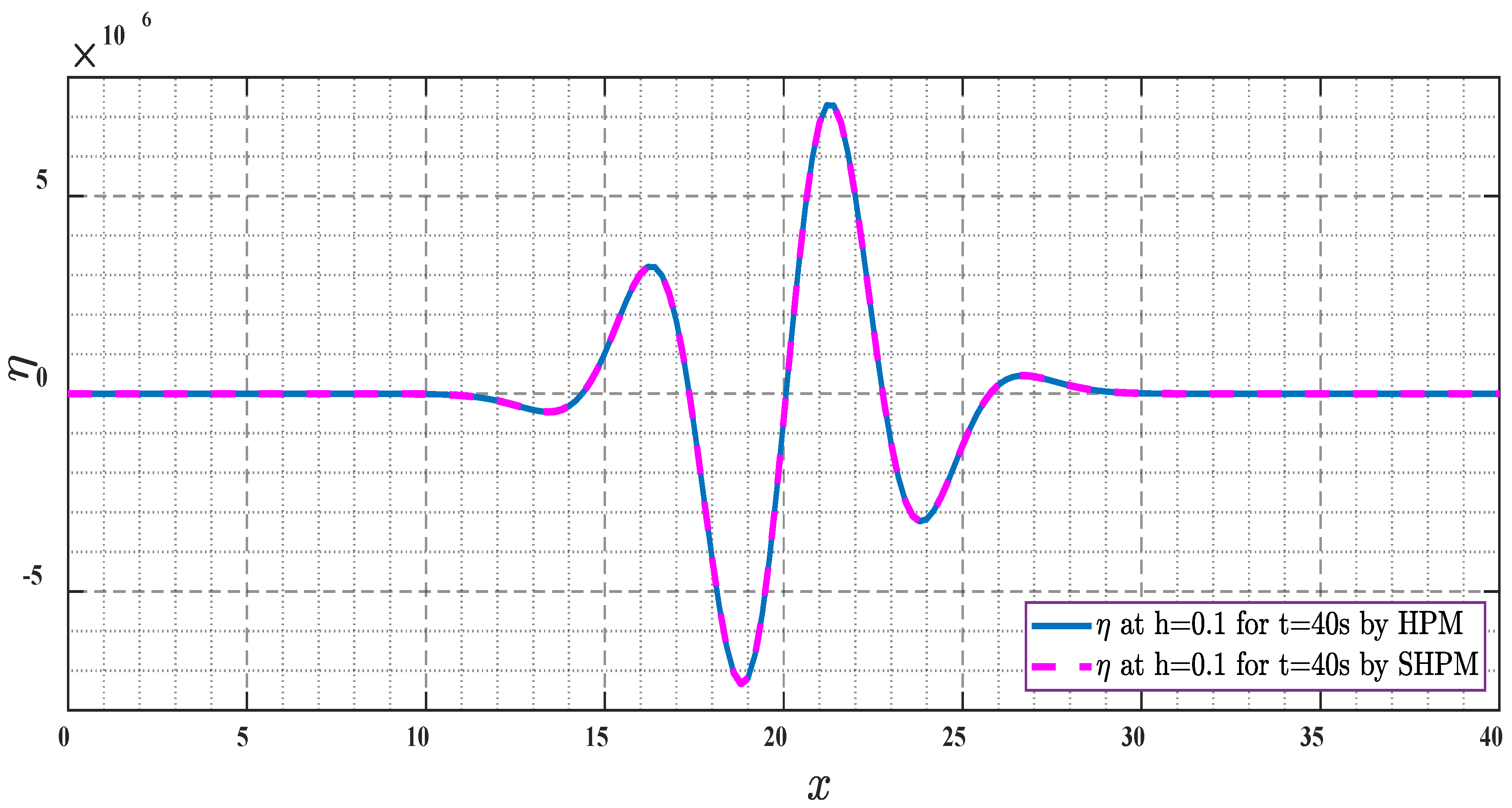
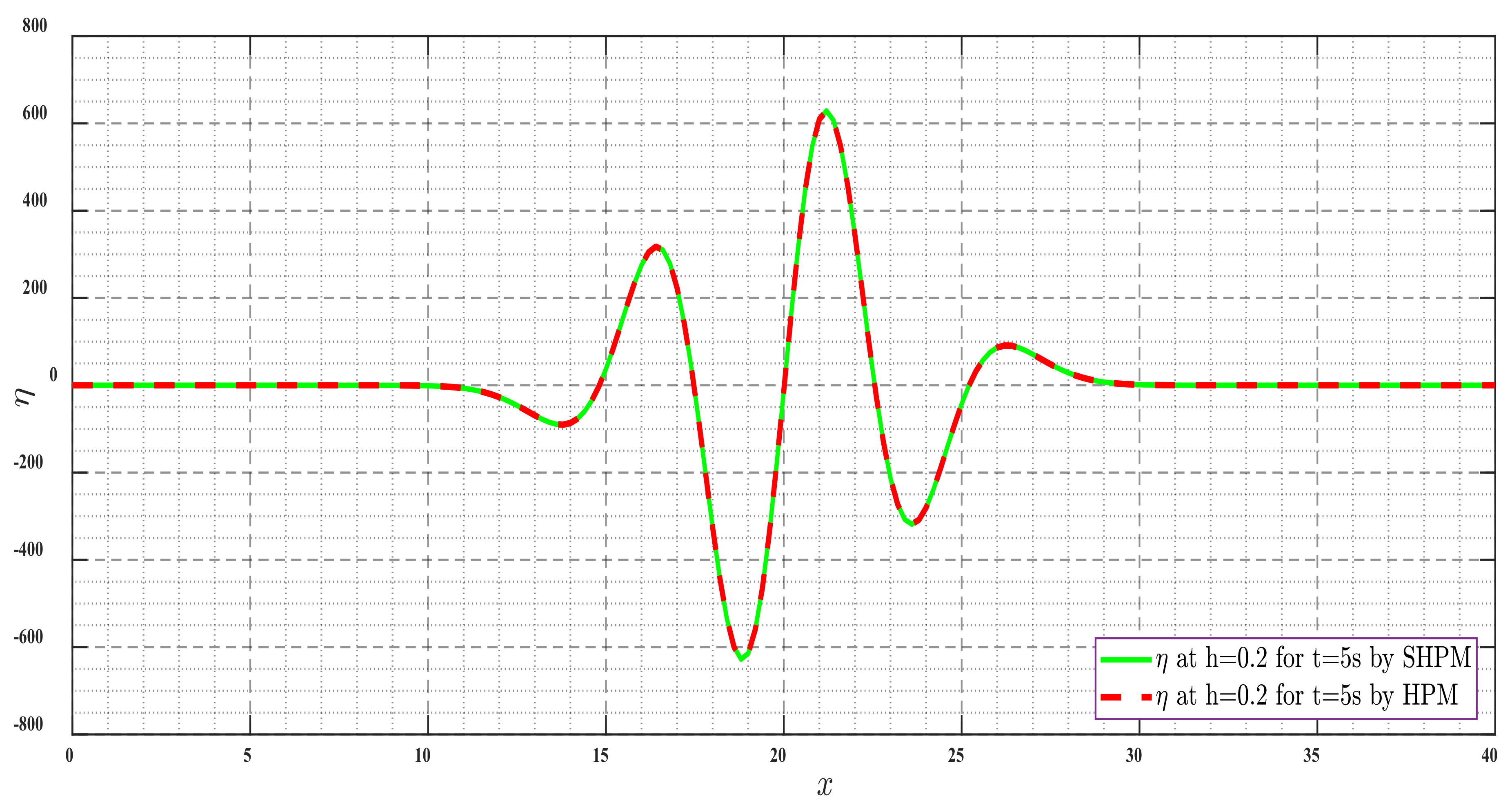
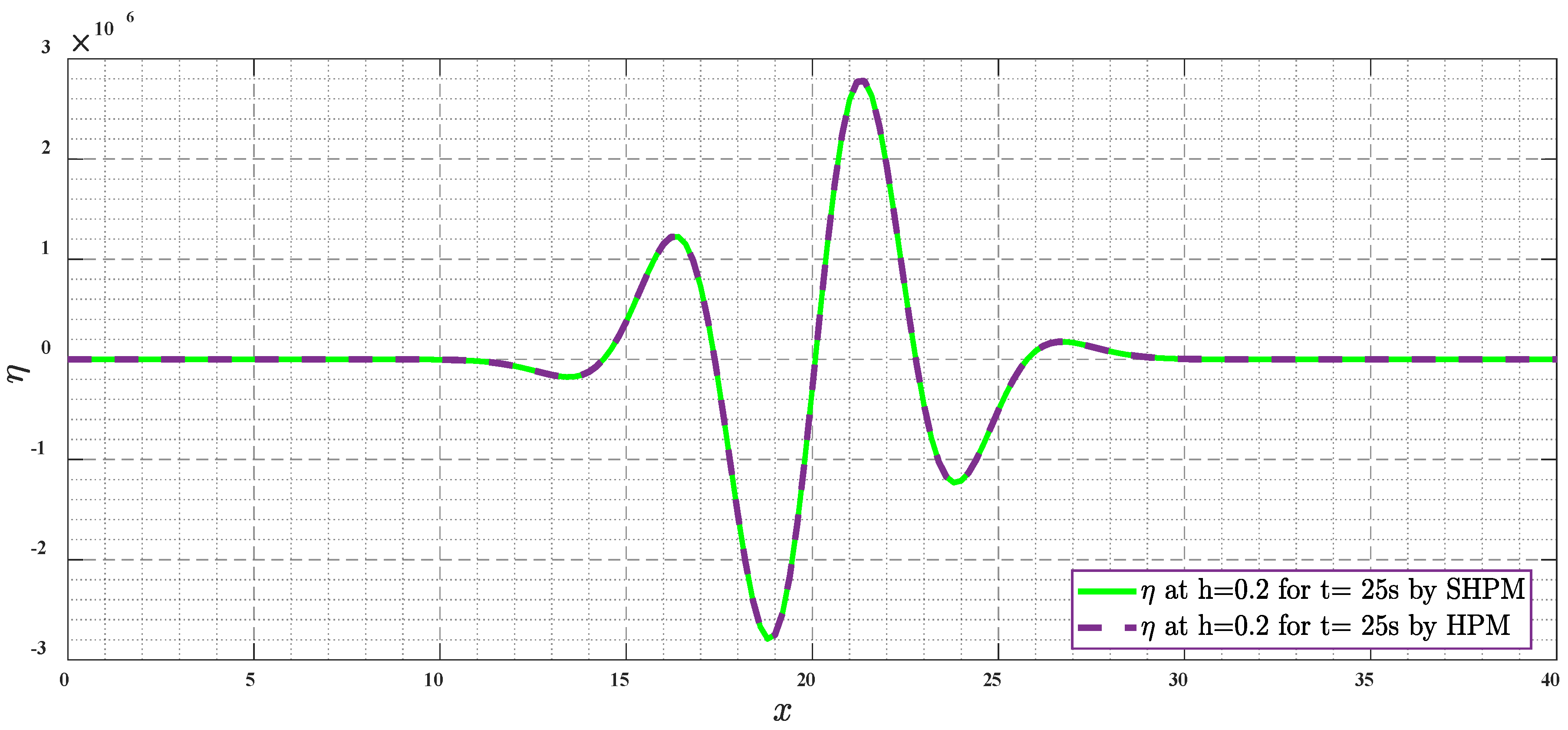
Table 4 compares the term-wise solutions of the SWWE derived by SHPM and HPM for fixed and . As can be seen, SHPM’s approach is in good agreement with HPM [41]. In addition, from Figure 7, Figure 8, Figure 9 and Figure 10, one can see a comparison graph between SHPM and HPM for water surface elevation of the SWWE at fixed water depth for various time levels (, , , and ) and from Figure 11 and Figure 12 for fixed water depth for time levels and , respectively.
6.3. Results Obtained by SHPM in Fuzzy Environment
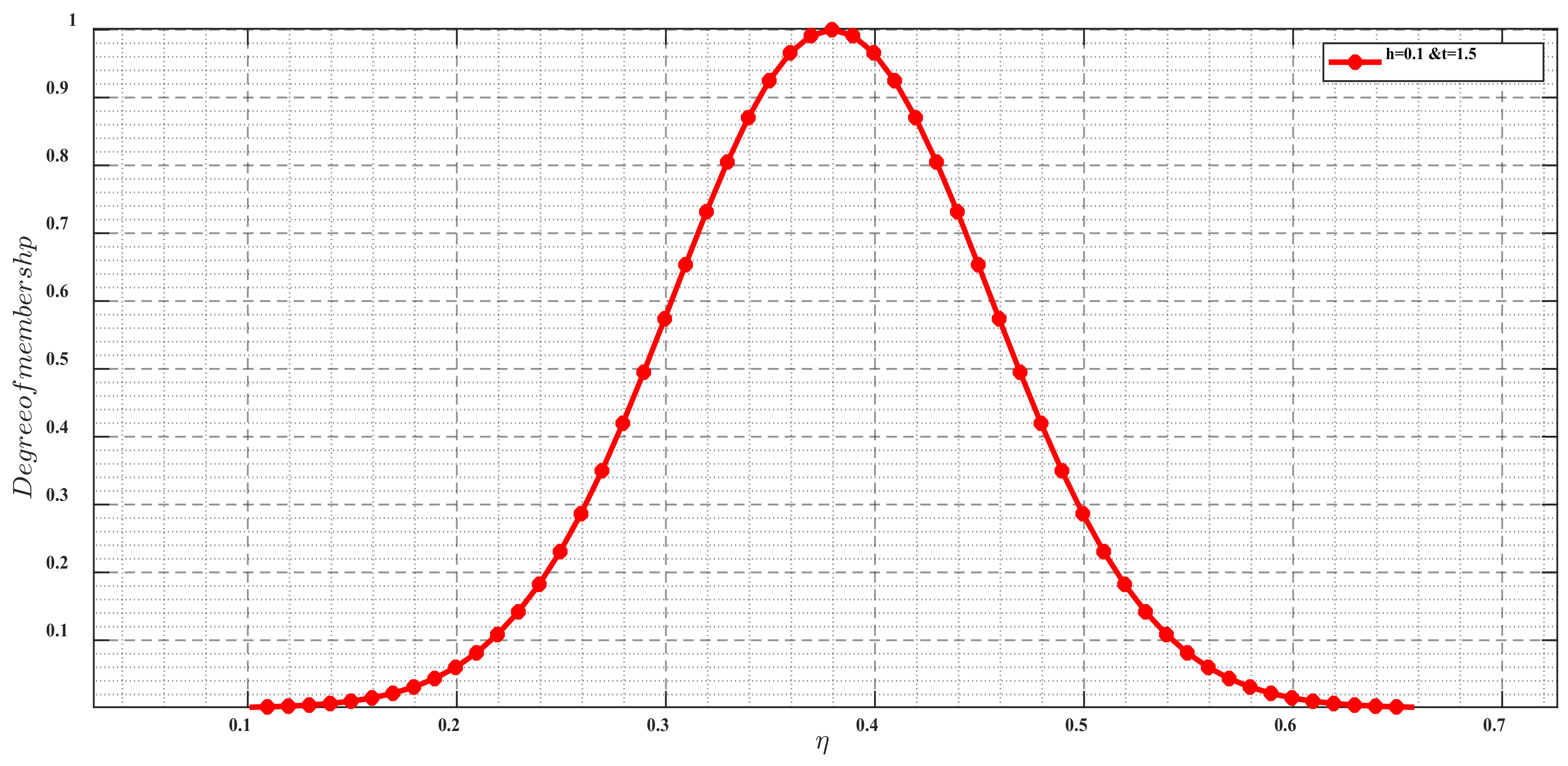
In this section, we discussed the results obtained by SHPM using SGFN. Initially, the fuzzy solution of is depicted in Figure 13. Distinct intervals are generated for different values of and by using the double parametric concept, and in Table 5, the lower value (LV) and upper value (UV) are estimated for the fuzzy solution of . Furthermore, by fixing the value of global coordinate , the investigation is carried out in three different ways as below:
- taking fixed water depth at different time levels ,
- taking fixed time level with a variation in water depth ,
- varying both time and water depth of shallow water waves.
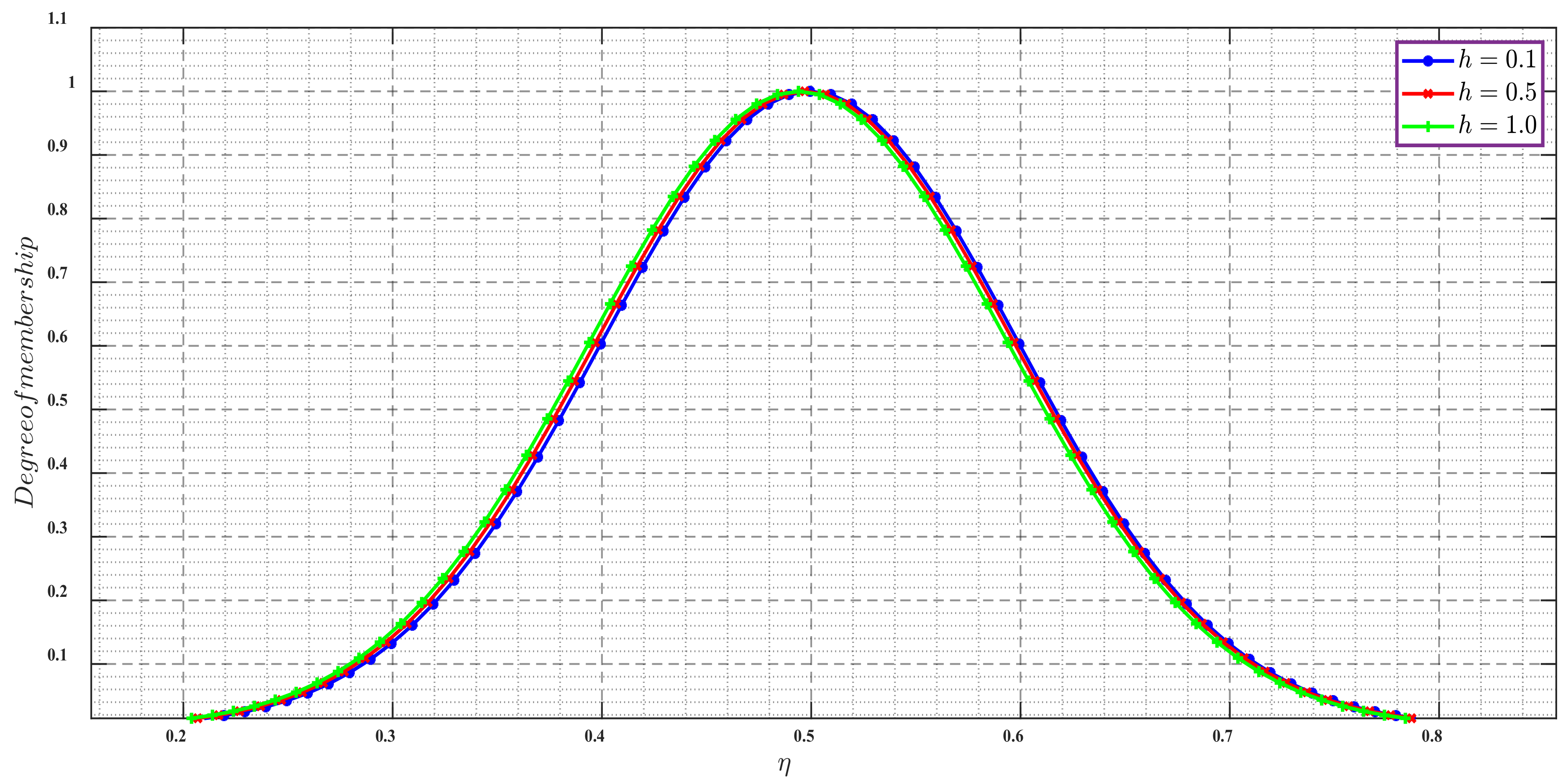
Table 6 shows the fuzzy solution of for different values of and for fixed and at various time levels ( and ). Likewise, Figure 14 shows the corresponding results and it may be observed that as time increases from 0.2 s to 1 s, the width of the fuzzy shallow water wave gradually decreases. Similarly, Figure 15 shows the behavior of the FSWWE for fixed and with various water depths , and . Corresponding fuzzy solutions for different values of and are listed in Table 7. Finally, in Table 8 a comparison is given between two different water depths ( and ) for two different time levels ( and ) at a fixed value. From this observation, one may see that along the direction, when we fixed the value of , there is a variation in the width of the water wave when time is increasing from to for as well as .
7. Conclusions
In this paper, SHPM was used to solve SWWEs in both crisp and fuzzy environments. SHPM offers a solution in the form of a convergent series. The obtained results are found to be in excellent agreement with HPM [41]. The results of both methods are graphically compared. The main advantage of this method over HPM is that it is a powerful and efficient method for determining analytical solutions to wave equations. SWWEs with fuzzy initial conditions are solved using SHPM with the help of a parametric form. Results of FSWWEs are presented in the form of GFN. Based on our obtained results, it is clear that the nature of SWE by the present method is well validated. The present conclusion of linear shallow water waves may be inspiring because these may be useful for future research in other areas.
Author Contributions
Conceptualization, M.S.; Methodology, M.S.; Supervision, S.C.; Writing—original draft, M.S.; Writing—review & editing, S.C. All authors have read and agreed to the published version of the manuscript.
Funding
This research received no external funding.
Institutional Review Board Statement
Not applicable.
Informed Consent Statement
Not applicable.
Data Availability Statement
Data sharing not applicable.
Acknowledgments
The first author is thankful to the University Grants Commission (UGC), New Delhi, India for the financial support to carry out the present research work.
Conflicts of Interest
The authors declare no conflict of interest.
Abbreviations
| ST | Sawi transform |
| GFN | Gaussian fuzzy numbers |
| SGFN | symmetric Gaussian fuzzy numbers |
| SWWs | Shallow water waves |
| SWWEs | shallow water wave equations |
| FSWWEs | fuzzy shallow water wave equations |
| WSE | water surface elevation |
| FEM | Finite Element Method |
| VIM | variational iteration method |
| FVM | Finite Volume Method |
| FDM | Finite Difference Method |
| ADM | Adomian decomposition method |
| HPM | homotopy perturbation method |
| FRDTM | fractional reduced differential transform method |
| SHPM | Sawi transform based homotopy perturbation method |
References
- Safari, M. Analytical Solution of Two Extended Model Equations for Shallow Water Waves by Adomian’s Decomposition Method. Adv. Pure Math. 2011, 1, 238–242. [Google Scholar] [CrossRef]
- Benkhaldoun, F.; Seaid, M. A simple finite volume method for the shallow water equations. J. Comput. Appl. Math. 2010, 234, 58–72. [Google Scholar] [CrossRef]
- Busto, S.; Dumbser, M. A staggered semi-implicit hybrid finite volume/finite element scheme for the shallow water equations at all Froude numbers. Appl. Numer. Math. 2022, 175, 108–132. [Google Scholar] [CrossRef]
- Carfora, M.F. Effectiveness of the operator splitting for solving the atmospherical shallow water equations. Int. J. Numer. Methods Heat Fluid Flow 2001, 11, 213–226. [Google Scholar] [CrossRef]
- Wu, N.-J.; Chen, C.; Tsay, T.-K. Application of weighted-least-square local polynomial approximation to 2D shallow water equation problems. Eng. Anal. Bound. Elements 2016, 68, 124–134. [Google Scholar] [CrossRef]
- Cho, Y.-S.; Sohn, D.-H.; Lee, S.O. Practical modified scheme of linear shallow-water equations for distant propagation of tsunamis. Ocean Eng. 2007, 34, 1769–1777. [Google Scholar] [CrossRef]
- Liu, Y.; Shi, Y.; Yuen, D.A.; Sevre, E.O.D.; Yuan, X.; Xing, H.L. Comparison of linear and nonlinear shallow wave water equations applied to tsunami waves over the China Sea. Acta Geotech. 2008, 4, 129–137. [Google Scholar] [CrossRef]
- Tandel, P.; Patel, H.; Patel, T. Tsunami wave propagation model: A fractional approach. J. Ocean Eng. Sci. 2021. [Google Scholar] [CrossRef]
- Patel, T.; Patel, H.; Meher, R. Analytical study of atmospheric internal waves model with fractional approach. J. Ocean Eng. Sci. 2022. [Google Scholar] [CrossRef]
- Patel, H.; Patel, T.; Pandit, D. An efficient technique for solving fractional-order diffusion equations arising in oil pollution. J. Ocean Eng. Sci. 2022. [Google Scholar] [CrossRef]
- Patel, H.S.; Patel, T. Applications of Fractional Reduced Differential Transform Method for Solving the Generalized Fractional-order Fitzhugh–Nagumo Equation. Int. J. Appl. Comput. Math. 2021, 7, 188. [Google Scholar] [CrossRef]
- Patel, T.; Patel, H. An analytical approach to solve the fractional-order (2 + 1)-dimensional Wu–Zhang equation. Math. Methods Appl. Sci. 2022. [Google Scholar] [CrossRef]
- He, J.-H. Variational iteration method—A kind of non-linear analytical technique: Some examples. Int. J. Non-linear Mech. 1999, 34, 699–708. [Google Scholar] [CrossRef]
- Wazwaz, A.-M. The variational iteration method for solving linear and nonlinear systems of PDEs. Comput. Math. Appl. 2007, 54, 895–902. [Google Scholar] [CrossRef]
- Wazwaz, A.-M. A study on linear and nonlinear Schrodinger equations by the variational iteration method. Chaos Solitons Fractals 2008, 37, 1136–1142. [Google Scholar] [CrossRef]
- Wang, K.-L. Exact solitary wave solution for fractal shallow water wave model by He’s variational method. Mod. Phys. Lett. B 2022, 36, 2150602. [Google Scholar] [CrossRef]
- Mansfield, E.L.; Clarkson, P.A. Symmetries and exact solutions for a 2 þ 1-dimensional shallow water wave equation. Math. Comput. Simul. 1997, 43, 39–55. [Google Scholar] [CrossRef]
- Bernetti, R.; Titarev, V.; Toro, E. Exact solution of the Riemann problem for the shallow water equations with discontinuous bottom geometry. J. Comput. Phys. 2008, 227, 3212–3243. [Google Scholar] [CrossRef]
- Wazwaz, A.-M. Multiple-soliton solutions of two extended model equations for shallow water waves. Appl. Math. Comput. 2008, 201, 790–799. [Google Scholar] [CrossRef]
- Wazwaz, A.-M. The Hirota’s direct method for multiple-soliton solutions for three model equations of shallow water waves. Appl. Math. Comput. 2007, 201, 489–503. [Google Scholar] [CrossRef]
- LeFloch, P.G.; Thanh, M.D. A Godunov-type method for the shallow water equations with discontinuous topography in the resonant regime. J. Comput. Phys. 2011, 230, 7631–7660. [Google Scholar] [CrossRef]
- Bekir, A.; Aksoy, E. Exact solutions of extended shallow water wave equations by exp-function method. Int. J. Numer. Methods Heat Fluid Flow 2013, 23, 305–319. [Google Scholar] [CrossRef]
- Gu, J.; Zhang, Y.; Dong, H. Dynamic behaviors of interaction solutions of (3+1)-dimensional Shallow Water wave equation. Comput. Math. Appl. 2018, 76, 1408–1419. [Google Scholar] [CrossRef]
- Xin, X.; Zhang, L.; Xia, Y.; Liu, H. Nonlocal symmetries and exact solutions of the (2+1)-dimensional generalized variable coefficient shallow water wave equation. Appl. Math. Lett. 2019, 94, 112–119. [Google Scholar] [CrossRef]
- Wang, K. Fractal Solitary Wave Solutions for Fractal Nonlinear Dispersive Boussinesq-Like Models. Fractals 2022, 30, 1–8. [Google Scholar] [CrossRef]
- Clements, D.L.; Rogers, C. Analytic solution of the linearized shallow-water wave equations for certain continuous depth variations. J. Aust. Math. Soc. Ser. B Appl. Math. 1975, 19, 81–94. [Google Scholar] [CrossRef]
- Baskonus, H.M.; Eskitascioglu, E.I. Complex Wave Surfaces to the Extended Shallow Water Wave Model with (2 1)-dimensional. Comput. Methods Differ. Equ. 2020, 8, 585–596. [Google Scholar] [CrossRef]
- Noeiaghdam, L.; Sidorov, D. Dynamical control on the homotopy analysis method for solving nonlinear shallow water wave equation. J. Phys. Conf. Ser. 2021, 1847, 012010. [Google Scholar] [CrossRef]
- Adeyemo, O.D.; Khalique, C.M. Stability analysis, symmetry solutions and conserved currents of a two-dimensional extended shallow water wave equation of fluid mechanics. Partial Differ. Equ. Appl. Math. 2021, 4, 100134. [Google Scholar] [CrossRef]
- Stynes, M.; Stynes, D. Convection-diffusion problems. Am. Math. Soc. 2018, 196, 15–84. [Google Scholar]
- Salnikov, N.N.; Siryk, S.V.; Tereshchenko, I.A.; Siryk, S. On Construction of Finite-Dimensional Mathematical Model of Convection-Diffusion Process with Usage of the Petrov-Galerkin Method. J. Long-Term Eff. Med. Implant. 2010, 42, 67–83. [Google Scholar] [CrossRef]
- Siryk, S.V.; Salnikov, N.N. Numerical Solution of Burgers’ Equation by Petrov-Galerkin Method with Adaptive Weighting Functions. J. Autom. Inf. Sci. 2012, 44, 50–67. [Google Scholar] [CrossRef]
- Salnikov, N.N.; Siryk, S.V. Construction of Weight Functions of the Petrov–Galerkin Method for Convection–Diffusion–Reaction Equations in the Three-Dimensional Case. Cybern 2014, 50, 805–814. [Google Scholar] [CrossRef]
- John, V.; Knobloch, P.; Novo, J. Finite elements for scalar convection-dominated equations and incompressible flow problems: A never ending story? Comput. Vis. Sci. 2018, 19, 47–63. [Google Scholar] [CrossRef]
- He, J.-H. Homotopy perturbation technique. Comput. Methods Appl. Mech. Eng. 1999, 178, 257–262. [Google Scholar] [CrossRef]
- Chen, Y.; An, H. Homotopy perturbation method for a type of nonlinear coupled equations with parameters derivative. Appl. Math. Comput. 2008, 204, 764–772. [Google Scholar] [CrossRef]
- Hemeda, A.A. Homotopy Perturbation Method for Solving Systems of Nonlinear Coupled Equations. Appl. Math. Sci. 2012, 6, 4787–4800. [Google Scholar]
- Sheikholeslami, M.; Hatami, M.; Ganji, D. Micropolar fluid flow and heat transfer in a permeable channel using analytical method. J. Mol. Liq. 2014, 194, 30–36. [Google Scholar] [CrossRef]
- Kumar, S.; Odibat, Z.; Aldhaifallah, M.; Nisar, K.S. A comparison study of two modified analytical approach for the solution of nonlinear fractional shallow water equations in fluid flow. AIMS Math. 2020, 5, 3035–3055. [Google Scholar] [CrossRef]
- Singh, R.; Singh, S.; Wazwaz, A.-M. A modified homotopy perturbation method for singular time dependent Emden–Fowler equations with boundary conditions. J. Math. Chem. 2016, 54, 918–931. [Google Scholar] [CrossRef]
- Karunakar, P.; Chakraverty, S. Comparison of solutions of linear and non-linear shallow water wave equations using homotopy perturbation method. Int. J. Numer. Methods Heat Fluid Flow 2017, 27, 2015–2029. [Google Scholar] [CrossRef]
- Dubey, S.; Chakraverty, S. Solution of Fractional Wave Equation by Homotopy Perturbation Method. InWave Dyn. 2022, 263–277. [Google Scholar] [CrossRef]
- Karunakar, P.; Chakraverty, S. Solution of Interval-Modified Kawahara Differential Equations using Homotopy Perturbation Transform Method. InWave Dyn. 2022, 193–202. [Google Scholar] [CrossRef]
- Mahgoub, M.A.; Mohand, M. The new integral transform Sawi Transform. Adv. Theor. Appl. Math. 2019, 14, 81–87. [Google Scholar]
- Karunakar, P.; Chakraverty, S. 2-D Shallow Water Wave Equations with Fuzzy Parameters; Springer: Singapore, 2018; pp. 1–22. [Google Scholar] [CrossRef]
- Karunakar, P.; Chakraverty, S. Solving shallow water equations with crisp and uncertain initial conditions. Int. J. Numer. Methods Heat Fluid Flow 2018, 28, 2801–2815. [Google Scholar] [CrossRef]
- Chakraverty, S.; Sahoo, D.M.; Mahato, N.R. Fuzzy Numbers. In Concepts of Soft Computing; Springer: Singapore, 2019; pp. 53–69. [Google Scholar] [CrossRef]
- Chakraverty, S.; Tapaswini, S.; Behera, D. Fuzzy Differential Equations and Applications for Engineers and Scientists; CRC Press: Boca Raton, FL, USA, 2016. [Google Scholar]
- Abdelrahim, M.M.; Hassan, A.K. The Use of Adomian Decomposition Method for Solving Nonlinear Wave-Like Equation with Variable Coefficients. Int. J. Math. Its Appl. 2020, 8, 177–186. [Google Scholar]
Figure 1.
Gaussian Fuzzy Number.

Figure 2.
Term-wise solution obtained by SHPM.

Figure 3.
WSE () of SWWE at , , and ().

Figure 4.
WSE () of SWWE at , , and ().

Figure 5.
WSE () of SWWE for and at .

Figure 6.
WSE () of SWWE for and at .

Figure 7.
WSE () by SHPM and HPM at ().

Figure 8.
WSE () by SHPM and HPM at ().

Figure 9.
WSE () by SHPM and HPM at ().

Figure 10.
WSE () by SHPM and HPM at ().

Figure 11.
WSE () by SHPM and HPM at ().

Figure 12.
WSE () by SHPM and HPM at ().

Figure 13.
Fuzzy solution of by SHPM at ().

Figure 14.
Fuzzy solution of by SHPM for .

Figure 15.
Fuzzy solution of by SHPM at .


Table 1.
ST of frequently encountered functions.
| S. N | ||
|---|---|---|
| 1 | 1 | |
| 2 | 1 | |
| 3 | ||
| 4 | ||
| 5 |
Table 2.
Inverse ST of Frequently Encountered Functions.
| S. N | ||
|---|---|---|
| 1 | 1 | |
| 2 | 1 | |
| 3 | ||
| 4 | ||
| 5 |
Table 3.
Amplitude of the shallow water wave.
| 20.2 | 213.7706 | 946.0215 | ||
| 20.4 | 422.9694 | |||
| 20.6 | 600.6070 | |||
| 20.8 | 734.1336 | |||
| 21.0 | 815.0200 | |||
| 21.2 | 839.4148 | |||
| 21.4 | 808.3072 | |||
| 21.6 | 727.1947 | |||
| 21.8 | 605.3195 | |||
| 22.0 | 454.5811 | |||
| 22.2 | 288.2655 | |||
Table 4.
Comparison table between SHPM and HPM.
| SHPM for at | |||||||||
| 1st | 2nd | 3rd | 4th | 5th | 6th | 7th | 8th | 9th | |
| 18 | 0.3033 | −7.2784 | −7.2784 | −7.1236 | −7.1237 | −7.1251 | 7.1251 | −7.1251 | −7.1251 |
| 18.5 | 0.3774 | −6.6992 | −6.7043 | −6.5282 | −6.5282 | −6.5303 | −6.5303 | −6.5303 | −6.5303 |
| 19 | 0.4412 | −5.0744 | −5.0845 | −4.9297 | −4.9295 | −4.9317 | −4.9317 | −4.9317 | −4.9317 |
| 19.5 | 0.4846 | −2.5442 | −2.5582 | −2.4673 | −2.4671 | −2.4685 | −2.4685 | −2.4685 | −2.4685 |
| 20 | 0.5000 | 0.5000 | 0.4847 | 0.4847 | 0.4849 | 0.4849 | 0.4849 | 0.4849 | 0.4849 |
| 20.5 | 0.4846 | 3.5135 | 3.4996 | 3.4087 | 3.4089 | 3.4103 | 3.4103 | 3.4103 | 3.4103 |
| 21 | 0.4412 | 5.9569 | 5.9467 | 5.7919 | 5.7920 | 5.7942 | 5.7942 | 5.7942 | 5.7942 |
| 21.5 | 0.3774 | 7.4540 | 7.4490 | 7.2729 | 7.2729 | 7.2750 | 7.2750 | 7.2750 | 7.2750 |
| 22 | 0.3033 | 7.8849 | 7.8849 | 7.7301 | 7.7300 | 7.7314 | 7.7314 | 7.7314 | 7.7314 |
| HPM [41] for at | |||||||||
| 1st | 2nd | 3rd | 4th | 5th | 6th | 7th | 8th | 9th | |
| 18 | 0.3033 | −7.2784 | −7.2784 | −7.1236 | −7.1237 | −7.1251 | 7.1251 | −7.1251 | −7.1251 |
| 18.5 | 0.3774 | −6.6992 | −6.7043 | −6.5282 | −6.5282 | −6.5303 | −6.5303 | −6.5303 | −6.5303 |
| 19 | 0.4412 | −5.0744 | −5.0845 | −4.9297 | −4.9295 | −4.9317 | −4.9317 | −4.9317 | −4.9317 |
| 19.5 | 0.4846 | −2.5442 | −2.5582 | −2.4673 | −2.4671 | −2.4685 | −2.4685 | −2.4685 | −2.4685 |
| 20 | 0.5000 | 0.5000 | 0.4847 | 0.4847 | 0.4849 | 0.4849 | 0.4849 | 0.4849 | 0.4849 |
| 20.5 | 0.4846 | 3.5135 | 3.4996 | 3.4087 | 3.4089 | 3.4103 | 3.4103 | 3.4103 | 3.4103 |
| 21 | 0.4412 | 5.9569 | 5.9467 | 5.7919 | 5.7920 | 5.7942 | 5.7942 | 5.7942 | 5.7942 |
| 21.5 | 0.3774 | 7.4540 | 7.4490 | 7.2729 | 7.2729 | 7.2750 | 7.2750 | 7.2750 | 7.2750 |
| 22 | 0.3033 | 7.8849 | 7.8849 | 7.7301 | 7.7300 | 7.7314 | 7.7314 | 7.7314 | 7.7314 |
Table 5.
Fuzzy solution of for at .
| LV | UV | |
|---|---|---|
| 0.1 | 0.2166 | 0.5423 |
| 0.2 | 0.2433 | 0.5156 |
| 0.3 | 0.2617 | 0.4972 |
| 0.4 | 0.2767 | 0.4822 |
| 0.5 | 0.2901 | 0.4688 |
| 0.6 | 0.3027 | 0.4561 |
| 0.7 | 0.3153 | 0.4435 |
| 0.8 | 0.3287 | 0.4301 |
| 0.9 | 0.3446 | 0.4143 |
| 1.0 | 0.3794 | 0.3794 |
Table 6.
Fuzzy solution of for .
| LV | UV | LV | UV | LV | UV | LV | UV | LV | UV | |
|---|---|---|---|---|---|---|---|---|---|---|
| 0.1 | 0.2826 | 0.7076 | 0.2744 | 0.6871 | 0.2613 | 0.6543 | 0.2440 | 0.6109 | 0.2233 | 0.5592 |
| 0.2 | 0.3175 | 0.6728 | 0.3083 | 0.6533 | 0.2935 | 0.6221 | 0.2741 | 0.5808 | 0.2509 | 0.5317 |
| 0.3 | 0.3415 | 0.6488 | 0.3316 | 0.6300 | 0.3157 | 0.5999 | 0.2948 | 0.5601 | 0.2698 | 0.5127 |
| 0.4 | 0.3611 | 0.6292 | 0.3506 | 0.6109 | 0.3338 | 0.5817 | 0.3117 | 0.5431 | 0.2853 | 0.4972 |
| 0.5 | 0.3785 | 0.6117 | 0.3676 | 0.5940 | 0.3500 | 0.5656 | 0.3268 | 0.5281 | 0.2991 | 0.4834 |
| 0.6 | 0.3950 | 0.5952 | 0.3836 | 0.5780 | 0.3652 | 0.5503 | 0.3410 | 0.5138 | 0.3122 | 0.4704 |
| 0.7 | 0.4115 | 0.5788 | 0.3996 | 0.5620 | 0.3805 | 0.5351 | 0.3552 | 0.4996 | 0.3252 | 0.4574 |
| 0.8 | 0.4290 | 0.5613 | 0.4165 | 0.5450 | 0.3966 | 0.5190 | 0.3703 | 0.4845 | 0.3390 | 0.4436 |
| 0.9 | 0.4497 | 0.5406 | 0.4366 | 0.5249 | 0.4158 | 0.4998 | 0.3882 | 0.4667 | 0.3554 | 0.4272 |
| 1.0 | 0.4951 | 0.4951 | 0.4808 | 0.4808 | 0.4578 | 0.4578 | 0.4274 | 0.4274 | 0.3913 | 0.3913 |
Table 7.
Fuzzy solution of at .
| LV | UV | LV | UV | LV | UV | |
|---|---|---|---|---|---|---|
| 0.1 | 0.2851 | 0.7137 | 0.2837 | 0.7102 | 0.2819 | 0.7059 |
| 0.2 | 0.3202 | 0.6786 | 0.3186 | 0.6753 | 0.3167 | 0.6711 |
| 0.3 | 0.3444 | 0.6544 | 0.3427 | 0.6512 | 0.3406 | 0.6472 |
| 0.4 | 0.3642 | 0.6346 | 0.3624 | 0.6315 | 0.3602 | 0.6276 |
| 0.5 | 0.3818 | 0.6170 | 0.3799 | 0.6140 | 0.3776 | 0.6102 |
| 0.6 | 0.3984 | 0.6003 | 0.3965 | 0.5974 | 0.3941 | 0.5938 |
| 0.7 | 0.4150 | 0.5837 | 0.4130 | 0.5809 | 0.4105 | 0.5773 |
| 0.8 | 0.4327 | 0.5661 | 0.4306 | 0.5633 | 0.4279 | 0.5599 |
| 0.9 | 0.4535 | 0.5452 | 0.4513 | 0.5426 | 0.4486 | 0.5393 |
| 1.0 | 0.4994 | 0.4994 | 0.4969 | 0.4969 | 0.4939 | 0.4939 |
Table 8.
Fuzzy solution of for and .
| LV | UV | LV | UV | LV | UV | LV | UV | |
|---|---|---|---|---|---|---|---|---|
| 0.1 | 0.2768 | 0.6930 | 0.2166 | 0.5423 | 0.2684 | 0.6721 | 0.1635 | 0.4093 |
| 0.2 | 0.3109 | 0.6589 | 0.2433 | 0.5156 | 0.3015 | 0.6390 | 0.1836 | 0.3891 |
| 0.3 | 0.3344 | 0.6354 | 0.2617 | 0.4972 | 0.3243 | 0.6162 | 0.1975 | 0.3753 |
| 0.4 | 0.3536 | 0.6162 | 0.2767 | 0.4822 | 0.3430 | 0.5976 | 0.2088 | 0.3639 |
| 0.5 | 0.3707 | 0.5991 | 0.2901 | 0.4688 | 0.3595 | 0.5810 | 0.2189 | 0.3538 |
| 0.6 | 0.3869 | 0.5829 | 0.3027 | 0.4561 | 0.3752 | 0.5654 | 0.2285 | 0.3443 |
| 0.7 | 0.4030 | 0.5668 | 0.3153 | 0.4435 | 0.3909 | 0.5497 | 0.2380 | 0.3348 |
| 0.8 | 0.4201 | 0.5497 | 0.3287 | 0.4301 | 0.4075 | 0.5331 | 0.2481 | 0.3246 |
| 0.9 | 0.4404 | 0.5294 | 0.3446 | 0.4143 | 0.4271 | 0.5135 | 0.2601 | 0.3127 |
| 1.0 | 0.4849 | 0.4849 | 0.3794 | 0.3794 | 0.4703 | 0.4703 | 0.2864 | 0.2864 |
Publisher’s Note: MDPI stays neutral with regard to jurisdictional claims in published maps and institutional affiliations. |
© 2022 by the authors. Licensee MDPI, Basel, Switzerland. This article is an open access article distributed under the terms and conditions of the Creative Commons Attribution (CC BY) license (https://creativecommons.org/licenses/by/4.0/).
Share and Cite
MDPI and ACS Style
Sahoo, M.; Chakraverty, S. Sawi Transform Based Homotopy Perturbation Method for Solving Shallow Water Wave Equations in Fuzzy Environment. Mathematics 2022, 10, 2900. https://0-doi-org.brum.beds.ac.uk/10.3390/math10162900
AMA Style
Sahoo M, Chakraverty S. Sawi Transform Based Homotopy Perturbation Method for Solving Shallow Water Wave Equations in Fuzzy Environment. Mathematics. 2022; 10(16):2900. https://0-doi-org.brum.beds.ac.uk/10.3390/math10162900
Chicago/Turabian StyleSahoo, Mrutyunjaya, and Snehashish Chakraverty. 2022. "Sawi Transform Based Homotopy Perturbation Method for Solving Shallow Water Wave Equations in Fuzzy Environment" Mathematics 10, no. 16: 2900. https://0-doi-org.brum.beds.ac.uk/10.3390/math10162900
Note that from the first issue of 2016, this journal uses article numbers instead of page numbers. See further details here.