
New Tilt Fractional-Order Integral Derivative with Fractional Filter (TFOIDFF) Controller with Artificial Hummingbird Optimizer for LFC in Renewable Energy Power Grids


Abstract
:1. Introduction
1.1. Literature Survey
1.2. Motivation
- The AHA employs a different biological background compared to other existing metaheuristic optimization algorithms. The AHA optimizer employs three different foraging strategies with three various flight skills inspired by the hummingbird.
- The AHA optimizer uses different strategies for the exploration, and the exploitation stages. The migration foraging strategy of the AHA optimizer guarantees exploration stage in search space. Whereas, the exploitation stage is promoted through the territorial-foraging strategy. In addition, the guided-foraging strategy emphasizes the exploration stage during early stages, and highlights the exploitation stage during later stages.
- The AHA optimizer has its own distinct mechanism of memory updating. Each one of the hummingbirds needs to know the last visit time to other hummingbirds. The visit time information is recorded within the visit table, wherein each one of the hummingbirds can select its desired source of food.
1.3. Contribution
- A new modified load frequency controller (LFC) based on combining the tilt, FOPID, and fractional filter regulators, namely the tilt FO integral-derivative with fractional-filter (TFOIDFF) controller. The combination of three efficient regulators improves the stability performance, fast transients, and mitigation of existing RESs and loading fluctuations.
- A new controller optimization application for the proposed TFOIDFF controller is proposed based on the newly presented bio-inspired artificial hummingbird optimizer algorithm (AHA). The proposed AHA-based optimization process can eliminate the massive training data required and/or complicated mathematical calculations that are required in other methods.
- A decentralized EV controller using the proposed TFOIDFF LFC controller is proposed in this paper. The TFOIDFF achieves both the LFC functionality and EV control functionality.
- Simultaneous determination of optimum proposed TFOIDFF LFC parameters with AHA optimizer is presented in this paper. All the parameters in interconnected power grids are determined jointly to address the objective function that represents the mitigation of existing frequency and tie-line power deviations in the interconnected power grids.
2. Mathematical Models of Interconnected Power Grids with EVs
2.1. Power Grid Structure
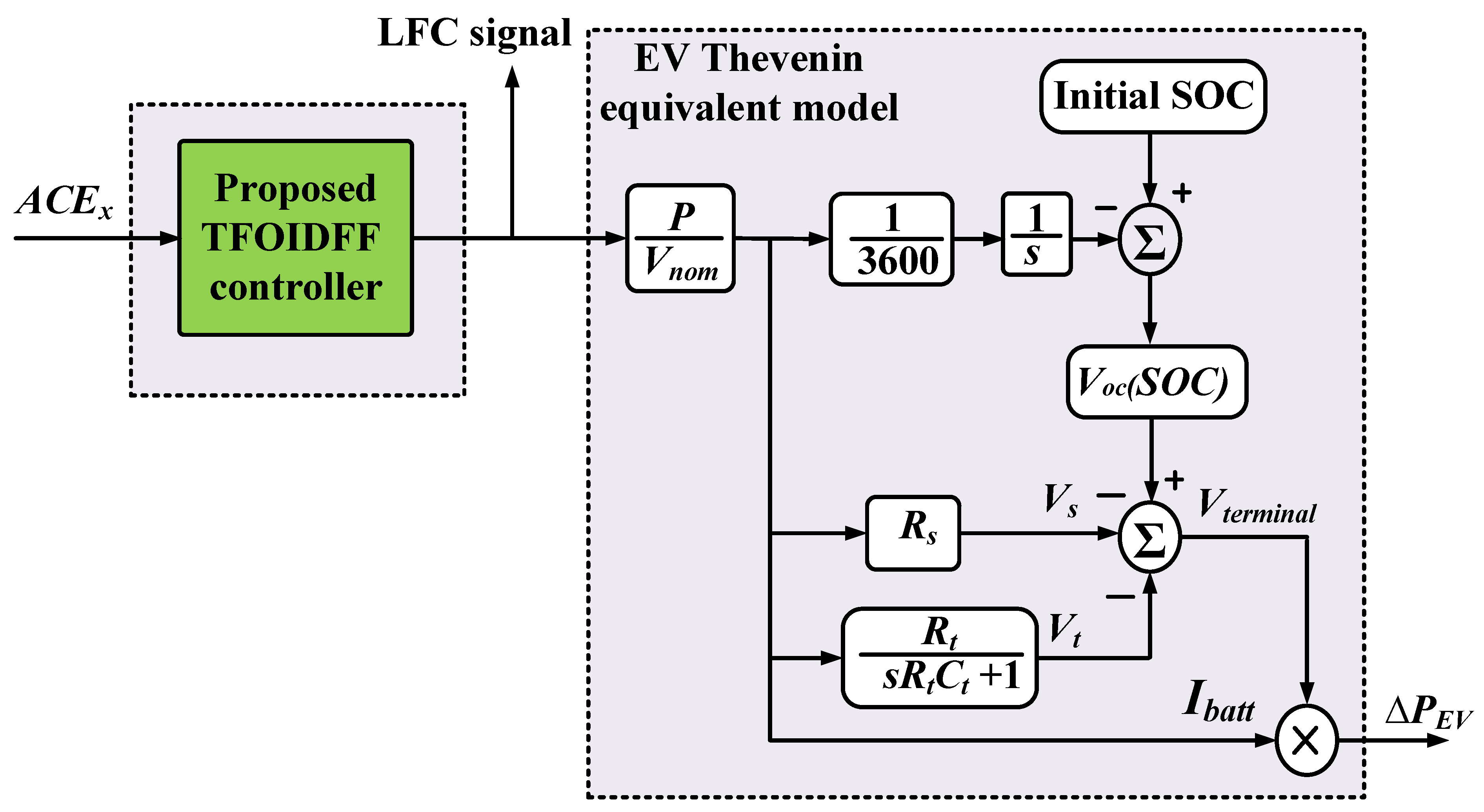
2.2. EV Modeling
2.3. Traditional Energy Source Models
2.4. RESs’ Models
2.5. Complete System State-Space Model
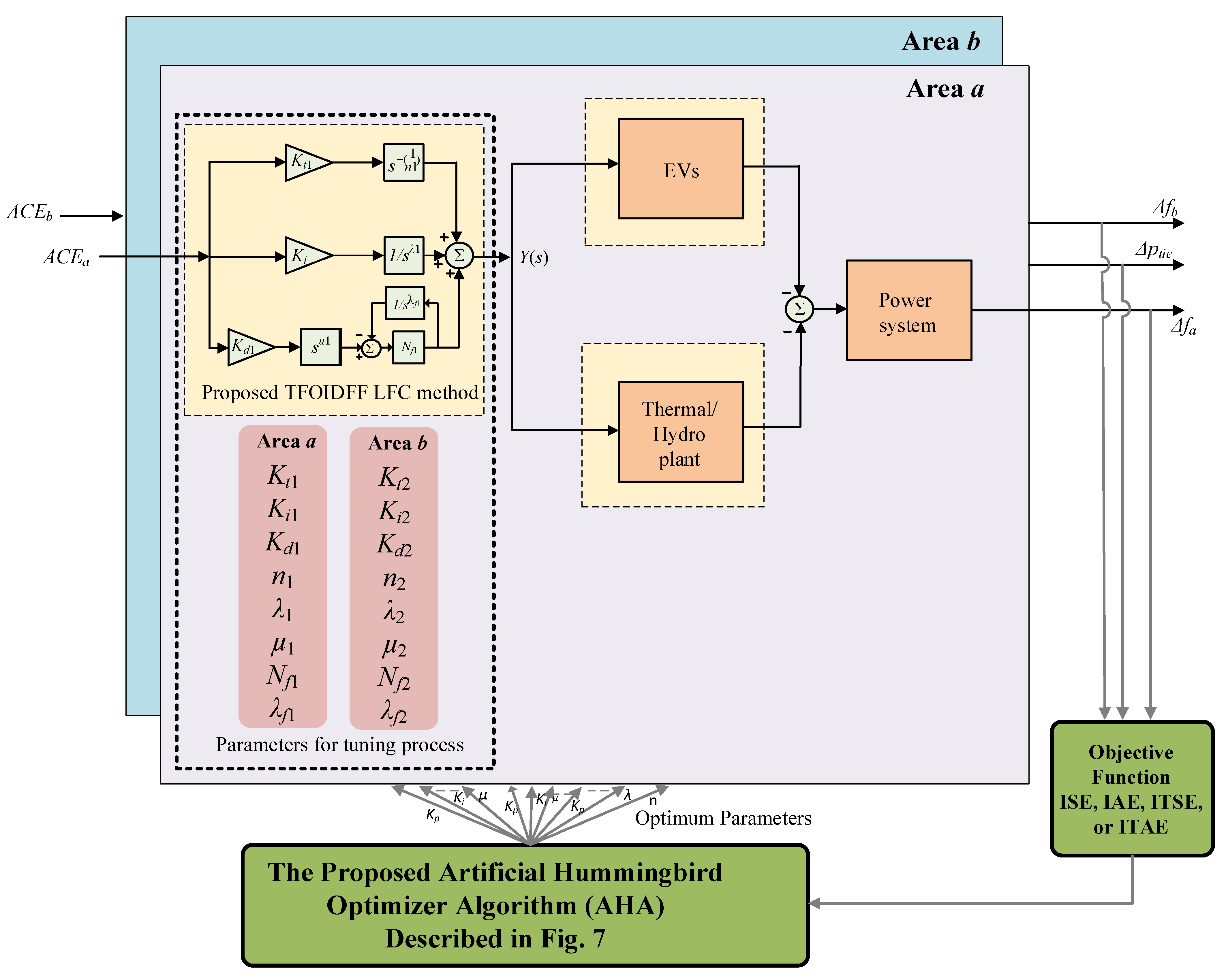
3. The Proposed TFOIDFF Controller
3.1. The FO Calculus Theory
3.2. Existing IO and FO LFC Methods
3.3. The Proposed TFOIDFF Controller
- The use of tilt FO branch instead of IO proportional term adds more flexibility to the design of the proposed TFOIDFF controller. The tilt term can also improve the disturbance-rejection ability and enhance controller robustness against parametric uncertainty.
- The use of FO integrator and derivative FO terms combines the benefits of the FOPID control with the tilt term. The FO ID terms provide more opportunities for flexible design compared with IO-based PID controller. Merging the two controllers adds more flexibility and freedom to the new proposed TFOIDFF controller.
- The use of the fractional filter adds a low-pass filtering property in addition to the FO operator. The use of FF helps at solving the realizability problem of the derivative term. Although the derivative term improves the stability and reduced overshoot response, it amplifies the high-frequency noise. Thus, a filtering stage is needed with the derivative term. Furthermore, the FF helps in mitigating the derivative’s kick effects, which result from instantaneous changes in the input signal of the controller (ACE signals). These effects are eliminated though the employed FF component.
4. The Proposed AHA-Based Parameter Optimization
4.1. Optimization Process of the Proposed TFOIDFF Controller
4.2. The Artificial Hummingbird Optimizer
4.2.1. The Guided Foraging
4.2.2. The Territorial Foraging
4.2.3. The Migration Foraging
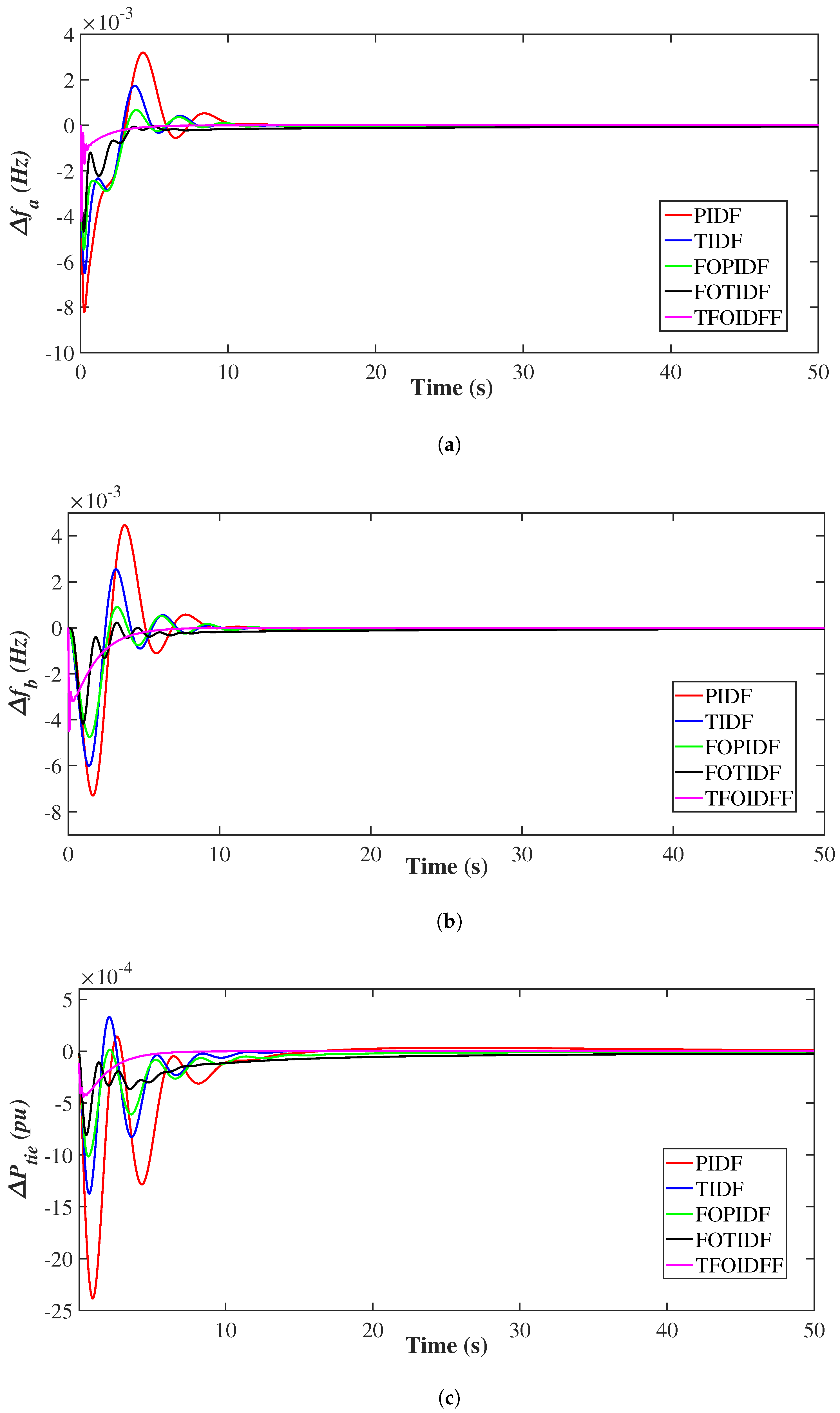
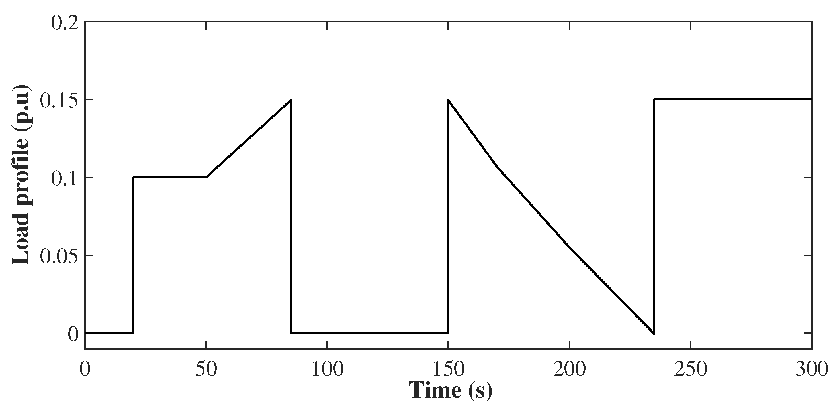
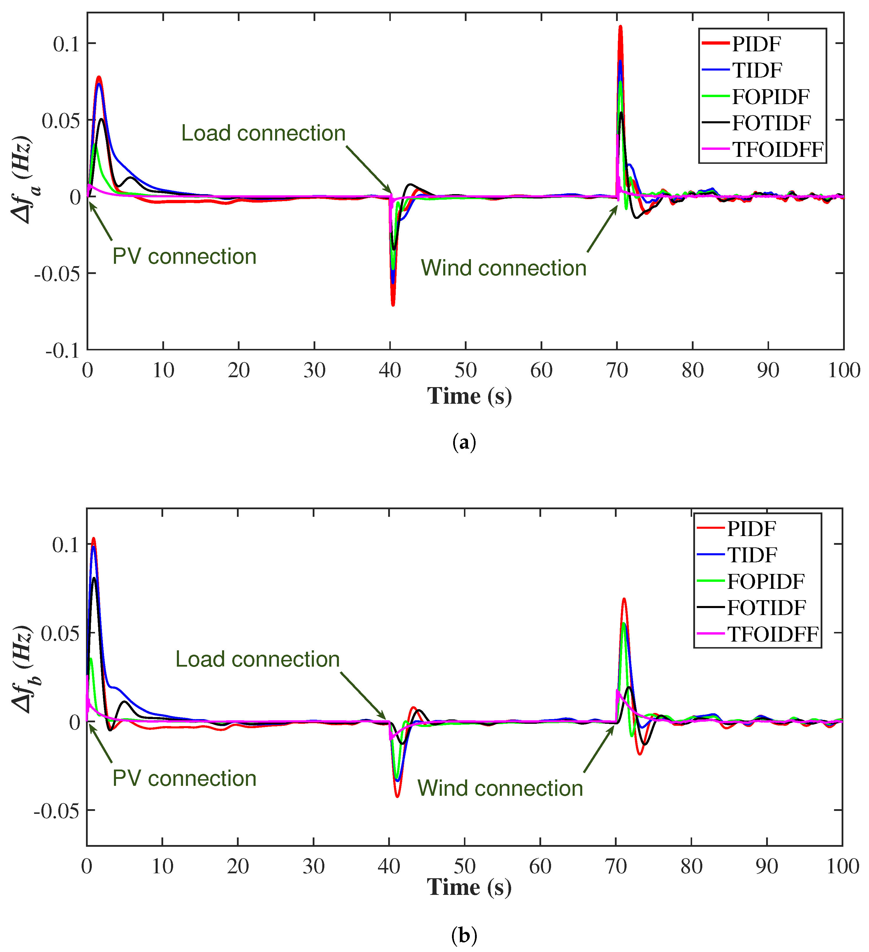
5. Results and Discussions
5.1. Scenario 1
5.2. Scenario 2
5.3. Scenario 3
5.4. Scenario 4
5.5. Scenario 5
5.6. Scenario 6
6. Conclusions
- The proposed TFOIDFF controller demonstrates a more efficient performance than the studied conventional PIDF and TIDF controllers, and the advanced FOPIDF and FOTIDF controllers.
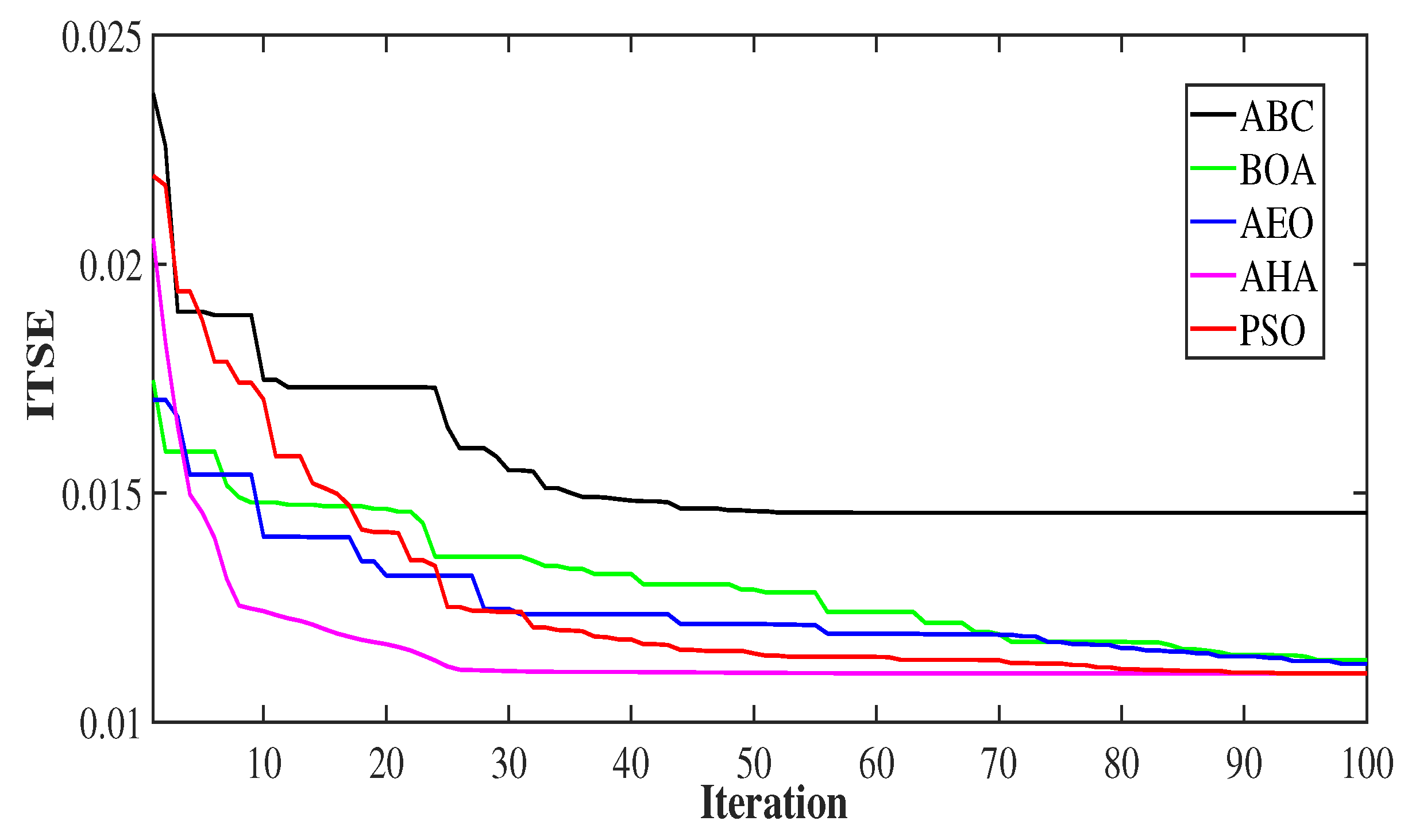
- The obtained comparisons of ISE, ITSE, IAE, and ITAE objective functions verified the faster and better convergence of the proposed AHA method over the ABC, AEO, and BOA optimizers.
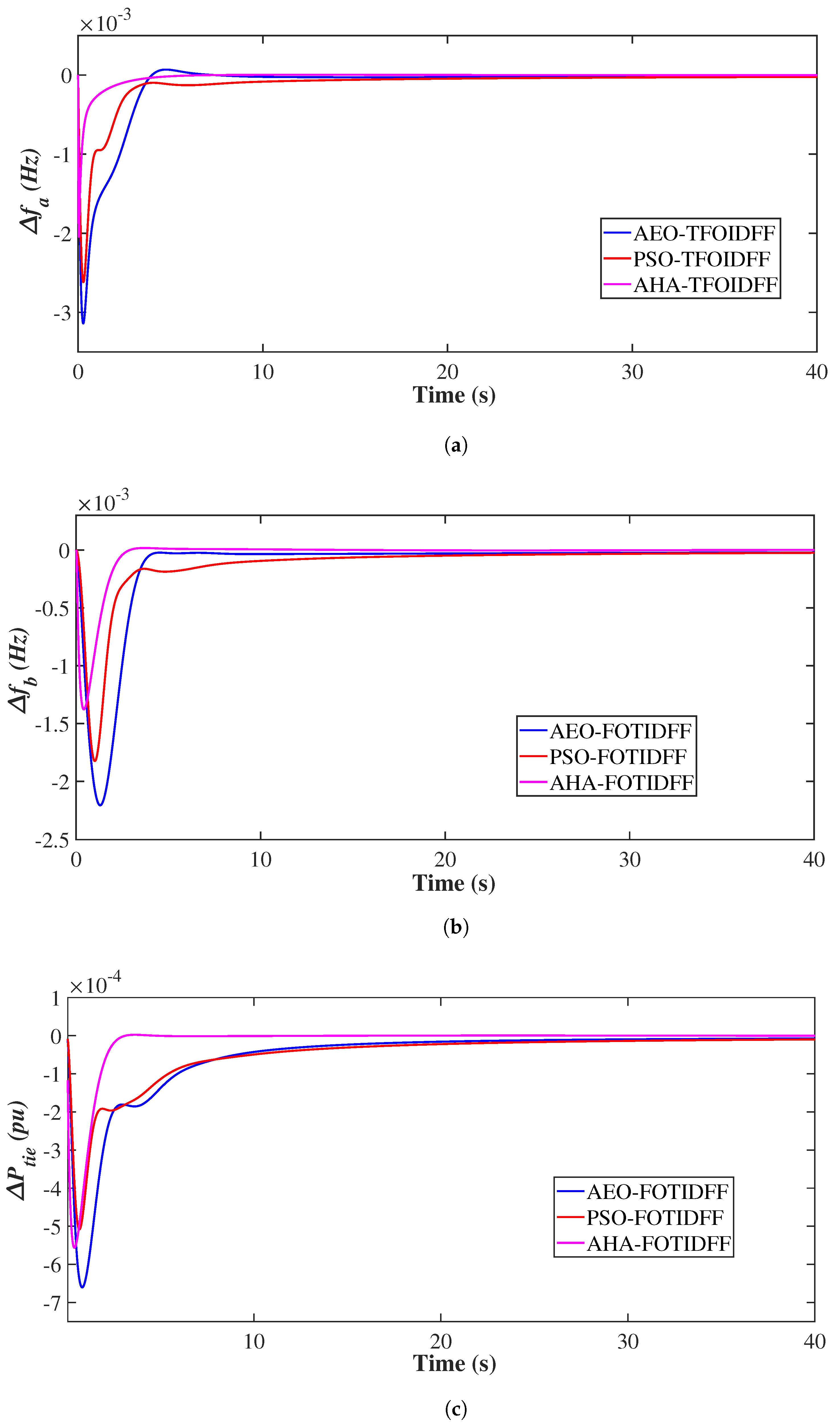
- Moreover, the obtained simulation results proved the minimized frequency, and tie-line power deviation using the proposed optimized TFOIDFF controller compared to existing LFC methods.
- Based on the designed optimized controllers, the coordination of the LFC and installed EVs is achieved to maintain multi-area power system stability during various existing disturbances in power systems.
Author Contributions
Funding
Institutional Review Board Statement
Informed Consent Statement
Data Availability Statement
Conflicts of Interest
References
- Yildirim, B.; Gheisarnejad, M.; Khooban, M.H. A Robust Non-Integer Controller Design for Load Frequency Control in Modern Marine Power Grids. IEEE Trans. Emerg. Top. Comput. Intell. 2022, 6, 852–866. [Google Scholar] [CrossRef]
- Ahmed, E.M.; Mohamed, E.A.; Elmelegi, A.; Aly, M.; Elbaksawi, O. Optimum Modified Fractional Order Controller for Future Electric Vehicles and Renewable Energy-Based Interconnected Power Systems. IEEE Access 2021, 9, 29993–30010. [Google Scholar] [CrossRef]
- Sun, P.; Yun, T.; Chen, Z. Multi-objective robust optimization of multi-energy microgrid with waste treatment. Renew. Energy 2021, 178, 1198–1210. [Google Scholar] [CrossRef]
- Xiao, D.; Chen, H.; Wei, C.; Bai, X. Statistical Measure for Risk-Seeking Stochastic Wind Power Offering Strategies in Electricity Markets. J. Mod. Power Syst. Clean Energy 2021. [Google Scholar] [CrossRef]
- Said, S.M.; Aly, M.; Hartmann, B.; Mohamed, E.A. Coordinated fuzzy logic-based virtual inertia controller and frequency relay scheme for reliable operation of low-inertia power system. IET Renew. Power Gener. 2021, 15, 1286–1300. [Google Scholar] [CrossRef]
- Liu, L.; Hu, Z.; Mujeeb, A. Automatic Generation Control Considering Uncertainties of the Key Parameters in the Frequency Response Model. IEEE Trans. Power Syst. 2022. [Google Scholar] [CrossRef]
- Magdy, G.; Ali, H.; Xu, D. Effective control of smart hybrid power systems: Cooperation of robust LFC and virtual inertia control system. CSEE J. Power Energy Syst. 2021. [Google Scholar] [CrossRef]
- Paliwal, N.; Srivastava, L.; Pandit, M. Application of grey wolf optimization algorithm for load frequency control in multi-source single area power system. Evol. Intell. 2020, 15, 563–584. [Google Scholar] [CrossRef]
- Aryan, P.; Ranjan, M.; Shankar, R. Deregulated LFC scheme using equilibrium optimized Type-2 fuzzy controller. WEENTECH Proc. Energy 2021, 8, 494–505. [Google Scholar] [CrossRef]
- Dreidy, M.; Mokhlis, H.; Mekhilef, S. Inertia response and frequency control techniques for renewable energy sources: A review. Renew. Sustain. Energy Rev. 2017, 69, 144–155. [Google Scholar] [CrossRef]
- Fernández-Guillamón, A.; Gómez-Lázaro, E.; Muljadi, E.; Molina-García, Á. Power systems with high renewable energy sources: A review of inertia and frequency control strategies over time. Renew. Sustain. Energy Rev. 2019, 115, 109369. [Google Scholar] [CrossRef] [Green Version]
- Lv, X.; Sun, Y.; Wang, Y.; Dinavahi, V. Adaptive Event-Triggered Load Frequency Control of Multi-Area Power Systems Under Networked Environment via Sliding Mode Control. IEEE Access 2020, 8, 86585–86594. [Google Scholar] [CrossRef]
- Vrdoljak, K.; Perić, N.; Petrović, I. Sliding mode based load-frequency control in power systems. Electr. Power Syst. Res. 2010, 80, 514–527. [Google Scholar] [CrossRef]
- Pan, C.; Liaw, C. An adaptive controller for power system load-frequency control. IEEE Trans. Power Syst. 1989, 4, 122–128. [Google Scholar] [CrossRef]
- Bu, X.; Yu, W.; Cui, L.; Hou, Z.; Chen, Z. Event-Triggered Data-Driven Load Frequency Control for Multiarea Power Systems. IEEE Trans. Ind. Inform. 2022, 18, 5982–5991. [Google Scholar] [CrossRef]
- Yu, X.; Tomsovic, K. Application of linear matrix inequalities for load frequency control with communication delays. IEEE Trans. Power Syst. 2004, 19, 1508–1515. [Google Scholar] [CrossRef]
- Rakhshani, E.; Rodriguez, P.; Cantarellas, A.M.; Remon, D. Analysis of derivative control based virtual inertia in multi-area high-voltage direct current interconnected power systems. IET Gener. Transm. Distrib. 2016, 10, 1458–1469. [Google Scholar] [CrossRef] [Green Version]
- Kerdphol, T.; Rahman, F.S.; Mitani, Y.; Watanabe, M.; Kufeoglu, S. Robust Virtual Inertia Control of an Islanded Microgrid Considering High Penetration of Renewable Energy. IEEE Access 2018, 6, 625–636. [Google Scholar] [CrossRef]
- Li, X.; Ye, D. Event-Based Distributed Fuzzy Load Frequency Control for Multiarea Nonlinear Power Systems with Switching Topology. IEEE Trans. Fuzzy Syst. 2022. [Google Scholar] [CrossRef]
- Saxena, S.; Hote, Y.V. Load Frequency Control in Power Systems via Internal Model Control Scheme and Model-Order Reduction. IEEE Trans. Power Syst. 2013, 28, 2749–2757. [Google Scholar] [CrossRef]
- Kocaarslan, I.; Çam, E. Fuzzy logic controller in interconnected electrical power systems for load-frequency control. Int. J. Electr. Power Energy Syst. 2005, 27, 542–549. [Google Scholar] [CrossRef]
- Shiroei, M.; Ranjbar, A. Supervisory predictive control of power system load frequency control. Int. J. Electr. Power Energy Syst. 2014, 61, 70–80. [Google Scholar] [CrossRef]
- Pandey, S.K.; Mohanty, S.R.; Kishor, N. A literature survey on load–frequency control for conventional and distribution generation power systems. Renew. Sustain. Energy Rev. 2013, 25, 318–334. [Google Scholar] [CrossRef]
- Shankar, R.; Pradhan, S.; Chatterjee, K.; Mandal, R. A comprehensive state of the art literature survey on LFC mechanism for power system. Renew. Sustain. Energy Rev. 2017, 76, 1185–1207. [Google Scholar] [CrossRef]
- Panda, S.; Mohanty, B.; Hota, P. Hybrid BFOA-PSO algorithm for automatic generation control of linear and nonlinear interconnected power systems. Appl. Soft Comput. 2013, 13, 4718–4730. [Google Scholar] [CrossRef]
- Khokhar, B.; Dahiya, S.; Singh Parmar, K.P. Atom search optimization based study of frequency deviation response of a hybrid power system. In Proceedings of the 2020 IEEE 9th Power India International Conference (PIICON), Sonepat, India, 28 February–1 March 2020; pp. 1–5. [Google Scholar] [CrossRef]
- Sharma, J.; Hote, Y.V.; Prasad, R. PID controller design for interval load frequency control system with communication time delay. Control. Eng. Pract. 2019, 89, 154–168. [Google Scholar] [CrossRef]
- El Yakine Kouba, N.; Menaa, M.; Hasni, M.; Boudour, M. Optimal load frequency control based on artificial bee colony optimization applied to single, two and multi-area interconnected power systems. In Proceedings of the 2015 3rd International Conference on Control, Engineering & Information Technology (CEIT), Tlemcen, Algeri, 25–27 May 2015; pp. 1–6. [Google Scholar] [CrossRef]
- Yousri, D.; Babu, T.S.; Fathy, A. Recent methodology based Harris Hawks optimizer for designing load frequency control incorporated in multi-interconnected renewable energy plants. Sustain. Energy Grids Netw. 2020, 22, 100352. [Google Scholar] [CrossRef]
- Dahab, Y.A.; Abubakr, H.; Mohamed, T.H. Adaptive Load Frequency Control of Power Systems Using Electro-Search Optimization Supported by the Balloon Effect. IEEE Access 2020, 8, 7408–7422. [Google Scholar] [CrossRef]
- Shiva, C.; Shankar, G.; Mukherjee, V. Automatic generation control of power system using a novel quasi-oppositional harmony search algorithm. Int. J. Electr. Power Energy Syst. 2015, 73, 787–804. [Google Scholar] [CrossRef]
- Mohanty, B.; Panda, S.; Hota, P.K. Controller parameters tuning of differential evolution algorithm and its application to load frequency control of multi-source power system. Int. J. Electr. Power Energy Syst. 2014, 54, 77–85. [Google Scholar] [CrossRef]
- Sahu, R.; Panda, S.; Rout, U.K.; Sahoo, D. Teaching learning based optimization algorithm for automatic generation control of power system using 2-DOF PID controller. Int. J. Electr. Power Energy Syst. 2016, 77, 287–301. [Google Scholar] [CrossRef]
- Dash, P.; Saikia, L.; Sinha, N. Automatic generation control of multi area thermal system using Bat algorithm optimized PD–PID cascade controller. Int. J. Electr. Power Energy Syst. 2015, 68, 364–372. [Google Scholar] [CrossRef]
- Raju, M.; Saikia, L.; Sinha, N. Automatic generation control of a multi-area system using ant lion optimizer algorithm based PID plus second order derivative controller. Int. J. Electr. Power Energy Syst. 2016, 80, 52–63. [Google Scholar] [CrossRef]
- Gheisarnejad, M. An effective hybrid harmony search and cuckoo optimization algorithm based fuzzy PID controller for load frequency control. Appl. Soft Comput. 2018, 65, 121–138. [Google Scholar] [CrossRef]
- Prakash, S.; Sinha, S. Simulation based neuro-fuzzy hybrid intelligent PI control approach in four-area load frequency control of interconnected power system. Appl. Soft Comput. 2014, 23, 152–164. [Google Scholar] [CrossRef]
- Latif, A.; Paul, M.; Das, D.C.; Hussain, S.M.S.; Ustun, T.S. Price Based Demand Response for Optimal Frequency Stabilization in ORC Solar Thermal Based Isolated Hybrid Microgrid under Salp Swarm Technique. Electronics 2020, 9, 2209. [Google Scholar] [CrossRef]
- Hussain, I.; Das, D.C.; Latif, A.; Sinha, N.; Hussain, S.S.; Ustun, T.S. Active power control of autonomous hybrid power system using two degree of freedom PID controller. Energy Rep. 2022, 8, 973–981. [Google Scholar] [CrossRef]
- Delassi, A.; Arif, S.; Mokrani, L. Load frequency control problem in interconnected power systems using robust fractional PI λ D controller. Ain Shams Eng. J. 2018, 9, 77–88. [Google Scholar] [CrossRef] [Green Version]
- Fathy, A.; Alharbi, A.G. Recent Approach Based Movable Damped Wave Algorithm for Designing Fractional-Order PID Load Frequency Control Installed in Multi-Interconnected Plants With Renewable Energy. IEEE Access 2021, 9, 71072–71089. [Google Scholar] [CrossRef]
- Ayas, M.S.; Sahin, E. FOPID controller with fractional filter for an automatic voltage regulator. Comput. Electr. Eng. 2021, 90, 106895. [Google Scholar] [CrossRef]
- Arya, Y.; Kumar, N.; Dahiya, P.; Sharma, G.; Çelik, E.; Dhundhara, S.; Sharma, M. Cascade-IλDμN controller design for AGC of thermal and hydro-thermal power systems integrated with renewable energy sources. IET Renew. Power Gener. 2021, 15, 504–520. [Google Scholar] [CrossRef]
- Oshnoei, S.; Oshnoei, A.; Mosallanejad, A.; Haghjoo, F. Contribution of GCSC to regulate the frequency in multi-area power systems considering time delays: A new control outline based on fractional order controllers. Int. J. Electr. Power Energy Syst. 2020, 123, 106197. [Google Scholar] [CrossRef]
- Oshnoei, A.; Khezri, R.; Muyeen, S.M.; Oshnoei, S.; Blaabjerg, F. Automatic Generation Control Incorporating Electric Vehicles. Electr. Power Components Syst. 2019, 47, 720–732. [Google Scholar] [CrossRef]
- Priyadarshani, S.; Subhashini, K.R.; Satapathy, J.K. Pathfinder algorithm optimized fractional order tilt-integral-derivative (FOTID) controller for automatic generation control of multi-source power system. Microsyst. Technol. 2020, 27, 23–35. [Google Scholar] [CrossRef]
- Sahu, R.K.; Panda, S.; Biswal, A.; Sekhar, G.C. Design and analysis of tilt integral derivative controller with filter for load frequency control of multi-area interconnected power systems. ISA Trans. 2016, 61, 251–264. [Google Scholar] [CrossRef] [PubMed]
- Malik, S.; Suhag, S. A Novel SSA Tuned PI-TDF Control Scheme for Mitigation of Frequency Excursions in Hybrid Power System. Smart Sci. 2020, 8, 202–218. [Google Scholar] [CrossRef]
- Latif, A.; Hussain, S.M.S.; Das, D.C.; Ustun, T.S. Optimum Synthesis of a BOA Optimized Novel Dual-Stage PI - (1 + ID) Controller for Frequency Response of a Microgrid. Energies 2020, 13, 3446. [Google Scholar] [CrossRef]
- Mohamed, E.A.; Ahmed, E.M.; Elmelegi, A.; Aly, M.; Elbaksawi, O.; Mohamed, A.A.A. An Optimized Hybrid Fractional Order Controller for Frequency Regulation in Multi-area Power Systems. IEEE Access 2020, 8, 213899–213915. [Google Scholar] [CrossRef]
- Arya, Y. A novel CFFOPI-FOPID controller for AGC performance enhancement of single and multi-area electric power systems. ISA Trans. 2020, 100, 126–135. [Google Scholar] [CrossRef]
- Arya, Y. A new optimized fuzzy FOPI-FOPD controller for automatic generation control of electric power systems. J. Frankl. Inst. 2019, 356, 5611–5629. [Google Scholar] [CrossRef]
- Gheisarnejad, M.; Khooban, M.H. Design an optimal fuzzy fractional proportional integral derivative controller with derivative filter for load frequency control in power systems. Trans. Inst. Meas. Control 2019, 41, 2563–2581. [Google Scholar] [CrossRef]
- Arya, Y. Improvement in automatic generation control of two-area electric power systems via a new fuzzy aided optimal PIDN-FOI controller. ISA Trans. 2018, 80, 475–490. [Google Scholar] [CrossRef] [PubMed]
- Khamies, M.; Magdy, G.; Selim, A.; Kamel, S. An improved Rao algorithm for frequency stability enhancement of nonlinear power system interconnected by AC/DC links with high renewables penetration. Neural Comput. Appl. 2021, 34, 2883–2911. [Google Scholar] [CrossRef]
- Elkasem, A.H.A.; Kamel, S.; Hassan, M.H.; Khamies, M.; Ahmed, E.M. An Eagle Strategy Arithmetic Optimization Algorithm for Frequency Stability Enhancement Considering High Renewable Power Penetration and Time-Varying Load. Mathematics 2022, 10, 854. [Google Scholar] [CrossRef]
- Zhao, W.; Wang, L.; Mirjalili, S. Artificial hummingbird algorithm: A new bio-inspired optimizer with its engineering applications. Comput. Methods Appl. Mech. Eng. 2022, 388, 114194. [Google Scholar] [CrossRef]
- Ramadan, A.; Ebeed, M.; Kamel, S.; Ahmed, E.M.; Tostado-Véliz, M. Optimal allocation of renewable DGs using artificial hummingbird algorithm under uncertainty conditions. Ain Shams Eng. J. 2022, 2022, 101872. [Google Scholar] [CrossRef]
- Alamir, N.; Kamel, S.; Megahed, T.F.; Hori, M.; Abdelkader, S.M. Developing an Artificial Hummingbird Algorithm for Probabilistic Energy Management of Microgrids Considering Demand Response. Front. Energy Res. 2022, 10, 876. [Google Scholar] [CrossRef]
- Falahati, S.; Taher, S.A.; Shahidehpour, M. Grid Secondary Frequency Control by Optimized Fuzzy Control of Electric Vehicles. IEEE Trans. Smart Grid 2018, 9, 5613–5621. [Google Scholar] [CrossRef]
- Luo, X.; Xia, S.; Chan, K.W. A decentralized charging control strategy for plug-in electric vehicles to mitigate wind farm intermittency and enhance frequency regulation. J. Power Sources 2014, 248, 604–614. [Google Scholar] [CrossRef]
- Ota, Y.; Taniguchi, H.; Nakajima, T.; Liyanage, K.M.; Baba, J.; Yokoyama, A. Autonomous Distributed V2G (Vehicle-to-Grid) Satisfying Scheduled Charging. IEEE Trans. Smart Grid 2012, 3, 559–564. [Google Scholar] [CrossRef]
- Falahati, S.; Taher, S.A.; Shahidehpour, M. A new smart charging method for EVs for frequency control of smart grid. Int. J. Electr. Power Energy Syst. 2016, 83, 458–469. [Google Scholar] [CrossRef]
- Ray, P.K.; Mohanty, S.R.; Kishor, N. Proportional–integral controller based small-signal analysis of hybrid distributed generation systems. Energy Convers. Manag. 2011, 52, 1943–1954. [Google Scholar] [CrossRef]
- Abraham, R.J.; Das, D.; Patra, A. Automatic generation control of an interconnected hydrothermal power system considering superconducting magnetic energy storage. Int. J. Electr. Power Energy Syst. 2007, 29, 571–579. [Google Scholar] [CrossRef]
- Micev, M.; Ćalasan, M.; Oliva, D. Fractional Order PID Controller Design for an AVR System Using Chaotic Yellow Saddle Goatfish Algorithm. Mathematics 2020, 8, 1182. [Google Scholar] [CrossRef]
- Dulf, E.H. Simplified Fractional Order Controller Design Algorithm. Mathematics 2019, 7, 1166. [Google Scholar] [CrossRef] [Green Version]
- Motorga, R.; Mureșan, V.; Ungureșan, M.L.; Abrudean, M.; Vălean, H.; Clitan, I. Artificial Intelligence in Fractional-Order Systems Approximation with High Performances: Application in Modelling of an Isotopic Separation Process. Mathematics 2022, 10, 1459. [Google Scholar] [CrossRef]
- Tejado, I.; Vinagre, B.; Traver, J.; Prieto-Arranz, J.; Nuevo-Gallardo, C. Back to Basics: Meaning of the Parameters of Fractional Order PID Controllers. Mathematics 2019, 7, 530. [Google Scholar] [CrossRef] [Green Version]
- Mihaly, V.; Şuşcă, M.; Dulf, E.H. μ-Synthesis FO-PID for Twin Rotor Aerodynamic System. Mathematics 2021, 9, 2504. [Google Scholar] [CrossRef]
- Fathy, A. A novel artificial hummingbird algorithm for integrating renewable based biomass distributed generators in radial distribution systems. Appl. Energy 2022, 323, 119605. [Google Scholar] [CrossRef]


| Parameters | Symbols | Value | |
|---|---|---|---|
| Area a | Area b | ||
| Capacity (rated) | (MW) | 1200 | 1200 |
| Drooping constants | (Hz/MW) | 2.4 | 2.4 |
| Frequency bias | (MW/Hz) | 0.4249 | 0.4249 |
| Valve gates limiting minimum | (p.u.MW) | −0.5 | −0.5 |
| Valve gates limiting maximum | (p.u.MW) | 0.5 | 0.5 |
| Time constant (thermal governors) | (s) | 0.08 | - |
| Time constant (thermal turbines) | (s) | 0.3 | - |
| Time constant (hydraulic governors) | (s) | - | 41.6 |
| Time constants (hydraulic governor) | (s) | - | 0.513 |
| Reset time (hydraulic governors) | (s) | - | 5 |
| Starting time of water (hydraulic turbines) | (s) | - | 1 |
| Inertia constant | (p.u.s) | 0.0833 | 0.0833 |
| Damping coefficient | (p.u./Hz) | 0.00833 | 0.00833 |
| Time constants (PV generations) | (s) | - | 1.3 |
| Gains (PV generations) | (s) | - | 1 |
| time constants (wind generations) | (s) | 1.5 | - |
| Gains (wind generations) | (s) | 1 | - |
| EV Models | |||
| Penetration level | - | 5–10% | 5–10% |
| Voltages (nominal values) | (V) | 364.8 | 364.8 |
| Batteries capacities | (Ah) | 66.2 | 66.2 |
| Series resistances | (ohms) | 0.074 | 0.074 |
| Transient resistances | (ohms) | 0.047 | 0.047 |
| Transient capacitances | (farad) | 703.6 | 703.6 |
| Constant values | 0.02612 | 0.02612 | |
| Battery’s SOC (minimum SOC) | % | 10 | 10 |
| Battery’s SOC (maximum SOC) | % | 95 | 95 |
| Battery’s energy capacity | (kWh) | 24.15 | 24.15 |
| Control | Area | Coefficients | ||||||||
|---|---|---|---|---|---|---|---|---|---|---|
| n | ||||||||||
| PIDF | Area a | ― | 1.3053 | 1.7534 | 0.8453 | ― | ― | ― | 214 | ― |
| Area b | ― | 1.3053 | 1.7534 | 0.8453 | ― | ― | ― | 214 | ― | |
| TIDF | Area a | 1.9062 | ― | 1.8547 | 1.8637 | ― | ― | 2.94 | 284 | ― |
| Area b | 1.8021 | ― | 1.9562 | 1.8454 | ― | ― | 3.2 | 302 | ― | |
| FOPIDF | Area a | ― | 2.1342 | 2.0145 | 1.4823 | 0.921 | 0.825 | ― | 322 | ― |
| Area b | ― | 2.6079 | 1.3671 | 1.9885 | 0.741 | 0.823 | ― | 254 | ― | |
| FOTIDF | Area a | 1.8184 | ― | 1.5672 | 0.9969 | 0.468 | 0.758 | 4.95 | 297 | ― |
| Area b | 1.9885 | ― | 1.1894 | 1.9497 | 0.566 | 0.547 | 4.23 | 239 | ― | |
| TFOIDFF | Area a | 1.9851 | ― | 1.6332 | 1.7719 | 0.592 | 0.911 | 4.07 | 366 | 0.88 |
| Area b | 1.5311 | ― | 1.1018 | 2.8191 | 0.697 | 0.762 | 3.2 | 369 | 0.58 | |
| No. | Controller | |||||||||
|---|---|---|---|---|---|---|---|---|---|---|
| PO | PU | ST | PO | PU | ST | PO | PU | ST | ||
| No.1 | PIDF | 0.0006 | 0.0055 | 28 | 0.0002 | 0.0028 | 26 | 0.0001 | 0.0026 | 28 |
| TIDF | 0.0008 | 0.0051 | 12 | 0.0005 | 0.0035 | 16 | 0.00006 | 0.0011 | 17 | |
| FOPIDF | 0.0002 | 0.0039 | 15 | ― | 0.0027 | 18 | 0.0002 | 0.0008 | 15 | |
| FOTIDF | 0.0012 | 0.0033 | 23 | 0.0002 | 0.0023 | 32 | 0.0002 | 0.0006 | 28 | |
| TFOIDFF | ― | 0.0020 | 6 | ― | 0.0013 | 11 | ― | 0.0005 | 5 | |
| No.2 | PIDF | 0.0032 | 0.0082 | 30 | 0.0045 | 0.0073 | 19 | 0.0002 | 0.0024 | >40 |
| TIDF | 0.0017 | 0.0065 | 19 | 0.0025 | 0.0061 | 15 | 0.0003 | 0.0014 | 18 | |
| FOPIDF | 0.0007 | 0.0055 | 23 | 0.0009 | 0.0048 | 22 | 0.00001 | 0.0011 | 25 | |
| FOTIDF | 0.0001 | 0.0048 | 18 | 0.0002 | 0.0042 | 26 | 0.0001 | 0.0008 | >40 | |
| TFOIDFF | ― | 0.0035 | 9 | ― | 0.0036 | 10 | ― | 0.0004 | 9 | |
| No.3 (40 s) | PIDF | 0.0011 | 0.0091 | 36 | 0.0001 | 0.0146 | 21 | 0.0064 | 0.0017 | 26 |
| TIDF | 0.0004 | 0.0078 | 38 | 0.0005 | 0.0112 | 34 | 0.0032 | 0.0002 | 33 | |
| FOPIDF | ― | 0.0074 | 22 | 0.0018 | 0.0099 | 18 | 0.0030 | ― | 17 | |
| FOTIDF | ― | 0.0068 | 17 | 0.00002 | 0.0103 | 12 | 0.0027 | ― | 13 | |
| TFOIDFF | ― | 0.0026 | 8 | ― | 0.0052 | 9 | 0.0005 | ― | 8 | |
| No.4 (85 s) | PIDF | 0.0878 | 0.0078 | 13 | 0.0537 | 0.0133 | 17 | 0.0241 | 0.0015 | 31 |
| TIDF | 0.0698 | 0.0028 | 11 | 0.0421 | 0.0025 | 14 | 0.0232 | 0.0053 | 22 | |
| FOPIDF | 0.0581 | 0.0148 | 21 | 0.0224 | 0.0131 | 19 | 0.0185 | 0.0015 | 18 | |
| FOTIDF | 0.0573 | 0.0055 | 23 | 0.0202 | 0.0026 | 23 | 0.0143 | 0.0026 | 27 | |
| TFOIDFF | 0.0169 | ― | 7 | 0.0117 | ― | 12 | 0.0047 | ― | 11 | |
| No.5 (70 s) | PIDF | 0.1105 | 0.0110 | FU | 0.0691 | 0.0181 | FU | 0.0248 | 0.0024 | FU |
| TIDF | 0.0885 | 0.0211 | FU | 0.0552 | 0.0424 | FU | 0.0232 | 0.0059 | FU | |
| FOPIDF | 0.0751 | 0.0082 | 23 | 0.0550 | 0.0072 | 24 | 0.0191 | 0.0037 | 22 | |
| FOTIDF | 0.0545 | 0.0101 | 19 | 0.0195 | 0.0126 | 20 | 0.0163 | 0.0039 | 19 | |
| TFOIDFF | 0.0351 | ― | 11 | 0.0112 | ― | 10 | 0.0064 | ― | 13 | |
| No.6 (40 s) | PIDF | 0.1497 | 0.0088 | FU | 0.1841 | 0.0317 | FU | 0.0102 | 0.0305 | FU |
| TIDF | 0.1224 | 0.0166 | FU | 0.1622 | 0.0149 | FU | 0.0251 | 0.0021 | FU | |
| FOPIDF | 0.1039 | 0.0271 | FU | 0.1011 | 0.0087 | FU | 0.0163 | 0.0015 | FU | |
| FOTIDF | 0.0691 | 0.0098 | FU | 0.0934 | 0.0163 | 22 | 0.0099 | 0.0066 | FU | |
| TFOIDFF | 0.0313 | ― | 11 | 0.0029 | ― | 12 | 0.0046 | 0.0005 | 15 | |
Publisher’s Note: MDPI stays neutral with regard to jurisdictional claims in published maps and institutional affiliations. |
© 2022 by the authors. Licensee MDPI, Basel, Switzerland. This article is an open access article distributed under the terms and conditions of the Creative Commons Attribution (CC BY) license (https://creativecommons.org/licenses/by/4.0/).
Share and Cite
Mohamed, E.A.; Aly, M.; Watanabe, M. New Tilt Fractional-Order Integral Derivative with Fractional Filter (TFOIDFF) Controller with Artificial Hummingbird Optimizer for LFC in Renewable Energy Power Grids. Mathematics 2022, 10, 3006. https://0-doi-org.brum.beds.ac.uk/10.3390/math10163006
Mohamed EA, Aly M, Watanabe M. New Tilt Fractional-Order Integral Derivative with Fractional Filter (TFOIDFF) Controller with Artificial Hummingbird Optimizer for LFC in Renewable Energy Power Grids. Mathematics. 2022; 10(16):3006. https://0-doi-org.brum.beds.ac.uk/10.3390/math10163006
Chicago/Turabian StyleMohamed, Emad A., Mokhtar Aly, and Masayuki Watanabe. 2022. "New Tilt Fractional-Order Integral Derivative with Fractional Filter (TFOIDFF) Controller with Artificial Hummingbird Optimizer for LFC in Renewable Energy Power Grids" Mathematics 10, no. 16: 3006. https://0-doi-org.brum.beds.ac.uk/10.3390/math10163006