
Multipurpose Aggregation in Risk Assessment

1
Department of Supply Chain Management, Institute of Management, Faculty of Business Administration and Economics, University of Pannonia, 8200 Veszprem, Hungary
2
Department of Management, Institute of Management, Faculty of Business Administration and Economics, University of Pannonia, 8200 Veszprem, Hungary
3
Department of Quantitative Methods, Institute of Management, Faculty of Business Administration and Economics, University of Pannonia, 8200 Veszprem, Hungary
4
Siix Hungary, 2750 Nagykorös, Hungary
*
Author to whom correspondence should be addressed.
Mathematics 2022, 10(17), 3166; https://0-doi-org.brum.beds.ac.uk/10.3390/math10173166
Submission received: 1 August 2022
/
Revised: 23 August 2022
/
Accepted: 27 August 2022
/
Published: 2 September 2022
(This article belongs to the Special Issue Mathematical Methods and Operation Research in Logistics, Project Planning, and Scheduling)
Abstract
:Risk-mitigation decisions in risk-management systems are usually based on complex risk indicators. Therefore, aggregation is an important step during risk assessment. Aggregation is important when determining the risk of components or the overall risk of different areas or organizational levels. In this article, the authors identify different aggregation scenarios. They summarize the requirements of aggregation functions and characterize different aggregations according to these requirements. They critique the multiplication-based risk priority number (RPN) used in existing applications and propose the use of other functions in different aggregation scenarios. The behavior of certain aggregation functions in warning systems is also examined. The authors find that, depending on the aggregation location within the organization and the purpose of the aggregation, considerably more functions can be used to develop complex risk indicators. The authors use different aggregations and seriation and biclustering to develop a method for generating corrective and preventive actions. The paper provides contributions for individuals, organizations, and or policy makers to assess and mitigate the risks at all levels of the enterprise.
1. Introduction
Risk aggregation plays an important role in various risk-assessment processes [1,2]. Risks can be aggregated for several purposes. It can happen at the lowest level of the systems (processes, products) during the calculation of a complex indicator from the factors. The overall risk value of certain areas can be formed, but risk can also be aggregated along the organizational hierarchy. In the following, we present a novel methodology of aggregation that can be used for different purposes. Aggregation can be considered a method for combining a list of numerical values into a single representative value [3,4]. Traditionally, the risk value is calculated based on a fixed number of risk components. Failure mode and effect analysis (FMEA), which is a widely used risk-assessment method, includes three risk components: the occurrence (O), detectability (D), and severity (S) [5,6,7]. Various methods that increase the number of risk components have been introduced in the literature. The use of four risk components was proposed by Karasan et al. [8] and Maheswaran and Loganathan [9], and Ouédraogo et al. [10] and Yousefi et al. [11] used five risk components. In contrast to a fixed number of components, Bognár and Hegedűs [12] developed the partial risk map (PRISM) method, which flexibly considers only the FMEA components that are actually needed in the risk-assessment process. The total risk evaluation framework (TREF) method generalizes this idea and can flexibly handle an arbitrary number of risk components [13].
In addition, various methods and analyses for aggregating risk components have been proposed, such as the vIsekriterijumska optimizacija i kompromisno resenje (VIKOR) method [14,15], the technique for order preference by similarity to the ideal solution (TOPSIS) method [16,17], the elimination and choice expressing the reality (ELECTRE) method [18,19], the evaluation based on the distance from the average solution (EDAS) method [20,21], the preference ranking organization method for enrichment evaluations (PROMETHEE) method [22,23], the Gray relational analysis (GRA) method [24,25], the MULTIMOORA method [26,27], the TODIM (Portuguese acronym for interactive multi-criteria decision making) method [28,29], and the sum of ranking differences (SRD) method [30,31]. These methods use different perspectives and various procedures to aggregate the values of distinct risk components into a single representative risk value.
Conventional risk management systems evaluate risk by calculating the risk priority number (RPN) as an aggregated risk indicator.
Risk indicators can be aggregated further through additional steps. These aggregations can be performed along the hierarchy of the organization, the hierarchy of the processes, or other logical operations.
In terms of aggregation, a common feature of the methods is that these methods provide aggregated values at only one level. The TREF method [13] and the new FMEA [32] consider two levels: the risk-component level and the aggregated value level. No existing methods can handle more than two levels; however, in practice, there are often more than two aggregation levels, and different types of corrective/preventive actions may be needed at the risk component level and the aggregated value level.
Moreover, one of the main constraints of existing methods is that these approaches do not consider risks in different levels of the process hierarchy. However, corrective/preventive actions can be prescribed at each hierarchy level, and different corrective/preventive actions may be needed at various process hierarchy levels. In summary, because the relationships between the process hierarchy levels (causes and effects across levels) are not addressed by existing methods, flexible, total system-level risk assessments have not yet been addressed. There is no work in the literature that deals with the multilevel case in general, as it is presented in this paper. Filipović [33] dealt with the multilevel case, but the domain was limited to the insurance area and the standard (Solvecy II) solution. Bjørnsen and Aven [2] provide a good summary of the general issue of aggregation; however, they do not deal with corrective and preventive actions [2]. They have presented different (oil and gas industry, stock investment, national, societal) cases.
In general, it can be concluded that none of the publications in the literature deals with the general approach as it is described in this paper. The most frequently missing components are as follows.
- Risks are aggregated, however, only on two (error mode and functional error, effect) or on three (cause, error mode, effect) levels. This is the general approach in risk-management of production systems.
- Although there is a hierarchical (vertical) aggregation, the model is not suitable for area-based (horizontal) aggregation and the opposite.
- The model is specific to a given area, for example insurance, bankruptcy risk, and production.
- Model/framework does not establish a link between the aggregation of risks and the generation of corrective, preventive measures. For this reason, the previous aggregation methods (including FMEA) can be considered as a special case of the aggregation model presented in this paper.
Motivated by the above analyses and literature reviews, we highlight the contributions of this study to existing risk-assessment methods as follows:
- A multilevel framework known as the enterprise-level matrix (ELM), which consists of three matrices, is proposed to evaluate risk at different enterprise levels. The three matrices are the risk-level matrix (RLM), the threshold-level matrix (TLM), and the action-level matrix (ALM).
- The proposed framework aggregates not only the risk components but also the overall risk indicators of the process components at all levels of the corporate process hierarchy. Thus, appropriate corrective/preventive actions can be prescribed at each process hierarchy level, as different types of corrective/preventive actions may be needed at the process and corporate levels.
- We use data-mining methods such as seriation and biclustering techniques to simultaneously identify risk components/warnings and process components to select an appropriate set of corrective/preventive actions.
2. Preliminaries
We use the following terminology throughout this work.
Risk component: the input of the aggregation. The risk components can be primary data, such as the occurrence, severity, and detection, which are often called factors. (The term “factor” refers to the most commonly used aggregation method: multiplication.) The components can also be aggregated values, such as vertical risk aggregation in an organization. This case is the mean of the RPNs of a product, process, or organization.
Aggregated value: the result of the aggregation. The aggregated value is typically a scalar value; however, it can also be a vector, such as when the risk cannot be characterized by one number.
2.1. The Set of Enterprise-Level Matrices (ELM)
This study proposes three multilevel matrices: the risk-level matrix (RLM), threshold-level matrix (TLM), and action-level matrix (ALM). These matrices are all multidimensional matrices, with the columns representing the risk components and their aggregations at all levels and the rows representing the process components and their aggregations at all levels. The risk-level matrix (RLM) specifies the risk values of all risk and process components. For all risk values (i.e., for each cell) in the RLM, a threshold value is specified in the threshold-level matrix. The threshold-level matrix includes specific thresholds for all risk values; however, a generic threshold can also be specified for all process and risk components. A corrective/preventive action occurs if a risk value is greater than or equal to the specific threshold value. The action-level matrix contains the specific corrective/preventive actions for mitigating the risk values; these actions can be specific for the given process and risk component or generic for each process and risk component.
The proposed set of multilevel matrices, denoted as the enterprise-level matrix (ELM), helps decision-makers evaluate and assess risk at all levels of the enterprise. In addition, data-mining methods, such as seriation and biclustering, are used to select the set of corrective/preventive tasks.
2.1.1. Risk-Level Matrix
Table 1 specifies the structure of the hierarchical risk-evaluation matrix, hereafter denoted as the risk-level matrix (RLM), where the columns specify the risk components and the rows specify the process components. The rows and columns can both be aggregated; therefore, the aggregation level can be specified for both the rows, such as process component ⇒ process ⇒ process area enterprise-level process, and the columns, such as risk component ⇒ aspect enterprise-level risk component.
Definition 1.
Denote I (J) as the aggregation level of a row (column). Denote as an x risk-level matrix, where () is the number of rows (columns) in aggregation level I (J).
Definition 2.
Let be a risk-level matrix and denote as the risk value of risk component of process component in process level I and factor level J. Denote as the set of risk components (in process level I and factor level J); as the set of processes in process level I and factor level J; as the set of factor levels; and as the set of process levels ().
The elements of the next level of the RLM can be calculated as follows:
where and are at least monotonous aggregation functions and and are weight vectors.
Table 1 shows a risk-level matrix with two risk components, two process components, two factor levels, and two process levels.
Example 1.
Following the structure of this multilevel matrix, arbitrary factor and process levels and arbitrary numbers of risk and process components can be specified. For example, in the case of the traditional FMEA method, let I be an arbitrary process level and J be an arbitrary factor level. Suppose that the FMEA can be calculated at process level I and factor level J. In this case, we have , namely, the severity (S), occurrence (O), and detection (D). Suppose and , , ; then,
where is the vertical aggregation of risk component i in process level I, and is the horizontal aggregation of risk component i in process level I. In this case, the traditional risk priority number indicates the process risk in process level for an arbitrary risk factor j.
It should be noted that the RLM extends traditional risk-evaluation techniques, such as the FMEA method, to model all levels of process and risk components as one matrix. The RLM allows different kinds of aggregation functions; however, to compare the risk values in different aggregation levels, aggregated values should be used to normalize the values to the same scale as the risk values. The FMEA approach considers only two levels, and only risk components can be aggregated (i.e., multiplied) into an RPN. Hierarchical frameworks, such as the total risk evaluation framework (TREF), consider risk components in multiple aggregation levels.
Example 2.
The TREF approach considers , , , , and and uses four types of functions:
- is the weighted geometric mean of the process components.
- is the maximum value of the process risks.
- is the weighted median of the process risks.
- is the weighted radial distance of the process risks.
In the case of , the aggregation functions and produce the unweighted geometric mean, unweighted median and unweighted radial distance of the risk components.
The TREF approach considers more than three risk components and multiple aggregation functions. However, the RLM can be applied to extend the TREF because the RLM specifies aggregations for both risk components and process levels.
Definition 3.
Let be a risk-level matrix. Denote as a threshold-level matrix. A risk event occurs in process i of risk factor j if . Formally, the risk event matrix (REM) is , with
A corrective/preventive task should be prescribed if , where , with and .
Remark 1.
Threshold values can be arbitrary positive values; however, they should be specified within a specified quantile of risk values.
Definition 4.
Denote as the cell of the corrective/preventive task at process level I and factor level J, where is the set of corrective/preventive tasks. Each specifies a quadruplet: , where is the relative priority of the corrective/preventive task (e.g., if and only if the impacts of the risk events should be mitigated: ), where denote the time (t), cost (c), and resource () demands, respectively.
Example 3.
- 1.
- In the case of the traditional FMEA approach, thresholds are specified only in the second level. Furthermore, the same threshold is usually specified for all processes. If the risk values are between [1, 10], the critical RPN is usually defined as the product of the average risk factors, [34,35]. Formally, we have . Different corrective/preventive actions can be specified for each process component. However, in this case, the aim of these corrective/preventive actions is to mitigate the RPN, and distinct corrective/preventive actions are not specified for each risk component. Formally, we have .
- 2.
- The TREF method specifies the thresholds of the risk components in the first factor level and their aggregations in the second level; however, these thresholds are the same for all processes. This method proposes the use of six risk factors in the first level. Formally, we have . This method proposes several aggregation approaches, and, similar to the traditional FMEA technique, this method specifies the threshold of the next factor level. Formally, . A warning is generated if either a risk-component value or the aggregated value is greater than the threshold. In addition, the TREF method allows warnings to be generated manually due to a seventh factor, namely, the criticality factor, where a value of 1 indicates that the process is critical process that must be corrected regardless of the risk value.Due to the column-specific thresholds, different corrective/preventive actions can be specified to mitigate each risk component and its aggregations. Nevertheless, in this case, common corrective/preventive actions are specified to mitigate the risk components.
- 3.
- On the one hand, the new FMEA method considers three factors in the first factor level. On the other hand, the new FMEA method specifies the threshold for the first factor level; however, corrective preventive tasks are carried out if at least two factors are greater than a threshold (based on the action priority logic [36]).
- 4.
- The ELM can be used to specify cell-specific corrective/preventive actions. In general, these actions can be row-specific (process component-specific), such as in the FMEA method, or column-specific, such as in the TREF method; importantly, different corrective/preventive tasks can be specified for various cells.
Theoretically, the FMEA and TREF methods can both be used in different process levels; however, neither of these methods aggregate the risk values of the processes. The vertical aggregation, which is performed by all risk-assessment techniques, indicates which processes must be corrected. In addition, if the TREF method is followed, corrective/preventive tasks can be specified to decrease the risk-component value. In other words, different corrective/preventive tasks can be specified to decrease the severity or occurrence of a process risk. However, no existing methods provide the general severity or occurrence of the processes performed by a company. The proposed RLM and REM allow us to specify:
- specific thresholds for all processes; and
- specific thresholds for all risk components simultaneously.
These thresholds can be specific for all factor and process levels. The vertical aggregation result indicates the aggregated value of the risk component. The horizontal aggregation result indicates the aggregated value of the process risks.
Traditional methods, the new FMEA approach, and the TREF method can all be modeled by the ELM. In addition, the ELM allows a company to determine specific thresholds and corrective/preventive actions for each risk value and risk event. Corrective/preventive actions can be prioritized, allowing sets of different activities to be incorporated into existing processes. Another advantage of the ELM is that all risk levels are included in the same matrix; therefore, complex improvement projects or processes can be specified to simultaneously mitigate risks at all levels.
2.1.2. Specific Processes
An improvement process is a set of corrective/preventive tasks. This study focuses on the first phase of developing an improvement process, namely, process screening. In this phase, the set of tasks in the improvement process with the greatest impact on risk mitigation is specified. In the proposed algorithm, we have the following steps.
- step 1
- The risk priorities of all corrective/preventive tasks are specified.
- step 2
- The seriation technique [37] is used to simultaneously reorder the rows (process components) and columns (risk components), yielding a set of risk and process components with high risk priorities.
- step 3
- The biclustering technique, which uses a bicluster to specify the mitigated risk and process components, is proposed. This set of corrective/preventive actions specifies the set of tasks included in the improvement process.
- step 4
- After screening, conventional process and project management methods are used to schedule the correction tasks according to time, cost, and resource constraints.
In our study, multilevel matrix representations and data-mining techniques, such as seriation and biclustering, are integrated into screening and scheduling algorithms to determine the set of corrective/preventive tasks that mitigate enterprise risks at all aggregation levels. Although these algorithms performed well in general cases, this is the first study that attempts to combine these techniques to improve the whole risk-assessment process.
- Step 1—Specification of the task priority matrix
Definition 5.
Let be a (task) priority matrix. Depending on the decision, is either , or
where is the maximal possible risk value at aggregation level .
The task priority matrix P is either binarized or 0–1 normalized, with greater numbers indicating higher priority tasks at all aggregation levels. In step 2, seriation is applied, which uses combinatorial data analysis to find a linear arrangement of the objects in a set according to a loss function. The main goal of this process is to reveal the structural information [37].
- Step 2—Seriation of the task priority matrix
In general, the goal of a seriation problem is to find a permutation function that optimizes the value of a given loss function L in an dissimilarity matrix :
In this study, the loss function is the Euclidean distance between neighboring cells. Simultaneous row and column permutations to minimize a loss function is an NP-complete problem, which is directly traceable to a traveling salesman problem [37]; therefore, hierarchical clustering [38], which is a fast approximation method, is used to specify blocks of similar risky processes and risk components. Seriation identifies a set of risky processes and risk components; however, it does not delimit these blocks.
- Step 3—Specification of risky blocks in the task priority matrix
Definition 6.
A block is a submatrix of the task priority matrix that specifies risky processes (as rows) and risk components (as columns) simultaneously. A selected block in which the median of the cell elements is significantly greater than both the nonselected processes and risk components represents a risky block.
Risky blocks are identified with the iterative binary biclustering of gene sets (iBBiG) [39] algorithm. This algorithm assumes that the utilized dataset is a binary dataset; if this assumption is not valid, the first step is to binarize the dataset based on a given threshold (). Because is a binary matrix, if , then is also a binary matrix; otherwise, the threshold is based on the judgment of the decision makers.
The applied iBBiG algorithm balances the homogeneity (in this case, the entropy) of the selected submatrix with the size of the risky block. Formally, the iBBiG algorithm maximizes the following target function, with the binarized dataset of matrix denoted as ,
where is the score value of the submatrix (bicluster, risky block) . is the entropy of submatrix , is the median of bicluster , is the exponent, and is the threshold. If or increases, we obtain a smaller but more homogeneous submatrix. Previous studies [39] have suggested that the balance exponent () should be set to 0.3.
Risky blocks may overlap. However, based on the score value of the risky blocks, they must be ordered.
- Step 4—Specification of corrective/preventive processes
The risky blocks specify the set of risky processes and risk components that must be mitigated simultaneously across all aggregation levels, as well as the set of corrective/preventive tasks in the activity-level matrix.
If there is more than one risky block, the scores of the risky blocks can be ranked. If the set of corrective/preventive tasks and their demands are specified, the task order is a scheduling problem that can be solved with the method described in [40].
Step 1 ensures that risks are addressed at all aggregation levels. Step 2 identifies risky blocks, and step 3 specifies the set of risky processes and risk components in all aggregation levels. Finally, step 4 specifies the set of processes, and the process proposed in [40] is used to schedule these processes according to time, cost, and resource constraints.
2.2. Requirements of the Aggregation Functions
To evaluate and assess risks at all aggregation levels, appropriate aggregation functions must be selected. We limit our analysis to scalar aggregation values. Several content and mathematical requirements can be set for different aggregation functions.
- Objectives: What are the objectives of risk management? The aggregated value is an indicator that reflects the basis underlying managerial or engineering decisions. Different aggregation functions have distinct component risk scales. As a result, a top-to-bottom approach is proposed instead of the traditional bottom-to-top approach when scale definition is an early step. This requirement can be used to classify aggregation functions, such as summation type (total risk), average type (mean or median risk), or distance (from a given value) type aggregated risk indicators. This expectation indicates that there is usually no best or worst aggregation function, and the applied aggregation function depends on the situation and the purpose of the aggregation.
- Validity: The validity is determined according to the nature of the components and processes via the aggregated risk of the components. For example, in the case of extremely high severity, such as nuclear disasters, natural disasters, or war, the severity is excluded, and the probability is used as the primary risk indicator. In more frequent cases, the ‘severity × probability’ is calculated as the expected value. In this case, the aggregation is either the most characteristic value (no aggregation) or an estimation of the expected value. The ‘expected’ value can be interpreted in broader terms that extend beyond probability theory approaches [41,42,43,44,45]. Another scenario is when the risk in multiple areas is combined. In this case, the expected total risk is the sum of the risks in the areas, as discussed above. The traditional RPN calculation (occurrence × severity × detection) can be viewed as an expected value if the occurrence and detection are independent. The introduction of additional components (such as multiplication factors) might cause difficulties in interpreting the aggregated value as an indicator. Smart weighting can be used to address this problem.Next, we formulate the mathematical requirements. The mathematical requirements guarantee a lack of distortion.
- Uniformity, linearity: When the components have a uniform distribution, the distribution of the aggregated values should also be uniform [41,44].The above requirements appear to be logical; however, the requirements are difficult to satisfy, and it is not certain that these requirements are adequate, contrary to the literature. For example, in the case of additive or multiplicative models, the values near the mean appear more frequently because these values originate from not only medium-medium risk value combinations but also small–large and large–small risk value combinations.
- Scale fit: Aggregation operations should be performed with the applied scale values [46].
- Scale end point identity: The result should be in the same interval as the components (if they are equal) or a common scale if the components have different scales. On the one hand, this requirement helps in assessing the resulting risk, which is a psychological advantage. On the other hand, successive aggregations between different hierarchal levels may distort the result if the components have different scales [47].
2.3. Characterization of Potential Aggregation Functions
In practice, the characteristics of the applied aggregation function must be considered when determining . For example, how the applied aggregation function handles distribution asymmetry and component outliers must be considered. The properties of some aggregation functions were described by [48].
A preliminary evaluation of various aggregation functions is included in Table 2. We assume that the components have a scale of [1, 10] and that the number of components is n.
3. Practical Example
Our example shows the risk-management system used by a real company. At the request of the company, we have changed some information.
3.1. Research Plan
The research objective was to test different aggregation functions in various aggregation situations. We evaluated functions that approximately satisfied the requirements discussed in Section 2.2. To select the aggregation functions, we considered the results of a previous study [13]. The basis of the examination is shown in Table 1. Due to the large number of possible cases, we analyzed only the cases shown in Table 3. The focus of each risk component is referred to as its “component”; at the lowest aggregation level, these components can be a part of a product or process.
At higher aggregation levels, the risk component is the result of lower-level aggregations, e.g., the RPN.
3.2. Process Hierarchy
To demonstrate the proposed matrix-based risk analysis, we use a three-level hierarchy. The detailed hierarchy is described below:
- 4.
- Production
- 4.1
- Customer orders - order processing
- 4.1.1
- Start processing order
- 4.1.2
- Entry production control form
- 4.5
- Production preparation
- 4.5.1
- Product engineering
- 4.5.2
- Product planning
- 5.
- Logistics
- 5.1
- Purchasing
- 5.1.1
- Offer request
- 5.1.2
- Demand form
- 5.1.3
- Place order
- 5.1.4
- Receive material on time
- 5.2
- Warehouse management
- 5.2.1
- Vehicle arrival
- 5.2.2
- Unloading
- 5.2.3
- Unwrapping, inspection.
In this example, each subprocess has 2–4 failure modes. At the lowest level, we used six risk components (namely, the occurrence (O), severity (S), detection (D), control (C), information (I), and range (R)) to describe the risk.
3.3. Results of the Matrix-Based Risk Assessment
3.3.1. Bidirectional Aggregation
The results obtained at the lowest level are shown in Figure 1.
In Figure 1, the aggregation directions are indicated by the arrows. In one case, we first performed horizontal aggregation (1a). This approach is consistent with common practice: the RPN is typically calculated as a product function by using risk components such as the occurrence and severity. These RPNs can be aggregated further (1b). The other case is the opposite scenario. First, we aggregated the same risk components for different subprocesses (2a); then, the resulting indicators were aggregated by using different functions (2b). There are two interesting ways to view the results:
- Determining which functions should be used in different aggregation situations; and
- Comparing the results of the two aggregation directions.
Ad1. The aggregated values obtained from the same data by using different functions differ significantly. Due to the limited extent of this paper, it is not possible to interpret all the results. However, we discuss some important results. No linear results were obtained with the product and corrected product (interval [1/10, 10]) functions. Based on preliminary theoretical considerations, it is still interesting to determine how the results deviate from the aggregated values. In this respect, the arithmetic, geometric mean, and median methods appear to perform better. However, because the risk components at this level differ, additive models (such as the sum, mean, and median approaches) cannot be applied. Thus, our recommendation is to use the geometric mean method. When aggregating values in the next levels, we work with homogeneous data; thus, the indicators provided by aggregation functions based on the additive model (such as the sum, mean, median, and frequency) can be interpreted.
Ad2. The values of the two aggregation direction were compared.
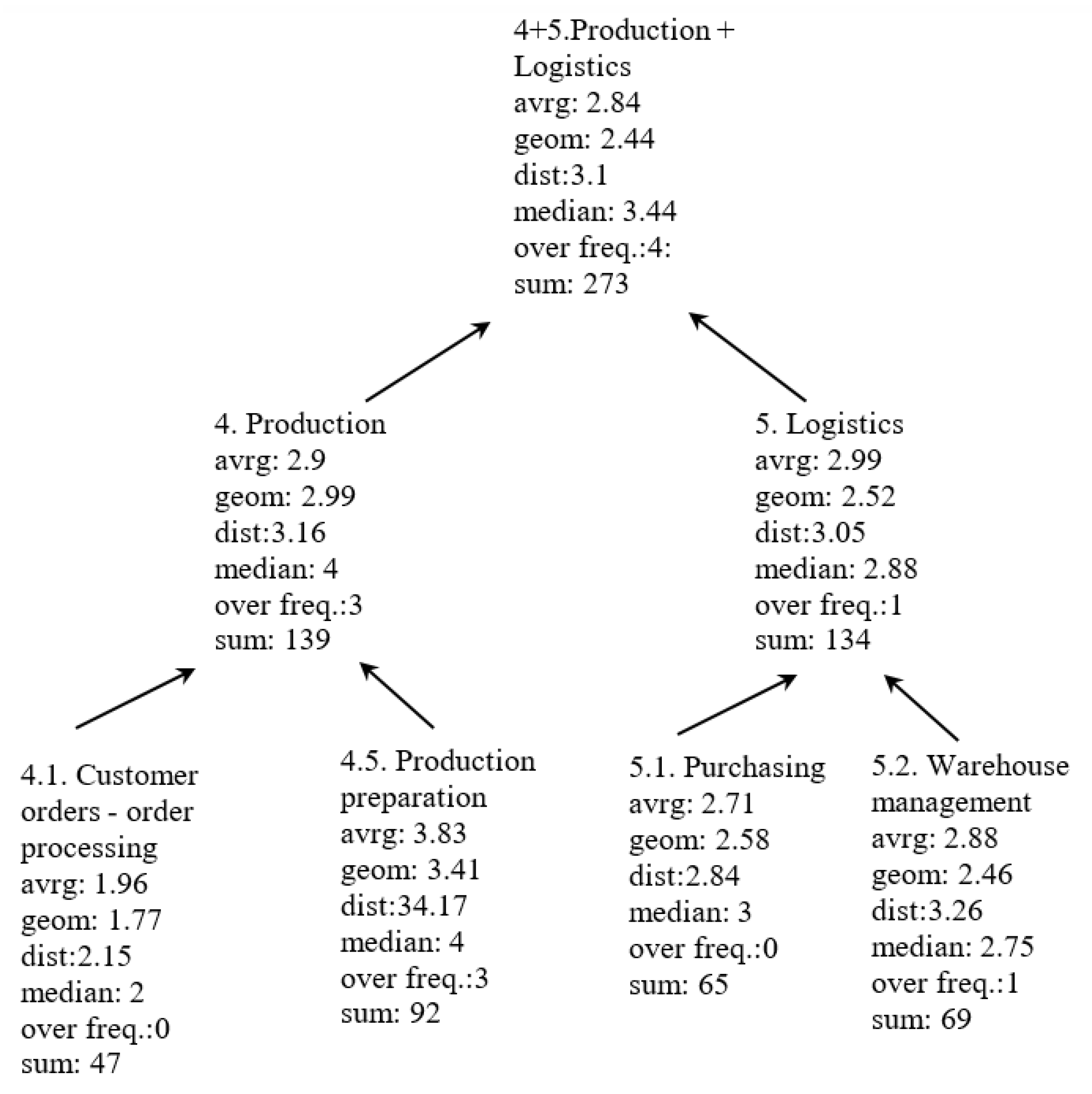
In Figure 1, we connected the corresponding data obtained with different aggregation directions. For example, the arithmetic mean is 1.96–1.96, the geometric mean is 1.86–1.8, and the median is 1.77–1.97. Surprisingly, the two aggregation directions led to nearly identical results. However, this finding cannot be generalized, as it depends on the data. The next level of aggregation is combining production and logistics. The aggregation results along the entire hierarchy are shown in Figure 2.
3.3.2. Aggregating Warnings
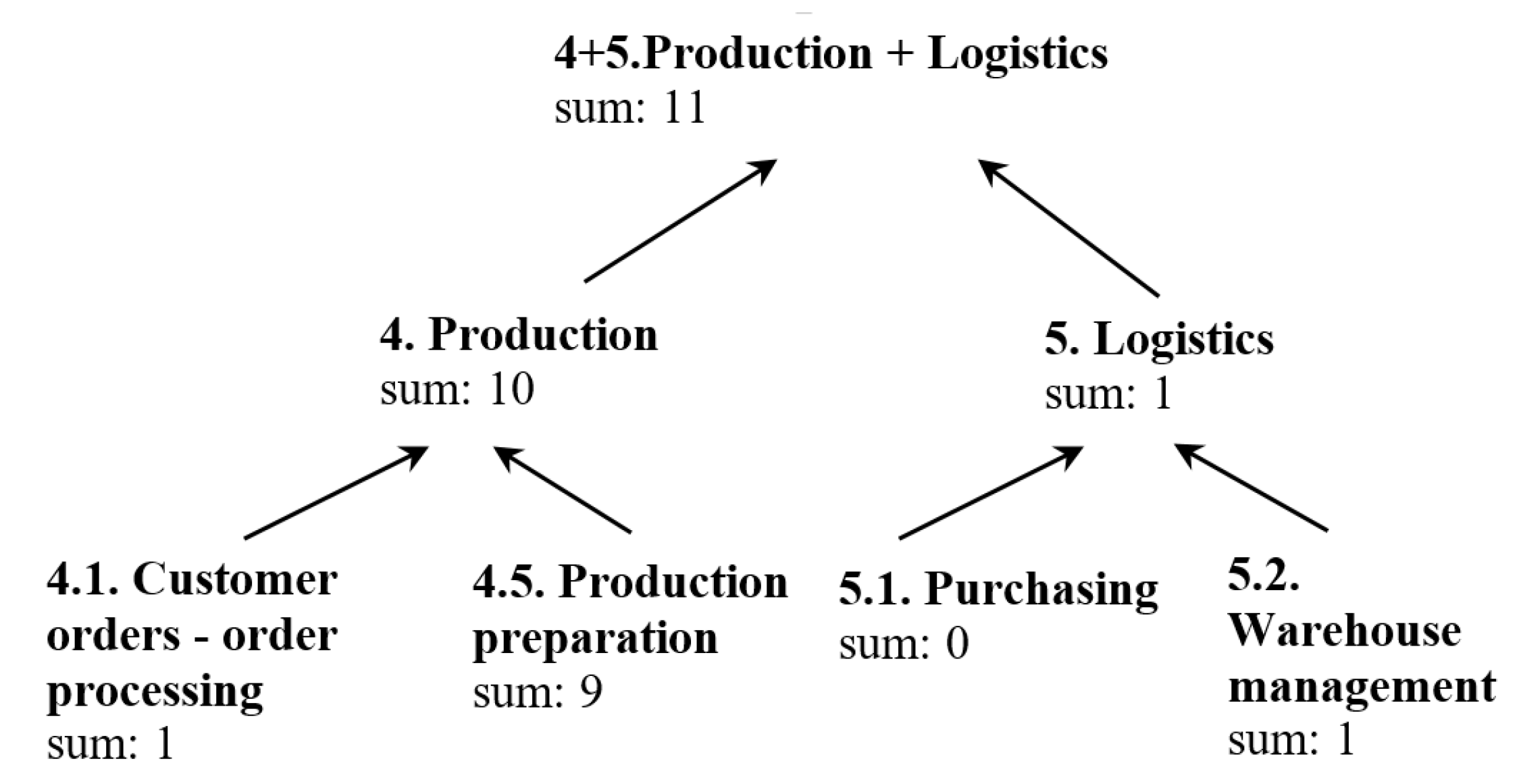
Warnings can also be aggregated. We aggregated the warnings along the hierarchy, as shown in Figure 3.
The function results can be summarized as follows:
One issue with the product function is apparent: strong bias. As a result, warnings may result in Type I or Type II errors. Normalization of the product to the interval [1/10, 10] is not a good solution because this distortion remains. Although 10, as the largest scale value, is psychologically advantageous for judging the risk, in practice, small aggregated risk values are generated, even if there are only a few small values among the component risks. This result can be observed in the prod/10 lines in Figure 1. These low values lead to cumulative bias during further aggregations. Thus, for expected value-type aggregated risk values or heterogeneous components, we recommend the geometric mean or potentially the radial distance as opposed to the product. As a result of the above findings, horizontal aggregation is proposed for the lowest level, while vertical aggregation is proposed for higher levels. As it can be seen in the Figure 2 and Figure 3, the multi-level aggregation can be implemented with risk values and warnings as well. Combining this with the two-way (horizontal and vertical) aggregation directions offers a versatile, multipurpose application opportunity that cannot be found in the literature. A further option to use this hierarchical structure is to generate risk mitigation countermeasures.
3.3.3. Generating Preventive Actions
Following the four steps of the proposed method (Section 2.1.2), first, the aggregated risk values were calculated by using the six risk components and the failure modes in the lowest evaluation level. Five aggregation methods, namely, (1) the (arithmetic) mean, (2) geometric mean, (3) median, (4) maximum, (5) and product normalized to the interval [1, 10] methods, were used to calculate the values of the rows (process components) and columns (risk components). The processes, subprocesses, and failure modes are highlighted in Figure 4. In addition, the background color of each cell indicates the risk level, with red cells indicating higher risk values and green cells indicating lower risk values.
The aggregated values are calculated in two ways, as shown in Figure 4. The left side of Figure 4 shows the first method, in which the risk values of the process components are aggregated first, whereas the right side of Figure 4 shows the opposite calculation method.
A comparison of the results shown in Figure 4 indicates that the different aggregation methods result in the same trends in the aggregated risk values. This finding was confirmed by the seriation results, in which the process and risk components were calculated at the same level, and the biclustering results, in which the sets of risk and process components were selected simultaneously. Therefore, only the first aggregation mode was considered.
To specify the set of risk/process components that must be mitigated, we use two methods. In the first approach, which is an unsupervised method, a predefined threshold matrix is not necessary. In this case, we want to identify the set of risk/process components and their aggregations that are greater than a specified quantile. In contrast, a threshold matrix is specified in the supervised risk evaluation method, with the risk event matrix specifying the risk values of the risk and process components to be mitigated. However, because the risk and process components have common corrective/preventive tasks, this set should also be collected by seriation and biclustering methods.
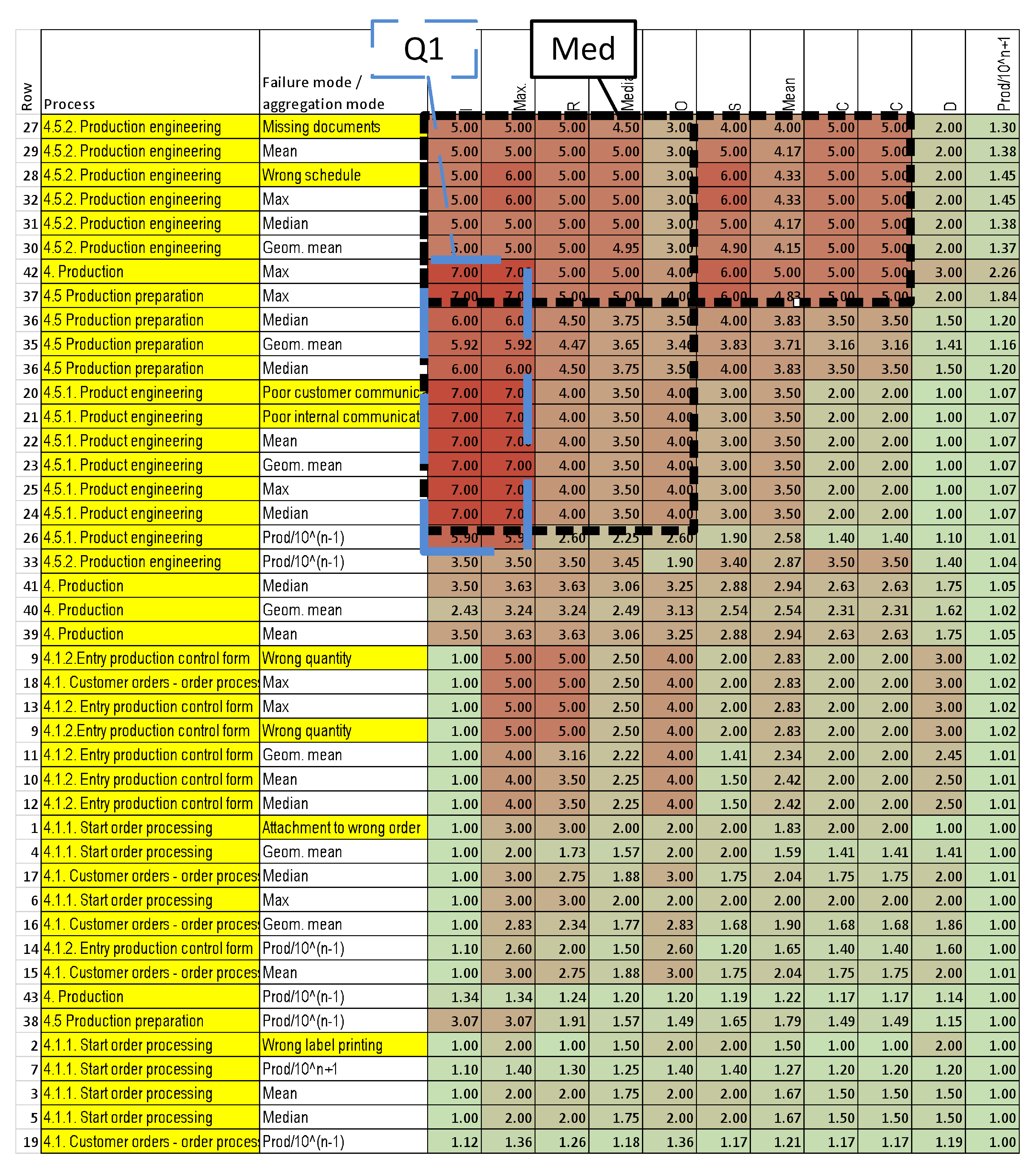
Figure 5 shows the seriation (step 3) and biclustering (step 4) results for two thresholds ( (Med) and (Q1)).
Figure 5 identifies two overlapping (Med) biclusters and one overlapping (Q1) bicluster. Increasing the value of leads to smaller, cleaner biclusters. Because the risk/process components and their aggregations are both considered, the selected and omitted rows and columns must discussed.
The seriation and biclustering results indicate the set of risk and process components and their aggregations. The results show that the risk values in the production preparation process (4.5) and the risk components during the product engineering (4.5.1) and production engineering (4.5.2) processes should both be mitigated. However, the customer orders (4.1) and their subprocesses were not selected. Although both biclusters identified risk component information (I), neither specified the detection (D) value. The maximum aggregation metric, which identifies the riskiest process and risk components, is always applied to the bicluster; however, the production metric, which is used in the FMEA approach, is never applied. The results also show that if there are several risky processes in a higher aggregation level, the mean and median cannot be used to identify the risks to be mitigated.
Figure 6 shows specific thresholds for the risk components and their aggregations. A risk value should be mitigated (red background cells) if its value is greater than or equal to the threshold value. In this example, thresholds are specified for the risk components and their aggregations; however, thresholds are not specified for the process components and their aggregations. Therefore, common thresholds are assumed for all kinds of processes.
Figure 6 shows the seriated and biclustered risk-level matrices for different risk events. In this case, two overlapping biclusters can be specified for both the and parameters that indicate the sets of risk components and their aggregations, as well as the sets of process components and their aggregations. If the risk-level matrix is seriated and biclustered according to the binary values of the risk event matrix, the set of specified risk/process components is similar to the set generated by the unsupervised risk evaluation method (see Figure 5). Additionally, in this case, two overlapping biclusters can be identified. However, the Q1 and Med biclusters are identical. In this case, the purity can be increased by increasing the value of the parameter. Regardless of whether the threshold matrix is included or excluded, the identified risk values that should be mitigated specify the set of corrective/preventive improvement tasks (see Figure 7). Figure 7 shows part of the matrix of corrective/preventive actions. Five tasks, namely, (1) feedback on customer communication, (2) feedback on internal communication, (3) meeting deadlines and faster recognition, (4) more frequent updates, and (5) improving forecasts, are considered in the failure mode level, whereas the maintaining requirements and increasing discipline, training, and bonuses tasks are considered in the aggregated levels. It is important to note that corrective/preventive actions do not need to be specified for all cells. Because the maximal values are corrected if and only if one of the risk/process components must be corrected, corrective/preventive actions should be specified only for the risk/process components.
Figure 7 shows the selected cells for parameters and .
In this practical example, both selections required aggregated corrective/preventive tasks, such as maintaining requirements and increasing discipline, training, and bonuses. This result indicates that not only should failures be corrected or prevented but also that these failures should be prevented at higher risk and process levels.
4. Summary and Conclusions
A real-world example is used to demonstrate the proposed novel multilevel matrix-based risk assessment method for mitigating risk. The paper contributes three key findings to the literature. () The proposed set of multilevel matrices, known as the enterprise-level matrix (ELM), supports the whole risk assessment process, including identifying the risks (e.g., the RLM), evaluating the risks (e.g., the TLM), and determining the corrective/preventive actions for risk mitigation (e.g., the ALM). () The multilevel matrix structure allows decision makers to address the process and risk components and their multipurpose aggregations in the same matrix. As a result, the process components, all levels of the process and risk components, the aggregated risk values and the risk areas in all levels of the enterprise can be evaluated simultaneously. The proposed matrix-based method does not limit the number of risk components or the number of levels in the aggregation hierarchy. In addition, to the best of our knowledge, this is the first method that aggregates both the risk and process components to evaluate risks at different process levels. () By employing seriation and biclustering methods, the risk-level and threshold-level matrices can both be reordered to identify warnings or risks for the process and risk components simultaneously. If more than one aggregation method is employed to aggregate the risk/process components, the employed data mining method, namely, the biclustering and seriation method, selects the appropriate aggregation functions, which indicate the risks in higher process and risk aggregation levels. The employed data-mining method specifies multilevel submatrices that identify the process components, processes, process areas, risk components and risk areas simultaneously. According to the proposed multilevel submatrices, including the RLM and TLM, the appropriate corrective/preventive actions can be proposed based on the ALM matrix to mitigate risks at different levels.
In this work, we ignored the case where there is a dependency between risk components. This is a limitation compared to real cases and opens research opportunities in the future. In the practical example, we omitted the weighting of the risks. However, this limitation can be easily solved by using formulas containing weights. A practical implementation limitation is that the choice between two types of aggregation direction and several functions is a time-consuming process.
Author Contributions
Conceptualization, Z.K.; Methodology, Z.T.K.; Validation, T.C. and I.M.; Writing–original draft, Z.K. and Z.T.K. All authors have read and agreed to the published version of the manuscript.
Funding
This work has been implemented by the TKP2021-NVA-10 project with the support provided by the Ministry of Culture and Innovation of Hungary from the National Research, Development and Innovation Fund, financed under the 2021 Thematic Excellence Programme funding scheme.
Data Availability Statement
Not applicable.
Conflicts of Interest
The authors declare no conflict of interest.
Nomenclature
| AHP | Analytical Hierarchy Process |
| ALM | Action-Level Matrix |
| ANP | Analytical Network Process |
| Criticality factor | |
| Consistency Index | |
| Consistency Ratio | |
| Vector of risk factors | |
| EDAS | Evaluation Based on the Distance from the Average Solution |
| ELECTRE | Elimination and Choice Expressing the Reality |
| ELM | Enterprise-Level Matrix |
| FMEA | Failure Mode and Effects Analysis |
| Fuzzy FMEA | Fuzzy Failure Mode and Effects Analysis |
| GRA | Grey Relational Analysis |
| ISO | International Standardization Organization |
| K | Invention function |
| MULTIMOORA | Multiplicative Form of the Multiobjective Optimization by Ratio Analysis |
| n | Number of risk factors |
| PROMETHEE | Preference Ranking Organization Method for Enrichment Evaluations |
| RAP | Risk Aggregation Protocol |
| Random Consistency Index | |
| RLM | Risk-Level Matrix |
| RPN | Risk Priority Number |
| SRD | Sum of Ranking Differences |
| Threshold vector | |
| TLM | Threshold-Level Matrix |
| TODIM | TOmada de Decisao Iterativa Multicriterio |
| TOPSIS | Technique for Order Preference by Similarity to the Ideal Solution |
| TREF | Total Risk Evaluation Framework |
| Risk aggregation function | |
| VIKOR | VIsekriterijumska optimizacija i KOmpromisno Resenje |
| Vector of weights | |
| Warning rules | |
| WS | Warning System |
References
- Bani-Mustafa, T.; Zeng, Z.; Zio, E.; Vasseur, D. A new framework for multi-hazards risk aggregation. Saf. Sci. 2020, 121, 283–302. [Google Scholar] [CrossRef]
- Bjørnsen, K.; Aven, T. Risk aggregation: What does it really mean? Reliab. Eng. Syst. Saf. 2019, 191, 106524. [Google Scholar] [CrossRef]
- Pedraza, T.; Rodríguez-López, J. Aggregation of L-probabilistic quasi-uniformities. Mathematics 2020, 8, 1980. [Google Scholar] [CrossRef]
- Pedraza, T.; Rodríguez-López, J. New results on the aggregation of norms. Mathematics 2021, 9, 2291. [Google Scholar] [CrossRef]
- Fattahi, R.; Khalilzadeh, M. Risk evaluation using a novel hybrid method based on FMEA, extended MULTIMOORA, and AHP methods under fuzzy environment. Saf. Sci. 2018, 102, 290–300. [Google Scholar] [CrossRef]
- Liu, H.C.; Liu, L.; Liu, N. Risk evaluation approaches in failure mode and effects analysis: A literature review. Expert Syst. Appl. 2013, 40, 828–838. [Google Scholar] [CrossRef]
- Spreafico, C.; Russo, D.; Rizzi, C. A state-of-the-art review of FMEA/FMECA including patents. Comput. Sci. Rev. 2017, 25, 19–28. [Google Scholar] [CrossRef]
- Karasan, A.; Ilbahar, E.; Cebi, S.; Kahraman, C. A new risk assessment approach: Safety and Critical Effect Analysis (SCEA) and its extension with Pythagorean fuzzy sets. Saf. Sci. 2018, 108, 173–187. [Google Scholar] [CrossRef]
- Maheswaran, K.; Loganathan, T. A novel approach for prioritization of failure modes in FMEA using MCDM. Int. J. Eng. Res. Appl. 2013, 3, 733–739. [Google Scholar]
- Ouédraogo, A.; Groso, A.; Meyer, T. Risk analysis in research environment–part II: Weighting lab criticity index using the analytic hierarchy process. Saf. Sci. 2011, 49, 785–793. [Google Scholar] [CrossRef]
- Yousefi, S.; Alizadeh, A.; Hayati, J.; Baghery, M. HSE risk prioritization using robust DEA-FMEA approach with undesirable outputs: A study of automotive parts industry in Iran. Saf. Sci. 2018, 102, 144–158. [Google Scholar] [CrossRef]
- Bognár, F.; Hegedűs, C. Analysis and Consequences on Some Aggregation Functions of PRISM (Partial Risk Map) Risk Assessment Method. Mathematics 2022, 10, 676. [Google Scholar] [CrossRef]
- Kosztyán, Z.T.; Csizmadia, T.; Kovács, Z.; Mihálcz, I. Total risk evaluation framework. Int. J. Qual. Reliab. Manag. 2020, 37, 575–608. [Google Scholar] [CrossRef]
- Wang, J.; Wei, G.; Lu, M. An extended VIKOR method for multiple criteria group decision making with triangular fuzzy neutrosophic numbers. Symmetry 2018, 10, 497. [Google Scholar] [CrossRef]
- Wei, G.; Zhang, N. A multiple criteria hesitant fuzzy decision making with Shapley value-based VIKOR method. J. Intell. Fuzzy Syst. 2014, 26, 1065–1075. [Google Scholar] [CrossRef]
- Kutlu, A.C.; Ekmekçioğlu, M. Fuzzy failure modes and effects analysis by using fuzzy TOPSIS-based fuzzy AHP. Expert Syst. Appl. 2012, 39, 61–67. [Google Scholar] [CrossRef]
- Wei, G.W. Extension of TOPSIS method for 2-tuple linguistic multiple attribute group decision making with incomplete weight information. Knowl. Inf. Syst. 2010, 25, 623–634. [Google Scholar] [CrossRef]
- Chen, N.; Xu, Z. Hesitant fuzzy ELECTRE II approach: A new way to handle multi-criteria decision making problems. Inf. Sci. 2015, 292, 175–197. [Google Scholar] [CrossRef]
- Figueira, J.R.; Greco, S.; Roy, B.; Słowiński, R. An overview of ELECTRE methods and their recent extensions. J. Multi-Criteria Decis. Anal. 2013, 20, 61–85. [Google Scholar] [CrossRef]
- Ghorabaee, M.K.; Zavadskas, E.K.; Amiri, M.; Turskis, Z. Extended EDAS method for fuzzy multi-criteria decision-making: An application to supplier selection. Int. J. Comput. Commun. Control 2016, 11, 358–371. [Google Scholar] [CrossRef]
- Zindani, D.; Maity, S.R.; Bhowmik, S. Fuzzy-EDAS (evaluation based on distance from average solution) for material selection problems. In Advances in Computational Methods in Manufacturing; Springer: Berlin, Germany, 2019; pp. 755–771. [Google Scholar] [CrossRef]
- Liao, H.; Xu, Z. Multi-criteria decision making with intuitionistic fuzzy PROMETHEE. J. Intell. Fuzzy Syst. 2014, 27, 1703–1717. [Google Scholar] [CrossRef]
- Vetschera, R.; De Almeida, A.T. A PROMETHEE-based approach to portfolio selection problems. Comput. Oper. Res. 2012, 39, 1010–1020. [Google Scholar] [CrossRef]
- Li, X.; Wei, G. GRA method for multiple criteria group decision making with incomplete weight information under hesitant fuzzy setting. J. Intell. Fuzzy Syst. 2014, 27, 1095–1105. [Google Scholar] [CrossRef]
- Sun, G.; Guan, X.; Yi, X.; Zhou, Z. Grey relational analysis between hesitant fuzzy sets with applications to pattern recognition. Expert Syst. Appl. 2018, 92, 521–532. [Google Scholar] [CrossRef]
- Liu, H.C.; Fan, X.J.; Li, P.; Chen, Y.Z. Evaluating the risk of failure modes with extended MULTIMOORA method under fuzzy environment. Eng. Appl. Artif. Intell. 2014, 34, 168–177. [Google Scholar] [CrossRef]
- Liu, H.C.; You, J.X.; Lu, C.; Shan, M.M. Application of interval 2-tuple linguistic MULTIMOORA method for health-care waste treatment technology evaluation and selection. Waste Manag. 2014, 34, 2355–2364. [Google Scholar] [CrossRef] [PubMed]
- Huang, Y.H.; Wei, G.W. TODIM method for Pythagorean 2-tuple linguistic multiple attribute decision making. J. Intell. Fuzzy Syst. 2018, 35, 901–915. [Google Scholar] [CrossRef]
- Wang, J.; Wei, G.; Lu, M. TODIM method for multiple attribute group decision making under 2-tuple linguistic neutrosophic environment. Symmetry 2018, 10, 486. [Google Scholar] [CrossRef]
- Héberger, K. Sum of ranking differences compares methods or models fairly. TrAC Trends Anal. Chem. 2010, 29, 101–109. [Google Scholar] [CrossRef]
- Héberger, K.; Kollár-Hunek, K. Sum of ranking differences for method discrimination and its validation: Comparison of ranks with random numbers. J. Chemom. 2011, 25, 151–158. [Google Scholar] [CrossRef]
- Gueorguiev, T.; Kokalarov, M.; Sakakushev, B. Recent trends in FMEA methodology. In Proceedings of the 2020 7th International Conference on Energy Efficiency and Agricultural Engineering (EE&AE), Ruse, Bulgaria, 2–14 November 2020; pp. 1–4. [Google Scholar] [CrossRef]
- Filipović, D. Multi-level risk aggregation. ASTIN Bull. J. IAA 2009, 39, 565–575. [Google Scholar] [CrossRef]
- Ayyub, B.M. Risk Analysis in Engineering and Economics; Chapman and Hall/CRC: Boca Raton, FL, USA, 2014; p. 640. [Google Scholar]
- Keskin, G.A.; Özkan, C. An alternative evaluation of FMEA: Fuzzy ART algorithm. Qual. Reliab. Eng. Int. 2008, 25, 647–661. [Google Scholar] [CrossRef]
- AIAG-VDA. Failure Mode and Effects Analysis—FMEA Handbook; Verband der Automobilindustrie, Southfild, Michigan Automotive Industry Action Group: Berlin, Germany, 2019; Volume 1. [Google Scholar]
- Hahsler, M.; Hornik, K.; Buchta, C. Getting Things in Order: An Introduction to the R Package seriation. J. Stat. Softw. 2008, 25, 1–34. [Google Scholar] [CrossRef]
- Bar-Joseph, Z.; Gifford, D.K.; Jaakkola, T.S. Fast optimal leaf ordering for hierarchical clustering. Bioinformatics 2001, 17, S22–S29. [Google Scholar] [CrossRef]
- Gusenleitner, D.; Howe, E.A.; Bentink, S.; Quackenbush, J.; Culhane, A.C. iBBiG: Iterative binary bi-clustering of gene sets. Bioinformatics 2012, 28, 2484–2492. [Google Scholar] [CrossRef] [PubMed]
- Kosztyán, Z.T.; Pribojszki-Németh, A.; Szalkai, I. Hybrid multimode resource-constrained maintenance project scheduling problem. Oper. Res. Perspect. 2019, 6, 100129. [Google Scholar] [CrossRef]
- Calvo, T.; Kolesárová, A.; Komorníková, M.; Mesiar, R. Aggregation Operators: Properties, Classes and Construction Methods. In Aggregation Operators; Physica-Verlag HD: Heidelberg, Germany, 2002; pp. 3–104. [Google Scholar] [CrossRef]
- Beliakov, G.; Pradera, A.; Calvo, T. Aggregation Functions: A Guide for Practitioners; Springer-Verlag GmbH: Berlin, Germany, 2008. [Google Scholar]
- Kolesarova, A.; Mesiar, R. On linear and quadratic constructions of aggregation functions. Fuzzy Sets Syst. 2015, 268, 1–14. [Google Scholar] [CrossRef]
- Grabisch, M.; Marichal, J.L.; Mesiar, R.; Pap, E. Aggregation Functions; Cambridge University Press: Cambridge, UK, 2009; Volume 127. [Google Scholar]
- Grabisch, M.; Marichal, J.L.; Mesiar, R.; Pap, E. Aggregation functions: Means. Inf. Sci. 2011, 181, 1–22. [Google Scholar] [CrossRef] [Green Version]
- Marichal, J.L.; Mesiar, R. Meaningful aggregation functions mapping ordinal scales into an ordinal scale: A state of the art. Aequationes Math. 2009, 77, 207–236. [Google Scholar] [CrossRef]
- Zotteri, G.; Kalchschmidt, M.; Caniato, F. The impact of aggregation level on forecasting performance. Int. J. Prod. Econ. 2005, 93, 479–491. [Google Scholar] [CrossRef]
- Malekitabar, H.; Ardeshir, A.; Sebt, M.H.; Stouffs, R.; Teo, E.A.L. On the calculus of risk in construction projects: Contradictory theories and a rationalized approach. Saf. Sci. 2018, 101, 72–85. [Google Scholar] [CrossRef]
Figure 1.
Results of bidirectional aggregation at the lowest level.

Figure 2.
Results of multilevel aggregation.

Figure 3.
Results of multilevel warning aggregation.

Figure 4.
Risk-level matrix for production processes.

Figure 5.
The unsupervised risk evaluation results. The seriated and biclustered risk-level matrices with (Med) and (Q1) are shown.
Figure 5.
The unsupervised risk evaluation results. The seriated and biclustered risk-level matrices with (Med) and (Q1) are shown.

Figure 6.
The supervised risk evaluation results. The seriated and biclustered risk-level matrices for different risk events are shown.
Figure 6.
The supervised risk evaluation results. The seriated and biclustered risk-level matrices for different risk events are shown.

Figure 7.
The matrix of corrective/preventive actions for and .


Table 1.
The structure of a risk-level matrix.
| Risk-Level Matrix | Aspects | ||||||||
|---|---|---|---|---|---|---|---|---|---|
| = Quality | = Environment | ||||||||
| Risk Components | Aggr. | Risk Components | Aggr. | ||||||
| Process | Process | ||||||||
| Components | |||||||||
| Aggregated values | |||||||||
| Process | |||||||||
| Components | |||||||||
| Aggregated values | |||||||||
Table 2.
Characterization of risk aggregation functions.
| Aggregation Function | Advantages | Disadvantages |
|---|---|---|
| Sum | Easy to calculate and relatively good linearity. | Fits additive components only. The resulting scale is not identical to the scale of the components ([1, 10]), which can be an advantage in determining the total risk. The result is a sum rather than an average, and the resulting value is greater than the components’ risks when there are more areas or processes. This characteristic is critical for managing the risks of several or a few areas in managerial work. |
| Arithmetic mean | Easy to calculate and relatively good linearity. The resulting scale is identical to the components’ scale ([1, 10]). | Fits additive components only. The components must be measured on the same interval scale. This function does not return the full risk; for example, it does not take into account the need to manage the risks of several or a few areas. |
| Product | Fits with multiplicative models, such as the expected values of the probability (occurrence) and severity. This is the most commonly used aggregation method | Poor linearity. Does not map to the original [1, 10] scale and instead maps to the interval [1, 10]. |
| Product/10 | Correction to the product function. The resulting scale ([1/10, 10]) is close to the original scale (e.g., [1, 10]). | Poor linearity; mapping to almost the same scale does not help. This function tends to output extremely small values. |
| Geometric mean | Normalizes values in different ranges; thus, various scale intervals can be applied. The resulting scale is identical to the components’ scale ([1, 10]). | Not easy to calculate in practice. This function fits better with multiplicative models than with other models. |
| Radial distance / | Moderately good linearity when compared to the linearity of other functions. | The calculation is not easy in practice. |
| Median | The resulting scale is the same as the components’ scale, and this function can also be used on ordinal scales. | The calculation is not easy in practice. The scale is relatively rough and can be considered correct only for homogeneous risk components. |
| Maximum | Easy to calculate. The large values focus attention on critical areas. | Poor representation of the total risk population. |
| Minimum | Easy to calculate. | Poor representation of the total risk population. |
| Number of values over threshold | Easy to calculate. This method focuses attention on critical areas. | Poor representation of the total risk population. |
| Range and standard deviation | Easy to calculate. These approaches show the range or dispersion of the risk components. | Does not output the risk level. |
| Quantile | Outputs the top occurrence values | Does not output the risk level. |
Table 3.
Examination plan.
| No. | Aggregation Situation | Number of Components | Function | Remark |
|---|---|---|---|---|
| 1 | Aggregation of different risk components of the same entity (process or product component) at the lowest level. (The horizontal aggregation is shown in Table 2, 1a.). | Number of risk components: 6, namely, the occurrence, severity, detection, control, information, and range. | Arithmetic mean, corrected product, geometric mean, radial distance, median, minimum, maximum, range, number of values over warning threshold, and sum. | This is the most commonly used aggregation method for calculating the RPN of the components of a product or process. This approach shows the overall risk of a subprocess or product component. |
| 2 | Aggregation of the same risk components of different entities (process or product component) at the lowest level. (The vertical aggregation is shown in Table 2, 2a.). | Number of entities (subprocesses or product components): 1–4. | Same as in 1. | This method shows the overall risk in specific levels. |
| 3 | Further (vertical) aggregation of 1a (1b). | The aggregated values from 1, namely, the number of entities (subprocesses or product components) | Sum, arithmetic mean, and number of values over threshold. | This method shows the total risk in a certain level (within the limitations of the applied function). |
| 4 | Further (horizontal) aggregation of 2a (2b). | The aggregated values from 2; thus, there are 6 risk components, namely, the occurrence, severity, detection, control, information, and range. | Sum, arithmetic mean, and number of values over threshold. | This method shows the total risk in a certain level (within the limitations of the applied function). |
| 5 | Aggregation of all risk components at higher levels (Figure 1 and Figure 2). | Number of risk components: 6; number of entities (subprocesses or product components): 1–4.: | Arithmetic mean, geometric mean, radial distance, median, number of values over warning threshold, and sum | This method shows the total risk in a certain level (within the limitations of the applied function). |
| 5 | Aggregation of warnings (Figure 3). | Number of entities. | Sum and number of values over threshold | This method shows the total risk in a certain level (within the limitations of the applied function). |
| 6 | Generating preventive actions (Figure 4). | Number of entities. | Arithmetic mean, geometric mean, median, maximum, and corr. product | This step selects the threshold for the optimal preventive action. |
Publisher’s Note: MDPI stays neutral with regard to jurisdictional claims in published maps and institutional affiliations. |
© 2022 by the authors. Licensee MDPI, Basel, Switzerland. This article is an open access article distributed under the terms and conditions of the Creative Commons Attribution (CC BY) license (https://creativecommons.org/licenses/by/4.0/).
Share and Cite
MDPI and ACS Style
Kovács, Z.; Csizmadia, T.; Mihálcz, I.; Kosztyán, Z.T. Multipurpose Aggregation in Risk Assessment. Mathematics 2022, 10, 3166. https://0-doi-org.brum.beds.ac.uk/10.3390/math10173166
AMA Style
Kovács Z, Csizmadia T, Mihálcz I, Kosztyán ZT. Multipurpose Aggregation in Risk Assessment. Mathematics. 2022; 10(17):3166. https://0-doi-org.brum.beds.ac.uk/10.3390/math10173166
Chicago/Turabian StyleKovács, Zoltán, Tibor Csizmadia, István Mihálcz, and Zsolt T. Kosztyán. 2022. "Multipurpose Aggregation in Risk Assessment" Mathematics 10, no. 17: 3166. https://0-doi-org.brum.beds.ac.uk/10.3390/math10173166
Note that from the first issue of 2016, this journal uses article numbers instead of page numbers. See further details here.