A Study of Learning Issues in Feedforward Neural Networks

Abstract

When training a feedforward stochastic gradient descendent trained neural network, there is a possibility of not learning a batch of patterns correctly that causes the network to fail in the predictions in the areas adjacent to those patterns. This problem has usually been resolved by directly adding more complexity to the network, normally by increasing the number of learning layers, which means it will be heavier to run on the workstation. In this paper, the properties and the effect of the patterns on the network are analysed and two main reasons why the patterns are not learned correctly are distinguished: the disappearance of the Jacobian gradient on the processing layers of the network and the opposite direction of the gradient of those patterns. A simplified experiment has been carried out on a simple neural network and the errors appearing during and after training have been monitored. Taking into account the data obtained, the initial hypothesis of causes seems to be correct. Finally, some corrections to the network are proposed with the aim of solving those training issues and to be able to offer a sufficiently correct prediction, in order to increase the complexity of the network as little as possible.

1. Introduction: Feedforward Networks and Their Gradient Descendent Based Training Algorithm

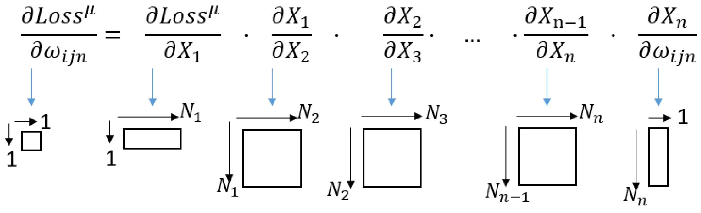
Feedforward networks are a kind of deep neural network (DNN) that process the input through a certain number of processing layers, one of the most common being the multi-layer perceptron. For this reason, the authors of the current work have studied this architecture and the stochastic gradient descendent (SGD) based training algorithms. A widely used process to train any kind of DNN is the supervised learning process. In this process, a set of training data inputs from the current DNN is labelled with the correct answer the network predicts; the training process consists of passing each of the inputs, called patterns, through the net and measuring the difference between the expected output and the real one. The function that measures this difference is known as the Loss function and there are different functions that can be applied for it. Once the Loss on the current pattern has been obtained, it is back propagated from the output of the DNN to the input, correcting the weights of the different Layers in the net accordingly. There are different methods to back propagate this Loss into the synaptic weights of the layers; the one taken as the study objective for the current article is the SGD method, which is widely used and adapted to different necessities by different authors [1,2,3,4,5,6,7,8]. Its objective is to find the minimum of the Loss function by correcting the synaptic weight of the network layers pattern by pattern. To do so, the partial derivative of the current Loss, with reference to the current modifying layer, is applied. The process can be represented as a series of partial derivatives, starting from that of the Loss according to the output layer of the DNN and subsequently multiplying the partial derivative of the layers according to their previous partner until the current modifying layer is reached,

$$\begin{gathered} {\frac{\partial Loss}{\partial X_n}}_{1x{N}_n}={\frac{\partial Loss}{\partial X_1}}_{1x{N}_1}.{\left({\displaystyle \prod }_{i=1}^{n-1}\frac{\partial X_i}{\partial X_{i+1}}\right)}_{N_{1}x{N}_n} \\ {\frac{\partial Loss}{\partial W_n}}_{N_{n}x{N}_{n+1}}={\left(\frac{\partial Loss}{\partial X_n}\right)}_{N_{n}x1}^T{\left(\frac{\partial X_n}{\partial W_n}\right)}_{1x{N}_{n+1}}^T \\ {\frac{\partial X_n}{\partial W_n}}_{N_{n+1}x1}={\left(X_{n+1}^{\mu }\right)}_{N_{n+1}x1} \end{gathered}$$

(1)

where µ is the current pattern, Wn is the synaptic weights matrix of the current layer n, X_n is the current layer and the output layer is considered as the layer “1”. The dimensions of each of the matrices and vectors are attached as sub-indices of them. N_n is the number of output connections of the nth layer and µ represents the fact that the associated element is related to the current pattern being analysed.

As applying the direct result of the derivative to the synaptic weights can be very unstable, a learning ratio α is applied to it, whose value is defined inside (0, 1]. Additionally, an inertia momentum β is added to the learning equation, allowing the learning process to aim for the Loss function absolute minimum value, instead of being trapped in a local minimum that can result in training which is not efficient enough. Otherwise, the wrong perception of a more complex network needs to be designed to solve the current problem [9,10,11]; this parameter is also defined inside (0, 1]. After these two considerations are taken into account, the learning equation is as follows:

$$\nabla W_n=-\alpha \left(\frac{\partial Loss}{\partial W_n}\right)+\beta M_n^t; M_n^{\left(t+1\right)}=M_n^t+\nabla W_n$$

(2)

where $M_n^t$ is the momentum matrix of the current learning step that will be updated in each of the learning steps. The over-parametrisation of a neuronal network makes it insufficiently flexible to correctly predict inputs outside the training bundle. This appears after having trained the network over several epochs, thus enabling it to achieve a low training error. However, with the test data, the error prediction obtained by the network is high and continues to grow along with the number of training epochs. To avoid this, there are some techniques that can be applied. The first is called Batch or Mini-Batch [12,13] and, as its name implies, it splits the training patterns bundle into a number of smaller batches. They are then passed through the DNN, calculated, the Loss function is averaged out of them and the network is trained through this Loss function averaging. This method, depending on the batch size chosen, can not only reduce the computational time needed for an epoch of training network, but also affect the performance results of the network itself. Another possible method is Dropout [12,13,14]; here, in the process of learning a pattern, or a batch of them, some of randomly chosen synaptic weights in the current layer are not going to suffer any modification, only partially learning the pattern and thus making the network learn in a more generalist way, avoiding having to learn the finest details of the pattern. Finally, for this study case, randomizing the pattern order for entering the DNN learning process is also contemplated. Thus, by avoiding learning with a fixed, predetermined order of patterns, this overtraining can be avoided and corrected, as the network does not learn any kind of order logic from the input patterns, and this can be unprofitable for the final prediction results.

The rest of the paper is organised as follows: in Section 2, the background of the neural network analysis is shown, including what other authors have done to solve the different training algorithm problems; in Section 3, the issues that have been found in the SGD algorithm by this paper’s authors and the possible solutions proposals for them are set out; in Section 4, the experiments performed are displayed; in Section 5, the possible future works are commented and in Section 6, the conclusion obtained after executing them.

2. Background

The training of a neural network is known to be focused on fitting the weights of the input neurons in order to achieve a response in the output layer that corresponds to the known data. It is recognised that neural networks with high accuracy and good performance tend to have very complex internal structures. As analysed by Congjie et al. [15], attempting to over-interpret neural networks will make the performance of the model worse. In this way, the main problems that arise in neural networks are defined. On the one hand, it is necessary to quantify the interpretability and accuracy of the established rules, so that it also becomes necessary to extract these rules from the model. On the other hand, there is the need to make these rules more balanced between a good interpretability and accuracy, these being opposite objectives.

With this objective in mind, different network training techniques have been proposed, with the need for optimisation. The most common training method is back propagation (BP). As far as optimisation is concerned, Particle Swarm Optimisation (PSO) tends to be used. Gudise et al. [16] present a study of the computational requirements; it is shown that, for the learning of non-linear feedforward network functions, the weights converge earlier with the use of PSO. In addition, it also shows how the use of PSO requires fewer computations to obtain the same error, defining this optimisation better for fast learning. In the case of linear function applications, Zhang [11] discusses the use of momentum algorithms in neural networks, thus obtaining sufficient and necessary conditions for convergence in stationary iterations. Furthermore, regardless of the application, it is necessary to investigate the effect of the neural network, the activation functions and the number of neurons needed in the hidden layers for learning, as performed by Sari [17].

Using the exploration speed of the PSO, studies present hybrid algorithms. Coupling it with the Cuckoo search (CS), which has a good ability to find the global optimum with slow convergence, avoids a premature convergence while also tracing the whole space (Jeng-Fung et al. [18]). To avoid excessive training time in complex neural networks, studies such as Manjula Devi et al. [19] present a type of training called fast linear adaptive skipping training (LAST), where only the input samples that do not categorise perfectly in the initial epochs are screened, without affecting the accuracy. The increase in data parallelism with the development of the hardware must also be taken into account. This increase also has a negative effect on the training time, which is measured by the ‘number of steps needed to obtain the out-of-sample error goal’, as Shallue et al. [20] show in their article. Other authors, such as Xiong Cheng et al. [21] and Long Viet Ho et al. [22], have studied the possibility of using predatory algorithms in combination with feedforward neural networks to try to optimise the process of adjusting the different network parameters, without falling into local minimum error scenarios; this optimises the network, while still being sufficiently generalist and flexible. Divya Bairathi et al. [23] and Stefan Milosevic et al. [24] propose using a swarm like algorithm for this purpose.

Overtraining can also impair the performance of neural networks. As Erkaymaz [25] has proved, feedforward Newman-Watts small-world artificial neural networks show better classification and prediction results compared to conventional feedforward networks. Thus, they propose a resilient feedforward Newman–Watts small-world artificial neural network that assumes repaired topological initial conditions. This reduces overfitting without increasing the complexity of the algorithm. It should be noted that neural network training often involves two phases. On the one hand, there is an unsupervised pre-training to learn the parameters of the neural network. On the other hand, there is a supervised fine-tuning, which improves on what was learned in the previous phase. This is what Wani et al. [14] do in their study, performing the second phase with a standard BP algorithm. In their work, they propose a new point of view that integrates the parameters gained based on BP and a dropout technique for evaluation and fine tuning, thus improving performance.

Unlabelled data in an inference problem can sometimes cause the underlying distribution to be adversely perturbed. To solve this, Najafi et al. [26] propose unifying two main learning approaches, namely semi-supervised learning (SSL) and distributional robust learning (DRL). In this way, they are able to quantify the role of unlabelled data in generalisations based on general conditions. The lack of labelling is a loss of values. Choudhury et al. [27] suggest a mechanism to use these unlabelled data to design classifiers, a different technique than predicting them, using an auto-encoder neural network with two training scenarios. By means of the neighbour rule, the initial values are at first obtained with the auto-encoder, and then refined by minimising the error.

In order to optimise the loss function, a widely used resource is the SGD during training, with the aim of optimisation. This method has the disadvantage of falling into a local optimum very easily, getting rid of the gradient problems that need to be solved. Authors such as Lai et al. [2] present a hybrid algorithm that takes into account this problem by combining the advantages of the Lclose PSO algorithm and the SGD. The theoretical characteristics of neural networks do not specify data on the loss of information in gradients that do not propagate. They propose an algorithm called memorised sparse back propagation (MSBP) to combat the problem of information loss, storing the non-propagated gradients in a memory and learning these in subsequent times (Zhang et al. [28]). In this way, it is possible to avoid convergence in probability based on specific conditions.

Following another path, Meng et al. [3] have been able to demonstrate that the use of the SGD has the guaranteed convergence for non-convex tasks such as those necessary in deep learning. To do this, they present a mathematical formulation for the procedure of processing practical data in distributed machine learning, called global/local shuffling. As for the computational time when the number of neurons is high, the computational time itself is also high, when training algorithms for recurrent neural networks based on gradient error. These networks are unstable in the search for the minimum. Authors such as Blanco et al. [29] propose the use of real coded genetic algorithms that use the appropriate operators for coding.

An adaptive method for optimisation, formulated to equip gradient-based updating with adaptive scaling in a sophisticated way, is the ADAM method, presented by Kobayashi [7]. They propose a new optimiser that integrates both concepts, implicitly carrying on the adaptive scaling of the statistical uncertainty of the gradients.

The use of the SGD has the disadvantage of generating a delay in the updating of the weight of the neurons. To solve this, some authors propose taking this delay into account in the SGD algorithm, so that its impact is minimised. The guided stochastic gradient descendent (gSGD) directs convergence by comparing the deviation that cannot be predicted, caused by delays (Sharma [5]). Other authors, such as Wang et al. [6], propose an algorithmic approach to verify the communication and calculation of neural networks, thus accelerating the training process. They add an anchor model to each node, thus ensuring convergence in cases of non-convex objective functions. It also ensures a reduction of the total runtime.

In addition to the gradient function of neural networks, it is possible to take into account their Jacobian. It is known that, when the number of parameters of the layers tends to infinity, this becomes a Gaussian process where a quantitatively predictive description is possible. Doshi et al. [30] demonstrate a new method for diagnosis. To do this, they induced the partial Jacobians of the neural network, defined as the derivatives of pre-activations. Recurrence relationships are used for Jacobians, using them for criticality analysis. Wilamowski et al. [31] have created a new algorithm with neuron-by-neuron computing methods, focusing on the gradient vector and the Jacobian matrix. They show that Jacobian computation requires second-order algorithms, and they have a computation complexity similar to that of the first-order gradient learning methods.

3. Training Algorithms: Issues, Analysis and Possible Solutions

The problem comes when one of the patterns is not correctly learned, making the network fail in its predictions on similar patterns; the training of a neural network is a very time-consuming process and missing out on learning a certain pattern and being forced to try to make a new training bundle, or add additional epochs of learning, can be unaffordable. Several authors have tried different solutions to this problem [1,2,28,32].

∇Wn in Equation (2) is a gradient matrix associated to the nth layer’s synaptic weights when the μth pattern is exposed to the neural network. Usually, this matrix changes for different pattern data. Therefore, there is a difference between the ∇Wn matrix and its mean value throughout the mini batch data. Two main issues are detected in the learning process:

The first learning issue comes when a certain pattern µ has a partial derivative of the Loss function related to a certain synaptic weight $\omega$ijn, in opposition to the average value for all-over patterns in the training batch; $\omega$ijn, is the ith row and jth column element in Wn, with n being a certain layer in the DNN.

$$\mathrm{sign}\left(\frac{\partial Los{s}^{\mu }}{\partial {\omega }_{ijn}}\right)\ne sign\left(\frac{\partial Loss}{\partial {\omega }_{ijn}}\right)$$

(3)

where $\frac{\partial Loss}{\partial {\omega }_{ijn}}$ is the synaptic weight’s mean value calculated for all the patterns in the batch.

In this case, the pattern presented is offering a completely different sense of correction for the net compared to the rest of the patterns. So, neural networks must choose between improving certain data when the Loss function is high or improving the average Loss function for all the data in the mini batch. This kind of problem is usually linked to the neural network architecture more than to the learning algorithm. The second learning issue is due to the partial derivative of the Loss function of the current pattern µ for a certain weight ij in a certain layer n when it reaches a value of 0,

$$\frac{\partial Los{s}^{\mu }}{\partial {\omega }_{ijn}}=0$$

(4)

In this case, the back propagated Loss function has reached a point where its values are negligible or a rectified linear unit (ReLU) operation has made its values, as the forward signal has a negative value. In any case, this effect means that the synaptic weights of the layers before the current one will not be updated correctly, as there would be no more updates on the subsequent layers, which would depend on that weight; this effect is known as the vanishing of the back propagated signal.

3.1. Gradient Vanishing Issue

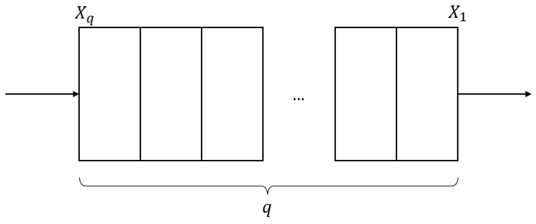
The analysis to be performed in this section is related to the Jacobian values of the different layers that form a DNN. They are the ones to be studied in the context of this article, so as to explain the different issues found in the training process of the neural network. A generic case study is presented in Figure 1. It indicates a structure of a number q of layers of a neural network, each layer associated to a synaptic weight ${\omega }_{ijn}$, where n is the current layer position in the [1, q] set. In this case, X_q refers to the input layer and X₁ to the output layer.

It is recognised that the synaptic weight of each layer can be calculated with Equation (5), where ${\omega }_{ijn}$ represents the synaptic weight of ith row and jth column on the layer n, t refers to the current step of the learning process, α to the learning ratio, and $\frac{\partial Los{s}^{\mu }}{\partial {\omega }_{ijn}}$ is the derivative of the loss function in relation to the pattern µ. X_n vector is the activation vector of the nth layer. The ${\omega }_{ijn}$ weight only has effect on ith component. So, the partial derivation of the activation vector has all null components except the ith component. This component, is equal to jth component of (n + 1)th activation vector. The momentum is avoided in the Equation (5) for simplicity.

$${\omega }_{ijn}\left(t+1\right)={\omega }_{ijn}\left(t\right)-\alpha \frac{\partial Los{s}^{\mu }}{\partial {\omega }_{ijn}}$$

(5)

The relationship between the function $\partial Los{s}^{\mu }$ and $\partial {\omega }_{ijn}$, shown in Equation (6), is also defined.

$$\frac{\partial Los{s}^{\mu }}{\partial {\omega }_{ijn}}=\frac{\partial Los{s}^{\mu }}{\partial X_1}·\frac{\partial X_1}{\partial X_2}·\frac{\partial X_2}{\partial X_3}·\dots ·\frac{\partial X_{n-1}}{\partial X_n}·\frac{\partial X_n}{\partial {\omega }_{ijn}}$$

(6)

In this way, the Jacobians to be analysed are defined generically. A study can, therefore, be developed concerning the size of each component of the previous equation, as represented in Figure 2; as it is known that the equation is made up of vectors and matrices, N_n marks the number of output connections the n layer has.

With this knowledge, the way in which the modulus fades out will be analysed. If the rank of any of the Jacobian matrix components of Equation (6) is zero or very low, the information is lost and the modulus will vanish, because the kernel dimensions of these Jacobian matrices are very high. If the dimensions of the kernel space of one Jacobian matrix are high, many vectors would have the null vector as their image. So, the error actualization is lost in such a matrix. Therefore, if in any of the Jacobians’ rank is null or very low, there will be a loss of signal between the (n − 1)th and nth layers. Thus, if $\Vert \frac{\partial Los{s}^{\mu }}{\partial X_n}\Vert$ is zero, then the error is null. In this case, the training algorithm has achieved the objective for the training pattern concerned. Finally, the last righthand term, $\frac{\partial X_n}{\partial {\omega }_{ijn}}$ is a column vector. All the components of this vector are null, except for ith component of the vector, which contains the jth activation of the nth layer. If the value of $\Vert \frac{\partial X_n}{\partial {\omega }_{ijn}}\Vert$ is null, the vanishing of error actualization occurs between the 1st and nth layers. In any case, if $\frac{\partial X_n}{\partial {\omega }_{ijn}}$ is composed mainly of 0 values and few elements with remarkable information, that layer could be a candidate for pruning in a future state of the training process [33]. This, however, is an aspect to be analysed in future works.

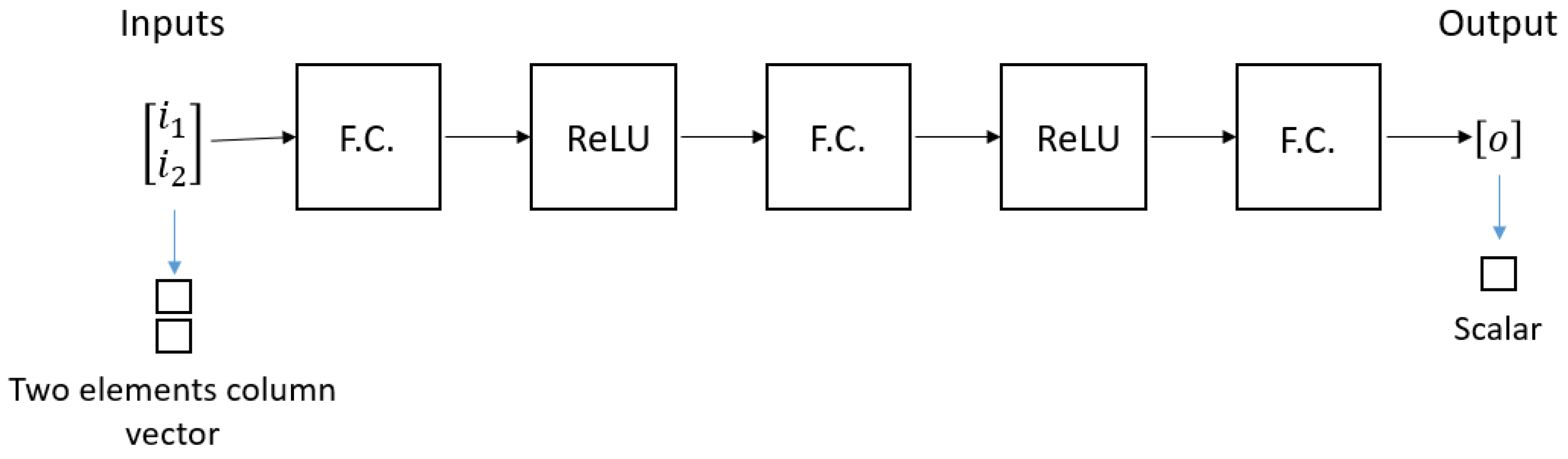
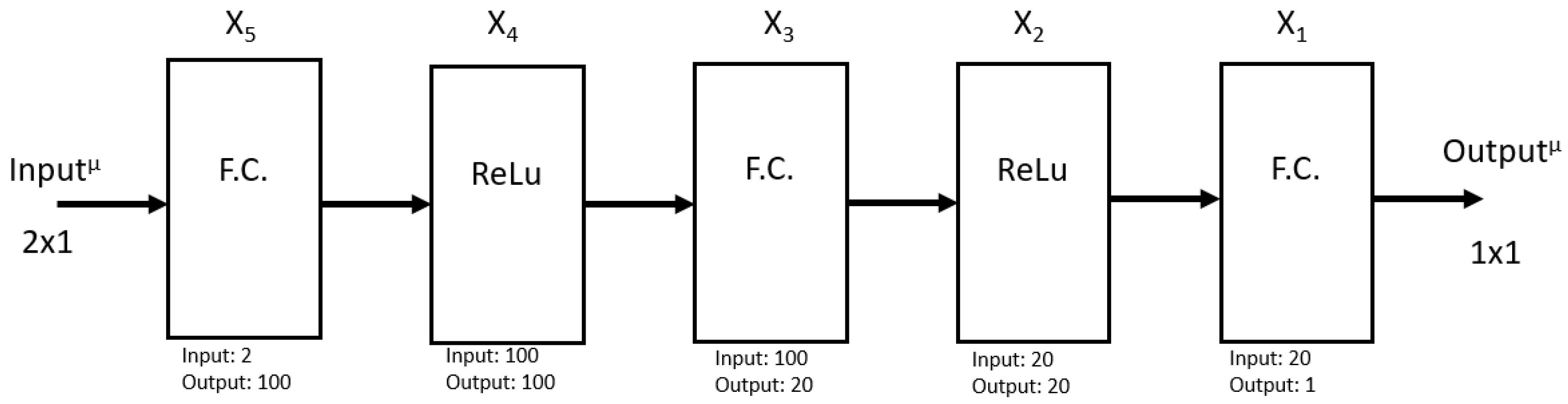
In the particular case of this study, a neural network with the structure of Figure 3 is analysed. It can be noted that there are two inputs in the form of a column vector and a unique output, which is a scalar. The network is composed of three fully connected layers, annotated as FC and two ReLU activation functions.

Continuing with the criteria analysed in Equation (6) and considering there will be 3 layers to be analysed, the following case studies are considered.

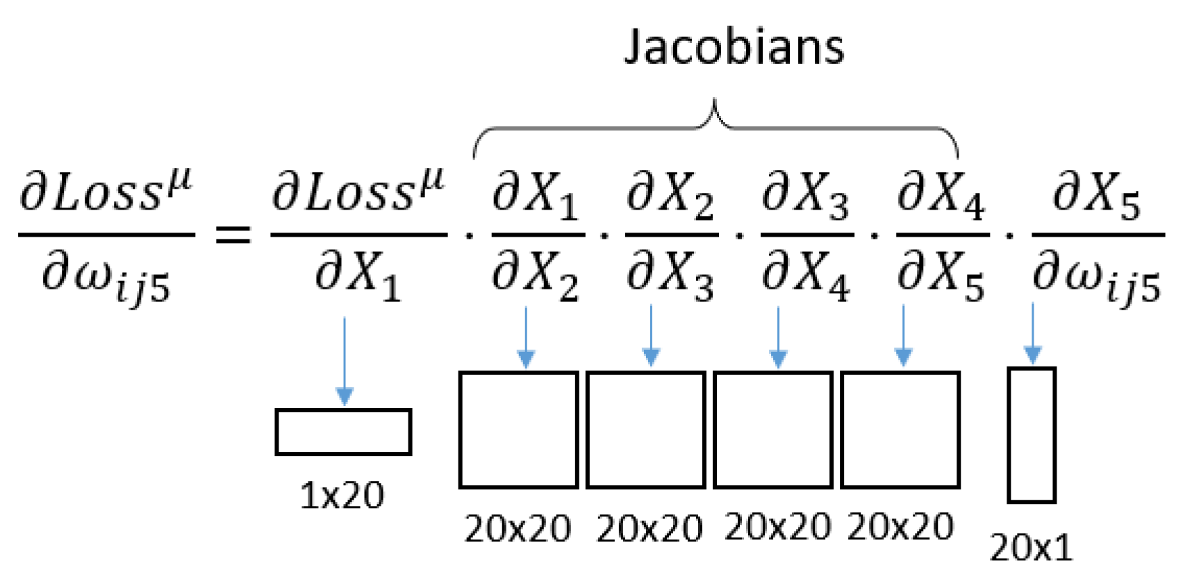
• On the one hand, in the case of taking the network structure as a whole, Equation (6) is reformulated as shown in Equation (7).

$$\frac{\partial Los{s}^{\mu }}{\partial {\omega }_{ij5}}=\frac{\partial Los{s}^{\mu }}{\partial X_1}·\frac{\partial X_1}{\partial X_2}·\frac{\partial X_2}{\partial X_3}·\frac{\partial X_3}{\partial X_4}·\frac{\partial X_4}{\partial X_5}·\frac{\partial X_5}{\partial {\omega }_{ij5}}$$

(7)

In this case, there are four Jacobian matrices to be analysed, with the sizes shown in Figure 4.

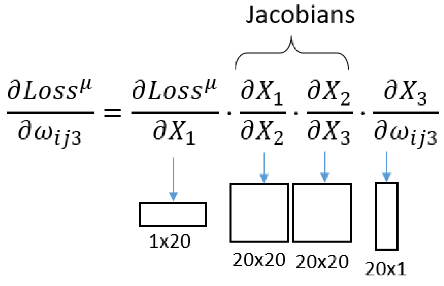
• On the other hand, it can be analysed starting from the third layer, in which case the Jacobians of Equation (8) are posed.

$$\frac{\partial Los{s}^{\mu }}{\partial {\omega }_{ij3}}=\frac{\partial Los{s}^{\mu }}{\partial X_1}·\frac{\partial X_1}{\partial X_2}·\frac{\partial X_2}{\partial X_3}·\frac{\partial X_3}{\partial {\omega }_{ij3}}$$

(8)

For this equation, the size of the components is represented in Figure 5.

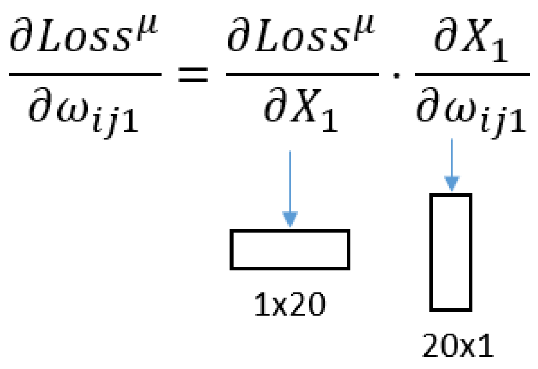
• Finally, the study starting from the output layer is the simplest, since there are no Jacobian matrices, as shown in Equation (9).

$$\frac{\partial Los{s}^{\mu }}{\partial {\omega }_{ij1}}=\frac{\partial Los{s}^{\mu }}{\partial X_1}·\frac{\partial X_1}{\partial {\omega }_{ij1}}$$

(9)

As there are no Jacobians, the equation is only composed of vectors, as shown in Figure 6.

3.2. Opposite Gradient Direction

As said in Section 3.2, one of the possible problems that can occur during the SGD training is the appearance of an opposite direction on the learning vector of a certain pattern µ; so the average learning vector causes the pattern not only to be badly learnt by the network, but also that, in order to learn that pattern, the network will lose information from other patterns in the network. To check this direction divergence, each of the learning matrices $\frac{\partial Los{s}^{\mu }}{\partial W_n}$ formed for a certain bunch of learning patterns have been taken and they have been turned into a vector by coupling all the rows of the matrix into a single one, one after the other. Then, their scalar product has been used and the average value of the entire learning patterns bunch has produced learning matrices. Thus, a φ angle is calculated using the following formula:

$$\cos \left(\phi \right)=\frac{\frac{\partial Los{s}^{\mu }}{\partial W_n}·\frac{\partial Loss}{\partial W_n}}{\left|\frac{\partial Los{s}^{\mu }}{\partial W_n}\right|\left|\frac{\partial Loss}{\partial W_n}\right|},$$

(10)

There are mainly three possible situations that can occur: the cosine value is positive and near to 1, the cosine value is near to 0 and the cosine is negative and near to −1. In the first case, the pattern follows the tendency marked by the average value, and it is being learnt by the network without disturbing the information of other patterns already stored in the net. In the second, the information of the current pattern cannot be correctly learnt on that layer. When the cosine of the rest of the layers also shows this cosine value, the pattern and the nearby patterns will not generate a correct answer, even more so if the cosine is negative. The training process of this pattern will cause the loss of information from other patterns. In the third case, the pattern is in the opposite direction to their average, so the pattern learning will require a severe loss of information from other patterns. When the module value of $\frac{\partial Los{s}^{\mu }}{\partial {\omega }_{ijn}}$ is much bigger than the average $\frac{\partial Loss}{\partial {\omega }_{ijn}}$, the influence on the learning process will be important. There will be cases of patterns correctly learnt by the network, but after analysing their $\frac{{\partial }_{Los{s}^{\mu }}}{\partial {\omega }_{ijn}}$ vectors, they show a big module value with an opposite sign cosine. In this case, those patterns are taken as a “bully” for the current network, since they require the loss of information from other patterns in the current architecture in order to be learnt correctly.

3.3. Training Algorithm Issues, Solutions for Each One

In both cases, the authors propose possible modifications of the network that could contribute to reducing the negative effects of both problems caused for the performance of the network.

3.3.1. Gradient Vanishing Issue

In the case of the gradient vanishing issue, the proposal to correct it would be to include a residual element of the input layer in the following one, thus avoiding the reduced rank of processing layers having such a large effect on the data and also allowing the pattern data to reach a deeper layer. Another possible solution for this issue is the Batch Normalisation process proposed by Ioffe and Szegedy [34] to ensure higher learning rates and reduce the effects of the initial hyper-parametrisation. This technique has been used by other authors [35,36,37,38] to work in the same terms.

3.3.2. Opposite Gradient Direction

In the case of the opposite gradient direction, a possible solution would be to increase the number of connections on the FC layers or to increase the number of FC layers in the network, so it can absorb more aspects of the patterns. As in the gradient vanishing issue, it could also be possible to solve them by pulling residual data forward from the input, thus causing them to be affected by the output layers of the network.

4. Shallow Neural Network Example: Non-Linear Regression of the Mexican Hat Function

A simple example is defined to try to express the different types of mistraining that can happen on a feedforward neural network. The network is composed of five layers, three FC and 2 processing layers, intercalated in a sequence of FC-P-FC-P-FC. The activation functions are ReLU in both cases. The network accepts input arrays of two floating-point elements and generates a scalar floating-point element as output. The Loss function is defined as the Mean Square Error, one of the most usual for this kind of network, which makes a regression out of some data. In Figure 7, it is possible to see the basic architecture of the network.

The training batch is formed by 6241 patterns and 3136 validation patterns to check the correct training of the network and avoid over-training. The function to be learnt by the network is the following:

$$z=sinc\left(x^2+y^2\right) ; x,y\in \left[-0.95, 1\right],$$

(11)

where x and y are the inputs and z is the desired output of the network. The training method is defined as SGD, using no batch training. One hundred epochs of training have been defined, the input data batch being shuffled to prevent any misunderstandings in the learning caused by the relationship of the data because of its specific order, where α and β are set at 0.01 as the typical values of the feedforward training.

During the last epoch of training, assuming that it is the step where minor changes would occur, only the worst learnt pattern would give a significant change to the synaptic weights of the FC layers. After the last training session, the patterns are again passed through the network, classifying them according to the error obtained by comparing the real output with the expected output. With these data, two different groups are made, one having the 20 patterns with the worst performance and the other the 20 with the best performance.

The data taken during the training are the Jacobian values of each layer of the network for each of the patterns, as well as the modification triggered by that pattern and the $\frac{\partial Los{s}^{\mu }}{\partial X_1}$ of that pattern. With these data, the average value of the different $\frac{\partial Loss}{\partial X_n}$ is calculated and, via the scalar product, the angle between the average value and that of the specific patterns is obtained, as well as the relationship between their modules. As stated above, the more perpendicular this angle between the arrays is, the harder it will be to learn that pattern for the network. If it gets to be obtuse or directly opposed, learning that pattern will cause the loss of information from other patterns.

To create the DNN MATLAB 2021a and a library of our own creation are used. In this way, a deeper analysis of the process that takes place in the training of the network can be performed, in order to be able to take the necessary actions concerning it.

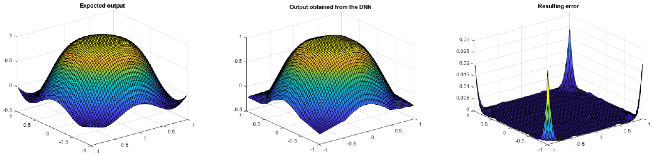
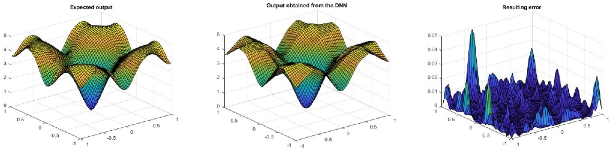
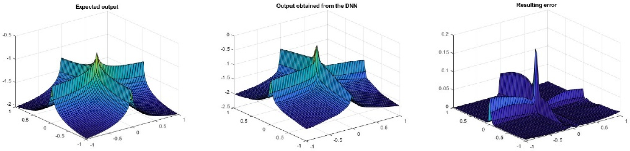
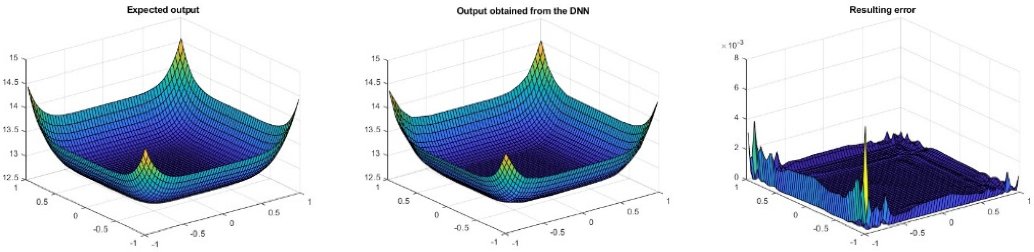
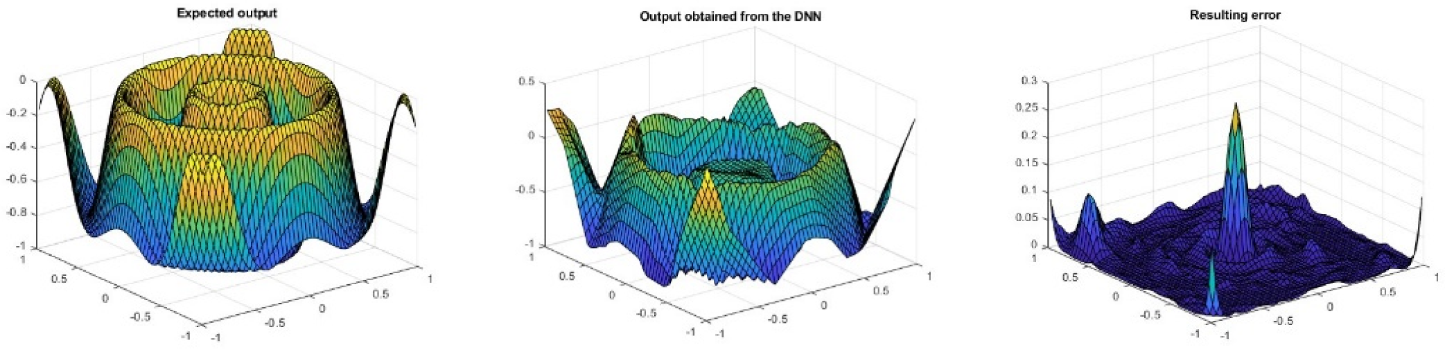
Figure 8 shows, from left to right, the target output of the network, the obtained results and the error between them after the training process described above. As can be seen, the error on the edges of the figure is greater than in the central zone.

After training, having chosen the lists of the best learnt and worst learnt patterns and calculated the average $\frac{\partial Loss}{\partial X_n}$ for every layer,

Table 1. The pattern with the largest output error (x = −0.950, y = −0.950), showing the cosine between the partial derivate of the Loss to the working layer in the average case and the particular pattern case and the relationship between their modules.

Pattern [−0.950; −0.950]	cos(φ)	$\left|\frac{\partial \mathit{L}\mathit{o}\mathit{s}{\mathit{s}}^{\mathit{\mu }}}{\partial {\mathit{X}}_{\mathit{n}}}\right|/\left|\frac{\partial \mathit{L}\mathit{o}\mathit{s}\mathit{s}}{\partial {\mathit{X}}_{\mathit{n}}}\right|$
$\frac{\partial Los{s}^{\mu }}{\partial X_1}$	−1.00	4667.86
$\frac{\partial Los{s}^{\mu }}{\partial X_2}$	−1.00	4668.63
$\frac{\partial Los{s}^{\mu }}{\partial X_3}$	0.55	186.20
$\frac{\partial Los{s}^{\mu }}{\partial X_4}$	0.67	0.01
$\frac{\partial Los{s}^{\mu }}{\partial X_5}$	0.55	180.21
$\frac{\partial Los{s}^{\mu }}{\partial \mathrm{In}}$	0.75	263.88

shows the pattern that has the greatest error compared to the target, with its cosine values and modules relationship. As can be seen, the output layer and the previous one (X₁ and X₂) present a negative value of the cosine and a high value for the relationship of the modules, which means the pattern will need to lose a large amount of information from other patterns on those layers to be able to learn this particular pattern, as the average of the patterns is pointing in the other direction.

In the best learnt patterns list, there are patterns that are learnt in concordance with the average behaviour of the pattern. However, there are still some that present the opposite direction and have a much bigger module than the average one.

Table 2. The data taken from the best learnt pattern (x = 0.525, and y = −0.425).

Pattern [0.525; −0.425]	cos(φ)	$\left|\frac{\partial \mathit{L}\mathit{o}\mathit{s}{\mathit{s}}^{\mathit{\mu }}}{\partial {\mathit{X}}_{\mathit{n}}}\right|/\left|\frac{\partial \mathit{L}\mathit{o}\mathit{s}\mathit{s}}{\partial {\mathit{X}}_{\mathit{n}}}\right|$
$\frac{\partial Los{s}^{\mu }}{\partial X_1}$	1.00	35.73
$\frac{\partial Los{s}^{\mu }}{\partial X_2}$	1.00	35.73
$\frac{\partial Los{s}^{\mu }}{\partial X_3}$	−0.90	1.76
$\frac{\partial Los{s}^{\mu }}{\partial X_4}$	−0.99	0.00
$\frac{\partial Los{s}^{\mu }}{\partial X_5}$	−0.68	2.72
$\frac{\partial Los{s}^{\mu }}{\partial \mathrm{In}}$	−0.99	8.70

shows the data taken from the best learnt pattern. It can be seen that, even if the output layer has the same the direction as the average, it still has a much bigger module. Even though the intermediate layers have opposite direction, the modules are much smaller than for the case of the worst learn pattern. In one of the cases, the relationship between the modules is even less than 1%.

Generally speaking, there are some conclusions that can be reached. On the one hand, the situation of perpendicularity of the learning might lead us to conclude that the network is not prepared to learn some of the patterns correctly, so actions should be taken to improve that learning. On the other hand, the appearance of the opposite direction and large module differences with the average one, means that, for the current architecture of the network, there are some “bully” patterns that force the network to lose a lot of information from other patterns in order to learn these ones; again, a modification of the network should be performed in those layers where this effect is more evident. The effect can be better seen if $\frac{\partial Loss}{\partial W}$ is used instead to compare the average values and the current pattern µ. In

Table 3. Worst learnt pattern’s $\frac{\partial Loss}{\partial W_n}$ for the FC layers. Both weight matrices, the average and pattern µ, are reshaped to a single row array of values before doing the scalar multiplication; otherwise, a bound of results would be generated for each one of the output values of the current layer. The rest of the Layers, the Processing ones, are not displayed, as they would not be modified during the learning process.

Pattern [−0.950; −0.950]	cos(φ)	$\left|\frac{\partial \mathit{L}\mathit{o}\mathit{s}{\mathit{s}}^{\mathit{\mu }}}{\partial {\mathit{W}}_{\mathit{n}}}\right|/\left|\frac{\partial \mathit{L}\mathit{o}\mathit{s}\mathit{s}}{\partial {\mathit{W}}_{\mathit{n}}}\right|$
$\frac{\partial Los{s}^{\mu }}{\partial W_1}$	−0.17	2976.34
$\frac{\partial Los{s}^{\mu }}{\partial W_3}$	0.32	437.15
$\frac{\partial Los{s}^{\mu }}{\partial W_5}$	0.00	6847.99

and

Table 4. Best learnt pattern’s $\frac{\partial Loss}{\partial W_n}$ for the FC layers. As in the worst learnt pattern, the weight matrices are reshaped into a single row array value before doing the scalar multiplication.

Pattern [0.525; −0.425]	cos(φ)	$\left|\frac{\partial \mathit{L}\mathit{o}\mathit{s}{\mathit{s}}^{\mathit{\mu }}}{\partial {\mathit{W}}_{\mathit{n}}}\right|/\left|\frac{\partial \mathit{L}\mathit{o}\mathit{s}\mathit{s}}{\partial {\mathit{W}}_{\mathit{n}}}\right|$
$\frac{\partial Los{s}^{\mu }}{\partial W_1}$	0.98	46.34
$\frac{\partial Los{s}^{\mu }}{\partial W_3}$	−0.7	1.94
$\frac{\partial Los{s}^{\mu }}{\partial W_5}$	−0.07	51.87

, the worst and best learnt patterns are displayed. In the worst case, it can be seen that, in order to learn the pattern, the output layer, X₁, must greatly modify its values in the opposite direction to the average learnt pattern. The intermediate layer, X₃, is partly aligned with the average, while in the input layer, X₅, the pattern will be barely learnt, as it is totally in the orthogonal direction to the average.

On the best learnt case, see Table 4, the output layer is strongly aligned with the average direction of learning, while it is directly in opposition on the intermediate layer, which means, as said before, that information from other patterns must be discarded to learn this pattern. Finally, on the input layer, it is highly orthogonal and in the opposite direction, which means that the pattern will be barely learnt on this layer and some other pattern information will be erased.

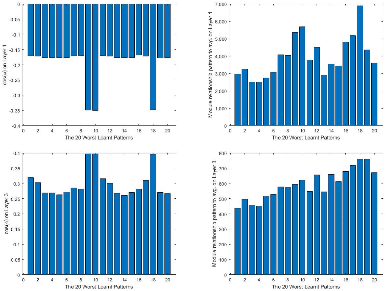
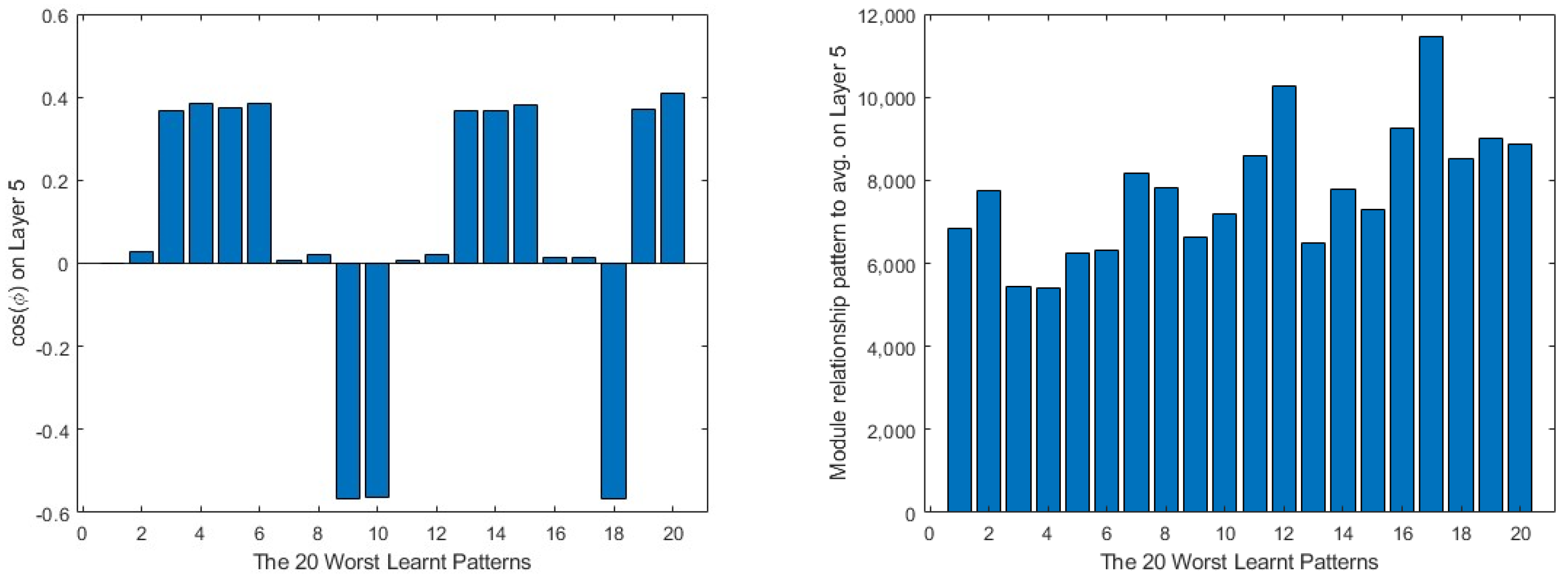
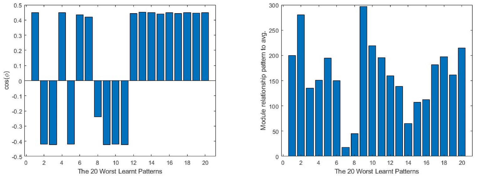
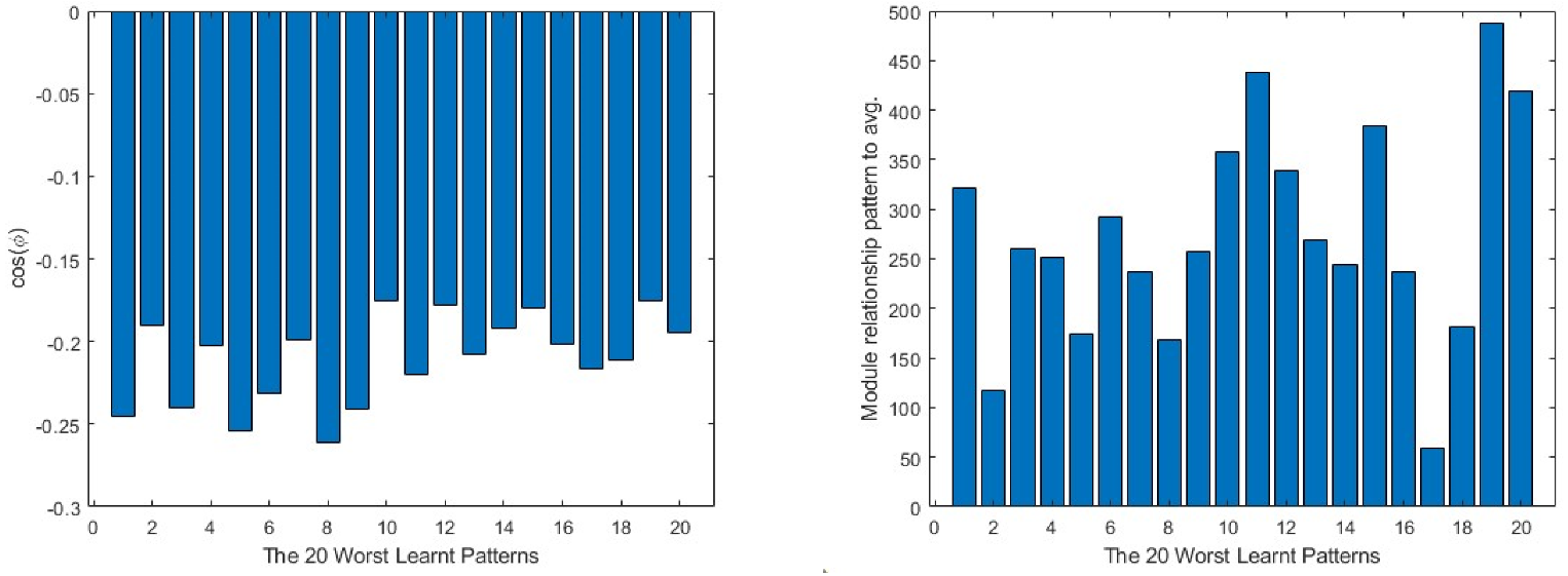
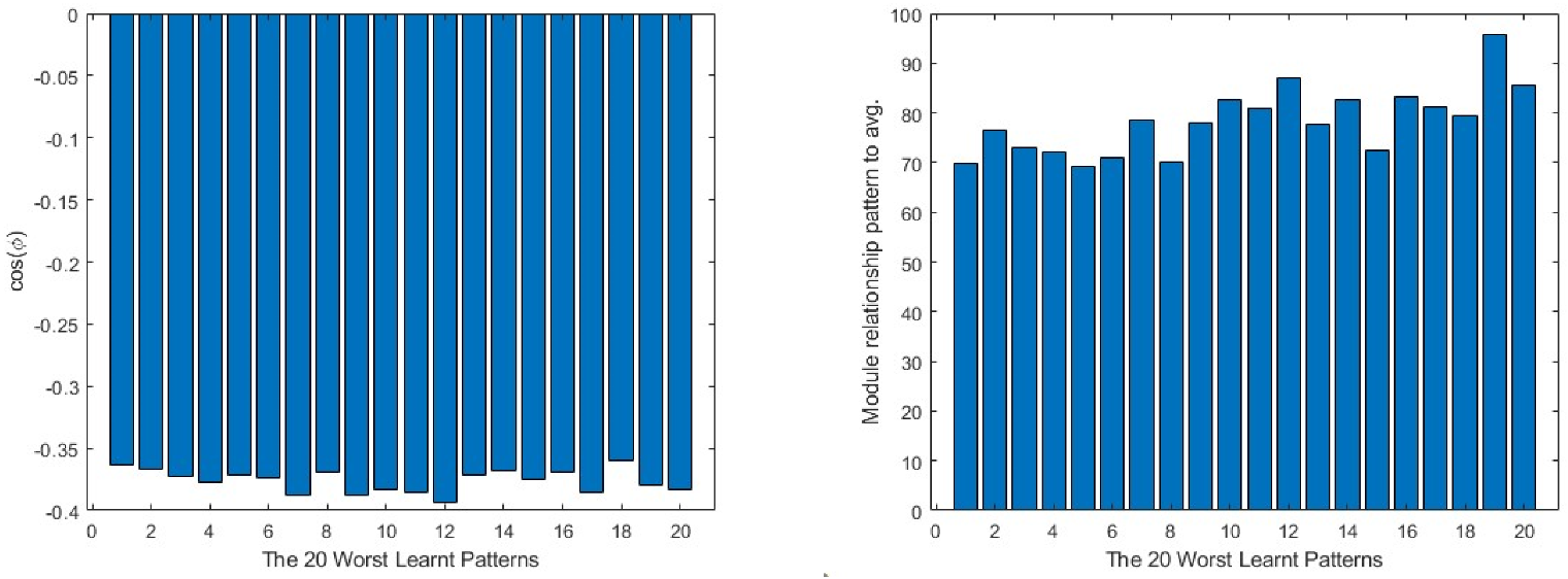
For a more generic view, in Figure 9, taking the 20 worst learnt patterns and looking at their cos(φ) and module relations, it can be seen that the output layer always shows the opposite direction $\frac{\partial Los{s}^{\mu }}{\partial W_n}$ to the average one in all the cases, while in the intermediate layer, it is always partially aligned with it, as the values of the cosine are below the 0.4 value. This means that much of the information concerning the pattern is not being learnt by the layer. The input layer is the one that presents the most random situation, where some of the patterns present a value close to 0 in the cosine and, for the rest, none of them reach a value near 1. Turning to the comparison of the modules, the patterns require a much bigger correction in all the layers than the average produces, the minimum values being over 400 times bigger than the average module.

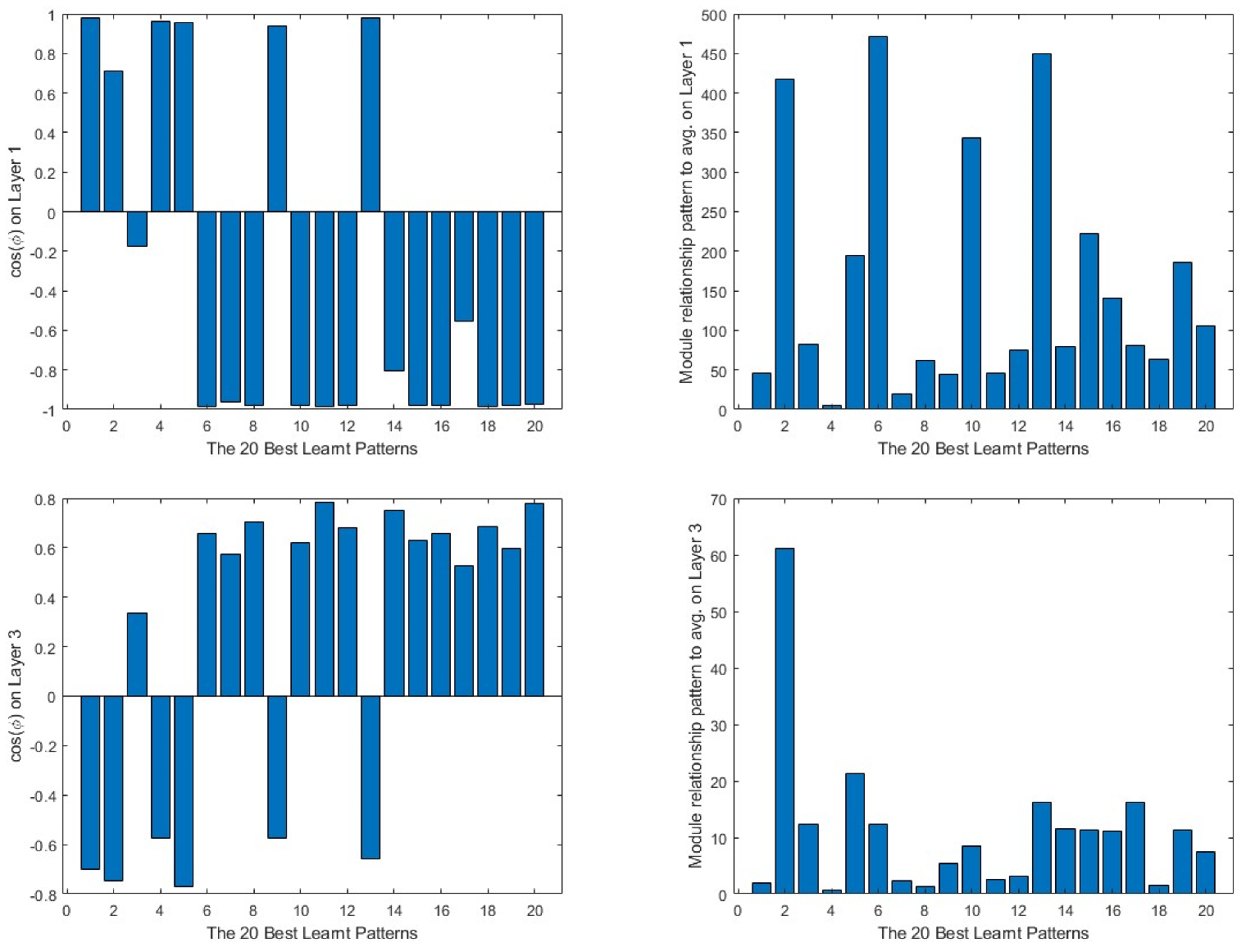
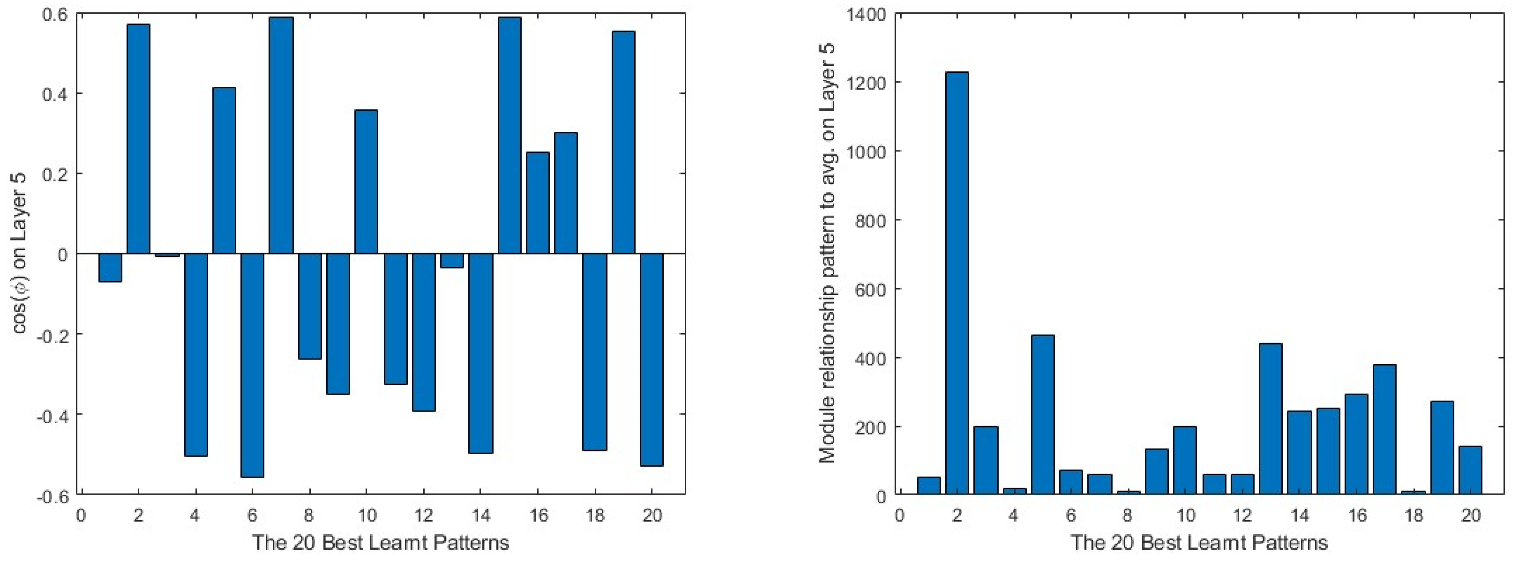
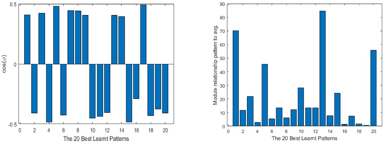
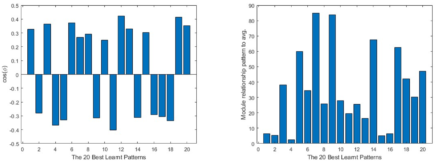
On the other hand, in Figure 10, the same data from the best learnt patterns is shown. As a general view, the absolute value of the cosine is nearer to 1 than in the case of the worst learnt ones. Furthermore, the difference between the modules is much lower in most of the cases. As in the previous group, the input layer presents the less efficient learning parameters.

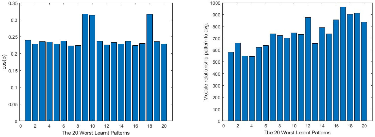
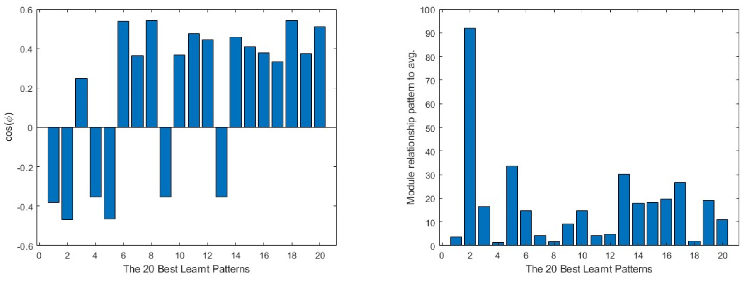
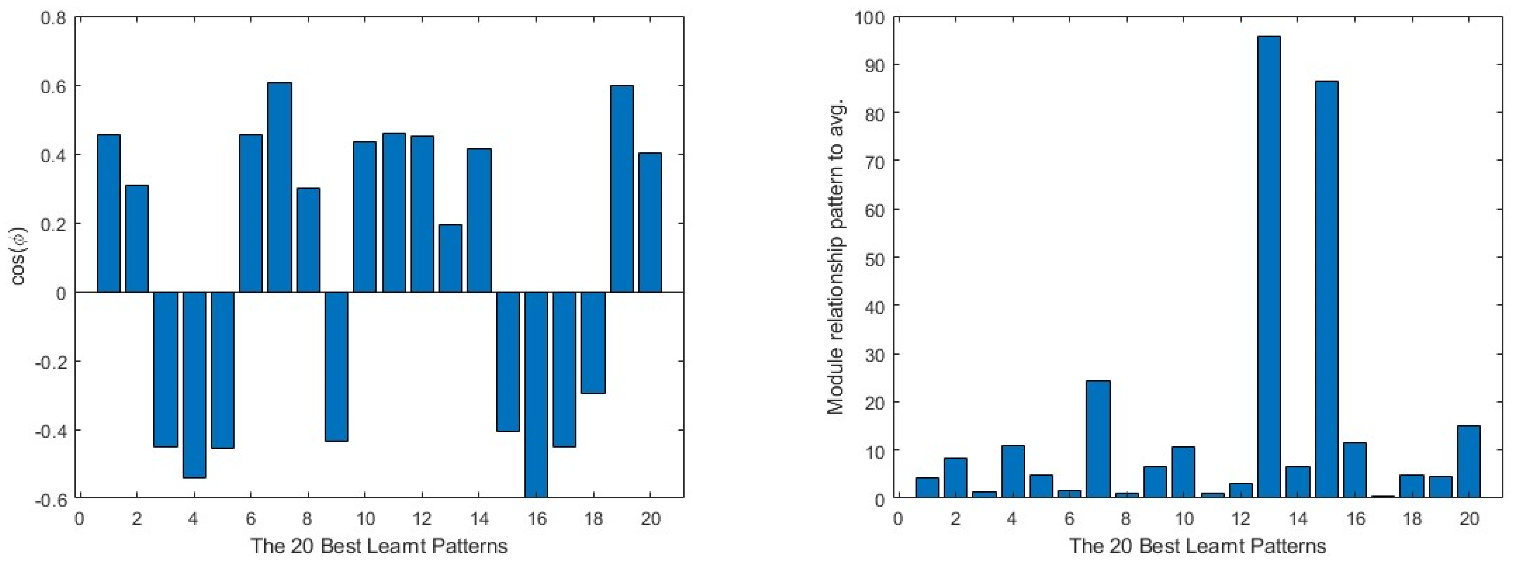
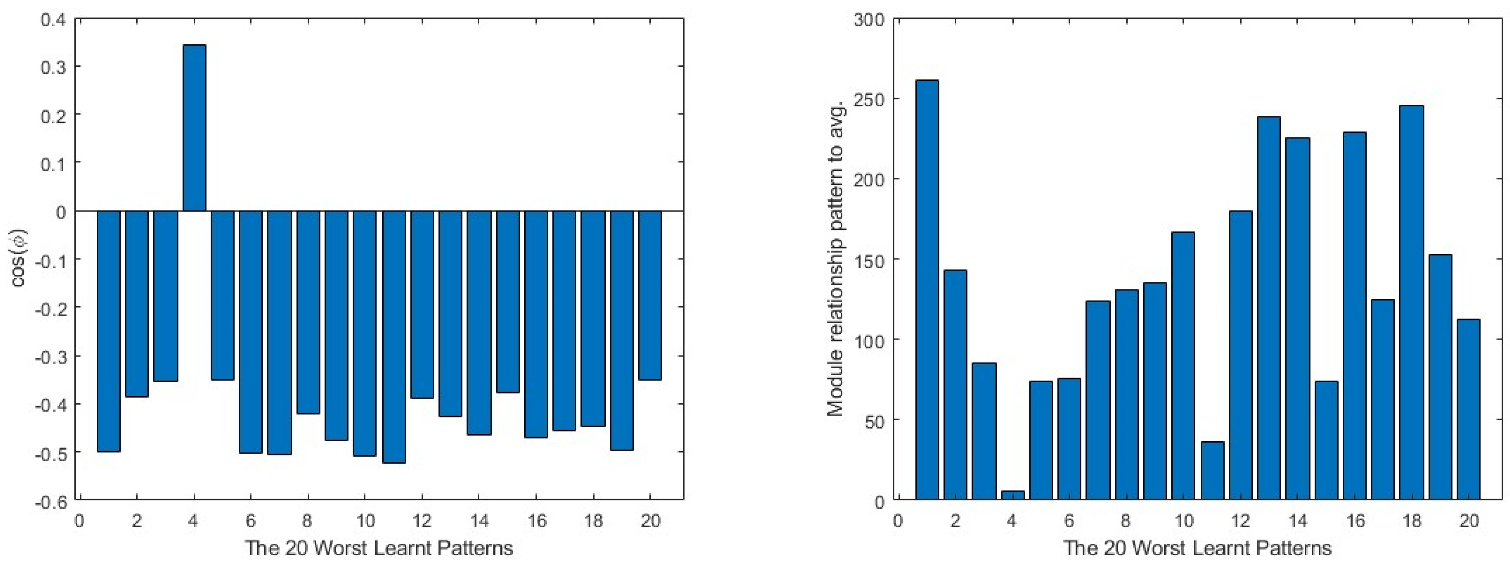
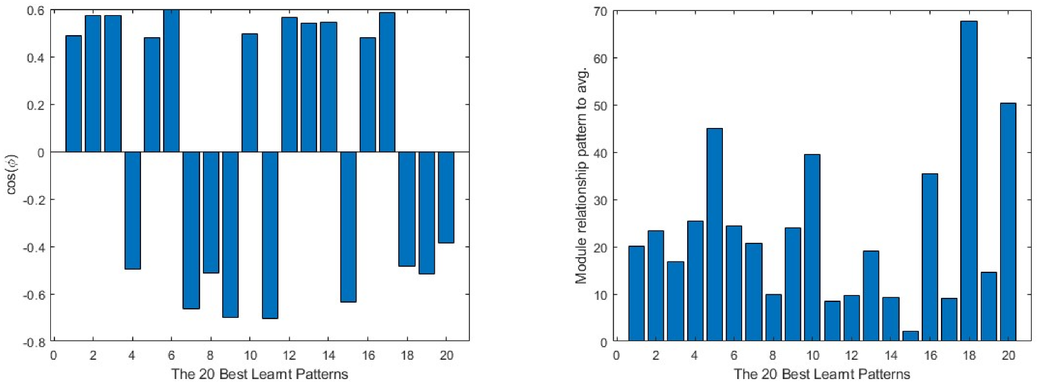
Finally, combining the vectors of these three layers in a single vector, by sequencing them one after the other in a single row vector to analyse the viability of each of the patterns for the current network, it is clear that there are quite big differences between the worst and best learnt patterns. In Figure 11 and Figure 12, the differences in behaviour can be found between these two groups of patterns. The worst learnt patterns are all in the same direction as the average vector, but the cos(φ) value is below 0.4 in all cases, revealing a loss of information in the training process. This can also be seen in the module comparison between the pattern and the average vector, where all the values are over 500; this means that the network needs to change greatly to be able to learn them. On the other hand, the best learnt patterns have a greater variety of direction in the learning process, but it can be considered more closely aligned, as the cos(φ) absolute value is over 0.5 in most cases. On the module side, as they are more easily learnt, the relationship between the modules is less than 50, except in one of the patterns, the second best learnt, which can be classified as a ‘bully’, as it shows a negative cos(φ). What is more, having a high module comparison, this pattern requires the elimination of a large amount of information from other patterns in order to be learnt.

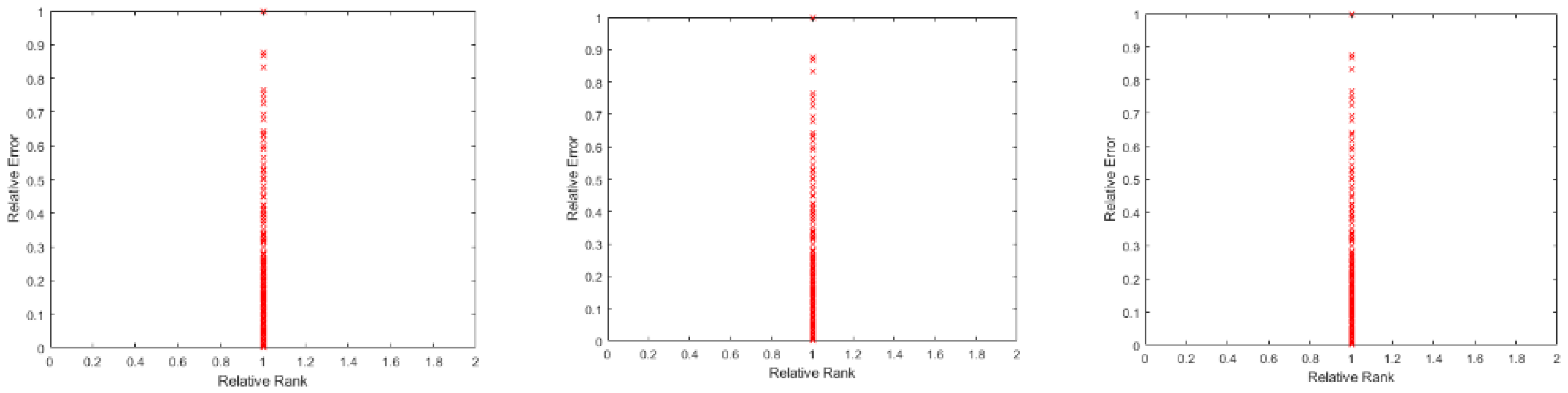
The gradient vanishing side, the different layers’ Jacobians are taken and processed, calculating the rank of each of them and dividing them by their maximum possible rank to obtain a relative rank of each of them, for ease of analysis. The same process was followed with the error of each of the learnt pattern, dividing it by the maximum found error. On the FC layers, the rank is maintained to the maximum in all the patterns, being always the rank equal to the smallest value between the number of inputs and the number of outputs of that layer. On Figure 13, we can see that, on the three layers, the rank of them for all the patterns is always equal to its maximum, which is the smaller number between its inputs and outputs.

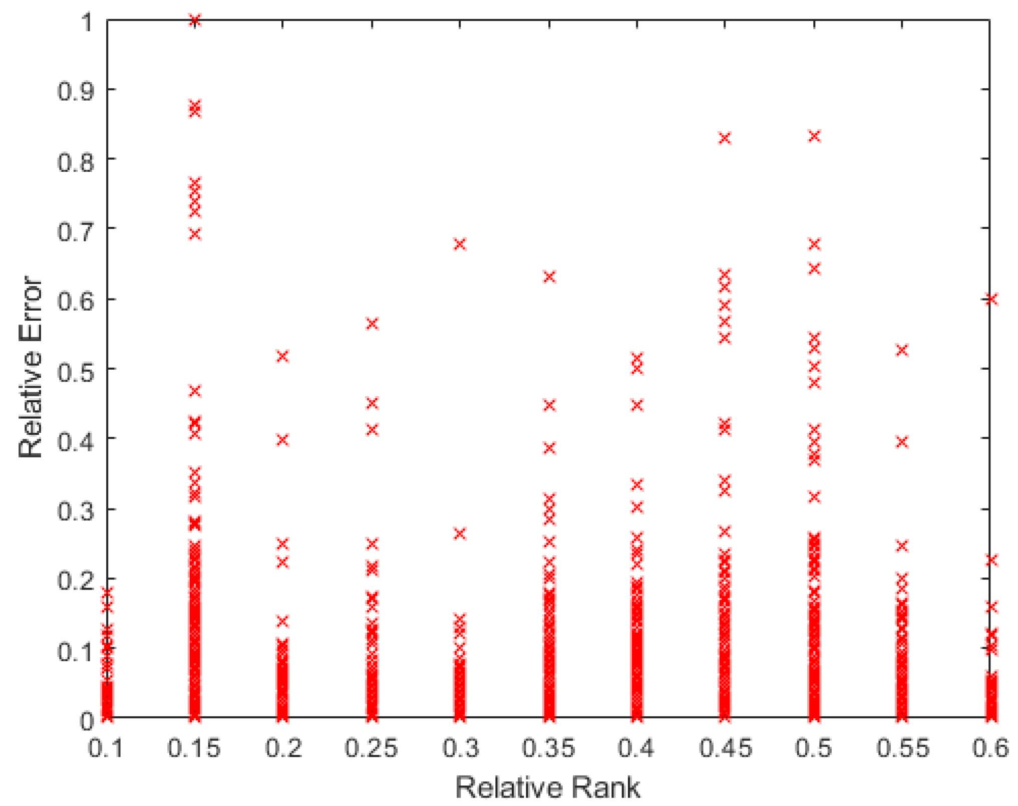
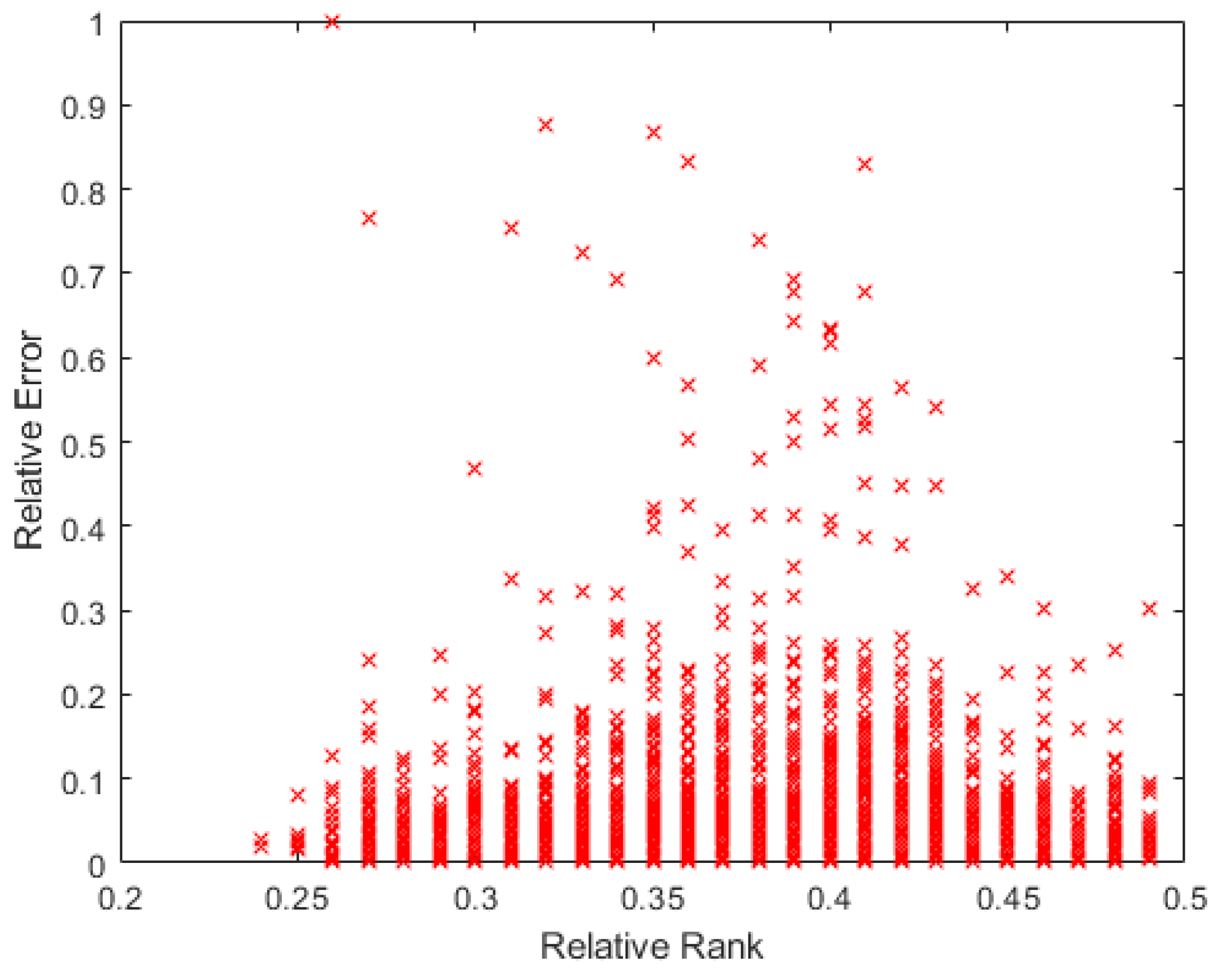
On the contrary, the ReLU layers show different ranks for different patterns. On Figure 14, it can be seen that the maximum reached relative rank of the layer with this batch of patterns is 0.6; being a 20 × 20 matrix of weights, its rank will be 12. There is no particular distribution of the error according to the rank.

In Figure 15, the same distribution as before is shown, but for the X₄ layer. In this case, the maximum relative rank does not reach 0.5, being a 100 × 100 matrix, so the maximum rank is then less than 50. As in the previous case, this distribution offers no particular tendency of the error to concentrate on the lower ranks.

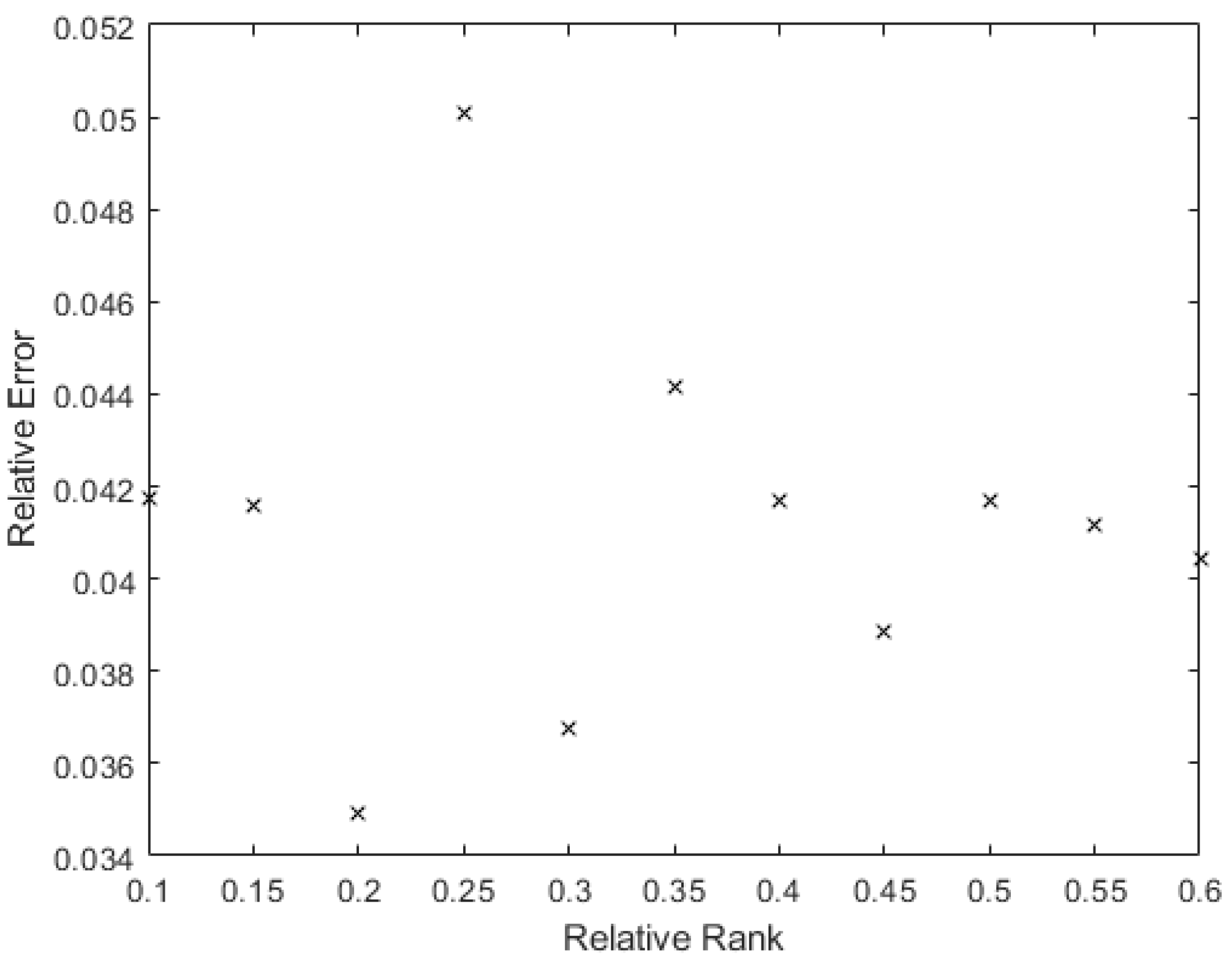
Additionally, just to ensure that there is no relationship between the error and the rank of the ReLU, the average value of the error for each value of the rank was taken. Figure 16 shows this for the X₂ layer.

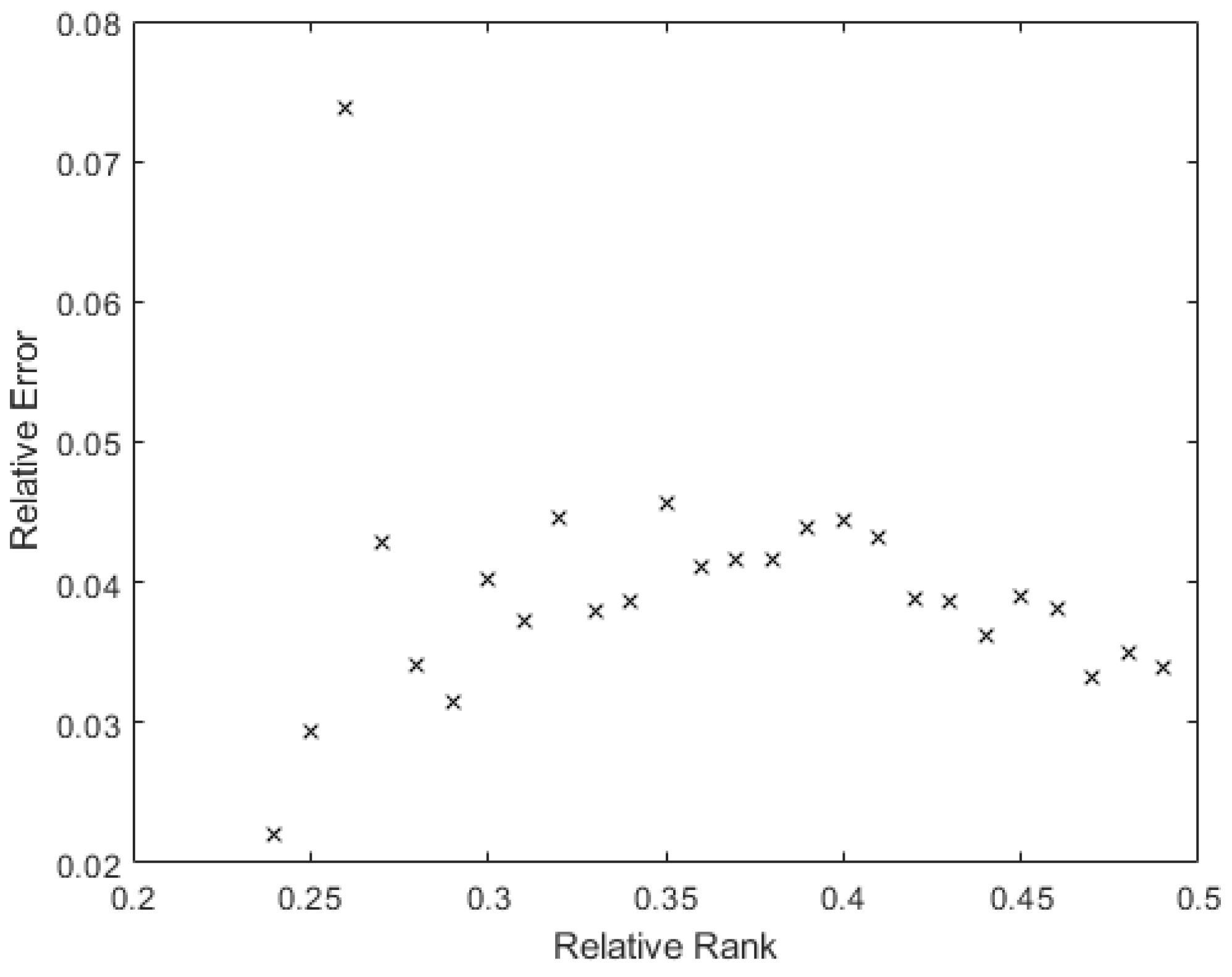
In Figure 17, the average error for X₂ is shown. There is no clear dominance of the higher error in the lower rank; the smallest rank has the smallest average associated error, but there is a trend to reduce the average error in the higher ranks.

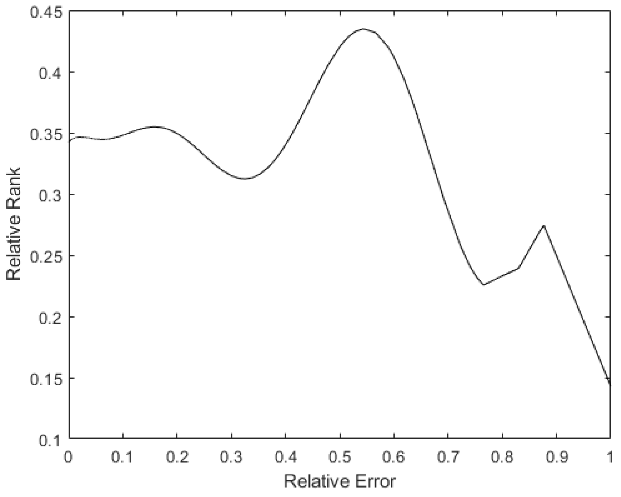
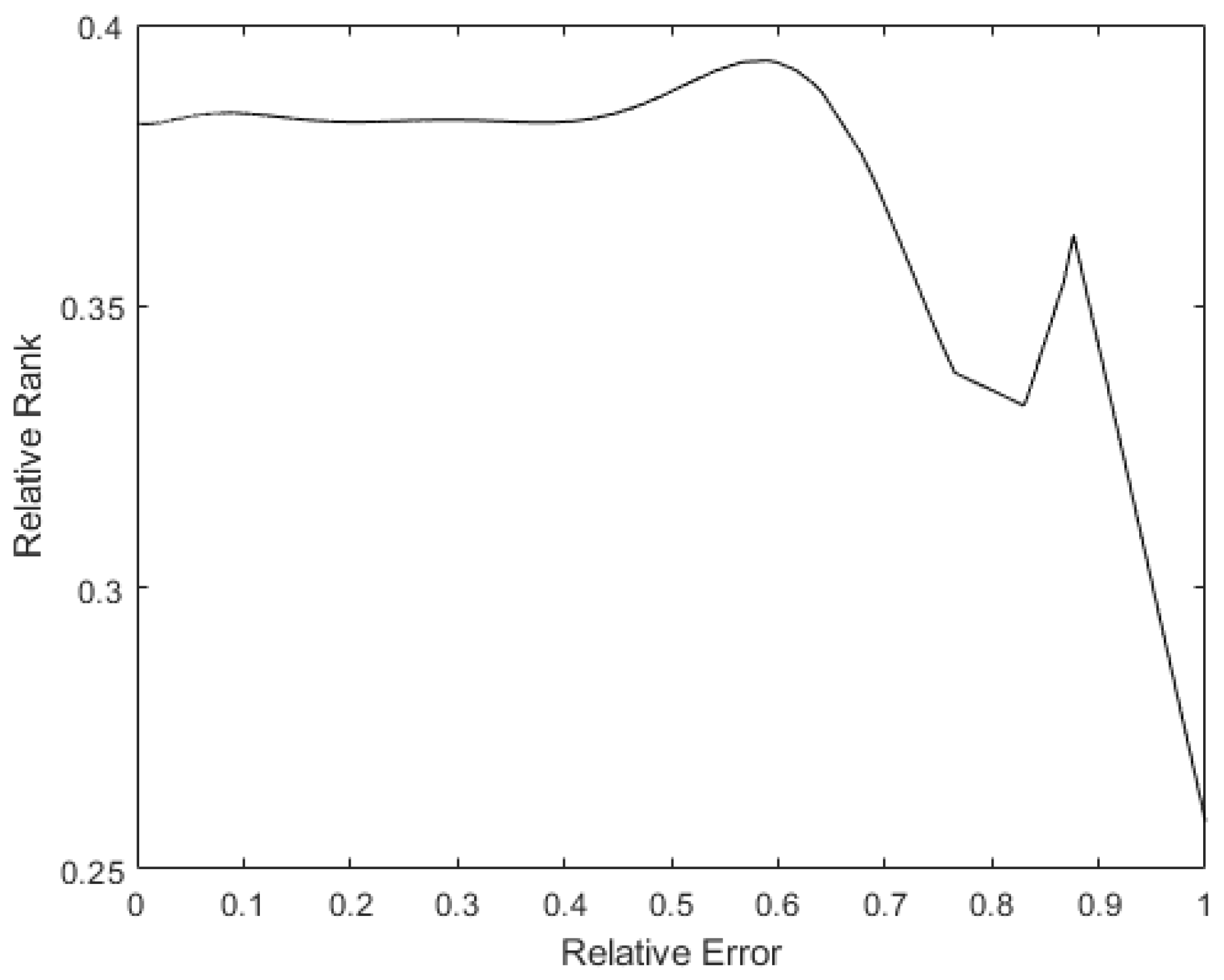
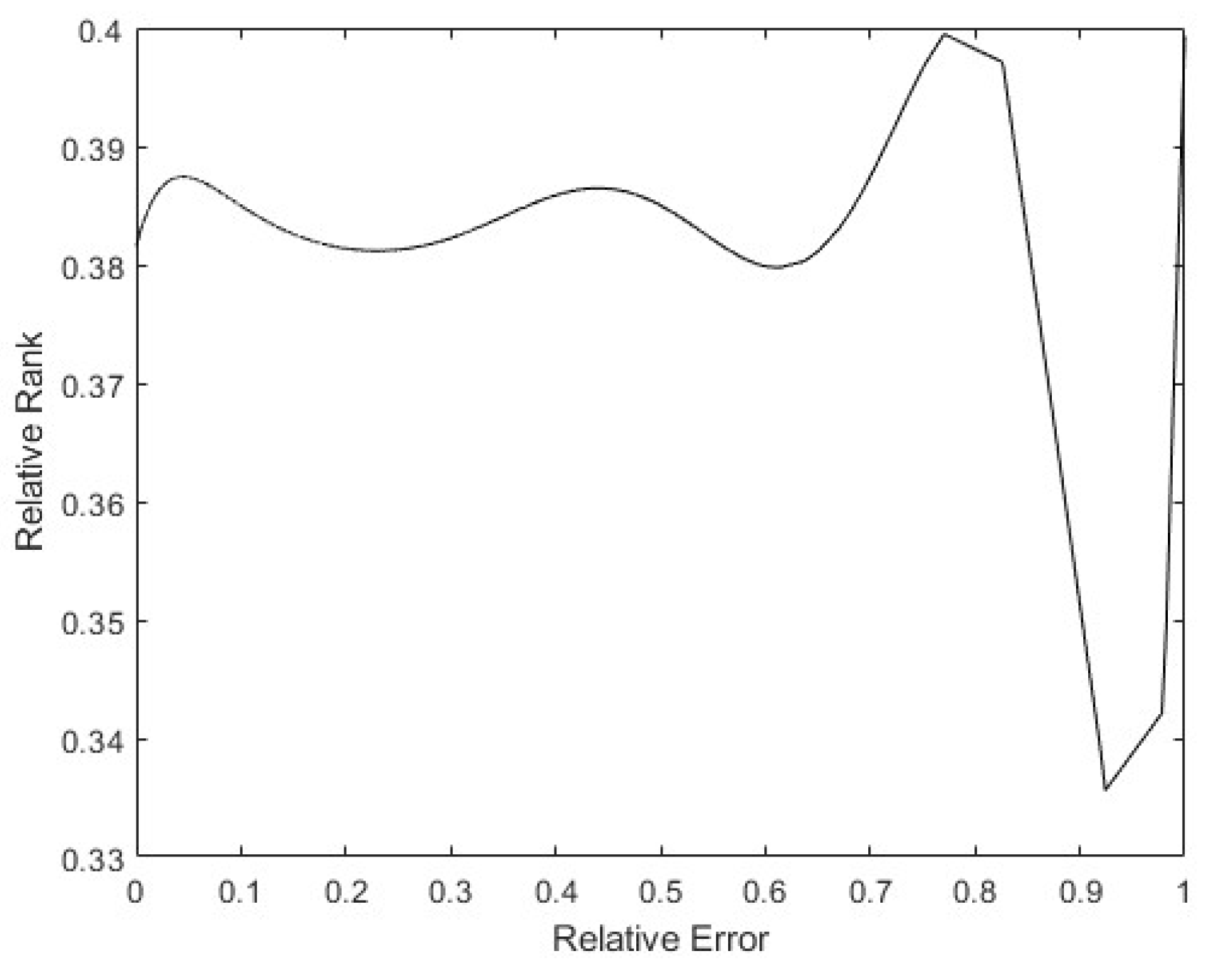
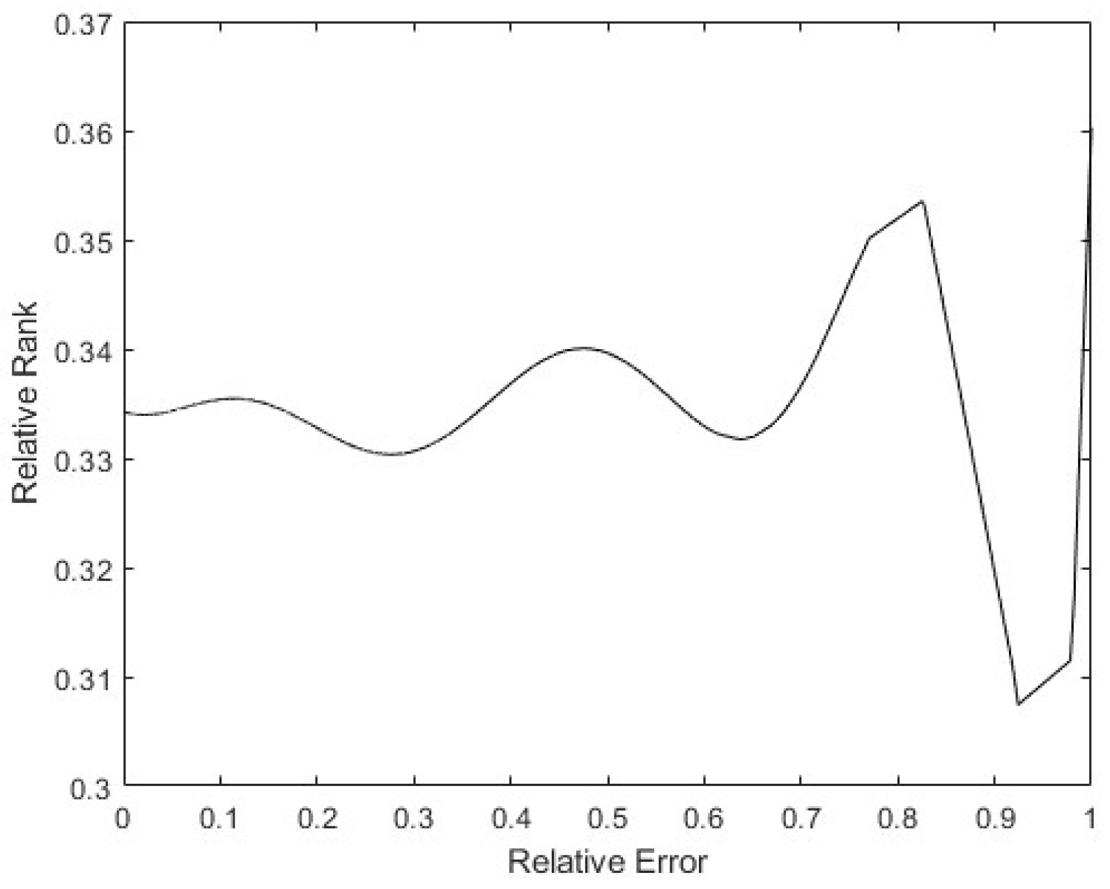
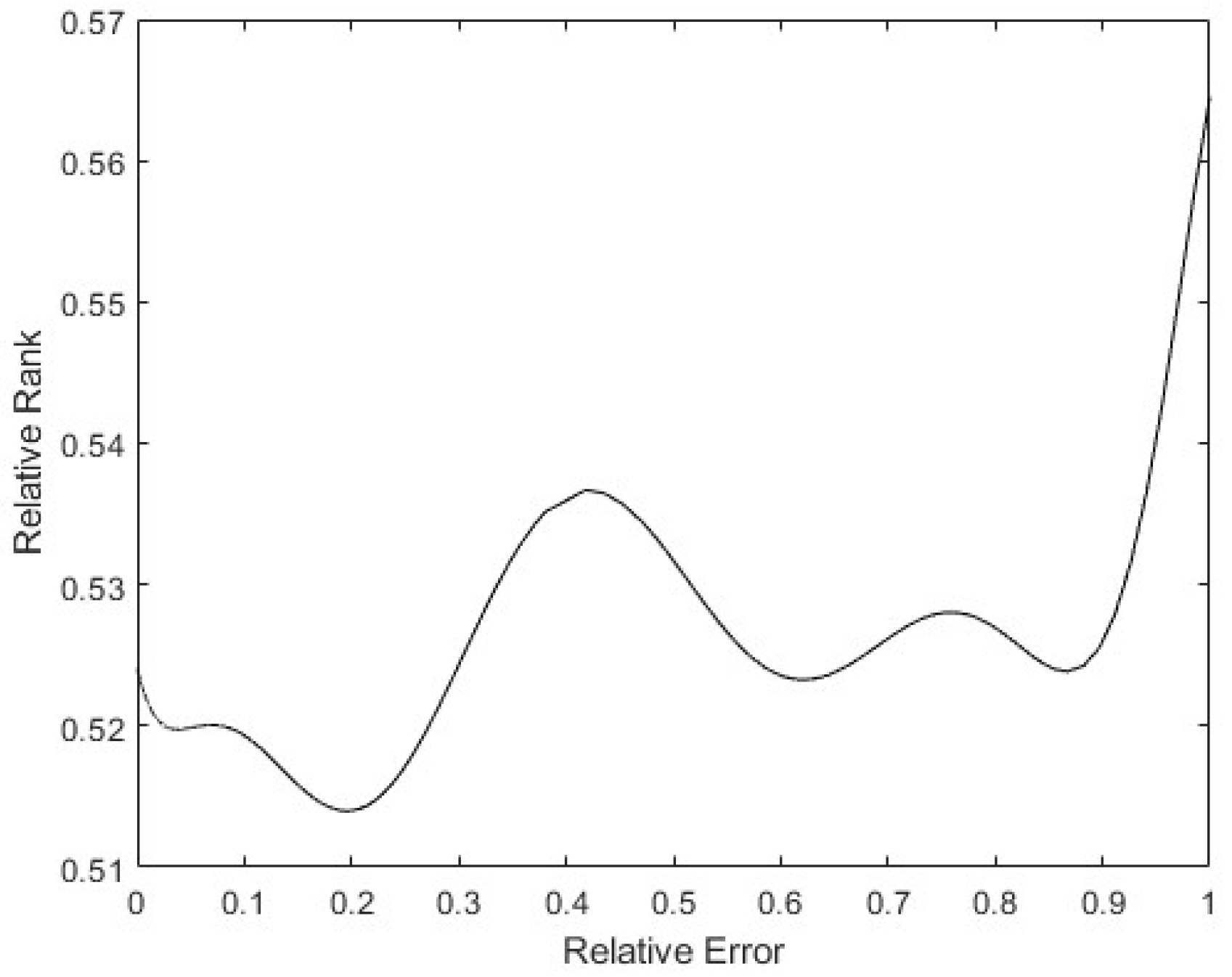
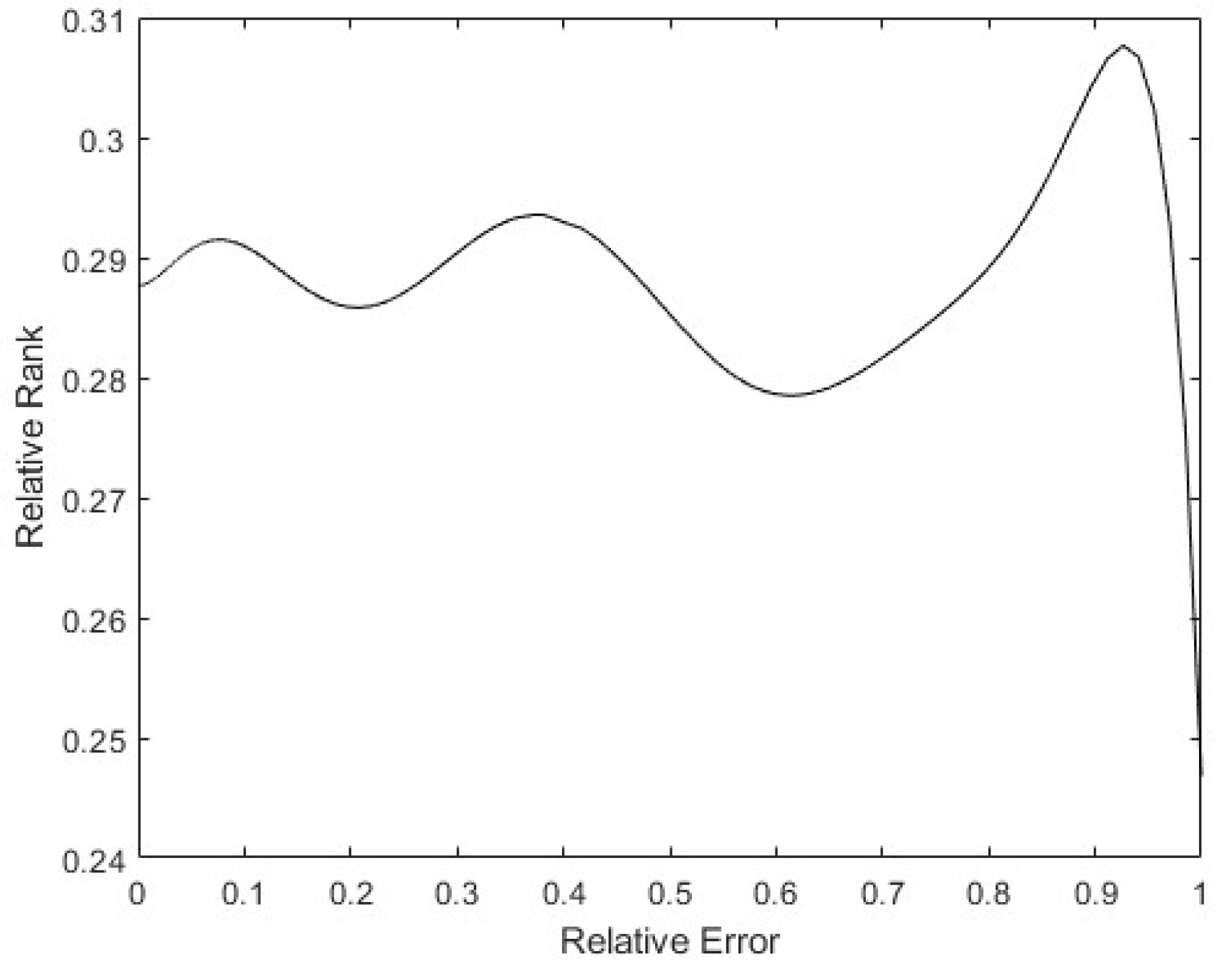
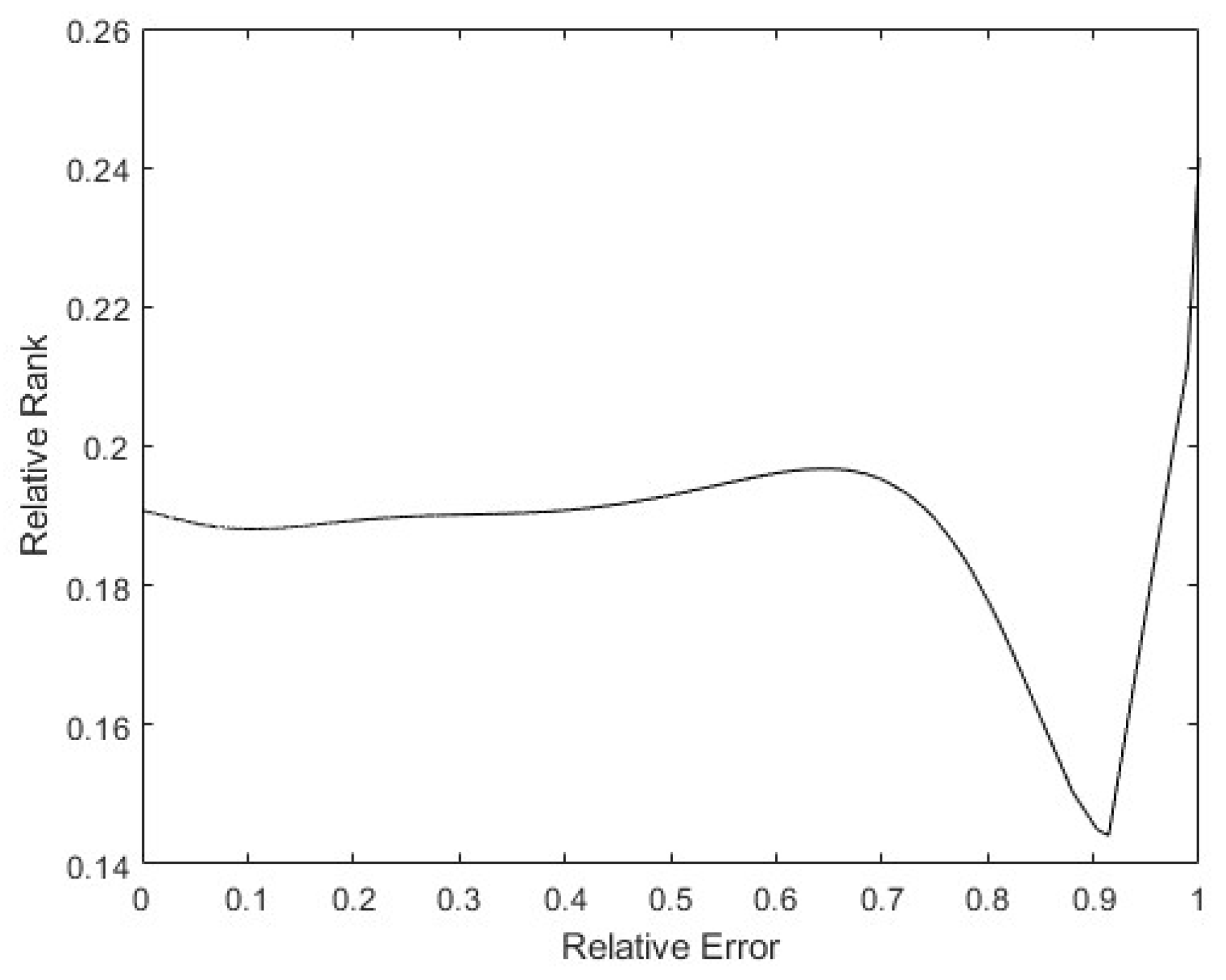
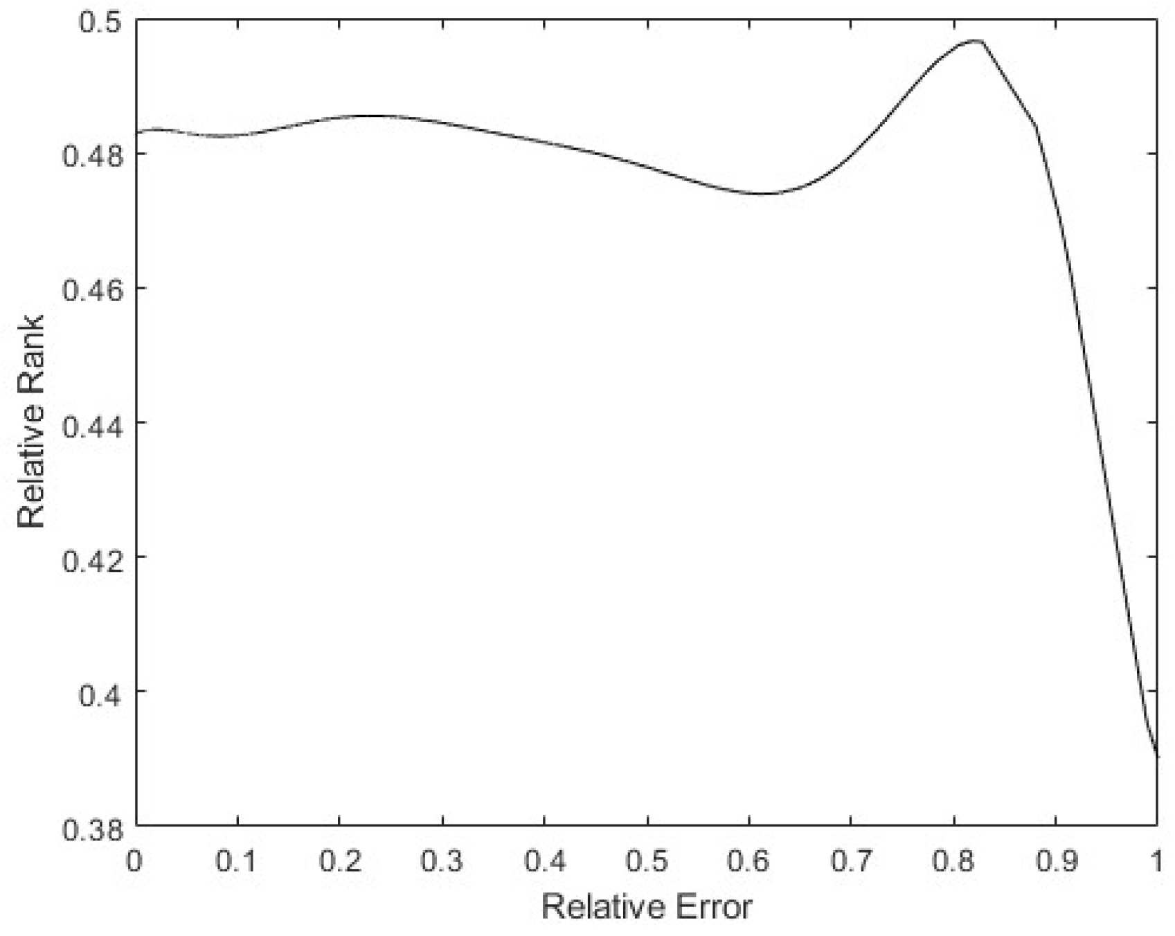
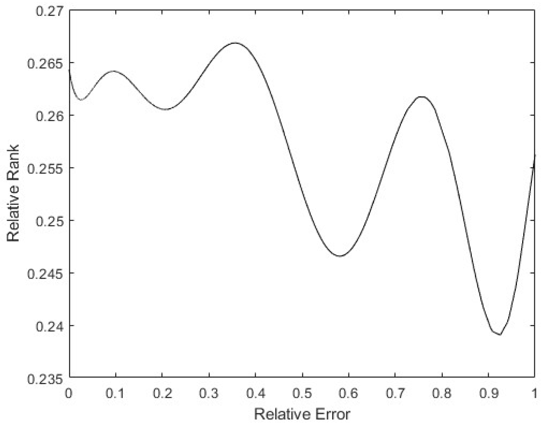
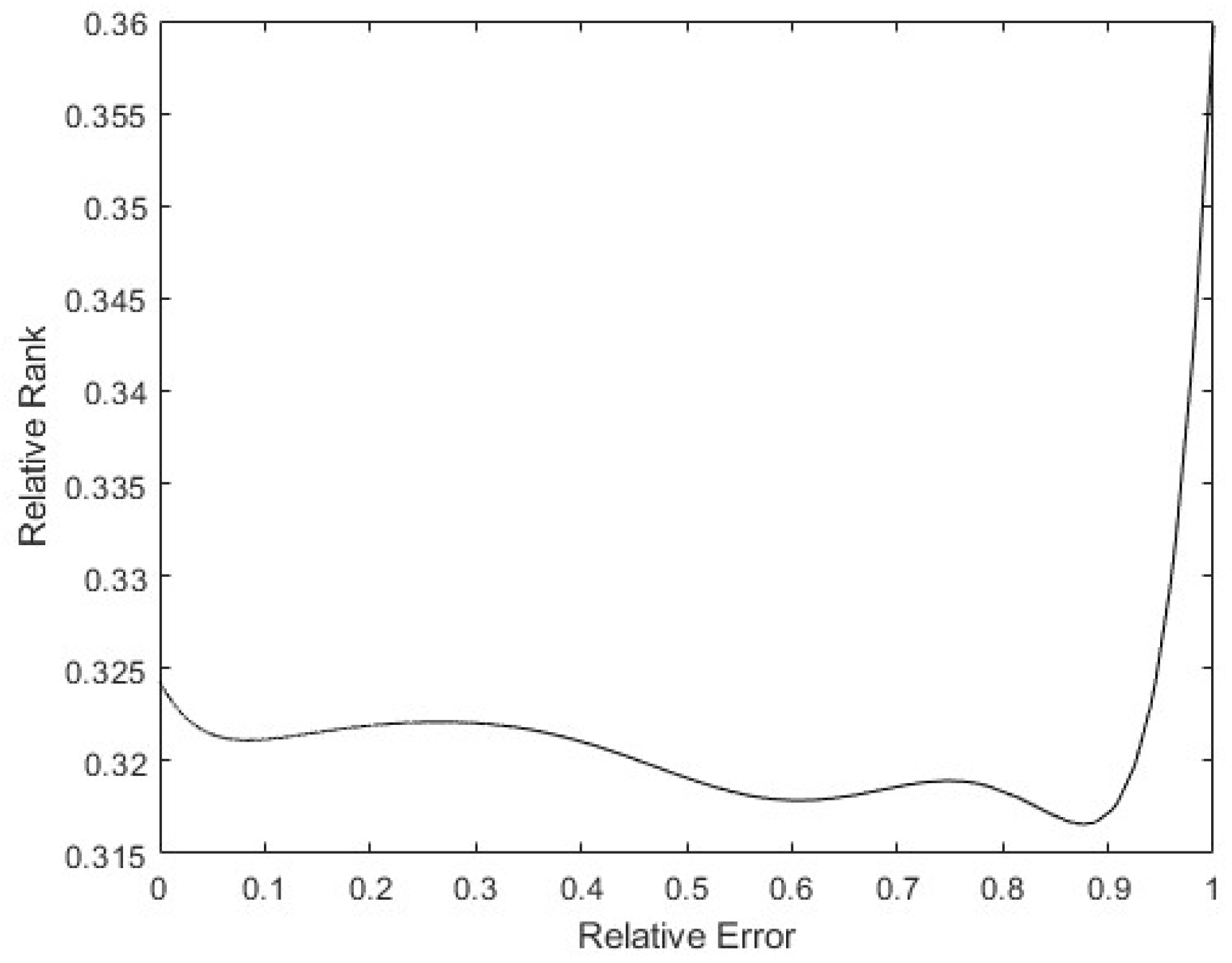
Finally, to see whether the rank of the layer was a function of the relative error of the patterns, a 9th degree polynomial regression was performed with all the data obtained. In Figure 18, it can be seen that the tendency of the rank is to be lower the higher the pattern errors are, with the rank’s minimum on the maximum error. Additionally, there is a maximum in the middle error zone, probably caused by patterns that show the opposite direction gradient, as explained before. These have more information, but in the opposite way to the rest of the patterns. The same happens in Figure 19: the bigger the error is, the smaller the rank. The maximum rank is also present in the middle of the error values, appearing to be due to the same causes as mentioned above.

4.1. Results Obtained in Other Benchmark Functions

Some optimisation functions listed in Surjanovic and Bingham’s web page [39] have been used in order to try different target functions with the same network and training batch. This confirms the usability of the proposed method in other circumstances. The DNN used was the same as that used for the previous experiment, starting from the same initial conditions. The training process was also the same as the one explained in the previous experiment.

4.1.1. The Ackley Function

The Ackley function presents local minimum and maximum points and a central absolute minimum located in the [0, 0] position. For use in this case, the resulting target equation is the following:

$$z=-20·e^{\left(-0.2\sqrt{\frac{1}{2}\left(X^2+y^2\right)}\right)}-e^{\left(\frac{1}{2}\left(\cos \left(2\pi x\right)+\cos \left(2\pi y\right)\right)\right)}+20+e ; x,y\in \left[-0.95, 1\right]$$

(12)

where x and y are the inputs of the network and z its output. The following figure, Figure 20, shows the expected output shape of this function for the data range used, as well as the results and error obtained.

After the training process, the worst and best learnt pattern diagrams are shown in Figure 21 and Figure 22. As in the previous case, the relationships of the module in the worst learnt patterns are much bigger than the best learnt ones. The difference with the previous test is that some of the worst learnt patterns show a positive cos(φ), meaning that most of the patterns are aligned with the average learning vector. The most probable case is that training more epochs will result in turning those patterns into negative ones.

Regarding the relation between the rank and pattern errors of the ReLU layers, the shape is similar to that of the previous experiment. The only particularly different thing is that the rank of the maximum error is higher than the near values. Figure 23 and Figure 24 show these relationships.

4.1.2. Cross-in-Tray Function

This function presents one global maximum in the [0, 0] position and four global minimums located, in this particular case, on the edges of the data rank. The target equation is the following:

$$z=-0.0001{\left(\left|\sin \left(x\right)\ast \sin \left(y\right)\ast e^{\left|100-\frac{\sqrt{x^2+y^2}}{\pi }\right|}\right|+1\right)}^{0.1} ; x,y\in \left[-0.95, 1\right],$$

(13)

where x and y are the inputs of the network and z its output. The expected output of the training, the obtained results and the error are shown in Figure 25.

In this case, all the best and worst learnt patterns have an expected behaviour as far as their module and angle aspect are concerned. All the worst learnt patterns had a negative low cos(φ) and a big module relationship with the average value, while the best learnt are mostly aligned and the relationship of their modules to the average is much smaller than the worst learnt ones. Figure 26 and Figure 27 show the results obtained in this matter.

Considering the error/rank relationship, X₄ has a completely predictable behaviour; X₂ tends to have a higher rank while the error increases. This means that the gradient of the Loss function for this pattern has a misalignment with respect to the average gradient of all the patterns in that layer. These ranks are displayed in Figure 28 and Figure 29.

4.1.3. The De Jong Function Number 5

This function, for the range of inputs used, offers a flat minimum surface and rises at the edges. The target equation is the following:

$$\begin{gathered} z=\left(0.002+{\displaystyle \sum }_{i=1}^{25}\frac{1}{i+{\left(x-a_{1i}\right)}^6+\left(y-a_{2i}\right)}\right); x,y\in \left[-0.95, 1\right]; \\ a=\left(\begin{array}{ccc}-32& -16& 0\\ -32& -32& -32\end{array}\begin{array}{ccc} 16& 32& -32\\ -32& -32& -16\end{array}\begin{array}{cc}\dots & 0\\ \dots & 32\end{array}\begin{array}{cc} 16& 32\\ 32& 32\end{array}\right), \end{gathered}$$

(14)

where x and y are the inputs of the network and z its output. Figure 30 shows the expected output, the obtained results and the error.

As for the pattern angle and the module relationship, both groups present the expected behaviour. These results are shown in Figure 31 and Figure 32.

In the case of rank/error relationship of the ReLu layers, the situation is similar to the previous example, as the X₂ layer has a positive trend according to the error, revealing once again that there is a pattern with a high error completely misaligned with the average of all the patterns in that layer. In the case of X₄, the behaviour is equivalent to the original example. This can be seen in Figure 33 and Figure 34.

4.1.4. Drop-Wave Function

This function presents several maximum and minimum points, offering many direction changes in the chosen data set. The expected output offers the following equation:

$$z=-\frac{1+cos\left(12\sqrt{x^2+y^2}\right)}{0.5\left(x^2+y^2\right)+2}; x,y\in \left[-0.95, 1\right],$$

(15)

where x and y are the inputs of the network and z its output. In this case, the DNN used is clearly insufficient for the target function in the data range exhibited; it is not able to learn correctly most of the target data. Figure 35 shows this issue.

As can be seen, the resulting shape can barely be distinguished from the results after the training has been performed. As for the behaviour of the patterns, however, the module relationship and the angle both have the expected behaviours. The results are shown in Figure 36 and Figure 37.

As for the rank/error relationship, in Figure 38 and Figure 39, it is once again clear from the X₄ layer that there is a totally misaligned pattern that makes the rank rise when there is a higher error.

5. Future Work

There are different possibilities to move forwards from here:

• To improve the SGD algorithm. One possible option is to normalise the gradient from one layer to the next, thus allowing the error information to be distributed at the same rhythm over the entire the network.
• To analyse when to use the SWARM intelligence as algorithms; using for example shallow networks.
• To use pruning algorithms as a basis in order to identify the weakest parts of the network and then reinforce them.

6. Conclusions

Several processes have been identified where the SGD-based algorithm can show problems in different learning patterns. The first is related to the relative rank of the Jacobian matrix that has to be calculated in learning algorithm steps. The second process is related to the misalignment of the gradient of a certain pattern compared to the average gradient of the whole learning batch of patterns. Some techniques have been identified to detect these processes, proposing different alternatives to avoid their influence on the network. If these problems cannot be solved by regularisation techniques such as dropout, neural network architecture changes are proposed, such as residual branches on the network. These branches would increase the relative rank of the Jacobian matrices. Another possible solution could be to add more complexity to the FC layers of the network, so more accurate data could be stored on them; this would enable learning of other details of the patterns that are dismissed, while also learning in a smaller network. Thus, the patterns that require other patterns to be forgotten are less likely to appear. It is not always easy to determine the cause of the incorrect learning of a DNN as there can be more than one reason for it. Changing the architecture or the training algorithm, obtaining more data, or using data-augmentation techniques can provide possible solutions for other issues that might appear.

References

- Shi, S.; Wang, Q.; Zhao, K.; Tang, Z.; Wang, Y.; Huang, X.; Chu, X. A Distributed Synchronous SGD Algorithm with Global Top-k Sparsification for Low Bandwidth Networks. In Proceedings of the 2019 IEEE 39th International Conference on Distributed Computing Systems (ICDCS), Dallas, TX, USA, 7–10 July 2019; pp. 2238–2247. [Google Scholar]
- Lai, G.; Li, F.; Feng, J.; Cheng, S.; Cheng, J. A LPSO-SGD Algorithm for the Optimization of Convolutional Neural Network. In Proceedings of the 2019 IEEE Congress on Evolutionary Computation (CEC), Wellington, New Zealand, 10–13 June 2019; pp. 1038–1043. [Google Scholar]
- Meng, Q.; Chen, W.; Wang, Y.; Ma, Z.-M.; Liu, T.-Y. Convergence Analysis of Distributed Stochastic Gradient Descent with Shuffling. Neurocomputing 2019, 337, 46–57. [Google Scholar] [CrossRef]
- Ming, Y.; Zhao, Y.; Wu, C.; Li, K.; Yin, J. Distributed and Asynchronous Stochastic Gradient Descent with Variance Reduction. Neurocomputing 2018, 281, 27–36. [Google Scholar] [CrossRef]
- Sharma, A. Guided Parallelized Stochastic Gradient Descent for Delay Compensation. Appl. Soft Comput. 2021, 102, 107084. [Google Scholar] [CrossRef]
- Wang, J.; Liang, H.; Joshi, G. Overlap Local-SGD: An Algorithmic Approach to Hide Communication Delays in Distributed SGD. In Proceedings of the ICASSP 2020 IEEE International Conference on Acoustics, Speech and Signal Processing (ICASSP), Barcelona, Spain, 4–8 May 2020; pp. 8871–8875. [Google Scholar]
- Kobayashi, T. SCW-SGD: Stochastically Confidence-Weighted SGD. In Proceedings of the 2020 IEEE International Conference on Image Processing (ICIP), Abu Dhabi, United Arab Emirates, 25–28 October 2020; pp. 1746–1750. [Google Scholar]
- Yang, X.; Zheng, X.; Gao, H. SGD-Based Adaptive NN Control Design for Uncertain Nonlinear Systems. IEEE Trans. Neural Netw. Learn. Syst. 2018, 29, 5071–5083. [Google Scholar] [CrossRef]
- Zhang, N.; Wu, W.; Zheng, G. Convergence of Gradient Method with Momentum for Two-Layer Feedforward Neural Networks. IEEE Trans. Neural Netw. 2006, 17, 522–525. [Google Scholar] [CrossRef]
- Lenka, S.K.; Mohapatra, A.G. Gradient Descent with Momentum Based Neural Network Pattern Classification for the Prediction of Soil Moisture Content in Precision Agriculture. In Proceedings of the 2015 IEEE International Symposium on Nanoelectronic and Information Systems, Indore, India, 21–23 December 2015; pp. 63–66. [Google Scholar]
- Zhang, N. Momentum Algorithms in Neural Networks and the Applications in Numerical Algebra. In Proceedings of the 2011 2nd International Conference on Artificial Intelligence, Management Science and Electronic Commerce (AIMSEC), Deng Feng, China, 8–10 August 2011; pp. 2192–2195. [Google Scholar]
- Kim, P. MATLAB Deep Learning; Apress: Berkeley, CA, USA, 2017; ISBN 978-1-4842-2844-9. [Google Scholar]
- Torres, J. Python Deep Learning; 1.0.; Marcombo: Barcelona, Spain, 2020; ISBN 978-84-267-2828-9. [Google Scholar]
- Wani, M.A.; Afzal, S. A New Framework for Fine Tuning of Deep Networks. In Proceedings of the 2017 16th IEEE International Conference on Machine Learning and Applications (ICMLA), Cancun, Mexico, 18–21 December 2017; pp. 359–363. [Google Scholar]
- He, C.; Ma, M.; Wang, P. Extract Interpretability-Accuracy Balanced Rules from Artificial Neural Networks: A Review. Neurocomputing 2020, 387, 346–358. [Google Scholar] [CrossRef]
- Gudise, V.G.; Venayagamoorthy, G.K. Comparison of Particle Swarm Optimization and Backpropagation as Training Algorithms for Neural Networks. In Proceedings of the 2003 IEEE Swarm Intelligence Symposium, Indianapolis, IN, USA, 26 April 2003; pp. 110–117. [Google Scholar] [CrossRef]
- Sari, Y. Performance Evaluation of the Various Training Algorithms and Network Topologies in a Neural-Network-Based Inverse Kinematics Solution for Robots. Int. J. Adv. Robot. Syst. 2014, 11, 64. [Google Scholar] [CrossRef]
- Chen, J.-F.; Do, Q.H.; Hsieh, H.-N. Training Artificial Neural Networks by a Hybrid PSO-CS Algorithm. Algorithms 2015, 8, 292–308. [Google Scholar] [CrossRef]
- Devi, R.M.; Kuppuswami, S.; Suganthe, R.C. Fast Linear Adaptive Skipping Training Algorithm for Training Artificial Neural Network. Math. Probl. Eng. 2013, 2013, 346949. [Google Scholar] [CrossRef]
- Shallue, C.J.; Lee, J.; Antognini, J.; Sohl-Dickstein, J.; Frostig, R.; Dahl, G.E. Measuring the Effects of Data Parallelism on Neural Network Training. J. Mach. Learn. Res. 2019, 20, 1–49. [Google Scholar]
- Cheng, X.; Feng, Z.-K.; Niu, W.-J. Forecasting Monthly Runoff Time Series by Single-Layer Feedforward Artificial Neural Network and Grey Wolf Optimizer. IEEE Access 2020, 8, 157346–157355. [Google Scholar] [CrossRef]
- Ho, L.V.; Nguyen, D.H.; Mousavi, M.; De Roeck, G.; Bui-Tien, T.; Gandomi, A.H.; Wahab, M.A. A Hybrid Computational Intelligence Approach for Structural Damage Detection Using Marine Predator Algorithm and Feedforward Neural Networks. Comput. Struct. 2021, 252, 106568. [Google Scholar] [CrossRef]
- Bairathi, D.; Gopalani, D. Salp Swarm Algorithm (SSA) for Training Feed-Forward Neural Networks. In Soft Computing for Problem Solving; Bansal, J.C., Das, K.N., Nagar, A., Deep, K., Ojha, A.K., Eds.; Springer: Singapore, 2019; pp. 521–534. [Google Scholar]
- Milosevic, S.; Bezdan, T.; Zivkovic, M.; Bacanin, N.; Strumberger, I.; Tuba, M. Feed-Forward Neural Network Training by Hybrid Bat Algorithm. In Modelling and Development of Intelligent Systems; Simian, D., Stoica, L.F., Eds.; Springer International Publishing: Cham, Switzerland, 2021; pp. 52–66. [Google Scholar]
- Erkaymaz, O. Resilient Back-Propagation Approach in Small-World Feed-Forward Neural Network Topology Based on Newman–Watts Algorithm. Neural Comput. Appl. 2020, 32, 16279–16289. [Google Scholar] [CrossRef]
- Najafi, A.; Maeda, S.I.; Koyama, M.; Miyato, T. Robustness to Adversarial Perturbations in Learning from Incomplete Data. In Advances in Neural Information Processing Systems; MIT Press: Cambridge, MA, USA, 2019; Volume 32. [Google Scholar]
- Choudhury, S.J.; Pal, N.R. Imputation of Missing Data with Neural Networks for Classification. Knowl. Based Syst. 2019, 182, 104838. [Google Scholar] [CrossRef]
- Zhang, Z.; Yang, P.; Ren, X.; Su, Q.; Sun, X. Memorized Sparse Backpropagation. Neurocomputing 2020, 415, 397–407. [Google Scholar] [CrossRef]
- Blanco, A.; Delgado, M.; Pegalajar, M.C. A Real-Coded Genetic Algorithm for Training Recurrent Neural Networks. Neural Netw. 2001, 14, 93–105. [Google Scholar] [CrossRef]
- Doshi, D.; He, T.; Gromov, A. Critical Initialization of Wide and Deep Neural Networks through Partial Jacobians: General Theory and Applications to LayerNorm. arXiv 2021. [Google Scholar] [CrossRef]
- Wilamowski, B.M.; Cotton, N.J.; Kaynak, O.; Dündar, G. Computing Gradient Vector and Jacobian Matrix in Arbitrarily Connected Neural Networks. IEEE Trans. Ind. Electron. 2008, 55, 3784–3790. [Google Scholar] [CrossRef]
- Jean, S.; Cho, K.; Memisevic, R.; Bengio, Y. On Using Very Large Target Vocabulary for Neural Machine Translation. arXiv 2015. [Google Scholar] [CrossRef]
- Tanaka, H.; Kunin, D.; Yamins, D.L.K.; Ganguli, S. Pruning Neural Networks without Any Data by Iteratively Conserving Synaptic Flow. arXiv 2020. [Google Scholar] [CrossRef]
- Ioffe, S.; Szegedy, C. Batch Normalization: Accelerating Deep Network Training by Reducing Internal Covariate Shift. In Proceedings of the 32nd International Conference on Machine Learning; Bach, F., Blei, D., Eds.; PMLR: Lille, France, 2015; Volume 37, pp. 448–456. [Google Scholar]
- Taheri, S.; Toygar, Ö. On the Use of DAG-CNN Architecture for Age Estimation with Multi-Stage Features Fusion. Neurocomputing 2019, 329, 300–310. [Google Scholar] [CrossRef]
- Cheng, F.; Zhang, H.; Yuan, D.; Sun, M. Leveraging Semantic Segmentation with Learning-Based Confidence Measure. Neurocomputing 2019, 329, 21–31. [Google Scholar] [CrossRef]
- Macêdo, D.; Zanchettin, C.; Oliveira, A.L.I.; Ludermir, T. Enhancing Batch Normalized Convolutional Networks Using Displaced Rectifier Linear Units: A Systematic Comparative Study. Expert Syst. Appl. 2019, 124, 271–281. [Google Scholar] [CrossRef]
- Wang, J.; Li, S.; An, Z.; Jiang, X.; Qian, W.; Ji, S. Batch-Normalized Deep Neural Networks for Achieving Fast Intelligent Fault Diagnosis of Machines. Neurocomputing 2019, 329, 53–65. [Google Scholar] [CrossRef]
- Surjanovic, S.; Bingham, D. Virtual Library of Simulation Experiments: Test Functions and Datasets. Available online: https://www.sfu.ca/~ssurjano/index.html (accessed on 6 August 2022).
Figure 1.
General representation of neural network layers.
Figure 2.
General representation of the size of the components of the equation.
Figure 3.
Representation of the network under study.
Figure 4.
Jacobians and their sizes, taking the network from the input layer.
Figure 5.
Jacobians and their sizes, taking the network from the third layer.
Figure 6.
Component sizes, taking the lattice from the output layer.
Figure 7.
A simple representation of the created feedforward neural network.
Figure 8.
Results of the training.
Figure 9.
20 worst learnt patterns cos(φ) in the first column and relationship to the average on the second. The output layer is represented in the first row, the intermediate layer in the second and the input layer in the third.
Figure 10.
20 best learnt patterns cos(φ) in the first column and the relationship to the average in the second. The output layer is represented in the first row, the intermediate layer in the second and the input layer in the third.
Figure 11.
Unified worst learnt patterns cos(φ) on the left and the relationship to the average on the right.
Figure 12.
Unified best learnt patterns cos(φ) on the left and the relationship to the average on the right.
Figure 13.
FC layers’ patterns distribution according the Relative Rank and Relative Error.
Figure 14.
Pattern distribution according to their Relative Error and Relative Rank in X2.
Figure 15.
Pattern distribution according to their Relative Error and Relative Rank in X4.
Figure 16.
Average value of the relative error according to the relative rank in X2.
Figure 17.
Average value of the relative error according to the relative rank in X4.
Figure 18.
Polynomial regression of relative rank to relative error on X2.
Figure 19.
Polynomial regression of relative rank to relative error on X4.
Figure 20.
Expected output of the DNN for the Ackley function on the left, the obtained results in the middle and the error on the right.
Figure 21.
20 worst learnt unified patterns cos(φ) on the left and the relationship to the average on the right.
Figure 22.
20 best learnt unified patterns cos(φ) on the left and the relationship to the average on the right.
Figure 23.
Figure 24.
Figure 25.
Expected output of the DNN for the Cross-in-Tray function on the left, the obtained results in the middle and the error on the right.
Figure 26.
Figure 27.
Figure 28.
Figure 29.
Figure 30.
Expected output of the DNN for the De Jong function on the left, the obtained results in the middle and the error on the right.
Figure 31.
Figure 32.
Figure 33.
Figure 34.
Figure 35.
Expected output of the DNN for the Drop-Wave function on the left, the obtained results in the middle and the error on the right.
Figure 36.
Figure 37.
Figure 38.
Figure 39.