Analytical Investigations into Anomalous Diffusion Driven by Stress Redistribution Events: Consequences of Lévy Flights

Abstract

This research is concerned with developing a generalised diffusion equation capable of describing diffusion processes driven by underlying stress-redistributing type events. The work utilises the development of an appropriate continuous time random walk framework as a foundation to consider a new generalised diffusion equation. While previous work has explored the resulting generalised diffusion equation for jump-timings motivated by stick-slip physics, here non-Gaussian probability distributions of the jump displacements are also considered, specifically Lévy flights. This work illuminates several features of the analytic solution to such a generalised diffusion equation using several known properties of the Fox H function. Specifically demonstrated are the temporal behaviour of the resulting position probability density function, and its normalisation. The reduction of the proposed form to expected known solutions upon the insertion of simplifying parameter values, as well as a demonstration of asymptotic behaviours, is undertaken to add confidence to the validity of this equation. This work describes the analytical solution of such a generalised diffusion equation for the first time, and additionally demonstrates the capacity of the Fox H function and its properties in solving and studying generalised Fokker–Planck equations.

1. Introduction

Diffusion is a widespread phenomena, occurring across a vast array of physical systems. The study of diffusive systems in a physical and mathematical sense may be divided into those exhibiting Gaussian or non-Gaussian behaviours. These two classes of diffusive process are also often referred to as normal (Gaussian) and anomalous (non-Gaussian) diffusion, although there have been more recent works to suggest some overlap between these classes [1,2]. Classification of a process into one of the two categories is based on the value of the characteristic exponent of the time dependence of the second moment of the probability density function (PDF). In the instance where the process occurs in a spatially symmetric manner, the second moment and mean squared displacement are equivalent and thus,

$${\mu }_2\left(t\right)=\langle x^2\rangle \left(t\right)=t^{\gamma }.$$

(1)

In Equation (1), $\gamma$ plays the role of the characteristic exponent. Normal diffusion is said to occur for $\gamma =1$ and when $\gamma \ne 1$ the process is described as anomalous. Anomalous diffusion is abundant amongst the natural world, and as a consequence of this prevalence it has been the subject of widespread study, of which there is a rich history. As specific examples, it has been observed in charge carrier transport in amorphous semiconductors [3,4], in flow in porous systems [5], in quantum optics [6,7], as well as many other systems [8,9]. In a mathematical context, two predominant branches of study exist, one extends from the works of Langevin, aiming to produce a stochastic description of a single trajectory. The second branch is concerned with the time evolution of the entire ensemble of a process, with early works in this vain formulated by the likes of Fokker, Planck, and Smoluchowski [10].

In prior work by the authors, a generalized diffusion equation was derived from an underlying continuous time random walk (CTRW) [11] that possessed a timing distribution associated with stress redistributing systems. The intention of that work was to explore the ability of fractional or non-Markovian models to describe dynamics within physical systems with stress redistributing features (such as those found in earthquake dynamics, physical gels, and many stick-slip models). It could be said that the mentioned work focused on the temporal implications of stress redistribution for resulting diffusive processes. The present research explores the spatial implications which follow from stress re-distributing processes driving anomalous diffusion. In order to capture these spatial features, we employ non-Gaussian distributions of the displacements in the underlying CTRW framework. Specifically the class of probability density functions known as stable Lévy distributions are inserted for the displacement probability densities in the underlying CTRW.

This article will be structured as follows, Section 2 will give a brief overview of the underlying CTRW framework, Section 3 outlines the consequences of incorporating Lévy stable probability densities in the CTRW in terms of the resulting generalised diffusion equation, the probability density current, and the displacement PDF. Section 3 finishes with the demonstration of the normalisation and reduction properties of the obtained solution to the generalised diffusion equation. Finally, Section 4 covers the key findings and provides some concluding remarks.

2. CTRW

The CTRW framework was first described by Weiss and Montroll, and has been employed in the studies of a number of stochastic processes [12]. The CTRW is built up from the stochastic exploration of a walker through space, where the displacements x are interrupted by waiting times t. These variables are drawn from a continuous probability density function (PDF) $\mathsf{\Psi }(x,t)$. In the instance that there exists no correlations between the size of the displacement and the waiting time (decoupled CTRW), the following expressions hold

$$\lambda \left(x\right)={\int }_0^{\infty }\mathsf{\Psi }(x,t)dt$$

(2)

$$\omega \left(t\right)={\int }_{-\infty }^{\infty }\mathsf{\Psi }(x,t)dx,$$

(3)

where $\lambda \left(x\right)$ and $\omega \left(t\right)$ are the step-length and waiting time PDFs, respectively. The decoupled framework allows $\mathsf{\Psi }(x,t)$ to be factored into the independent distributions $\lambda \left(x\right)$ and $\omega \left(t\right)$. From these distributions, an arrival PDF, $\eta (x,t)$ describing the probability density of a walker arriving at various positions x in time t, may be constructed. The PDF $\eta (x,t)$ is defined as,

$$\eta (x,t)={\int }_{-\infty }^{\infty }{\int }_0^t\eta (x^{\prime },t^{\prime })\lambda (x-x^{\prime })\omega (t-t^{\prime })d{t}^{\prime }d{x}^{\prime }+\delta \left(x\right)\delta \left(t\right).$$

(4)

The first term of Equation (4) describes the probability associated with a walker at $x^{\prime }$ at time, $t^{\prime }$ having made a jump of length $x-x^{\prime }$ in the remaining time $t-t^{\prime }$, summed over all x and all causally relevant t. Whilst the second term represents the initial conditions, here at time $t=0$ the walker is localized at a position defined by $\delta \left(x\right)$. The position PDF, $P(x,t)$ is then defined as the probability density of arriving and remaining at a position x at time t, defined as

$$P(x,t)={\int }_0^t\eta (x,t^{\prime })\mathsf{\Phi }(t-t^{\prime })d{t}^{\prime },$$

(5)

where $\mathsf{\Phi }\left(t\right)$ is referred to as the survival PDF which provides the probability density for a waiting time longer than t, defined as

$$\mathsf{\Phi }\left(t\right)=1-{\int }_0^t\omega \left(t^{\prime }\right)d{t}^{\prime }.$$

(6)

The typical progress from this point is to pass into the Fourier–Laplace space. This simplifies the expressions through the known transform properties of convolutions [13]. Transforming Equations (4) and (6), then substituting them into the Fourier–Laplace equivalent of Equation (5), provides the following form for $P(k,u)$ [14],

$$P(k,u)=\frac{1-\widehat{\omega }\left(u\right)}{u}\frac{1}{1-\widehat{\lambda }\left(k\right)\widehat{\omega }\left(u\right)}.$$

(7)

3. Lévy Flight

If the CTRW contains a Lévy stable distribution for the displacements, then such behaviour corresponds to the following Fourier space, small k approximation,

$$\widehat{\lambda }\left(k\right)\sim 1-{\sigma }^{\mu }{\left|k\right|}^{\mu },$$

(8)

with $\mu \in [1,2]$ [15]. The waiting time PDF, $\omega \left(t\right)$ utilised in this work is the gamma distribution, which takes the following functional form,

$$\omega \left(t\right)=\frac{t^{\gamma -1}}{{\tau }^{\gamma }\mathsf{\Gamma }\left(\gamma \right)}exp\left(\frac{-t}{\tau }\right).$$

(9)

Equation (9) has been connected with the timing of stress-redistribution events, motivating its use in the present study [11,16,17]. The PDF $\omega \left(t\right)$ appears in the Laplace space as,

$$\widehat{\omega }\left(u\right)=\frac{1}{{\tau }^{\gamma }{\left(\frac{1}{\tau }+u\right)}^{\gamma }}$$

(10)

Inserting Equations (10) and (8) into Equation (7) yields the following expression for the PDF in the Fourier–Laplace space

$$P(k,u)=\frac{1}{u}·\frac{1}{1+\frac{D_{\gamma ,\mu }{\left|k\right|}^{\mu }}{({(\frac{1}{\tau }+u)}^{\gamma }-\frac{1}{{\tau }^{\gamma }})}},$$

(11)

where $D_{\alpha ,\mu }=\frac{{\sigma }^{\mu }}{{\tau }^{\alpha }}$ is the generalised space-time diffusion coefficient.

3.1. Generalised Diffusion Equation

From Equation (11) we can outline a generalised diffusion equation [18]. The generalised diffusion equation appears as,

$$\frac{\partial }{\partial t}P(x,t)=D_{\alpha ,\mu }\frac{\partial }{\partial t}{\int }_0^{t}exp\left(-\frac{(t-t^{\prime })}{\tau }\right){(t-t^{\prime })}^{\gamma -1}{E}_{\gamma ,\gamma }\left(\frac{{(t-t^{\prime })}^{\gamma }}{{\tau }^{\gamma }}\right)\frac{{\partial }^{\mu }}{{\partial \left|x\right|}^{\mu }}P(x,t^{\prime })d{t}^{\prime },$$

(12)

where, $\frac{{\partial }^{\mu }}{{\partial \left|x\right|}^{\mu }}$ is the Riesz space-fractional derivative [19,20]. The Riesz space-fractional derivative is defined as

$$\frac{{\partial }^{\mu }}{{\partial \left|x\right|}^{\mu }}f\left(x\right)=F^{-1}\left[{\left|k\right|}^{\mu }f\left(k\right)\right]\left(x\right),$$

(13)

which in the x space is (for $1<\mu \le 2$),

$$\frac{{\partial }^{\mu }}{{\partial \left|x\right|}^{\mu }}f\left(x\right)=\frac{-1}{2cos(\pi \mu /2)}\frac{1}{\mathsf{\Gamma }(2-\mu )}\frac{{\partial }^2}{\partial x^2}\left({\int }_{-\infty }^x\frac{f\left(x^{\prime }\right)}{{(x-x^{\prime })}^{\mu -1}}d{x}^{\prime }+{\int }_x^{\infty }\frac{f\left(x^{\prime }\right)}{{(x^{\prime }-x)}^{\mu -1}}d{x}^{\prime }\right).$$

(14)

Equation (12) therefore represents the extension of non-locality to include both temporal and spatial domains.

3.1.1. Probability Density Current

There exists a well known connection between the diffusion equation and the continuity equation. The continuity equation states that the total change in concentration at a particular location (the change in probability density in this case) and the divergence of the concentration current at the same location (probability density current in this case) must be zero, in the instance of a conserved quantity. Another way of expressing this is simply to state that in the instance of a conserved quantity the change in this quantity in a defined region must balance the flow of this quantity into and out of the region, or, more succinctly

$$P_t(x,t)=-\frac{\partial }{\partial x}J(x,t).$$

(15)

where in Equation (15) $J(x,t)$ is the probability density current (PDC). This provides a useful starting point for investigations into how a given generalised diffusion equation varies from the standard or normal case. Writing the PDC in a generalised form consistent with fractional calculus

$$J(x,t)={-}_0{G}_t^{1-\gamma }\frac{{\partial }^{\mu -1}}{{\partial \left|x\right|}^{\mu -1}}P(x,t).$$

(16)

where in Equation (16) the operator ${}_0{G}_t^{1-\gamma }$ is defined as,

$${}_0{G}_t^{1-\gamma }f\left(t\right)=\frac{\partial }{\partial t}{\int }_0^{t}exp\left(-\frac{(t-t^{\prime })}{\tau }\right){(t-t^{\prime })}^{\gamma -1}{E}_{\gamma ,\gamma }\left(\frac{{(t-t^{\prime })}^{\gamma }}{{\tau }^{\gamma }}\right)f\left(t^{\prime }\right)d{t}^{\prime }.$$

(17)

It is no longer accurate to describe the PDC, $J(x,t)$, as moving down the gradient of the PDF. In order to establish precisely to what this generalised PDC is sensitive to, we outline its mathematical relationship connection with the position PDF:

$$J(x,t)={-}_0{G}_t^{1-\gamma }\left[\frac{-1}{cos\left(\frac{\pi \left(\mu -1\right)}{2}\right)}\left({}_{-\infty }{D}_x^{\mu -1}P(x,t)+{}_x{D}_{\infty }^{\mu -1}P(x,t)\right)\right].$$

(18)

where the operators ${}_{-\infty }{D}_x^{\mu -1}$ and ${}_x{D}_{\infty }^{\mu -1}$ in Equation (18) are the left and right Riemann–Liouville fractional derivatives (with $0<\mu -1\le 1$) [21], respectively,

$$\begin{array}{c}\hfill J(x,t){=}_0{G}_t^{1-\gamma }\left[\frac{1}{cos\left(\frac{\pi \left(\mu -1\right)}{2}\right)}\frac{1}{\mathsf{\Gamma }\left(2-\mu \right)}\frac{\partial }{\partial x}\left({\int }_{-\infty }^x\frac{P(x^{\prime },t)}{{\left(x-x^{\prime }\right)}^{\mu -1}}d{x}^{\prime }-{\int }_x^{\infty }\frac{P(x^{\prime },t)}{{\left(x^{\prime }-x\right)}^{\mu -1}}d{x}^{\prime }\right)\right].\end{array}$$

(19)

Thus, there is still a gradient that the PDC will be directed down, which is intuitive in the case of normal diffusion. However, the gradient is the now, rather than simply being the slope of the PDF, the gradient in question is the derivative of the factor

$$\left({\int }_{-\infty }^x\frac{P(x^{\prime },t)}{{\left(x-x^{\prime }\right)}^{\mu -1}}d{x}^{\prime }-{\int }_x^{\infty }\frac{P(x^{\prime },t)}{{\left(x^{\prime }-x\right)}^{\mu -1}}d{x}^{\prime }\right).$$

(20)

This object is positive or negative depending on the position x being considered, which follows from the symmetry of $P(x,t)$. Equally, Equation (19) outlines a measure of the non-local allocation of probability density. It constructs a difference from the weighted sum of probability above and below the point of interest x. It is the gradient of this non-local description that guides the flow of probability density. The presence of the generalised time derivative captures the non-local behaviour in time, which persists over a regime whose extent is governed by $\tau$. The origins of the occurrence of non-local behaviour in time has been discussed in previous work [11], while the appearance of spatially non-local behaviour, can result from the inclusion of a power law distribution of the displacements such as those originating in systems exhibiting stress driven phenomena [22].

3.2. Displacement PDF

Beginning with Equation (11), the first modification made here is to express it as a Fox H function [23] (for further details, and a summary of useful properties see Appendix A),

$$P(k,u)=\frac{1}{u}{H}_{1,1}^{1,1}\left[\frac{D_{\gamma ,\mu }{\left|k\right|}^{\mu }}{({(\frac{1}{\tau }+u)}^{\gamma }-\frac{1}{{\tau }^{\gamma }})}{|}_{(0,1)}^{(0,1)}\right].$$

(21)

Taking the inverse Fourier (cosine) transform, and following up with the inverse Laplace transform yields,

$$P(x,t)=\frac{1}{2\sqrt{\pi }}{\int }_0^{t}exp\left(-\frac{t}{\tau }\right){\mathcal{L}}^{-1}\left\{\frac{1}{\left|x\right|}{H}_{1,3}^{2,1}\left[\frac{(u^{\gamma }-\frac{1}{{\tau }^{\gamma }}){\left|x\right|}^{\mu }}{2^{\mu }{D}_{\gamma ,\mu }}{|}_{(\frac{1}{2},\frac{\mu }{2})(1,1)(1,\frac{\mu }{2})}^{(1,1)}\right]\right\}\left(t^{\prime }\right)d{t}^{\prime }.$$

(22)

As a brief aside, here it is pointed out that if only the Fourier inversion is evaluated, it is possible to construct an integral decomposition precisely as described by Chechin et al. and Sokolov [24,25], however, rather than the decomposition involving the Gaussian propagator, it would would now involve the Lévy propagator (using the same Laplace-type transform structure). To our knowledge this has not been described in the literature.

3.2.1. Subordinator Form

It will now be illustrated briefly how a connection of the kind outlined by Sokolov [25], may be defined in this case in relation to the standard Lévy position PDF. Beginning with Equation (21) the first step is to make the following substitution,

$$\frac{u}{K\left(u\right)}=\left({\left(\frac{1}{\tau }+u\right)}^{\gamma }-\frac{1}{{\tau }^{\gamma }}\right).$$

(23)

In this instance $K\left(u\right)$ is the Laplace transform of the memory kernel as defined in Sokolov’s work, which is the time derivative of the memory kernels as defined by Tateishi [26]. After the evaluation of the inverse Fourier transform, Equation (21) becomes,

$$P(x,\frac{u}{K\left(u\right)})=\frac{1}{\sqrt{\pi }u\left|x\right|}{H}_{1,3}^{2,1}\left[\frac{{\left|x\right|}^{\mu }\frac{u}{K\left(u\right)}}{D_{\gamma ,\mu }{2}^{\mu }}{|}_{(\frac{1}{2},\frac{\mu }{2}),(1,1)(1,\frac{\mu }{2})}^{(1,1)}\right].$$

(24)

Using the Laplace transform properties of the H function allows the following representation,

$$P\left(x,\frac{u}{K\left(u\right)}\right)={\int }_0^{\infty }\frac{1}{\sqrt{\pi }\left|x\right|\mu }{H}_{2,3}^{2,1}\left[\frac{\left|x\right|}{D_{\gamma ,\mu }2{\tau }^{\frac{1}{\mu }}}{|}_{(\frac{1}{2},\frac{1}{2})(1,\frac{1}{\mu }),(1,\frac{1}{2})}^{(1,\frac{1}{\mu }),(1,\frac{1}{\mu })}\right]\frac{1}{K\left(u\right)}exp\left(-\tau \frac{u}{K\left(u\right)}\right)d\tau .$$

(25)

Cancelling out the coefficients of the H function, then introducing a new pair $(1,\frac{1}{2})$ symmetrically and using the Legendre duplication formula yields,

$$P\left(x,\frac{u}{K\left(u\right)}\right)={\int }_0^{\infty }\frac{1}{\left|x\right|\mu }{H}_{2,2}^{1,1}\left[\frac{\left|x\right|}{D_{\gamma ,\mu }{\tau }^{\frac{1}{\mu }}}{|}_{(1,1),(1,\frac{1}{2})}^{(1,\frac{1}{\mu })(1,\frac{1}{2})}\right]\frac{1}{K\left(u\right)}exp\left(-\tau \frac{u}{K\left(u\right)}\right)d\tau .$$

(26)

This form describes the connection between the standard Lévy solution and the generalised form studied within this work. The form of the connection is the subordinator type structure, as described by Sokolov.

Returning now to Equation (22) we continue to work on revealing $P(x,t)$. Prior to the full inversion of the Laplace transform in Equation (22), we first prepare the H function. This is achieved by first expressing the H - function in its series form as described in the text by Mathai and Saxena [27]. This gives the following result,

$$\begin{array}{cc}\hfill {\mathcal{L}}^{-1}\left\{\frac{1}{\left|x\right|}{H}_{1,3}^{2,1}\left[\frac{(u^{\gamma }-\frac{1}{{\tau }^{\gamma }}){\left|x\right|}^{\mu }}{2^{\mu }{D}_{\gamma ,\mu }}{|}_{(\frac{1}{2},\frac{\mu }{2})(1,1)(1,\frac{\mu }{2})}^{(1,1)}\right]\right\}\left(t\right)& =\frac{1}{\left|x\right|}{\mathcal{L}}^{-1}\left\{\sum _{n=0}^{\infty }\right(\frac{\mathsf{\Gamma }\left(1-\frac{2}{\mu }(\frac{1}{2}+n)\right)\mathsf{\Gamma }\left(\frac{2}{\mu }(\frac{1}{2}+n)\right)}{\mathsf{\Gamma }\left(\frac{1}{2}+n\right)\mathsf{\Gamma }\left(n+1\right)}\hfill \\ \hfill \frac{{(-1)}^n}{\frac{\mu }{2}}{\left(\frac{{\tau }^{\gamma }{\left|x\right|}^{\mu }(u^{\gamma }-{\frac{1}{\tau }}^{\gamma })2}{2^{\mu }{\sigma }^{\mu }\mu }\right)}^{\frac{2}{\mu }(\frac{1}{2}+n)})& +\sum _{n=0}^{\infty }(\frac{\mathsf{\Gamma }\left(\frac{1}{2}-\frac{\mu }{2}(1+n)\right)\mathsf{\Gamma }\left(1+n\right)}{\mathsf{\Gamma }\left(\frac{\mu }{2}(1+n)\right)\mathsf{\Gamma }\left(1+n\right)}\hfill \\ & \times {(-1)}^n{\left(\frac{{\tau }^{\gamma }{\left|x\right|}^{\mu }(u^{\gamma }-{\frac{1}{\tau }}^{\gamma })}{2^{\mu }{\sigma }^{\mu }}\right)}^{1+n}\left)\right\}\left(t\right).\hfill \end{array}$$

(27)

Now the binomial theorem is used to expand the $(u^{\gamma }-{\frac{1}{\tau }}^{\gamma })$ terms,

$$\begin{array}{c}\hfill {(u^{\gamma }-{\frac{1}{\tau }}^{\gamma })}^A=u^{\gamma A}{(1-\frac{1}{u^{\gamma }{\tau }^{\gamma }})}^A=u^{\gamma A}\sum _{m=0}^{\infty }\left(\begin{array}{c}A\\ m\end{array}\right){\left(-\frac{1}{u^{\gamma }{\tau }^{\gamma }}\right)}^m,\end{array}$$

(28)

where $\left(\begin{array}{c}A\\ m\end{array}\right)$ are the binomial coefficients. Thus,

$$\begin{array}{c}{\mathcal{L}}^{-1}\left\{\frac{1}{u\left|x\right|}{H}_{1,3}^{2,1}\left[\frac{(u^{\gamma }-\frac{1}{{\tau }^{\gamma }}){\left|x\right|}^{\mu }}{2^{\mu }{D}_{\gamma ,\mu }}{|}_{(\frac{1}{2},\frac{\mu }{2})(1,1)(1,\frac{\mu }{2})}^{(1,1)}\right]\right\}\left(t\right)={\mathcal{L}}^{-1}\left\{\sum _{n=0}^{\infty }\sum _{m=0}^{\infty }\right(\frac{\mathsf{\Gamma }\left(1-\frac{2}{\mu }(\frac{1}{2}+n)\right)}{\mathsf{\Gamma }\left(\frac{1}{2}+n\right)}\hfill \\ \frac{\mathsf{\Gamma }\left(\frac{2}{\mu }(\frac{1}{2}+n)\right)\mathsf{\Gamma }\left(\frac{2}{\mu }(\frac{1}{2}+n)+1\right)}{\mathsf{\Gamma }\left(n+1\right)\mathsf{\Gamma }\left(m+1\right)\mathsf{\Gamma }\left(\frac{\mu }{2}\left(\frac{1}{2}+n\right)+1-m\right)}\frac{{(-1)}^n}{\frac{\mu }{2}}{\left(\frac{{\tau }^{\gamma }{\left|x\right|}^{\mu }{u}^{\gamma }2}{2^{\mu }{\sigma }^{\mu }\mu }\right)}^{\frac{2}{\mu }(\frac{1}{2}+n)}){\left(-\frac{1}{u^{\gamma }{\tau }^{\gamma }}\right)}^m\\ \hfill +\sum _{n=0}^{\infty }\sum _{m=0}^{\infty }\left(\frac{\mathsf{\Gamma }\left(\frac{1}{2}-\frac{\mu }{2}(1+n)\right)\mathsf{\Gamma }\left(1+n\right)\mathsf{\Gamma }\left(2+n\right)}{\mathsf{\Gamma }\left(\frac{\mu }{2}(1+n)\right)\mathsf{\Gamma }\left(1+n\right)\mathsf{\Gamma }\left(m+1\right)\mathsf{\Gamma }\left(2+n-m\right)}{(-1)}^n{\left(\frac{{\tau }^{\gamma }{\left|x\right|}^{\mu }{u}^{\gamma }}{2^{\mu }{\sigma }^{\mu }}\right)}^{1+n}\right){\left(-\frac{1}{u^{\gamma }{\tau }^{\gamma }}\right)}^m\}\left(t\right).\end{array}$$

Which, when put back into a Fox H-function form, and Laplace inverted appears as

$$P(x,t)=\frac{1}{\sqrt{\pi }}{\int }_0^{t}exp\left(-\frac{t^{\prime }}{\tau }\right)\sum _{m=0}^{\infty }\frac{1}{\mathsf{\Gamma }\left(m+1\right)}{\left(-\frac{t^{\prime \gamma }}{{\tau }^{\gamma }}\right)}^m\frac{1}{t^{\prime }\left|x\right|}{H}_{3,4}^{2,2}\left[\frac{{\tau }^{\gamma }{\left|x\right|}^{\mu }}{2^{\mu }{\sigma }^{\mu }{t}^{\prime \gamma }}{|}_{(\frac{1}{2},\frac{\mu }{2})(1,1)(1,\frac{\mu }{2})(m,1)}^{(1,1)(0,1)(\gamma m,\gamma )}\right]d{t}^{\prime }.$$

(29)

An equivalent form may be found by first using the shift theorem for the Laplace inversion, rather than removing the $1/u$ factor as an integral from $0\to t$. Keeping it in the u-space, it becomes $\frac{1}{u-\frac{1}{\tau }}$ and inverting the Laplace transform in its entirety

$$P(x,t)=\frac{1}{\sqrt{\pi }}exp\left(-\frac{t}{\tau }\right)\sum _{m=0}^{\infty }\sum _{j=0}^{\infty }\frac{1}{\mathsf{\Gamma }\left(m+1\right)}{\left(-\frac{t^{\gamma }}{{\tau }^{\gamma }}\right)}^m{\left(\frac{t}{\tau }\right)}^j\frac{1}{t\left|x\right|}{H}_{3,4}^{2,2}\left[\frac{{\tau }^{\gamma }{\left|x\right|}^{\mu }}{{\sigma }^{\mu }{t}^{\gamma }}{|}_{(\frac{1}{2},\frac{\mu }{2})(1,1)(1,\frac{\mu }{2})(m,1)}^{(1,1)(0,1)(1+j+\gamma m,\gamma )}\right].$$

(30)

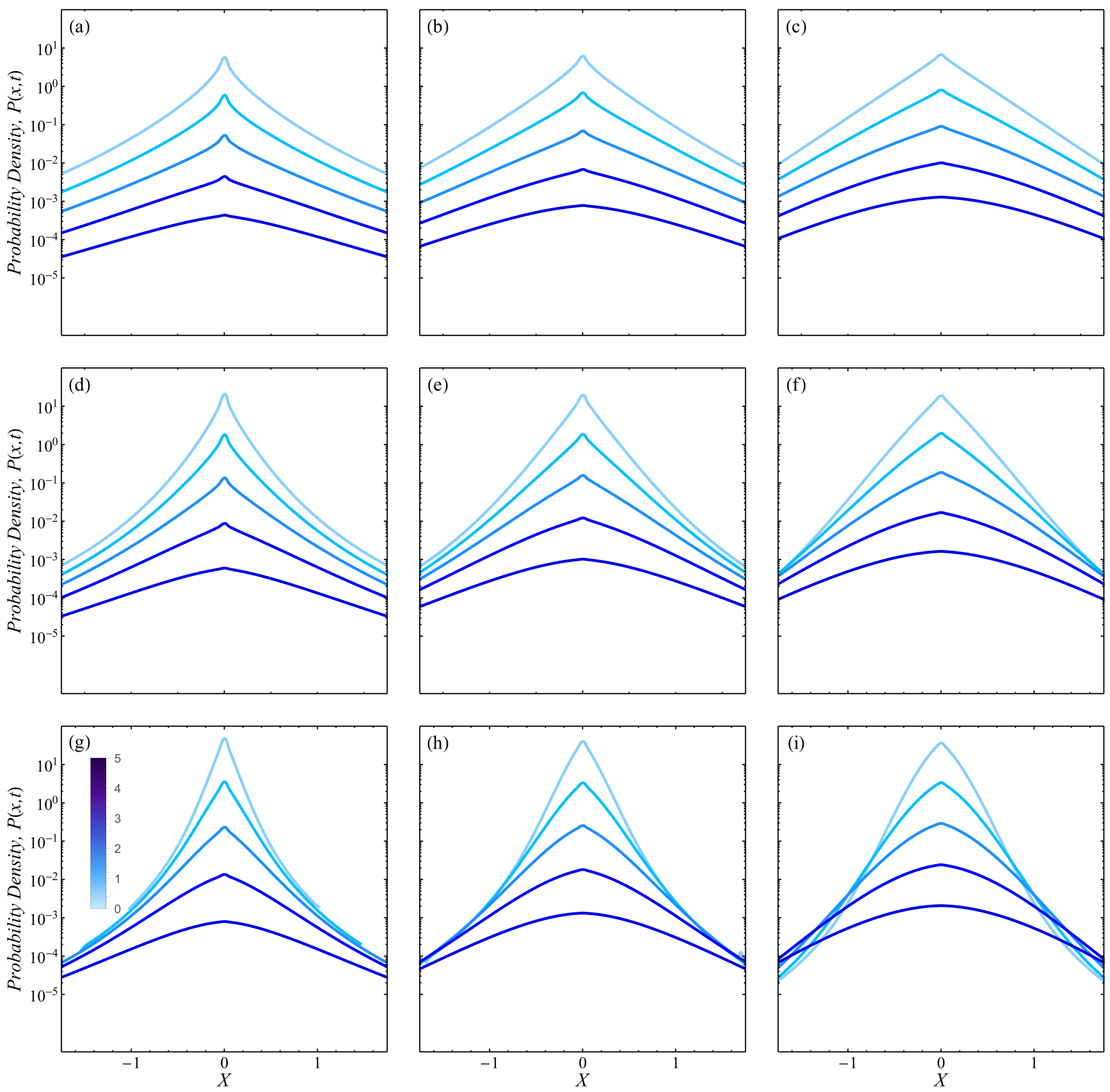
The solution $P(x,t)$ is contained within Figure 1 for a range of values of $\mu$ and $\gamma$. It is of note that, through the methods of solution adopted in this article, the spatial parameter $\mu$ may have its range of values extended to $\mu \in (0,2]$, however the additional constraint that $\mu \ne \gamma$ is present if $\mu \in (0,1]$.

3.2.2. Normalisation

The normalisation of Equation (29) can be demonstrated using the Mellin transform, as shown before in the work of Sandev et al. [28]. After the evaluation of the Mellin transform, Equation (29) becomes,

$${\int }_0^{t}exp\left(-\frac{t^{\prime }}{\tau }\right)\sum _{m=0}^{\infty }\frac{1}{\mathsf{\Gamma }\left(m+1\right)}{\left(\frac{t^{\prime \gamma }}{{\tau }^{\gamma }}\right)}^m\frac{1}{t^{\prime }}\frac{1}{\mathsf{\Gamma }\left(\gamma m\right)\mathsf{\Gamma }\left(1-m\right)}d{t}^{\prime }.$$

(31)

Equation (31) has an equivalent form in terms of the Fox H function, after expressing it in this manner and taking the Laplace transform reveals

$$\frac{1}{u}{H}_{2,2}^{1,1}\left[-\frac{1}{{\left(u+\tau \right)}^{\gamma }{\tau }^{\gamma }}{|}_{(0,1),(1,\gamma )}^{(1,\gamma )(1,1)}\right]=\frac{1}{u}{\left(1+\frac{1}{{\left(u+\tau \right)}^{\gamma }{\tau }^{\gamma }}\right)}^0=\frac{1}{u}$$

(32)

3.2.3. Reduction $\gamma \to 1$

If $\gamma \to 1$, Equation (29) should reduce to the standard Lévy solution. The first step is to remove the factor ${(-1)}^m$ from the Fox H function followed by taking the factor $(-1)$ into the Fox H function, both via the relations discussed in Skibinski et al. [29]

$$P(x,t)=\frac{1}{\sqrt{\pi }}{\int }_0^t\frac{(-1)}{t^{\prime }\left|x\right|}{H}_{1,2}^{1,1}\left[\frac{{\tau }^{\gamma }{\left|x\right|}^{\mu }}{2^{\mu }{\sigma }^{\mu }{t}^{\prime }}{|}_{(\frac{1}{2},\frac{\mu }{2})(1,\frac{\mu }{2})}^{(0,1)}\right].$$

(33)

Laplace transforming this to resolve the integral, provides the following expression for $P(x,u)$

$$P(x,u)=\frac{1}{\sqrt{\pi }}\frac{(-1)}{u\left|x\right|}{H}_{1,3}^{2,1}\left[\frac{{\tau }^{\gamma }{\left|x\right|}^{\mu }u}{2^{\mu }{\sigma }^{\mu }}{|}_{(0,1)(\frac{1}{2},\frac{\mu }{2})(1,\frac{\mu }{2})}^{(0,1)}\right].$$

(34)

The inversion of this followed by bringing the factor $(-1)$ back into the H function, enables the cancellation of the coefficient pair $(0,1)$.

$$P(x,t)=\frac{1}{\sqrt{\pi }}\frac{1}{\left|x\right|}{H}_{1,2}^{1,1}\left[\frac{{\tau }^{\gamma }{\left|x\right|}^{\mu }}{2^{\mu }{\sigma }^{\mu }t}{|}_{(\frac{1}{2},\frac{\mu }{2})(1,\frac{\mu }{2})}^{(1,1)}\right].$$

(35)

From this expression you may simply remove $\mu$ from the Fox H function (see known properties [30]), insert a symmetric coefficient pair $(1,\frac{1}{2})$ followed by the employment of the Legendre duplication formula on the coefficient pairs $(1,\frac{1}{2})$ and $(\frac{1}{2},\frac{1}{2})$ to complete the extraction of the standard Lévy form, as required [11].

$$P(x,t)=\frac{1}{\left|x\right|\mu }{H}_{2,2}^{1,1}\left[\frac{\tau \left|x\right|}{\sigma t^{\frac{1}{\mu }}}{|}_{(1,1)(1,\frac{1}{2})}^{(1,\frac{1}{\mu })(1,\frac{1}{2})}\right].$$

(36)

3.2.4. Reduction $\mu \to 2$

If $\mu \to 2$ the Gaussian propagator should be recovered and that is now demonstrated. Starting from Equation (29) we set $\mu \to 2$, which gives,

$$P(x,t)=\frac{1}{\sqrt{\pi }}{\int }_0^{t}exp\left(-\frac{t^{\prime }}{\tau }\right)\sum _{m=0}^{\infty }\frac{1}{\mathsf{\Gamma }\left(m+1\right)}{\left(-\frac{t^{\prime \gamma }}{{\tau }^{\gamma }}\right)}^m\frac{1}{t^{\prime }\left|x\right|}{H}_{3,4}^{2,2}\left[\frac{{\tau }^{\gamma }{x}^2}{4{\sigma }^2{t}^{\prime \gamma }}{|}_{(\frac{1}{2},1)(1,1)(1,1)(m,1)}^{(1,1)(0,1)(\gamma m,\gamma )}\right]d{t}^{\prime }.$$

(37)

We then combine coefficients by way of the Legendre duplication relation, and then reduce the H function to give,

$$P(x,t)=\frac{1}{2}{\int }_0^{t}exp\left(-\frac{t^{\prime }}{\tau }\right)\sum _{m=0}^{\infty }\frac{1}{\mathsf{\Gamma }\left(m+1\right)}{\left(\frac{t^{\prime \gamma }}{{\tau }^{\gamma }}\right)}^m\frac{1}{t^{\prime }\left|x\right|}{H}_{2,2}^{1,1}\left[\frac{{\tau }^{\frac{\gamma }{2}}\left|x\right|}{\sigma t^{\prime \frac{\gamma }{2}}}{|}_{(1,1)(m,\frac{1}{2})}^{(0,\frac{1}{2})(\gamma m,\frac{\gamma }{2})}\right]d{t}^{\prime }.$$

(38)

This is the integral form identified for the Gaussian CTRW case, as required.

3.2.5. Short Timescale Asymptotics

In the very small t regime, such that $exp\left(-\frac{t}{\tau }\right)\approx 1$, and the dominant term of the series over m is $m=0$, in which case the solution to Equation (29) reduces to the following integral form,

$$\begin{array}{cc}\hfill P(x,t)& =\frac{1}{\sqrt{\pi }}{\int }_0^t\frac{1}{t^{\prime }\left|x\right|}{H}_{2,3}^{2,1}\left[\frac{{\tau }^{\gamma }{\left|x\right|}^{\mu }}{2^{\mu }{\sigma }^{\mu }{t}^{\prime \gamma }}{|}_{(\frac{1}{2},\frac{\mu }{2})(1,1)(1,\frac{\mu }{2})}^{(1,1)(0,\gamma )}\right]d{t}^{\prime }\hfill \\ & =\frac{1}{\sqrt{\pi }}\frac{1}{\left|x\right|}{H}_{2,3}^{2,1}\left[\frac{{\tau }^{\gamma }{\left|x\right|}^{\mu }}{2^{\mu }{\sigma }^{\mu }{t}^{\gamma }}{|}_{(\frac{1}{2},\frac{\mu }{2})(1,1)(1,\frac{\mu }{2})}^{(1,1)(1,\gamma )}\right].\hfill \end{array}$$

(39)

Which is the solution to the Riemann–Liouville space-time fractional diffusion equation.

3.2.6. Long Timescale Asymptotics

In order to explore the long timescale asymptotic behaviour, the first step is to remove the factor ${(-1)}^m$ by way of property 3.5 of the work of Skibinski [29]. Following this, the Fox H function may be expressed in the series form as described in brief in the article of Metzler et al. [31] and in detail in the landmark text by Saxena and Mathai [27]. The series form contains a nested pair of summations, one between 0 and ∞ and the other from 1 to 3. The latter has only one non-zero component (corresponding to the coefficient pair $(\frac{1}{2},\frac{\mu }{2})$) which we now outline,

$$\begin{array}{ll}\frac{1}{t\left|x\right|}{H}_{3,4}^{2,2}\left[\frac{{\tau }^{\gamma }{\left|x\right|}^{\mu }}{2^{\mu }{\sigma }^{\mu }{t}^{\gamma }}{|}_{(\frac{1}{2},\frac{\mu }{2})(1,1)(1,\frac{\mu }{2})(m,1)}^{(1,1)(0,1)(\gamma m,\gamma )}\right]=\frac{1}{t\left|x\right|}\sum _{n=0}^{\infty }{\left(\frac{{\tau }^{\gamma }{\left|x\right|}^{\mu }}{2^{\mu }{\sigma }^{\mu }{t}^{\gamma }}\right)}^{\left(\frac{1}{2}+n\right)\frac{2}{\mu }}\frac{2}{\mu }& \hspace{1em}\hspace{1em}\hspace{1em}\hspace{1em}\hspace{1em}\hspace{1em}\hspace{1em}\hspace{1em}\hspace{1em}\hspace{1em}\hspace{1em}\hspace{1em}\hspace{1em}\hspace{1em}\end{array}$$

$$\begin{array}{c}\hfill \hspace{1em}\hspace{1em}\hspace{1em}\hspace{1em}\frac{\mathsf{\Gamma }\left(m-\frac{2}{\mu }\left(\frac{1}{2}+n\right)\right)\mathsf{\Gamma }\left(1-\frac{2}{\mu }\left(\frac{1}{2}+n\right)\right)\mathsf{\Gamma }\left(\frac{2}{\mu }\left(\frac{1}{2}+n\right)\right)}{\mathsf{\Gamma }\left(-\frac{2\gamma }{\mu }\left(\frac{1}{2}+n\right)\right)\mathsf{\Gamma }\left(\gamma m-\frac{2\gamma }{\mu }\left(\frac{1}{2}+n\right)\right)\mathsf{\Gamma }\left(\frac{1}{2}+n\right)\mathsf{\Gamma }\left(n+1\right)}.\end{array}$$

(40)

Reinserting Equation (40) into Equation (29), then collecting the series over m and expressing this as an H function, yields

$$\begin{array}{cc}\hfill P(x,t)& =\frac{1}{\sqrt{\pi }}{\int }_0^{t}exp\left(-\frac{t^{\prime }}{\tau }\right)\frac{1}{t\left|x\right|}\sum _{n=0}^{\infty }{\left(\frac{{\tau }^{\gamma }{\left|x\right|}^{\mu }}{2^{\mu }{\sigma }^{\mu }{t}^{\gamma }}\right)}^{\left(\frac{1}{2}+n\right)\frac{2}{\mu }}\frac{2}{\mu }\hfill \end{array}$$

$$\begin{array}{c}\hfill \hspace{1em}\hspace{1em}\hspace{1em}\hspace{1em}\hspace{1em}\hspace{1em}\hspace{1em}\hspace{1em}\frac{\mathsf{\Gamma }\left(\frac{2}{\mu }\left(\frac{1}{2}+n\right)\right)\mathsf{\Gamma }\left(1-\frac{2}{\mu }\left(\frac{1}{2}+n\right)\right)}{\mathsf{\Gamma }\left(-\frac{2\gamma }{\mu }\left(\frac{1}{2}+n\right)\right)\mathsf{\Gamma }\left(\frac{1}{2}+n\right)\mathsf{\Gamma }\left(n+1\right)}{H}_{1,2}^{1,1}\left[-\frac{t^{\gamma }}{{\tau }^{\gamma }}{|}_{(0,1)(1+\frac{2\gamma }{\mu }\left(\frac{1}{2}+n\right),\gamma )}^{(1+\frac{2}{\mu }\left(\frac{1}{2}+n\right),1)}\right]d{t}^{\prime }.\end{array}$$

(41)

The Fox H function contained in Equation (41) is able to be connected with the Wright function and this allows asymptotic behaviour to be readily extracted via the work of Wright [32]. Using the relationships identified by Wright, the following form can be extracted (using theorem 1 within, and the integer $M=1$)

$$\begin{array}{cc}\hfill P(x,t)& =\frac{1}{\sqrt{\pi }}{\int }_0^{t}exp\left(-\frac{t^{\prime }}{\tau }\right)\frac{1}{t\left|x\right|}\sum _{n=0}^{\infty }{\left(\frac{{\tau }^{\gamma }{\left|x\right|}^{\mu }}{2^{\mu }{\sigma }^{\mu }{t}^{\gamma }}\right)}^{\left(\frac{1}{2}+n\right)\frac{2}{\mu }}\frac{2}{\mu }\hfill \end{array}$$

$$\begin{array}{c}\hfill \hspace{1em}\hspace{1em}\hspace{1em}\hspace{1em}\hspace{1em}\hspace{1em}\hspace{1em}\hspace{1em}\hspace{1em}\hspace{1em}\hspace{1em}\hspace{1em}\frac{\mathsf{\Gamma }\left(\frac{2}{\mu }\left(\frac{1}{2}+n\right)\right)\mathsf{\Gamma }\left(1-\frac{2}{\mu }\left(\frac{1}{2}+n\right)\right)}{\mathsf{\Gamma }\left(-\frac{2\gamma }{\mu }\left(\frac{1}{2}+n\right)\right)\mathsf{\Gamma }\left(\frac{1}{2}+n\right)\mathsf{\Gamma }\left(n+1\right)}{\left(\frac{t}{\tau }\right)}^{(\gamma -1)\frac{2}{\mu }\left(\frac{1}{2}+n\right)}{\gamma }^{\frac{2}{\mu }\left(\frac{1}{2}+n\right)}exp\left(\frac{t}{\tau }\right)d{t}^{\prime }.\end{array}$$

(42)

After simplifying Equation (42) it may be recombined into the following H function expression

$$\begin{array}{cc}\hfill P(x,t)& =\frac{1}{\sqrt{\pi }}{\int }_0^t\frac{1}{t^{\prime }\left|x\right|}{H}_{2,3}^{2,1}\left[\frac{{\tau \left|x\right|}^{\mu }}{2^{\mu }{\sigma }^{\mu }{t}^{\prime }}{|}_{(\frac{1}{2},\frac{\mu }{2})(1,1)(1,\frac{\mu }{2})}^{(1,1)(0,1)}\right]d{t}^{\prime }\hfill \\ & =\frac{1}{\sqrt{\pi }}\frac{1}{\left|x\right|}{H}_{1,2}^{2,0}\left[\frac{{\gamma \tau \left|x\right|}^{\mu }}{2^{\mu }{\sigma }^{\mu }t}{|}_{(\frac{1}{2},\frac{\mu }{2})(1,\frac{\mu }{2})}^{(1,1)}\right]\hfill \\ & =\frac{1}{\sqrt{\pi }}\frac{1}{\left|x\right|}{H}_{2,3}^{2,1}\left[\frac{{\gamma \tau \left|x\right|}^{\mu }}{2^{\mu }{\sigma }^{\mu }t}{|}_{(1,\frac{\mu }{2})(\frac{1}{2},\frac{\mu }{2})(1,\frac{\mu }{2})}^{(1,1)(1,\frac{\mu }{2})}\right]\hfill \\ & =\frac{1}{\sqrt{\pi }}\frac{1}{\left|x\right|}{H}_{2,2}^{1,1}\left[\frac{{\gamma \tau \left|x\right|}^{\mu }}{{\sigma }^{\mu }t}{|}_{(1,\mu )(1,\frac{\mu }{2})}^{(1,1)(1,\frac{\mu }{2})}\right].\hfill \end{array}$$

(43)

To summarise the steps involved in Equation (43), the integral is first evaluated after a reduction is afforded due to the symmetry of the coefficients. The symmetric coefficients $(1,\frac{\mu }{2})$ are then inserted to allow the Legendre duplication formula to be used to combine the coefficient pair $(1,\frac{\mu }{2})(\frac{1}{2},\frac{\mu }{2})$. Thus it can be seen that for sufficiently large timescales the standard Lévy form is recovered. It is of note, however, that the anomalous exponent $\gamma$ remains present. It represents a lingering signature of the subdiffusive behaviour that was present on shorter timescales, which is analogous to the observations made in the work of Cleland and Williams [11] for long timescales.

4. Discussion and Conclusions

This research is concerned with developing a generalised diffusion equation capable of describing diffusion processes driven by underlying stress-redistributing (SR) type events. Previous work [11] has explored the resulting diffusion equation in the instance that only the timing of these SR jump-inducing events is considered. However, the present research incorporates spatial implications as well, encoded within the chosen displacement PDF in the underlying CTRW. The encoding was introduced via a Lévy stable PDF exhibiting the inverse power law tails also observed in SR models [22]. The resulting generalised diffusion equation was found in the so called hydrodynamic limit, which corresponds to the small k regime in the Fourier space, and its memory kernel was extracted. Its structure is different from that which was studied in Ref. [11] with regard to the spatial derivative, which is now fractional. The implications of a fractional derivative were explored in Section 3.1.1, within the context of the flow of probability current. The non-local nature of these derivatives was also demonstrated in Section 3.1.1, as the flow of PDC was determined to be directed down a non-local gradient. Section 3.2 then delved into the solution to the generalised diffusion equation discussed within this article. In obtaining the solution to Equation (12) via its Fourier and Laplace form, a small detour was taken to highlight a new subordinator connection to the standard Lévy PDF. This subordinator form mirrored extremely closely the form highlighted by Checkin et al. and Sokolov [24,25], however, differing slightly in the inclusion of the standard Lévy PDF. After this brief detour, the derivation of the solution to Equation (12) continued. Several relations closely connected with the Fox H function were exploited in the determination of the final PDF form, which is given in Equation (29) and shown in Figure 1. The employment of these Fox H function properties is something that has become an important tool in the study of fractional derivative equations in recent years [11,28,33,34]. Section 3.2.2–Section 3.2.4 deal with important behaviours that any solution of Equation (12) would be expected to have, confirming its validity. Specifically, in Section 3.2.2 the normalisation condition was confirmed, ensuring that $P(x,t)$ is a PDF. Section 3.2.3 demonstrated that in the instance $\gamma \to 1$$P(x,t)$ relaxed back to the standard Lévy PDF. Finally, Section 3.2.4 outlined the nature of the reduction back to the PDF described in the work of Cleland and Williams [11], upon the occurrence of $\mu \to 2$. This work represents the first time both spatial and temporal features of stress-redistribution driven diffusion have been encoded within a generalised diffusion equation. It is hoped that the analytic features outlined within this work will be of great use in the modelling of systems demonstrating diffusion driven by these stick-slip dynamics.

References

- Yin, Q.Q.; Li, Y.Y.; Marchesoni, F.; Nayak, S.; Ghosh, P.K. Non-Gaussian normal diffusion in low dimensional systems. Front. Phys. 2021, 16, 1–14. [Google Scholar] [CrossRef]
- Abe, S. Fokker-Planck approach to non-Gaussian normal diffusion: Hierarchical dynamics for diffusing diffusivity. Phys. Rev. E 2020, 102, 042136. [Google Scholar] [CrossRef] [PubMed]
- Gu, Q.; Schiff, E.A.; Grebner, S.; Wang, F.; Schwarz, R. Non-Gaussian transport measurements and the Einstein relation in amorphous silicon. Phys. Rev. Lett. 1996, 76, 3196–3199. [Google Scholar] [CrossRef] [PubMed]
- Scher, H.; Shlesinger, M.F.; Bendler, J.T. Time-scale invariance in transport and relaxation. Phys. Today 1991, 44, 26–34. [Google Scholar] [CrossRef]
- Klammler, F.; Kimmich, R. Geometrical restrictions of incoherent transport of water by diffusion in protein of silica fineparticle systems and by flow in a sponge—A study of anomalous properties using an nmr field-gradient technique. Croat. Chem. Acta 1992, 65, 455–470. [Google Scholar]
- Schaufler, S.; Schleich, W.P.; Yakovlev, V.P. Keyhole look at Lévy flights in subrecoil laser cooling. Phys. Rev. Lett. 1999, 83, 3162–3165. [Google Scholar] [CrossRef]
- Schaufler, S.; Schleich, W.P.; Yakovlev, V.P. Scaling and asymptotic laws in subrecoil laser cooling. Europhys. Lett. 1997, 39, 383–388. [Google Scholar] [CrossRef]
- Balescu, R. Anomalous transport in turbulent plasmas and continuous-time random-walks. Phys. Rev. E 1995, 51, 4807–4822. [Google Scholar] [CrossRef]
- Barkai, E.; Silbey, R. Diffusion of tagged particle in an exclusion process. Phys. Rev. E 2010, 81, 041129. [Google Scholar] [CrossRef]
- Fokker, A.D. The median energy of rotating electrical dipoles in radiation fields. Ann. der Phys. 1914, 43, 810–820. [Google Scholar] [CrossRef]
- Cleland, J.; Williams, M.A.K. Anomalous diffusion driven by the redistribution of internal stresses. Phys. Rev. E 2021, 104, 014123. [Google Scholar] [CrossRef]
- Montroll, E.W.; Weiss, G.H. Random walks on lattices. II. J. Math. Phys. 1965, 6, 167–181. [Google Scholar] [CrossRef]
- Klafter, J.; Sokolov, I. First Steps in Random Walks. From Tools to Applications; OUP Oxford: Oxford, UK, 2011. [Google Scholar]
- Shlesinger, M.F. Origins and applications of the Montroll-Weiss continuous time random walk. Eur. Phys. J. B 2017, 90, 1–5. [Google Scholar] [CrossRef]
- Metzler, R.; Klafter, J. The random walk’s guide to anomalous diffusion: A fractional dynamics approach. Phys. Rep.-Rev. Sect. Phys. Lett. 2000, 339, 1–77. [Google Scholar] [CrossRef]
- Vivirschi, B.N.; Boboc, P.C.; Baran, V.; Nicolin, A.I. Scale-free distributions of waiting times for earthquakes. Phys. Scr. 2020, 95, 044011. [Google Scholar] [CrossRef]
- Bialecki, M. On mechanistic explanation of the shape of the universal curve of earthquake recurrence time distributions. Acta Geophys. 2015, 63, 1205–1215. [Google Scholar] [CrossRef]
- Povstenko, Y. Linear Fractional Diffusion-Wave Equation for Scientists and Engineers; Springer: Cham, Switzerland, 2015. [Google Scholar] [CrossRef]
- Samko, S.G.; Kilbas, A.A.; Marichev, O.I. Fractional integrals and derivatives: Theory and applications. Teor. Mater. Fiz 1993, 3, 397–414. [Google Scholar]
- Kilbas, A.; Srivastava, H.; Trujillo, J. Theory and Applications Of Fractinal Differential Equations; Elsevier: Amsterdam, The Netherlands, 2006; Volume 204. [Google Scholar] [CrossRef]
- Podlubny, I. (Ed.) Chapter 2—Fractional derivatives and integrals. In Fractional Differential Equations; Mathematics in Science and Engineering; Elsevier: Amsterdam, The Netherlands, 1999; Volume 198, pp. 41–119. [Google Scholar] [CrossRef]
- Pica Ciamarra, M.; Lippiello, E.; De Arcangelis, L.; Godano, C. Statistics of slipping event sizes in granular seismic fault models. EPL (Europhys. Lett.) 2011, 95, 54002. [Google Scholar] [CrossRef]
- Fox, C. The g and h functions as symmetrical fourier kernels. Trans. Am. Math. Soc. 1961, 98, 395–429. [Google Scholar]
- Chechkin, A.V.; Sokolov, I.M. Relation between generalized diffusion equations and subordination schemes. Phys. Rev. E 2021, 103, 032133. [Google Scholar] [CrossRef]
- Sokolov, I.M. Solutions of a class of non-Markovian fokker-Planck equations. Phys. Rev. E 2002, 66 Pt 1, 041101. [Google Scholar] [CrossRef] [PubMed]
- Tateishi, A.A.; Ribeiro, H.V.; Lenzi, E.K. The role of fractional time-derivative operators on anomalous diffusion. Front. Phys. 2017, 5, 52. [Google Scholar] [CrossRef]
- Mathai, A.M.; Saxena, R.K. The H-Function with Applications in Statistics and Other Disciplines; John Wiley & Sons: Hoboken, NJ, USA, 1978. [Google Scholar]
- Sandev, T.; Chechkin, A.V.; Korabel, N.; Kantz, H.; Sokolov, I.M.; Metzler, R. Distributed-order diffusion equations and multifractality: Models and solutions. Phys. Rev. E 2015, 92, 042117. [Google Scholar] [CrossRef]
- Skibiński, P. Some expansion theorems for the H-function. Ann. Pol. Math. 1970, 23, 125–138. [Google Scholar] [CrossRef]
- Mathai, A.; Saxena, R.; Haubold, H. The H-Function: Theory and Applications; Springer: Berlin/Heidelberg, Germany, 2009. [Google Scholar] [CrossRef]
- Sandev, T.; Metzler, R.; Tomovski, Z. Fractional diffusion equation with a generalized Riemann-Liouville time fractional derivative. J. Phys. A Math. Theor. 2011, 44, 255203. [Google Scholar] [CrossRef]
- Wright, E.M. The asymptotic expansion of the generalized hypergeometric function. Proc. Lond. Math. Soc. 1940, s2-46, 389–408. [Google Scholar] [CrossRef]
- Langlands, T. Solution of a modified fractional diffusion equation. Appl. Anal. Acta. Phys. Pol. B 2003, 630, 259–279. [Google Scholar] [CrossRef]
- Awad, E.; Metzler, R. Crossover dynamics from superdiffusion to subdiffusion: Models and solutions. Fract. Calc. Appl. Anal. 2020, 23, 55–102. [Google Scholar] [CrossRef] [Green Version]
- Soury, H.; Alouini, M.S. On the symmetric alpha-stable distribution with application to symbol error rate calculations. In Proceedings of the 2016 IEEE 27th Annual International Symposium on Personal, Indoor, and Mobile Radio Communications (Pimrc), Valencia, Spain, 4–8 September 2016; pp. 990–995. [Google Scholar]
Figure 1.
Position probability density functions corresponding to increasing values of and in Equation (29), where X is dimensionless, . The value of ranges from (first row), to (third row), in increments of and ranges from (first column) to (third column) in increments of . The colours correspond to units of time, , within the open range (light blue to dark blue). These figures have used the values of and to be .
Publisher’s Note: MDPI stays neutral with regard to jurisdictional claims in published maps and institutional affiliations. |
© 2022 by the authors. Licensee MDPI, Basel, Switzerland. This article is an open access article distributed under the terms and conditions of the Creative Commons Attribution (CC BY) license (https://creativecommons.org/licenses/by/4.0/).
Share and Cite
MDPI and ACS Style
Cleland, J.D.; Williams, M.A.K. Analytical Investigations into Anomalous Diffusion Driven by Stress Redistribution Events: Consequences of Lévy Flights. Mathematics 2022, 10, 3235. https://0-doi-org.brum.beds.ac.uk/10.3390/math10183235
AMA Style
Cleland JD, Williams MAK. Analytical Investigations into Anomalous Diffusion Driven by Stress Redistribution Events: Consequences of Lévy Flights. Mathematics. 2022; 10(18):3235. https://0-doi-org.brum.beds.ac.uk/10.3390/math10183235
Chicago/Turabian StyleCleland, Josiah D., and Martin A. K. Williams. 2022. "Analytical Investigations into Anomalous Diffusion Driven by Stress Redistribution Events: Consequences of Lévy Flights" Mathematics 10, no. 18: 3235. https://0-doi-org.brum.beds.ac.uk/10.3390/math10183235
Note that from the first issue of 2016, this journal uses article numbers instead of page numbers. See further details here.