


STSM: Spatio-Temporal Shift Module for Efficient Action Recognition


1
Institute of Information Science, Beijing Jiaotong University, Beijing 100044, China
2
School of Computer and Information Technology, Beijing Jiaotong University, Beijing 100044, China
*
Author to whom correspondence should be addressed.
Mathematics 2022, 10(18), 3290; https://0-doi-org.brum.beds.ac.uk/10.3390/math10183290
Submission received: 31 July 2022
/
Revised: 4 September 2022
/
Accepted: 5 September 2022
/
Published: 10 September 2022
(This article belongs to the Topic Machine and Deep Learning)
Abstract
:The modeling, computational complexity, and accuracy of spatio-temporal models are the three major foci in the field of video action recognition. The traditional 2D convolution has low computational complexity, but it cannot capture the temporal relationships. Although the 3D convolution can obtain good performance, it is with both high computational complexity and a large number of parameters. In this paper, we propose a plug-and-play Spatio-Temporal Shift Module (STSM), which is a both effective and high-performance module. STSM can be easily inserted into other networks to increase or enhance the ability of the network to learn spatio-temporal features, effectively improving performance without increasing the number of parameters and computational complexity. In particular, when 2D CNNs and STSM are integrated, the new network may learn spatio-temporal features and outperform networks based on 3D convolutions. We revisit the shift operation from the perspective of matrix algebra, i.e., the spatio-temporal shift operation is a convolution operation with a sparse convolution kernel. Furthermore, we extensively evaluate the proposed module on Kinetics-400 and Something-Something V2 datasets. The experimental results show the effectiveness of the proposed STSM, and the proposed action recognition networks may also achieve state-of-the-art results on the two action recognition benchmarks.
1. Introduction
With the rapid development of camera equipment and mobile phones, video data has exploded in recent years. The massive amount of video information has far exceeded the processing power of traditional artificial systems, which has aroused people’s research interest in video understanding. As a fundamental task in video understanding, video action recognition has become one of the most active research topics, widely applied in video surveillance, video retrieval, social security, and other fields.
Recently, significant progress has been made in video action recognition based on deep convolutional networks [1,2,3,4,5,6,7,8]. Action recognition based on 3D convolution, such as C3D [9] and I3D [3], can most intuitively enable the network to learn spatio-temporal features. However, I3D learns spatio-temporal features at the cost of hundreds of GFLOPs. The use of 3D convolution will cause a large number of parameters and more computational complexity, which greatly limit the practicability of related methods.
In order to reduce the amount of parameters and computational complexity, some works [10,11,12] decompose the 3D convolution kernel into the space part (e.g., ) and the time part (e.g., ). However, in practice, they are still with more parameters and computational complexity than the corresponding 2D convolutions. The recent state-of-the-art model TSM [4] has achieved a good balance between complexity and performance. It abandons the traditional time convolution and learns time features by moving features along the time dimension using a shift operation with zero computational complexity and parameters. After fusing the convolution results, it is combined with the backbone of 2D CNNs to obtain the most advanced performance with a small amount of computational complexity and parameters. This motivates us to focus on designing a plug-and-play module with zero computational complexity and zero parameters that can effectively learn spatio-temporal features.
In this paper, we propose a plug-and-play Spatio-Temporal Shift Module (STSM), which is a general-purpose zero computation complexity and zero parameters module. It has both high efficiency and high performance at the same time. First, we design a spatio-temporal shift convolution, which is () tensors performing a shift operation to improve network performance. It captures spatio-temporal information from multiple perspectives using 1D shift operations in T, H, and W dimensions, enabling the network to learn spatio-temporal features in one, two, and even higher dimensions. Taking ResNet as an example, we add STSM before the first convolutional layer of each residual block. The feature tensor is divided by channel. Selected channels perform different shift operations to learn multi-view features, and the remaining channels remain unchanged. Then the final network is built by embedding STSM in each residual block. We have conducted extensive experiments on multiple well-known large datasets, including Kinetics-400 [13] and Something-Something V2 [14]. The experimental results fully demonstrate the effectiveness of our STSM. As shown in Figure 1, compared with existing state-of-the-art methods, our proposed STSM exhibits competitive performance on Something-Something V2. We achieve higher performance with less computation and less sampling. For Kinetics-400, STSM enhances the network accuracy without increasing the number of parameters and computational complexity.
The contributions of our paper are summarized as follows:
- We propose a plug-and-play Spatio-Temporal Shift Module (STSM), which is a module with zero computational complexity and parameters but powerful spatio-temporal modeling capabilities. A new perspective is proposed for efficient video model design by performing shift operations in different dimensions. Moreover, we revisit our spatio-temporal shift operation, which is essentially a convolution with a sparse convolution kernel, from the perspective of matrix algebra.
- Video action has strong spatio-temporal correlations, but action recognition models based on 2D CNNs backbone networks cannot effectively learn spatio-temporal features. To learn more spatio-temporal features at zero cost, we integrated the proposed STSM module in some typical 2D action recognition models in a plug-and-play fashion, such as TSN [2], TANet [16], and TDN [17] etc. Furthermore, our STSM combined with 2D action recognition models achieves higher performance than 3D action recognition models.
- Extensive experiments were conducted to verify the effectiveness of our method. Compared with existing methods, the proposed module achieves state-of-the-art or competitive results on the Kinetics-400 and Something-Something V2 datasets. Moreover, our STSM does not increase the computational complexity and parameters.
2. Related Work
2.1. 2D CNNs
2D CNNs were widely used in various fields of deep learning [18,19,20,21,22]. Inspired by the great success of deep convolution models in image recognition [21,23,24], many methods based on 2D CNNs have been proposed to apply deep learning for the field of video action recognition. In these methods, based on the two-stream architecture of 2D CNNs [1,25], video features could be learned from RGB streams and optical flow streams or motion vectors, respectively. Then, the outputs of the two streams were fused to obtain the prediction result. TSN [2] added a sparse time sampling strategy to the two-stream structure to further improve performance. TRN [15] used the multi-scale temporal relationship between sampled frames to improve model performance. Recently, GST [26], GSM [27], TEINet [28] focused on solving the problem of efficient time modeling. TSM [4] proposes a general plug-and-play temporal shift module with zero computational complexity and parameters. TSM enables 2D CNNs to learn temporal features without burden by simply shifting the feature tensor in memory along the temporal dimension. TEA [5] also designs small modules to enhance network performance. It designs temporal excitation and aggregation modules to capture network features’ short-term and long-term temporal evolution through feature differentiation and accumulation, respectively. TDN [17] used the time difference operator to design a module that can capture multi-scale time information to achieve effective action recognition. STM [29] learned spatio-temporal features and encoded motion features by designing spatio-temporal modules and motion modules on the channel, respectively.
2.2. 3D CNNs and (2+1)D CNNs Variants
Since 3D CNNs can learn good spatio-temporal features, they were widely used in the field of action recognition. C3D [9] was the first work to apply 3D CNNs to action recognition, which directly used 3D convolution to learn the spatio-temporal features of the video. However, C3D has too many parameters, which make it more difficult to be trained than 2D CNNs. I3D [3] initialized the network by inflating the 2D convolution pre-trained by ImageNet to 3D convolution, which improved the performance while reducing computation time. S3D [11], P3D [10], R(2+1)D [12], and StNet [30] were inspired by I3D, and could learn spatio-temporal features while reducing the computation complexity of 3D convolution. These (2+1)D CNNs resolved 3D convolutions into 2D spatial convolutions and 1D temporal convolutions. ECO [31] and ARTNet [32] combined 2D and 3D information in CNN blocks to enhance the network’s ability of learning features. Recently, SlowFast [33] explored the use of two different 3D CNN architectures to learn apparent features and motion features. TPN [6] adopted a plug-and-play universal time pyramid network at the feature level, which can be flexibly integrated into a 2D or 3D backbone network. Ref. [34] proposes methods for extracting semantic-aware visual attention and synthesizing fusion hierarchical semantic information to jointly interactively learn better features. ATFR [35] improved the energy efficiency of the network by introducing a differentiable Similarity Guided Sampling (SGS) module, and can be inserted into any existing 3D CNN architecture. ACTION-Net [8] designed a universal and effective module with 3D convolution and used it in 2D CNNs to enable the network to learn spatio-temporal features. CSTANet [36] designed a lightweight and efficient channel-wise spatio-temporal aggregation block that could be flexibly inserted into 2D CNNs. DSA-CNNs [37] effectively exploit the dense semantic information of videos by using bottom-up attention in the spatial flow and fusing the temporal flow. FEXNet [38] proposes a foreground extraction block to explicitly model foreground cues for effective management of action subjects. STFT [39] proposed a spatio-temporal short-term Fourier transform block that can replace 3D convolution.
3. Spatio-Temporal Shift Module (STSM)
The STSM is a plug-and-play module with zero computation complexity and parameters. It can effectively and efficiently encode spatio-temporal features after being embedded in the target network. In this section, we first introduce the details of our Spatio-Temporal Shift Module (STSM) and how to insert it into the existing architecture of CNN. Then we revisit that the essence of the shift operation in the STSM module is a convolution with a sparse convolution kernel from a matrix algebraic point of view.
3.1. Efficient Action Recognition based on STSM
Our STSM is a plug-and-play module that can be inserted into any convolutional layer of the network. Take the ResNet structured network for an exmaple, we insert the STSM module as shown in the red rounded rectangle in the middle of the Figure 2. Only one STSM module is inserted into each residual block, and the insertion position is before the first convolutional layer inside the residual block.
Figure 2 shows the network structure after embedding our STSM module in ResNet-50 [24]. The blue rounded rectangle at the bottom left is a schematic diagram of the structure of the STSM module. The green rounded rectangle in the lower right corner of Figure 2 is a schematic diagram of the 1D shift operation in the width dimension. The difference between time dimension shift, height dimension shift, and width dimension shift is the dimension of the shift operation, so we only introduce the width shift operation. Here we need to perform a shift operation on the tensor . We treat this tensor as a 3D tensor, where one dimension is the channel C, one dimension is the width W, and the other dimension is all the remaining dimensions. The leftmost part of the green rounded rectangle in the lower right corner of Figure 2 is the 3D coordinate system of the 1D width shift. The vertical axis is the channel dimension, the horizontal axis is the width dimension, and the third axis is the combined dimension of time and height. Divide the tensor into upper and lower halves along the channel dimension. The upper and lower halves of the tensor are shifted one bit to the left and one to the right, respectively, along the width dimension. The 1D spatio-temporal shift operation, time dimension (T) + height dimension (H) + width dimension (W), combined with subsequent convolutions allows the network to learn the results of 2D spatio-temporal shift operations and even 3D spatio-temporal shift operations.
The 2D spatio-temporal shift operation is to perform the shift operation on two dimensions in the same channel, respectively. Specifically, the 2D spatio-temporal shift operation is TH+TW+HW, where, TH represents the two-dimensional space formed by the time dimension and the height dimension, TW refers to the time and width dimensions, and HW refers to the height and width dimensions. The 3D spatio-temporal shift operation is to perform the shift operation on the three dimensions in the same channel, respectively. Therefore, the 3D spatio-temporal shift operation is THW, which represents the three-dimensional space formed by the time, height, and width dimensions. Applying shift operation only to the spatial dimension [40] or the time dimension [4] does not fully release the potential of the shift operation. Therefore, we propose a spatio-temporal shift operation to make the shift operation play a more significant role.
Because our 1D spatio-temporal shift operation cooperates with subsequent convolutions to obtain 1D, 2D and 3D spatio-temporal shift results, therefore, to enable the network to adaptively select 1D, 2D, and 3D spatio-temporal shift operation to learn spatio-temporal features based on samples, our STSM only uses 1D spatio-temporal shift operation based on time dimension + height dimension + width dimension (T+H+W). In contrast, TSM [4] only used 1D shift operations in the temporal dimension, and the network can only learn temporal and spatial features through shift and convolution, respectively. The specific verification will be given in detail in the ablation analysis in Section 5.1.2 later.
3.2. Spatio-Temporal Shift Operation
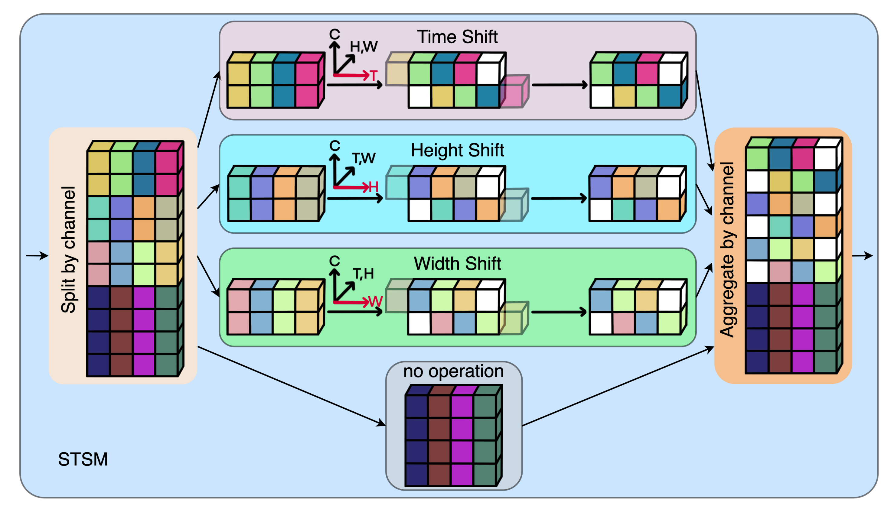
Our proposed STSM module using 1D spatio-temporal shift operation is shown in Figure 3. Our 1D spatio-temporal shift operation is divided into the following five steps:
- The feature tensor is divided into four parts by channel, where T, C, H, W represent the time, channel, height and width dimensions, respectively. Assume that is the ratio of the number of channels in the shift operation to the total number of channels, then , .
- For feature tensor after segmentation, it is divided into two parts and according to the channel. Then and are shifted forward and backward by one position in the time dimension to obtain the shifted tensors . Next, we concatenate and into along the channel dimension.
- For the second tensor and third feature tensor after segmentation, the same shift operation as the first feature tensor is performed in the height dimension and the width dimension, respectively. Then we get the 1D shifted tensors .
- The remaining feature tensor remains unchanged.
- Finally, we concatenate the above four feature tensors , , , and along the channel dimension to obtain a 1D spatio-temporal shifted tensor .
In this way, our 1D spatio-temporal shift operation is completed.
Figure 3.
Time (T) + height (H) + width (W) 1D Spatio-temporal shift operation.

The shift operation completes the special convolution operation by moving the position of the tensor without any calculation operation and does not need to store parameters at the same time. Specifically, the shift operation is equivalent to a convolution operation using a special sparse convolution kernel. This sparse convolution kernel has only one non-zero component with a value of 1. In order to ensure the high efficiency of the module, we try our best to make the shift operation corresponding to the sparse convolution kernel have the greatest change to the input matrix. Therefore, when the dimensions before and after the convolution are unchanged, the padding methods corresponding to different sparse convolution kernels are different. The specific method is to perform a padding operation on one side of the non-zero item. Assuming that the dimension of the sparse convolution kernel is , when and , the dimensional convolution kernel has only two combinations, i.e.:
Under the premise that the dimension of the matrix is unchanged, to complete the convolution operation of the above two convolution kernels, it is necessary to perform the zero-padding operation on the matrix. Corresponding to the above-mentioned convolution kernels and , we respectively add zeros in the rightmost column and the leftmost column of the feature matrix. The sparse convolution operation corresponding to the 1D spatio-temporal shift operation is shown in Figure 4. The shift operation corresponding to the convolution kernel is to shift the entire matrix by one column to the left. The specific operation is to delete the leftmost column of the input matrix, then add a column of all zero vectors to the rightmost column. The shift operation corresponding to the convolution kernel is opposite to the shift operation of the convolution kernel .
When and , the convolution kernel is:
The shift operation is similar to the dimensional convolution kernel, and the left and right shift of the matrix becomes the up and down shift.
When and , there are only four combinations of -dimensional convolution kernels, i.e.,:
The above-mentioned 2D convolution kernel is more complicated than the 1D convolution kernel. The shift corresponding to the 1D sparse convolution kernel only needs to move the matrix once. The 2D sparse convolution needs to move twice to complete the shift operation. Take the first sparse convolution kernel in Equation (3) as an example. In the case of the same input and output dimensions, complete the shift operation through the following steps:
- Delete the rightmost column of the input matrix and add a column of zero vectors to the leftmost column.
- Delete the bottom row of the matrix obtained in the previous step, and add a row of zero vectors to the top row.
The order of these two steps can be interchanged. In this way, the convolution operation of a special 2D sparse convolution kernel is completed without any calculation. Intuitively, it is equivalent to shifting the input matrix to the right one time and then to the bottom one time. Moreover, the 3D shift operation needs to move three times to complete.
4. Experimental Setting
This section introduces the experimental settings related to this paper. Bold in all tables represents the highest result.
4.1. Datasets and Evaluation Metrics
We evaluate our method on two large-scale datasets: Kinetics-400 (K400) [13] and Something-Something V2 (Sth-V2) [14]. Kinetics-400 has 400 human action categories, and the number of videos is approximately 240k training samples and 20k validation samples. For the Something-Something V2 dataset, the actions in it have a strong temporal relationship, so it is difficult to classify. It contains 220k videos, and the number of categories is 174 fine-grained categories.
We report the Top-1 accuracy (%) of Kinetics-400 and Something-Something V2. In addition, we use computational complexity (e.g., FLOPs or GFLOPs) and the number of model parameters to describe model complexity. If there are no special instructions, all use ImageNet for pre-training. #F and #Para indicate the number of frames and the number of parameters, respectively.
4.2. Implementation Details
Unless otherwise stated, all experiments were performed on MMAction2 [41] using RGB frames and evaluated on the validation set. The detailed setting and parameters of the proposed STSM module are designed as follows.
4.2.1. Training
The parameters for training on the Kinetics-400 are: 100 training epochs, initial learning rate (decays at epochs 40 and 80 by 0.1), batch size 48, and dropout 0.5. The entire network uses stochastic gradient descent (SGD) for end-to-end training, with a momentum of 0.9 and a weight decay of . The sample input strategy uses the built-in DenseSampleFrames type of MMAction2, where clip_len = 1, frame_interval = 1, num_clips = 8, aiming at the feature that the number of frames of a single video sample in the Something-Something V2 dataset is small. Therefore, the sample input strategy uses the built-in SampleFrames type of MMAction2, where clip_len = 1, frame_interval = 1, and num_clips = 8. The parameters for training on the Something-Something V2 are: 50 training epochs, initial learning rate (decays at epochs 20 and 40 by 0.1), batch size 48, and dropout 0.5. The shortest side of the input frame size will be pre-adjusted to 256 pixels, and then one of the ten-crops will be randomly used to crop the frame to . The ten-crops are top left, top right, center, bottom left, bottom right, and their horizontal mirroring flips.
4.2.2. Inference
The frame sampling setting during inference is the same as during training. After cropping the shortest side of the frame to 256 pixels, then uniformly cropping them into pixel frames, and finally averaging the output of three-crops to obtain the final output. Moreover, we set ten clips for Kinetics-400 clips and one clip for Something-Something V2, respectively.
5. Experimental Results
5.1. Ablation Analysis
5.1.1. Paramter Choice
Experiments in TSM [4] show that shifting the features on all channels is the best choice when performing the shift operation of the feature tensor. The reason is that too many original features are lost, so moving the features on only part of the channels is not an optimal choice. Therefore, we split the feature tensor of the current layer into parts according to the channel. We define the ratio of the number of channels of the shift operation to the total number of channels of the feature tensor as . For example, when , if the total number of channels at this time is 72, the shift operation is performed on the 1st to 18th channels, and the remaining 19th to 72th channels remain unchanged. Table 1 compares the performance of STSM under different . We use ImageNet pre-trained 2D ResNet-50 based TSN [2] as the backbone network and embed our STSM in it. At the same time, the shift dimension of STSM is set to T+H+W, i.e., we perform a one-dimensional shift operation in the time dimension, height dimension, and width dimension, respectively. The data in the table is the Top-1 accuracy rate (%) on the validation set of the Kinetics-400 dataset. The backbone of all networks is ResNet-50. GFLOPs in all tables are specified as GFLOPs×Crops×Clips. Unless otherwise stated, the inputs in all tables are RGB frames.
According to the results in Table 1, we can see that our STSM will have different performances under different settings. It can be observed that the performance reaches the highest point when . When , the accuracy will decrease as decreases. When , the accuracy will decrease with the increase of . This is equivalent to performing a shift operation on the first of the channels of the feature tensor, and the remaining channels remain unchanged. Because the shift dimension of STSM is set to T+H+W at this time, with a numerator of 3 will appear. For simplicity, we treat the levels of each dimension as equal. It is worth noting that our choice of is different from TSM () [4]. The in TSM is equivalent to setting in our STSM. In the best in our STSM experiment, we only perform shift operations along the time dimension on the first of the channel. In the subsequent experiments, unless otherwise specified, our is set to .
5.1.2. Different Shift Operations
Our STSM is a spatio-temporal shift convolution module, which can be 1D, 2D, or even higher-dimensional shift transformation. How to choose the right shift dimension is an important issue. Table 2 shows the network performance when we only add 1D and 2D shift convolutions in the spatial dimension. Table 3 shows the network performance when we add 1D and 2D shift convolutions to the spatio-temporal dimension.
As shown in Table 2, it can be seen that on 2D CNNs, the performance of the network using only spatial shift is improved compared with the backbone network TSN [2]. However, it is not as good as the network using only temporal shift. Therefore, this experiment demonstrates that temporal features are essential for 2D CNNs. At the same time, it is also proved that only the spatial shift operation is also effective. For video-based action tasks, compared with a pure spatial shift operation, adding a temporal shift operation to a 2D CNN enables the network to learn temporal features, which is a process from 0 to 1. Therefore, the performance boosted by only temporal shift is much better than that of only spatial shift. Among them, the network performance of adding a 1D spatial shift operation H and W is slightly higher than that of adding a 2D spatial shift operation HW. It is proved that after adding multiple 1D spatial shift operations to the network, the result after passing through the convolutional layer is equivalent to the result of adaptively selecting 1D, 2D, or higher-dimensional shift operations.
It can be seen from Table 3 that the performance of 2D CNNs with spatio-temporal shift is better than that of 2D CNNs with temporal shift only. The most basic 1D spatio-temporal shift combination has the best performance and the simplest shift operation required. Therefore, our STSM module chooses to use only the combination of Time shift + Height shift + Width shift (T+H+W). The performance of the 1D shift module with only T+H+W is slightly better than other spatio-temporal shift combinations. It can be seen that the 1D shift operation of T+H+W combined with the convolution operation can allow the network to adaptively select the required shift operations of different dimensions. Specifically, the network can utilize 1D shift (T, H, W) and subsequent convolutional layers to learn features with 2D shift (TH, TW, HW). In subsequent experiments, unless otherwise stated, our STSM only uses a one-dimensional shift operation, and the dimension of the shift operation is set to T+H+W. Since there are too many combinations of 3D shift, we did not do 3D shift research. However, experiments show that 1D shift outperforms 2D shift. It can be inferred that 3D shift is not as good as 1D shift.
5.2. Different Backbone
Our proposed STSM is a general-purpose plug-and-play module with no parameters and no additional operations. This experiment verifies that STSM can scale well to different backbone networks. Table 4 and Table 5 respectively show the results of our STSM after being embedded in different backbones on the validation sets of Kinetics-400 and Something-Something V2 datasets. In the experiment, ResNet-50 (R-50) [24] and MobileNetV2 (Mb_V2) [42] were used as the backbones. The methods in Table 4 have the same GFLOPs and parameters under the same backbone and input frames. In Table 5, the sampling method of our STSM is one clip, while the other methods are two clips. The input frame size of our STSM at inference is , while the other methods are . Therefore, our STSM is only of the computational complexity of TSM, although the backbone is the same and also has zero computational complexity and zero parameter modules. However, our STSM still outperforms them and leads by a large margin when the number of sampling frames is eight. Experimental results demonstrate that our STSM is a general plug-and-play module with zero computational complexity and zero parameters, which is effective under different backbone networks and input frame numbers.
5.3. Comparison with State-of-the-Arts
As a universal plug-and-play module with zero computation complexity and zero parameters, STSM significantly improves the 2D baseline. We embed our STSM into other models and compare them with state-of-the-art methods on the Kinetics-400 and Something-Something V2 datasets. When embedding our STSM into TDN [17], we replaced the TSM module in the original TDN with our STSM module.
5.3.1. Kinetics-400
Kinetics-400 is the current mainstream and challenging large-scale dataset. We compare the performance of STSM and the state-of-the-art method on the validation set of the Kinetics-400 dataset in the Table 6. Rfn152 refers to RefineNet [43] whose backbone network is ResNet-152 [24].
It can be seen from Table 6 that our STSM improves network performance more effectively than TSM without increasing the cost of computation complexity and the number of parameters. The network performance of our STSM embedded in 2D CNNs is also competitive with 3D CNNs. Especially compared with TPN [6], which also uses TSN [2] as the backbone, we have higher accuracy than TPN with 3D convolution when only 2D convolution is used. Compared with other networks based on 2D CNNs, our network can achieve higher performance with a lower amount of computation complexity and parameters. Compared with TSM [4], which is also based on TSN, our network has a higher accuracy rate. Compared with the original TSN, the accuracy of TSM with TSN as the backbone has increased by . The accuracy of our STSM with TSN as the backbone is increased by compared to the original TSN. Our STSM improves TSN by higher than TSM. Our STSM also improves the performance of networks with Non-local (NL) module [44], while X3D [45] can achieve good performance with low computational complexity and low amount of parameters. However, X3D is a well-designed network that is difficult to transfer to other networks, but our STSM can be easily plugged into other 2D CNN networks to boost performance. Moreover, X3D requires more input frames than eight to run. When a better performance 2D CNN-based action recognition network emerges in the future, inserting our STSM can achieve even better performance. Our STSM also achieves competitive results compared to TEA [5], TANet [16] and TDN [17]. We insert our STSM module into both TANet and TDN to improve the performance of the original network, demonstrating the effectiveness and plug-and-play properties of STSM. It should be noted that both TEA, TANet and TDN are specifically designed for ResNet [24], and our STSM can be easily embedded in other architectures, such as MobileNetV2 (Mb_V2) [42]. In particular, our STSM is a plug-and-play ultra-lightweight module with zero computation complexity and zero parameters. However, TEA, TANet and TDN are both complex modules that are with high computation complexity and parameters. Our STSM+TDN still outperforms the two-stream DSA-CNNs [37] based on 3D RefineNet (ResNet-152) [43] in the case of smaller computation and model volume.
5.3.2. Something-Something V2
Something-Something V2 is a challenging large dataset. Table 7 shows the performance comparison between our STSM and the state-of-the-art method under the validation set of the Something-Something V2 dataset. The video durations in the Something-Something V2 dataset are very short, but the spatio-temporal correlation of actions is higher. Because our STSM can learn better spatio-temporal features and model more complex spatio-temporal relationships, we obtain more competitive results than Kinetics-400 on the Something-Something V2.
Table 7 shows that our STSM consistently outperforms other methods under the same computational complexity. In models with less than 20G FLOPs of computational complexity, the backbone network at this time is 2D MobileNetV2. Our STSM performs better than TSM with the same computational complexity load of 15.36G FLOPs, and our STSM is still better than TSM with only 10.02G FLOPs of computational complexity. Our STSM improves the performance of TSM+NL. However, for our STSM, adding the NL module leads to performance degradation. This shows that for data with strong spatio-temporal correlation, our STSM can extract spatio-temporal features better than NL. When the number of input frames is eight, our STSM outperforms TSN by and TSM by , but at this time the computational complexity of our STSM is only of theirs. When the number of input frames is 16, the computational complexity of our STSM is only of that of TSM, and the performance of STSM is still higher than that of TSM. Under the same computational complexity, our STSM improves the performance of TANet from to . At this time, TANet adopts the same one-clip sampling strategy as ours. Our STSM also improves the performance of TDN. Our STSM+TDN is more accurate than FEXNet [38] with only of FEXNet’s GFLOPs. The effectiveness of our STSM is demonstrated.
5.4. Qualitative Results on Some Typical Samples
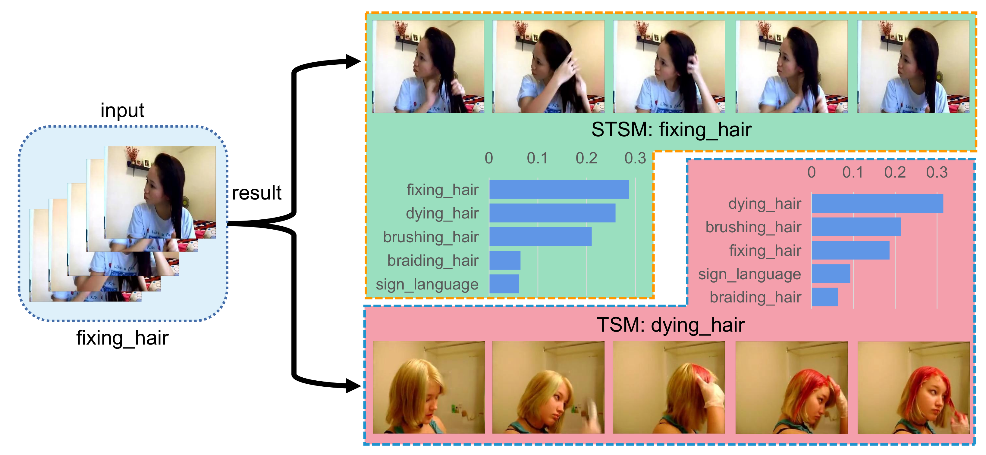
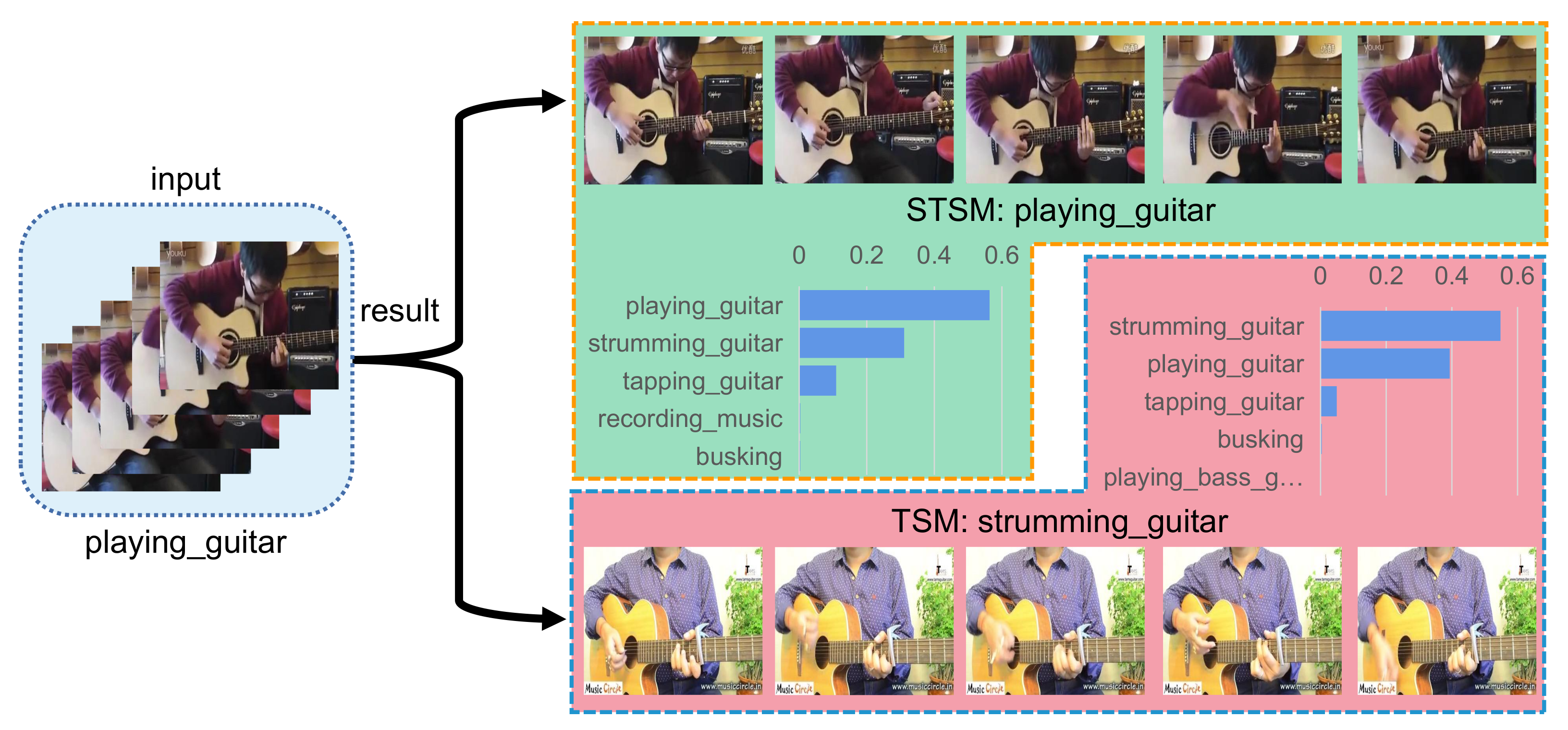
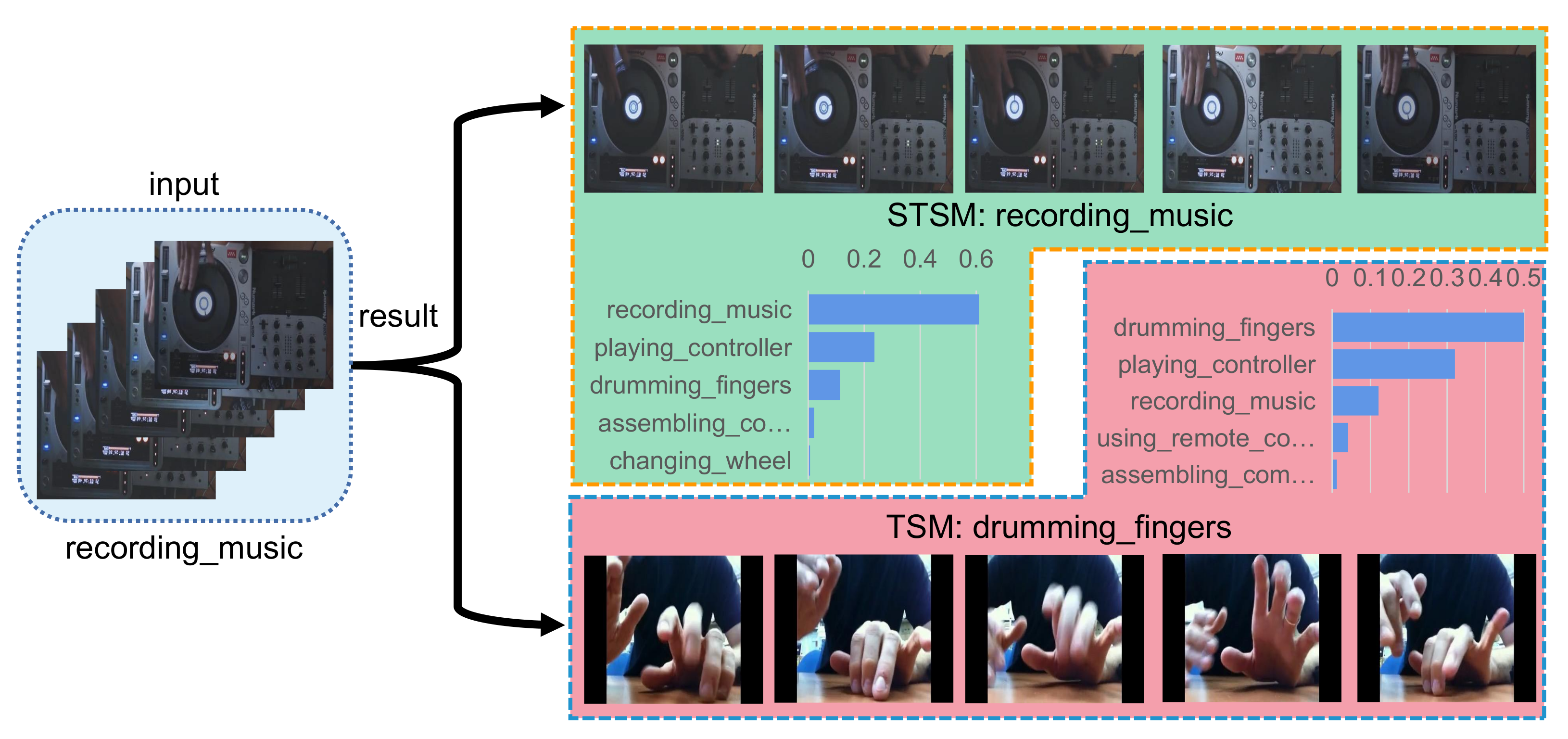
In this section, we select a few samples to visualize the experimental results. As shown in Figure 5, Figure 6 and Figure 7, we selected one sample from each of the three categories in the Kinetics-400 dataset for display. The three categories are fixing hair, playing guitar, and recording music, and our STSM is at least more accurate than TSM [4] in all three categories. The bar graph in the figure is the score graph of the top five of this sample. The horizontal axis is the score, and the vertical axis is the category. As can be seen from the figure, since our STSM can learn spatio-temporal features, TSM can only learn separate temporal features and temporal features. Therefore, our STSM can distinguish more different points in space and time to make the classification more accurate.
6. Conclusions
We propose a Spatio-Temporal Shift Module for efficient video recognition, which can be inserted into the network’s backbone in a plug-and-play manner to enhance network performance without increasing the amount of computation complexity and parameters. This module splits the feature tensor by channel and moves one position along the temporal and spatial dimensions, respectively, allowing the network to learn spatio-temporal features. Because STSM is essentially a special convolution with a sparse convolution kernel, it does not require extra calculation and no parameters. The action recognition model with STSM achieves state-of-the-art performance on the class-rich Kinetics-400 dataset and the motion-dominated Something-Something V2 dataset.
Author Contributions
Conceptualization, Z.Y. and G.A.; Data curation, Z.Y. and R.Z.; Formal analysis, Z.Y.; Methodology, Z.Y.; Supervision, G.A.; Writing—original draft, Z.Y.; Writing—review & editing, G.A. and R.Z. All authors have read and agreed to the published version of the manuscript.
Funding
This work was supported by the National Natural Science Foundation of China (62072028 and 61772067).
Institutional Review Board Statement
Not applicable.
Informed Consent Statement
Not applicable.
Data Availability Statement
Not applicable.
Conflicts of Interest
The authors declare no conflict of interest.
References
- Simonyan, K.; Zisserman, A. Two-Stream Convolutional Networks for Action Recognition in Videos. In Proceedings of the NIPS, Montreal, QC, Canada, 8–13 December 2014; pp. 568–576. [Google Scholar]
- Wang, L.; Xiong, Y.; Wang, Z.; Qiao, Y.; Lin, D.; Tang, X.; Gool, L.V. Temporal segment networks: Towards good practices for deep action recognition. In Proceedings of the ECCV, Amsterdam, The Netherlands, 8–16 December 2016. [Google Scholar]
- Carreira, J.; Zisserman, A. Quo Vadis, Action Recognition? A New Model and the Kinetics Dataset. In Proceedings of the CVPR, Honolulu, HI, USA, 21–26 July 2017. [Google Scholar]
- Lin, J.; Gan, C.; Han, S. TSM: Temporal Shift Module for Efficient Video Understanding. In Proceedings of the ICCV, Seoul, Korea, 27 October–2 November 2019. [Google Scholar]
- Li, Y.; Ji, B.; Shi, X.; Zhang, J.; Kang, B.; Wang, L. TEA: Temporal Excitation and Aggregation for Action Recognition. In Proceedings of the CVPR, virtually, 14–19 June 2020. [Google Scholar]
- Yang, C.; Xu, Y.; Shi, J.; Dai, B.; Zhou, B. Temporal Pyramid Network for Action Recognition. In Proceedings of the CVPR, virtually, 14–19 June 2020. [Google Scholar]
- Liu, X.; Pintea, S.L.; Nejadasl, F.K.; Booij, O.; van Gemert, J.C. No Frame Left Behind: Full Video Action Recognition. In Proceedings of the CVPR, virtually, 19–25 June 2021; pp. 14892–14901. [Google Scholar]
- Wang, Z.; She, Q.; Smolic, A. ACTION-Net: Multipath Excitation for Action Recognition. In Proceedings of the CVPR, virtually, 19–25 June 2021. [Google Scholar]
- Tran, D.; Bourdev, L.; Fergus, R.; Torresani, L.; Paluri, M. Learning Spatiotemporal Features With 3D Convolutional Networks. In Proceedings of the ICCV, Santiago, Chile, 13–16 December 2015. [Google Scholar]
- Qiu, Z.; Yao, T.; Mei, T. Learning Spatio-Temporal Representation with Pseudo-3D Residual Networks. In Proceedings of the ICCV, Venice, Italy, 22–29 October 2017. [Google Scholar]
- Xie, S.; Sun, C.; Huang, J.; Tu, Z.; Murphy, K. Rethinking spatiotemporal feature learning: Speed-accuracy trade-offs in video classification. In Proceedings of the ECCV, Munich, Germany, 8–14 September 2018. [Google Scholar]
- Tran, D.; Wang, H.; Torresani, L.; Ray, J.; LeCun, Y.; Paluri, M. A Closer Look at Spatiotemporal Convolutions for Action Recognition. In Proceedings of the CVPR, Salt Lake City, UT, USA, 18–22 June 2018. [Google Scholar]
- Kay, W.; Carreira, J.; Simonyan, K.; Zhang, B.; Hillier, C.; Vijayanarasimhan, S.; Viola, F.; Green, T.; Back, T.; Natsev, P.; et al. The Kinetics Human Action Video Dataset. arXiv 2017, arXiv:1705.06950. [Google Scholar]
- Goyal, R.; Ebrahimi Kahou, S.; Michalski, V.; Materzynska, J.; Westphal, S.; Kim, H.; Haenel, V.; Fruend, I.; Yianilos, P.; Mueller-Freitag, M.; et al. The “Something Something” Video Database for Learning and Evaluating Visual Common Sense. In Proceedings of the ICCV, Venice, Italy, 22–29 October 2017. [Google Scholar]
- Zhou, B.; Andonian, A.; Oliva, A.; Torralba, A. Temporal Relational Reasoning in Videos. In Proceedings of the ECCV, Munich, Germany, 8–14 September 2018; Ferrari, V., Hebert, M., Sminchisescu, C., Weiss, Y., Eds.; Lecture Notes in Computer Science; Springer: Berlin/Heidelberg, Germany, 2018; Volume 11205, pp. 831–846. [Google Scholar] [CrossRef]
- Liu, Z.; Wang, L.; Wu, W.; Qian, C.; Lu, T. TAM: Temporal Adaptive Module for Video Recognition. In Proceedings of the IEEE/CVF International Conference on Computer Vision (ICCV), virtually, 11–17 October 2021; pp. 13708–13718. [Google Scholar]
- Wang, L.; Tong, Z.; Ji, B.; Wu, G. TDN: Temporal Difference Networks for Efficient Action Recognition. In Proceedings of the CVPR, virtually, 19–25 June 2021. [Google Scholar]
- Krizhevsky, A.; Sutskever, I.; Hinton, G.E. ImageNet Classification with Deep Convolutional Neural Networks. In Proceedings of the NIPS, Lake Tahow, NV, USA, 3–6 December 2012; pp. 1106–1114. [Google Scholar]
- Girshick, R.B.; Donahue, J.; Darrell, T.; Malik, J. Rich Feature Hierarchies for Accurate Object Detection and Semantic Segmentation. In Proceedings of the CVPR, virtually, 19–25 June 2021; pp. 580–587. [Google Scholar] [CrossRef]
- Goodfellow, I.J.; Pouget-Abadie, J.; Mirza, M.; Xu, B.; Warde-Farley, D.; Ozair, S.; Courville, A.C.; Bengio, Y. Generative Adversarial Nets. In Proceedings of the NIPS, Montreal, QC, Canada, 8–13 December 2014; pp. 2672–2680. [Google Scholar]
- Simonyan, K.; Zisserman, A. Very Deep Convolutional Networks for Large-Scale Image Recognition. In Proceedings of the ICLR, San Diego, CA, USA, 7–9 May 2015. [Google Scholar]
- Redmon, J.; Divvala, S.K.; Girshick, R.B.; Farhadi, A. You Only Look Once: Unified, Real-Time Object Detection. In Proceedings of the CVPR, Las Vegas, NV, USA, 27–30 June 2016; pp. 779–788. [Google Scholar] [CrossRef]
- Ioffe, S.; Szegedy, C. Batch Normalization: Accelerating Deep Network Training by Reducing Internal Covariate Shift. In Proceedings of the ICML, Lille, France, 6–11 July 2015; Bach, F.R., Blei, D.M., Eds.; JMLR Workshop and Conference Proceedings; MLResearch Press: Singapore, 2015; Volume 37, pp. 448–456. [Google Scholar]
- He, K.; Zhang, X.; Ren, S.; Sun, J. Deep Residual Learning for Image Recognition. In Proceedings of the CVPR, Las Vegas, NV, USA, 27–30 June 2016. [Google Scholar]
- Zhang, B.; Wang, L.; Wang, Z.; Qiao, Y.; Wang, H. Real-Time Action Recognition with Enhanced Motion Vector CNNs. In Proceedings of the CVPR, Las Vegas, NV, USA, 27–30 June 2016; pp. 2718–2726. [Google Scholar] [CrossRef]
- Luo, C.; Yuille, A.L. Grouped Spatial-Temporal Aggregation for Efficient Action Recognition. In Proceedings of the ICCV, Seoul, Korea, 27 October–2 November 2019; pp. 5511–5520. [Google Scholar] [CrossRef]
- Sudhakaran, S.; Escalera, S.; Lanz, O. Gate-Shift Networks for Video Action Recognition. In Proceedings of the CVPR, virtually, 14–19 June 2020; pp. 1099–1108. [Google Scholar] [CrossRef]
- Liu, Z.; Luo, D.; Wang, Y.; Wang, L.; Tai, Y.; Wang, C.; Li, J.; Huang, F.; Lu, T. TEINet: Towards an Efficient Architecture for Video Recognition. In Proceedings of the AAAI, New York, NY, USA, 7–12 February 2020; pp. 11669–11676. [Google Scholar]
- Wang, M.; Xing, J.; Su, J.; Chen, J.; Yong, L. Learning SpatioTemporal and Motion Features in a Unified 2D Network for Action Recognition. IEEE Trans. Pattern Anal. Mach. Intell. 2022. [Google Scholar] [CrossRef] [PubMed]
- He, D.; Zhou, Z.; Gan, C.; Li, F.; Liu, X.; Li, Y.; Wang, L.; Wen, S. StNet: Local and Global Spatial-Temporal Modeling for Action Recognition. In Proceedings of the AAAI, Honolulu, HI, USA, 27 January–1 February 2019; pp. 8401–8408. [Google Scholar] [CrossRef]
- Zolfaghari, M.; Singh, K.; Brox, T. ECO: Efficient Convolutional Network for Online Video Understanding. In Proceedings of the ECCV, Munich, Germany, 8–14 September 2018; Lecture Notes in Computer Science. Springer: Berlin/Heidelberg, Germany, 2018; Volume 11206, pp. 713–730. [Google Scholar] [CrossRef]
- Wang, L.; Li, W.; Li, W.; Van Gool, L. Appearance-and-Relation Networks for Video Classification. In Proceedings of the CVPR, Salt Lake City, UT, USA, 18–22 June 2018. [Google Scholar]
- Feichtenhofer, C.; Fan, H.; Malik, J.; He, K. SlowFast Networks for Video Recognition. In Proceedings of the ICCV, Seoul, Korea, 27 October–2 November 2019; pp. 6201–6210. [Google Scholar] [CrossRef] [Green Version]
- Fu, J.; Gao, J.; Xu, C. Learning Semantic-Aware Spatial-Temporal Attention for Interpretable Action Recognition. IEEE Trans. Circuits Syst. Video Technol. 2021, 32, 5213–5224. [Google Scholar] [CrossRef]
- Fayyaz, M.; Bahrami, E.; Diba, A.; Noroozi, M.; Adeli, E.; Van Gool, L.; Gall, J. 3D CNNs With Adaptive Temporal Feature Resolutions. In Proceedings of the CVPR, virtually, 19–25 June 2021; pp. 4731–4740. [Google Scholar]
- Wang, H.; Xia, T.; Li, H.; Gu, X.; Lv, W.; Wang, Y. A Channel-Wise Spatial-Temporal Aggregation Network for Action Recognition. Mathematics 2021, 9, 3226. [Google Scholar] [CrossRef]
- Luo, H.; Lin, G.; Yao, Y.; Tang, Z.; Wu, Q.; Hua, X. Dense Semantics-Assisted Networks for Video Action Recognition. IEEE Trans. Circuits Syst. Video Technol. 2022, 32, 3073–3084. [Google Scholar] [CrossRef]
- Shen, Z.; Wu, X.J.; Xu, T. FEXNet: Foreground Extraction Network for Human Action Recognition. IEEE Trans. Circuits Syst. Video Technol. 2022, 32, 3141–3151. [Google Scholar] [CrossRef]
- Kumawat, S.; Verma, M.; Nakashima, Y.; Raman, S. Depthwise Spatio-Temporal STFT Convolutional Neural Networks for Human Action Recognition. IEEE Trans. Pattern Anal. Mach. Intell. 2022, 44, 4839–4851. [Google Scholar] [CrossRef] [PubMed]
- Wu, B.; Wan, A.; Yue, X.; Jin, P.; Zhao, S.; Golmant, N.; Gholaminejad, A.; Gonzalez, J.; Keutzer, K. Shift: A Zero FLOP, Zero Parameter Alternative to Spatial Convolutions. In Proceedings of the CVPR, Salt Lake City, UT, USA, 18–22 June 2018. [Google Scholar]
- Contributors, M. OpenMMLab’s Next Generation Video Understanding Toolbox and Benchmark. 2020. Available online: https://github.com/open-mmlab/mmaction2 (accessed on 30 July 2022).
- Sandler, M.; Howard, A.; Zhu, M.; Zhmoginov, A.; Chen, L.C. MobileNetV2: Inverted Residuals and Linear Bottlenecks. In Proceedings of the CVPR, Salt Lake City, UT, USA, 18–22 June 2018. [Google Scholar]
- Lin, G.; Milan, A.; Shen, C.; Reid, I. RefineNet: Multi-Path Refinement Networks for High-Resolution Semantic Segmentation. In Proceedings of the IEEE Conference on Computer Vision and Pattern Recognition (CVPR), Honolulu, HI, USA, 21–26 July 2017. [Google Scholar]
- Wang, X.; Girshick, R.B.; Gupta, A.; He, K. Non-local Neural Networks. arXiv 2017, arXiv:1711.07971. [Google Scholar]
- Feichtenhofer, C. X3D: Expanding Architectures for Efficient Video Recognition. In Proceedings of the IEEE/CVF Conference on Computer Vision and Pattern Recognition (CVPR), virtually, 14–19 June 2020. [Google Scholar]
- Li, X.; Wang, Y.; Zhou, Z.; Qiao, Y. SmallBigNet: Integrating Core and Contextual Views for Video Classification. In Proceedings of the CVPR, virtually, 14–19 June 2020. [Google Scholar]
- Zhi, Y.; Tong, Z.; Wang, L.; Wu, G. MGSampler: An Explainable Sampling Strategy for Video Action Recognition. In Proceedings of the ICCV, virtually, 11–17 October 2021; pp. 1513–1522. [Google Scholar]
Figure 1.
Video action recognition performance comparison in terms of Top-1 accuracy, computational complexity, and model size on the Something-Something V2 [14] dataset. Our STSM achieves higher accuracy with less computational complexity and number of parameters than TSM [4], TRN [15] and TSN [2].

Figure 2.
Network structure diagram after embedding STSM in ResNet-50. The convolutions are all 2D spatial convolutions, the first pooling layer is spatial max pooling, and the last pooling layer is an average time pooling. For simplicity, we did not draw the batch normalization layer and the activation function Relu in the figure.

Figure 4.
Revisiting of the 1D spatio-temporal shift operation from the perspective of matrix algebra. The figure shows the convolution calculation with a specific sparse convolution kernel and specific padding corresponding to the 1D spatio-temporal shift operation of Figure 3. The 1D spatio-temporal shift operation (T+H+W) is equivalent to the sparse convolution operation under specific padding. At this time, the sparse convolution kernel has only one non-zero component with a value of 1.

Figure 5.
The top five results of STSM and TSM of the fixing hair sample.

Figure 6.
The top five results of STSM and TSM of the playing guitar sample.

Figure 7.
The top five results of STSM and TSM of the recording music sample.


Table 1.
Parameter choices of about Top-1 accuracy. Backbone: R-50. Dataset: the validation set of the Kinetics-400 dataset.
Table 1.
Parameter choices of about Top-1 accuracy. Backbone: R-50. Dataset: the validation set of the Kinetics-400 dataset.
| Setting | |||||||
|---|---|---|---|---|---|---|---|
| 0 | 1/8 | 1/4 | 3/8 | 1/2 | 3/4 | 1 | |
| Accuracy | 72.16 | 74.62 | 74.77 | 75.04 | 74.81 | 74.49 | 73.83 |
Table 2.
Network performance under different shift operations in spatial dimensions. The = 1/4, which is consistent with TSM.
Table 2.
Network performance under different shift operations in spatial dimensions. The = 1/4, which is consistent with TSM.
| Setting | Kinetics-400 | |||
|---|---|---|---|---|
| #F | GFLOPs | #Para | Top-1 | |
| TSN (R-50) from [4] | 8 | 24.3M | 70.6 | |
| T(TSM [4]) | 8 | 24.3M | 74.1 | |
| T(MMAction2) | 8 | 24.3M | 74.43 | |
| H | 8 | 24.3M | 72.25 | |
| W | 8 | 24.3M | 72.46 | |
| H+W | 8 | 24.3M | 72.53 | |
| HW | 8 | 24.3M | 72.36 | |
Table 3.
Comparison results of network performance under 1D and 2D shift operations. In our method, the = 3/8. The for TSM is set to 1/4, consistent with TSM’s original paper.
Table 3.
Comparison results of network performance under 1D and 2D shift operations. In our method, the = 3/8. The for TSM is set to 1/4, consistent with TSM’s original paper.
| Setting | Kinetics-400 | |||
|---|---|---|---|---|
| #F | GFLOPs | #Para | Top-1 | |
| TSN (R-50) from [4] | 8 | 24.3M | 70.6 | |
| T(TSM [4]) | 8 | 24.3M | 74.1 | |
| T(MMAction2) | 8 | 24.3M | 74.43 | |
| T+H+W | 8 | 24.3M | 75.04 | |
| T+HW | 8 | 24.3M | 74.68 | |
| T+H+W+HW | 8 | 24.3M | 74.5 | |
| TH+TW+HW | 8 | 24.3M | 74.95 | |
| T+H+W+TH+TW+HW | 8 | 24.3M | 74.84 | |
Table 4.
Comparison of STSM embedded in different backbones and different number of input frames on the validation set of the Kinetics-400 dataset.
Table 4.
Comparison of STSM embedded in different backbones and different number of input frames on the validation set of the Kinetics-400 dataset.
| Model | Kinetics-400 | |||
|---|---|---|---|---|
| Backbone | #F | GFLOPs | Top-1 | |
| TSN from [4] | 2D Mb_V2 | 8 | 66.5 | |
| TSM+TSN [4] | 2D Mb_V2 | 8 | 69.5 | |
| STSM+TSN | 2D Mb_V2 | 8 | 69.9 | |
| TSN from [4] | 2D R-50 | 8 | 70.6 | |
| TSM+TSN [4] | 2D R-50 | 8 | 74.1 | |
| STSM+TSN | 2D R-50 | 8 | 75.0 | |
| TSM+TSN [4] | 2D R-50 | 16 | 74.7 | |
| STSM+TSN | 2D R-50 | 16 | 75.8 | |
Table 5.
Comparison of STSM embedded in different backbones and different number of input frames on the validation set of the Something-Something V2 dataset.
Table 5.
Comparison of STSM embedded in different backbones and different number of input frames on the validation set of the Something-Something V2 dataset.
| Model | Something-Something V2 | |||
|---|---|---|---|---|
| Backbone | #F | GFLOPs | Top-1 | |
| TSM+TSN from [8] | 2D Mb_V2 | 8 | 54.9 | |
| STSM+TSN | 2D Mb_V2 | 8 | 56.3 | |
| TSN from [8] | 2D R-50 | 8 | 27.8 | |
| TSM+TSN [4] | 2D R-50 | 8 | 59.1 | |
| STSM+TSN | 2D R-50 | 8 | 61.3 | |
| TSN from [8] | 2D R-50 | 16 | 30 | |
| TSM+TSN [4] | 2D R-50 | 16 | 63.4 | |
| STSM+TSN | 2D R-50 | 16 | 63.5 | |
Table 6.
The comparison between our method and the state-of-the-art method on the validation set of Kinetics-400. ◊ means the result obtained by directly using the author’s GitHub. The input streams of Two-Stream I3D and DSA-CNNs are RGB and FLOW. IN+K400 means ImageNet+Kinetics-400.
Table 6.
The comparison between our method and the state-of-the-art method on the validation set of Kinetics-400. ◊ means the result obtained by directly using the author’s GitHub. The input streams of Two-Stream I3D and DSA-CNNs are RGB and FLOW. IN+K400 means ImageNet+Kinetics-400.
| Model | Backbone | Pretrain | #F | Image Size | GFLOPs | #Para | Top-1 (%) |
|---|---|---|---|---|---|---|---|
| SlowOnly [33] | 3D R-50 | ImageNet | 4 | 32.5M | 72.6 | ||
| TSN+TPN [6] | 3D R-50B | ImageNet | 8 | - | - | 73.5 | |
| Two-Stream I3D [3] | 3D BNInception | ImageNet | 64 + 64 | 216 × N/A | 25M | 74.2 | |
| T-STFT [39] | 3D BNInception | None | 64 | 6.27M | 75.0 | ||
| FEXNet [38] | 3D R-50 | ImageNet | 8 | 48.3 × 3 × 10 | - | 75.4 | |
| SlowFast [33] | 3D R-50 | ImageNet | 4 × 16 | 34.5M | 75.6 | ||
| SlowFast+ATFR [35] | 3D R-50 | ImageNet | 4 × 16 | 34.4M | 75.8 | ||
| X3D-M [45] | 3D R-50 | None | 16 | 3.8M | 76.0 | ||
| SmallBigNet [46] | 3D R-50 | ImageNet | 8 | - | 76.3 | ||
| DSA-CNNs [37] | 3D Rfn152 | IN+K400 | 12 | - | 76.5 | ||
| TANet [16] | (2+1)D R-50 | ImageNet | 8 | 25.6M | 76.3 | ||
| TSN+Mb_V2 from [4] | 2D Mb_V2 | ImageNet | 8 | 2.74M | 66.5 | ||
| TSM+Mb_V2 [4] | 2D Mb_V2 | ImageNet | 8 | 2.74M | 69.5 | ||
| TSN from [4] | 2D R-50 | ImageNet | 8 | 24.3M | 70.6 | ||
| TSM [4] | 2D R-50 | ImageNet | 8 | 24.3M | 74.1 | ||
| TSM [4] | 2D R-50 | ImageNet | 16 | 24.3M | 74.7 | ||
| TEA [5] | 2D R-50 | ImageNet | 8 | - | 75.0 | ||
| STM [29] | 2D R-50 | ImageNet | 8 | - | 75.5 | ||
| TSM+NL [4] | 2D R-50 | ImageNet | 8 | 31.7M | 75.7 | ||
| TDN [17] | 2D R-50 | ImageNet | 8 | - | 76.5 | ||
| STSM+Mb_V2 | 2D Mb_V2 | ImageNet | 8 | 2.74M | 69.9 | ||
| STSM+TSN | 2D R-50 | ImageNet | 8 | 24.3M | 75.0 | ||
| STSM+TSN | 2D R-50 | ImageNet | 16 | 24.3M | 75.8 | ||
| STSM+TSN+NL | 2D R-50 | ImageNet | 8 | 31.7M | 75.9 | ||
| STSM+TANet | (2+1)D R-50 | ImageNet | 8 | 25.6M | 76.4 | ||
| STSM+TDN | 2D R-50 | ImageNet | 8 | - | 76.7 |
Table 7.
The comparison between our method and the state-of-the-art method on the validation set of Something-Something V2. † means that it is the result of our own reproduction. ◊ means the result obtained by directly using the author’s GitHub. The input streams of Two-Stream TRN are RGB and FLOW.
Table 7.
The comparison between our method and the state-of-the-art method on the validation set of Something-Something V2. † means that it is the result of our own reproduction. ◊ means the result obtained by directly using the author’s GitHub. The input streams of Two-Stream TRN are RGB and FLOW.
| Model | Backbone | Pretrain | #F | Image Size | GFLOPs | #Para | Top-1 (%) |
|---|---|---|---|---|---|---|---|
| TSN+TPN [6] | 3D R-50 | ImageNet | 8 | - | - | 55.2 | |
| Two-Stream TRN [15] | 3D BNInception | ImageNet | 8 + 8 | 36.6M | 55.5 | ||
| ACTION-Net+Mb_V2 [8] | 3D Mb_V2 | ImageNet | 8 | 2.36M | 58.5 | ||
| SmallBigNet [46] | 3D R-50 | ImageNet | 8 | - | 61.6 | ||
| SlowFast from [35] | 3D R-50 | Kinetics-400 | 4 × 16 | 132.8 | 34.4M | 61.7 | |
| SlowFast+ATFR [35] | 3D R-50 | Kinetics-400 | 4 × 16 | 86.8 | 34.4M | 61.8 | |
| ACTION-Net [8] | 3D R-50 | ImageNet | 8 | 28.1M | 62.5 | ||
| T-STFT [39] | 3D BNInception | None | 64 | 6.27M | 63.1 | ||
| FEXNet [38] | 3D R-50 | ImageNet | 8 | 48.3 × 3 × 2 | - | 63.5 | |
| SmallBigNet [46] | 3D R-50 | ImageNet | 16 | - | 63.8 | ||
| CSTANet [36] | (2+1)D R-50 | ImageNet | 8 | 24.1M | 60.0 | ||
| TANet [16] | (2+1)D R-50 | ImageNet | 8 | 25.1M | 60.4 | ||
| CSTANet [36] | (2+1)D R-50 | ImageNet | 16 | 24.1M | 61.6 | ||
| TSN from [8] | 2D R-50 | Kinetics-400 | 8 | 23.8M | 27.8 | ||
| TSN from [8] | 2D R-50 | Kinetics-400 | 16 | 23.8M | 30.0 | ||
| TSM+Mb_V2 from [8] | 2D Mb_V2 | ImageNet | 8 | 2.45M | 54.9 | ||
| TSM [4] | 2D R-50 | ImageNet | 8 | 23.8M | 59.1 | ||
| MG-TSM [47] | 2D R-50 | ImageNet | 8 | - | - | 60.1 | |
| TSM+NL [4] | 2D R-50 | ImageNet | 8 | 31.7M | 61.0 | ||
| STM [29] | 2D R-50 | ImageNet | 8 | - | 62.8 | ||
| MG-TEA [47] | 2D R-50 | ImageNet | 8 | - | - | 62.5 | |
| TSM [4] | 2D R-50 | ImageNet | 16 | 23.8M | 63.4 | ||
| TDN [17] | 2D R-50 | ImageNet | 8 | - | 63.8 | ||
| STSM+Mb_V2 | 2D Mb_V2 | ImageNet | 8 | 2.45M | 56.3 | ||
| STSM+Mb_V2 | 2D Mb_V2 | ImageNet | 16 | 2.45M | 59.2 | ||
| STSM+TSN+NL | 2D R-50 | ImageNet | 8 | 31.7M | 61.2 | ||
| STSM+TSN | 2D R-50 | ImageNet | 8 | 23.8M | 61.3 | ||
| STSM + TANet | (2+1)D R-50 | ImageNet | 8 | 25.1M | 61.5 | ||
| STSM+TSN | 2D R-50 | ImageNet | 16 | 23.8M | 63.5 | ||
| STSM+TDN | 2D R-50 | ImageNet | 8 | - | 63.9 | ||
| STSM+TDN | 2D R-50 | ImageNet | 8 | - | 64.6 |
Publisher’s Note: MDPI stays neutral with regard to jurisdictional claims in published maps and institutional affiliations. |
© 2022 by the authors. Licensee MDPI, Basel, Switzerland. This article is an open access article distributed under the terms and conditions of the Creative Commons Attribution (CC BY) license (https://creativecommons.org/licenses/by/4.0/).
Share and Cite
MDPI and ACS Style
Yang, Z.; An, G.; Zhang, R. STSM: Spatio-Temporal Shift Module for Efficient Action Recognition. Mathematics 2022, 10, 3290. https://0-doi-org.brum.beds.ac.uk/10.3390/math10183290
AMA Style
Yang Z, An G, Zhang R. STSM: Spatio-Temporal Shift Module for Efficient Action Recognition. Mathematics. 2022; 10(18):3290. https://0-doi-org.brum.beds.ac.uk/10.3390/math10183290
Chicago/Turabian StyleYang, Zhaoqilin, Gaoyun An, and Ruichen Zhang. 2022. "STSM: Spatio-Temporal Shift Module for Efficient Action Recognition" Mathematics 10, no. 18: 3290. https://0-doi-org.brum.beds.ac.uk/10.3390/math10183290
Note that from the first issue of 2016, this journal uses article numbers instead of page numbers. See further details here.