A Population Pyramid Dynamics Model and Its Analytical Solution. Application Case for Spain

Abstract

This paper presents the population pyramid dynamics model (PPDM) to study the evolution of the population pyramid of a determined country or society, deducing as a crucial objective its exact analytical solution. The PPDM is a first-order linear partial differential equation whose unknown variable is the population density (population per age unit) depending on time and age, jointly an initial condition in the initial time and a boundary condition given by the births in the zero age. In addition, the dynamical patterns of the crude birth, death, immigration and emigration rates depending on time, jointly with the mathematical pattern of the initial population pyramid depending on ages, take part of the PPDM. These patterns can be obtained from the historical data. An application case of the PPDM analytical solution is presented: Spain, in the 2007–2021 period for its validation, and in the 2021–2026 period for its future forecasting. This application case also permits to obtain the forecasting limits of the PPDM by comparing the historical data with those provided by the PPDM. Other variables that can be obtained from the historical population pyramids data, such as the dependency ratio and the life expectancy at birth, are considered.

1. Introduction

The objective of this paper is to provide a mathematical tool that can help demographers and other scientists of socioeconomic disciplines to study the evolution of the population pyramid of a determined country or society. To reach the objective, a population pyramid dynamics model (PPDM) is presented, and its analytical solution is obtained. The model just needs to be fed by the dynamical patterns of the crude birth, death, immigration and emigration rates (the change rates from now on, to refer jointly to them), as well as the mathematical pattern of the initial population pyramid depending on ages, mathematically, the initial density population, if the historical data can be obtained for a determined temporal period.

In addition, an application case of the PPDM analytical solution is also presented: Spain, in the 2007–2021 period for its validation, and in the 2021–2026 period for its future forecasting, obtaining the historical data from the Eurostat databases. With this application case, it can be showed how to obtain the forecasting limits of the PPDM analytical solution in two ways: (a) by comparing the historical population pyramids with those provided by the PPDM analytical solution; and (b) by comparing other variables that can be obtained from the historical population pyramids data, such as the dependency ratio and the life expectancy at birth, with those obtained from the PPDM analytical solution.

The PPDM is also known in the literature about the subject as the age-structured population model (also as the age-dependent population model), and also as a von Foerster–McKendrick model (and also exchanging the researchers’ names as McKendrick–von Foerster model). However, in this paper, it is considered that the denomination here provided, the PPDM, is much more intuitive and links directly with the possible scientific interests of the above cited scientists.

Concretely, the PPDM mathematical structure, which is presented in Section 2, is written as a first-order linear partial differential equation whose unknown variable is the population density (population per age unit) depending on time and age. The equation can be completed if the change rates dynamical patterns and the initial population density pattern are fitted to the historical data of the validation. The way to obtain a general solution of the PPDM is the method of characteristics. In addition, the initial condition provides a partial solution, while the boundary condition, given by births in the zero age, provides another partial solution. Both partial solutions are compatible and provide the analytical solution sought.

Two recent works [1,2] provide the different approaches and methods to forecast the population pyramids, which are similar to those for studying the dynamics of epidemics: work [1] is devoted to the age-structured population dynamic models in epidemiology and demography, while work [2] is a more basic mathematical approach to age-structured population dynamics. In particular, the advantages of the PPDM consist of (a) the four basic demographic flows, i.e., births, deaths, immigration and emigration, arising explicitly in the model through the use of the change rates, and (b) the analytical solution can be obtained, although the dynamical patterns that represent mathematically the change rates can be arbitrary; the only restriction is that they must be bounded functions in time (see Section 4).

There are previous works, such as [3,4], which present two similar approaches to the one here presented, but they have some limitations compared with the PPDM. About the work [3], it presents, such as in the PPDM, an age-dependent population model without considering sex differentiation, but the boundary condition is solved with an approximation, which consists in introducing a new input variable: the temporal evolution of the total population fitted to the historical date (see Section 3 for more details). However, in the present work, the boundary condition is solved by the exact solution (see Section 3 for more details). In addition, in [3], no analysis about the forecasting limits of the model is conducted with other variables, such as the dependency ratio and the life expectancy at birth (see Section 4 for more details). About the work [4], it does present an age-dependent population model with sex differentiation, but the corresponding sex fertility rates and sex death rates do not present the temporal dependence oppositely to the PPDM. In addition, in [4], a particular solution must be found by the separation method of variables, while the PPDM solution is general, found by the method of characteristics (see Section 3 for more details). Moreover, in [4], an analysis about the forecasting limits of the model is not done with other variables, such as the dependency ratio and the life expectancy at birth (see Section 4 for more details). In addition, an advantage of the PPDM is that population pyramid dynamics can be linked mathematically through other social variables related to well-being [5,6,7,8] or happiness [9], due to the change rates time dependence appearing explicitly in the model. Particularly, Ref. [5] relates the change rates with well-being without considering age-dependence in the population, and this dependence is considered in [6]. On the other hand, the work [6] relates the change rates with an environmental index provided by the authors. The mathematical link with other social variables can be added to the model by relating mathematically the change rates with these variables. In addition, the mathematical solution of the models presented in [5,6,7,8,9] is numerical (Euler approximation), and not analytical. Then, another advantage of the present work is that it focuses the research on obtaining the PPDM exact analytical solution.

Other works present the application of different age-structured models by using numerical methods. For instance, the work [10] presents a qualitative study about how the change rates evolution can modify the shape of the population pyramids of several countries. A similar approach is given by the work [11] for the Canadian provincial population.

In addition, other works focus their studies on more concrete problems related to age-structured populations by using numerical methods, providing simultaneously new methods to approach the problem of population dynamics structured by ages, which are reviewed in the beginning paragraph.

The work [12] focuses its study on child obesity by using a dynamical model structured by age groups, which permits to consider the model as a system of coupled differential equations. Non-linear models have been dealt with in the literature. These models arise when the change rates can depend on the population density in addition on time. A classic work about the age-structured non-linear models is the work of Webb [13]; the nonlinear models can arise if, for instance, there exist resource limitations in biological populations. Other methods can be used, such as the study [14], which uses the Markovian chains to analyze the evolution of the age-education group related with the population pyramid in China. Moreover, other age groups can be studied in relation to the population pyramid, such as the work [15], which deals with the elderly population in Japan. Note that the implications of these models in gerontology are crucial due to the life expectancy rising in developed countries, which is a problem that must be tackled with suitable social policies. However, this approach is rather statistical, and it does not propose a definitive age-structured model. This absence of a model must encourage mathematicians to deal with these kinds of problems of age-dependent models. The work [16] is an opposite case because they studied the working-age population in relationship with GDP per capita in China by using a finite-difference equations method. However, the same criticism of work [15] can be applied to the work [17] about the topics of race and ethnicity in the context of an age-structured population without using a mathematical model. In addition, studies that work with econometric models, such as [18,19,20], in the context of age-structured population could deepen their conclusions if an age-dependent model is considered. Concretely, [18] just considers a cross-country growth accounting model, Ref. [19] a growth rate of income per capita and [20] multinomial logit regressions.

Other cites to be considered in order to appreciate the application of age-dependent/age-structured population models are commented in the beginning. In cell biology, Ref. [21] presents a model to describe the aging process of cells by a system of two age-structured models, trying to solve it numerically. In behavioral science, Ref. [22] studies the heroine consumption like an infectious problem by a complex model that includes two age-dependent equations and one differential equation. The work [23] studies, in epidemiology, the evolution of unreported cases for age-dependent COVID-19 outbreak in Japan by an age-dependent model split in 10 age groups of differential equations (similar to [12]). The work [24] studies, in ecology, the evolution of polar bears by the so-called age-structured Jolly–Seber model. Also in epidemiology, Ref. [25] makes a dynamical analysis of epidemic models with age structure. In economy, Ref. [26] provides a stochastic age-dependent capital system. Finally, again in epidemiology, Ref. [27] provides a system of three age-dependent equations to study the evolution of vaccination over the spread of infectious diseases.

However, a work that better matches the model here presented is the study [28], which presents an age-structured dynamic model with a similar mathematical structure, being solved numerically. The main differences are that the change rates depend on age and not on time, and that the limit of the total population is finite and given by the life-span, while here it is considered that the total population can extend to an infinite age. Numerically, by using the Euler method for their solution, the works [29,30] present an age-structured model with which they try to solve how to change the population pyramid shape considering different change rates as control variables.

The present work deals with the problem of the population pyramid evolution by trying to obtain the exact analytical solution, as was done in other works of human sciences, such as, for instance, in [31,32,33] related with personality dynamics. From the perspective of general systems theory [34], providing the exact analytical solution emphasizes an epistemological status of human sciences that already has the mathematical–physical sciences.

More details are provided in the following sections. In Section 2, the PPDM is presented, and its exact analytical solution is deduced in Section 3. Section 4 is devoted to the application case for Spain, with three differentiated parts: Section 4.1 for the dynamical patterns of the input variables; Section 4.2 for the PPDM analytical solution validation during the 2007–2021 period, as well as its forecasting limits, which can be stated in 5 years by also studying the dynamics of the dependency ratio and the life expectancy at birth in this period; and Section 4.3 for the population pyramids, the dependency ratio and the life expectancy at birth forecasting, during the 2002–2026 period. Section 5 presents alternative models to those here presented, comparing them, as well as a proposal of a future generalization. Section 6 is devoted to the conclusions, together with the discussion and criticisms.

2. Presentation of the PPDM

In order to better understand the hypotheses that provide the PPDM, presenting the model differenced by sexes is more convenient. Subsequently, these hypotheses provide the PPDM without considering sex differentiation. Thus, in this first presentation, the subscript i = 1 represents males, and the subscript i = 2 represents females. Therefore, let $w_i\left(t,x\right)$ be the sex population densities (populations per age unit) of a determined human population in a time t and an age x, which represents the time evolution for $t\ge t_0$ ($t_0$ being the initial time), structured by ages in $0\le x<+\infty$, i.e., the sex population pyramids evolution represented in a continuous way. Due to the continuous approach and ages being able to reach an infinite value, the relationship between $w_i\left(t,x\right)$ and the sex total populations $v_i\left(t\right)$ is

$${{\displaystyle \int }}_0^{+\infty }{w}_i\left(t,x\right) dx=v_i\left(t\right)$$

(1)

The $w_i\left(t,x\right)$ functions can be found, if possible, by the analytical solution of the age-structured models by sexes. These models can be stated from some demographic principles that are explained in the beginning. To state these principles, let the following demographic flows be defined as follows:

(a)

$birth{s}_i\left(t,x\right)$: the births by sexes occurred in the social system studied, depending on time (t) and on the mother age (x).

(b)

$death{s}_i\left(t,x\right)$: the deaths by sexes occurred in the social system studied, depending on time (t) and on the dying age (x).

(c)

$immi{g}_i\left(t,x\right)$: the immigrations by sexes occurred in the social system studied, depending on time (t) and on the immigrating age (x).

(d)

$emi{g}_i\left(t,x\right)$: the emigrations by sexes occurred in the social system studied, depending on time (t) and on the emigrating age (x).

In addition, if $u_i\left(x\right)$ is the sex population densities in the initial time $t=t_0$, then the following equations can be written:

$$\frac{\partial w_i\left(t,x\right)}{\partial t}+c\frac{\partial w_i\left(t,x\right)}{\partial x}=-death{s}_i\left(t,x\right)+immi{g}_i\left(t,x\right)-emi{g}_i\left(t,x\right)$$

(2)

$$w_i\left(t_0,x\right)=u_i\left(x\right)\hspace{1em}\hspace{1em}\hspace{1em}x\ge 0$$

(3)

$$w_i\left(t,0\right)=\frac{1}{c}{{\displaystyle \int }}_0^{+\infty }birth{s}_i\left(t,x\right) dx\hspace{1em}\hspace{1em}\hspace{1em}t\ge t_0$$

(4)

Equation (2) is the balance population equation in the continuous limit $\Delta t\to 0$ and $\Delta x\to 0$, for $w_i\left(t,x\right)$ (see [3,4] for this question). Equation (3) represents the initial condition for $t=t_0$, only valid for $x\ge 0$. Equation (4) represents the boundary condition given for the fact that in the continuous limit, the births take place in the age $x=0$, and it is only valid for $t\ge t_0$. The constant c represents the scale change between time and ages. If time and ages are measured with the same unit, then $c=1$. Now, as usually is done in demography, if $A_i\left(t,x\right)$, $B_i\left(t,x\right)$, $F_i\left(t,x\right)$ and $G_i\left(t,x\right)$ represent, respectively, the fertility, death, immigration and emigration rates (change rates) by sexes, depending on time and ages, the demographic flows can be computed by their product by $w_i\left(t,x\right)$, then Equations (2)–(4) are written as

$$\frac{\partial w_i\left(t,x\right)}{\partial t}+c\frac{\partial w_i\left(t,x\right)}{\partial x}=-B_i\left(t,x\right)·w_i\left(t,x\right)+F_i\left(t,x\right)·w_i\left(t,x\right)-G_i\left(t,x\right)·w_i\left(t,x\right)$$

(5)

$$w_i\left(t_0,x\right)=u_i\left(x\right)\hspace{1em}\hspace{1em}\hspace{1em}x\ge 0$$

(6)

$$w_i\left(t,0\right)=\frac{1}{c}{{\displaystyle \int }}_0^{+\infty }{A}_i\left(t,x\right)·w_2\left(t,x\right) dx\hspace{1em}\hspace{1em}t\ge t_0$$

(7)

However, the paper’s objective is to study the population pyramid evolution without sex differentiation, i.e., for $w\left(t,x\right)=w_1\left(t,x\right)+w_2\left(t,x\right)$ and, as a consequence, $u\left(x\right)=u_1\left(x\right)+u_2\left(x\right)$. Then, the hypotheses proposed are that the change rates just depend on time. Observe that if the change rates depended on age, the sex differentiation would be unavoidable (this question is analyzed in more detail in Section 5). In other words, if $a\left(t\right)$, $b\left(t\right)$, $f\left(t\right)$ and $g\left(t\right)$ represent, respectively, the crude birth, death, immigration and emigration rates (without sex differentiation), the simplification hypotheses made in Equations (5)–(7) are given by the following substitutions: $w_i\left(t,x\right)\to w\left(t,x\right)$ ($w_2\left(t,x\right)\to w\left(t,x\right)$ in Equation (7), $u_i\left(x\right)\to u\left(x\right)$, $A_i\left(t,x\right)\to a\left(t\right)$, $B_i\left(t,x\right)\to b\left(t\right)$, $F_i\left(t,x\right)\to f\left(t\right)$, $G_i\left(t,x\right)\to g\left(t\right)$. Substituting these changes in the model given by Equations (5)–(7),

$$\frac{\partial w\left(t,x\right)}{\partial t}+c\frac{\partial w\left(t,x\right)}{\partial x}=\left(-b\left(t\right)+f\left(t\right)-g\left(t\right)\right)w\left(t,x\right)$$

(8)

$$w\left(t_0,x\right)=u\left(x\right)\hspace{1em}\hspace{1em}\hspace{1em}x\ge 0$$

(9)

$$w\left(t,0\right)=\frac{1}{c}a\left(t\right){{\displaystyle \int }}_0^{+\infty }w\left(t,x\right) dx\hspace{1em}t\ge t_0$$

(10)

The model given by Equations (8)–(10) represent the population pyramid dynamics model (PPDM) announced in the Introduction section. Its analytical solution can provide the population pyramid evolution from the initial one given by $u\left(x\right)$. In addition, note that being that Equation (8) is a first-order partial differential equation, only one initial condition, given by Equation (9), or one boundary condition, given by Equation (10), would be necessary to find the solution. Then, two corresponding solutions can be obtained. However, they are compatible because, as deduced in Section 3, they take their values in two different domains: the domain $x\ge c\left(t-t_0\right)$ for Equation (9), and the domain $x\le c\left(t-t_0\right)$ for Equation (10). In addition, because the age variable is unbounded, the density population must decrease as the age increases, that is,

$$\underset{x\to +\infty }{\lim }w\left(t,x\right)=0\hspace{1em}\hspace{1em}\forall t\ge t_0$$

(11)

A first result can be obtained from the PPDM. To present this result, (a) it is assumed that $w\left(t,x\right)$ holds the mathematical properties for that the time partial derivatives, and the integration on $x\in \left[0,+\infty \right]$ can be exchanged; (b) calling $h\left(t\right)=-b\left(t\right)+f\left(t\right)-g\left(t\right)$ and taking the integral on $0\le x<+\infty$ in Equation (8),

$$\frac{\partial }{\partial t}{{\displaystyle \int }}_0^{+\infty }w\left(t,x\right) dx+c{{\displaystyle \int }}_0^{+\infty }\frac{\partial w\left(t,x\right)}{\partial x} dx=h\left(t\right)·{{\displaystyle \int }}_0^{+\infty }w\left(t,x\right) dx$$

(12)

Taking into account Equation (1) (without sex differentiation) in Equation (12), it becomes

$$v^{\prime }\left(t\right)+c\left(\underset{x\to +\infty }{\lim }w\left(t,x\right)-w\left(t,0\right)\right)=h\left(t\right)·v\left(t\right)$$

(13)

Then, from Equations (1), (10) and (11) in Equation (13), recovering that $h\left(t\right)=-b\left(t\right)+f\left(t\right)-g\left(t\right)$, the following result is obtained:

$$v^{\prime }\left(t\right)=\left(a\left(t\right)-b\left(t\right)+f\left(t\right)-g\left(t\right)\right)v\left(t\right)$$

(14)

With initial condition

$$v\left(t_0\right)={{\displaystyle \int }}_0^{+\infty }u\left(x\right) dx$$

(15)

Equations (14) and (15) represent the time counterpart of the PPDM. If a demographer was just interested in relating population dynamics with other social variables through the change rates without considering the age structure of the population, he/she could use this time counterpart, as was done in [5].

Note that the PPDM puts the weight of the age structure in the own $w\left(t,x\right)$ function, but not in the change rates. However, other approaches make the hypothesis that the change rates can depend on age, partially in [3,4], or for all rates in [21]. From a mathematical point of view, the single time dependence of the change rates allow obtaining the exact analytical solution, and if some of the change rates depend on time and other not, as in [3,4], some kind of approximation must be considered. The attempts to find an analytical solution with a PPDM where all the change rates depend on age were fruitless for this paper’s author (see Section 5). However, the PPDM presented, with all the change rates depending on time, provide a practical advantage: the analytical solution of the PPDM can be linked with other variables of social nature, such as well-being or happiness [5,6,7,8,9], without having to perform a numerical solution of the model.

However, the limits of the approximation here proposed for the change rates have to be examined in the context of the model validation by comparing the model predictions and the historical values in a past period, including other variables, such as the dependency ratio or life expectancy at birth. This is done in Section 4.

3. Analytical Solution of the PPDM

The general solution of the partial differential equation can be obtained by the method of characteristics [35]. Calling again $h\left(t\right)=-b\left(t\right)+f\left(t\right)-g\left(t\right)$, and using the method of the characteristics [35], a first step to solve Equation (8) is to solve the following set of differential equations:

$$\frac{dt}{1}=\frac{dx}{c}=\frac{dw}{h\left(t\right)·w}$$

(16)

From $dt/1=dx/c$ in Equation (16), integrating to both sides of the equation for $\left[t_0,t\right]$ and $\left[0,x\right]$,

$$k=x-c\left(t-t_0\right)$$

(17)

where k is an arbitrary constant. From dt/1 = dw/(h(t)·w) in Equation (16), integrating to both sides of the equation for the same intervals,

$$C=w·exp\left(-{{\displaystyle \int }}_{t_0}^t(h\left(y\right)dy\right)$$

(18)

where C is another arbitrary constant. From the method of characteristics, the general solution of Equation (8) can be written explicitly as $C=\varphi \left(k\right)$, where $\varphi$ is an undetermined function by the moment. Then, taking into account Equations (17) and (18), after having isolated $w$, the general solution of Equation (8) is

$$w\left(t,x\right)=exp\left({{\displaystyle \int }}_{t_0}^t(h\left(y\right)dy\right)·\varphi \left(x-c\left(t-t_0\right)\right)$$

(19)

At this point, the $\varphi$ function must be discovered for both the initial condition Equation (9) and the boundary condition Equation (10). Substituting Equation (19) in Equation (9), for $x\ge 0$, it is obtained that $\varphi \left(x\right)=u\left(x\right)$, and substituting $x\ge 0\to x-c\left(t-t_0\right)\ge 0$,

$$\varphi \left(x-c\left(t-t_0\right)\right)=u\left(x-c\left(t-t_0\right)\right)$$

(20)

The substitution of Equation (20) in Equation (19) provides:

$$w_I\left(t,x\right)=exp\left({{\displaystyle \int }}_{t_0}^t(h\left(y\right)dy\right)·u\left(x-c\left(t-t_0\right)\right)$$

(21)

Note that Equation (21) is valid in the domain $x-c\left(t-t_0\right)\ge 0$.

About the boundary condition, substituting Equation (19) in Equation (10) for $t\ge t_0$,

$$\varphi \left(-c\left(t-t_0\right)\right)=\frac{1}{c}a\left(t\right){{\displaystyle \int }}_0^{+\infty }\varphi \left(x-c\left(t-t_0\right)\right) dx$$

(22)

Note in Equation (22) that the exponential term drops. It can be written in a more convenient form if the change $z=-c\left(t-t_0\right)\le 0$ (and thus, $t=t_0-z/c\ge t_0$) is done:

$$\varphi \left(z\right)=\frac{1}{c}a\left(t_0-\frac{z}{c}\right)·{{\displaystyle \int }}_0^{+\infty }\varphi \left(x+z\right) dx$$

(23)

Equation (23) is a singular integral equation for the unknown variable $\varphi$. However, it can be rewritten as a differential equation. To do this, first the change $r=x+z$ in the integral term is done:

$$I\left(z\right)={{\displaystyle \int }}_0^{+\infty }\varphi \left(x+z\right) dx={{\displaystyle \int }}_z^{+\infty }\varphi \left(r\right) dr={{\displaystyle \int }}_z^0\varphi \left(r\right) dr+{{\displaystyle \int }}_0^{+\infty }\varphi \left(r\right) dr$$

(24)

Substituting Equation (24) in Equation (23) and taking the derivative with respect to the $z$ variable, the following integro-differential equation arises:

$${\varphi }^{\prime }\left(z\right)=-\frac{1}{c^2}{a}^{\prime }\left(t_0-\frac{z}{c}\right)·I\left(z\right)+\frac{1}{c}a\left(t_0-\frac{z}{c}\right)\left(\varphi \left(0\right)-\varphi \left(z\right)\right)$$

(25)

Note that in Equation (25), the $z$ derivative of the integral $I\left(z\right)$ is obtained, taking into account Equation (24) as

$$\frac{dI\left(z\right)}{dz}=\frac{d}{dz}{{\displaystyle \int }}_z^0\varphi \left(r\right) dr+\frac{d}{dz}{{\displaystyle \int }}_0^{+\infty }\varphi \left(r\right) dr=\varphi \left(0\right)-\varphi \left(z\right)$$

(26)

The isolation of $I\left(z\right)$ in Equation (23) and its substitution in Equation (25) provides, after reorganization, the sought differential equation, equivalent to the integral equation Equation (23):

$${\varphi }^{\prime }\left(z\right)+\frac{1}{c}\left(\frac{a^{\prime }\left(t_0-\frac{z}{c}\right)}{a\left(t_0-\frac{z}{c}\right)}+a\left(t_0-\frac{z}{c}\right)\right)·\varphi \left(z\right)=\frac{\varphi \left(0\right)}{c}a\left(t_0-\frac{z}{c}\right)$$

(27)

In fact, Equation (27) is a linear differential equation that can be solved as the well-known solution:

$$\varphi \left(z\right)=exp\left(-{{\displaystyle \int }}_0^{z}P\left(y\right) dy\right)\left(\varphi \left(0\right)+{{\displaystyle \int }}_0^{z}dz Q\left(z\right) exp\left({{\displaystyle \int }}_0^{r}P\left(y\right) dy\right)\right)$$

(28)

where in Equation (28):

$$P\left(z\right)=\frac{1}{c}\left(\frac{a^{\prime }\left(t_0-\frac{z}{c}\right)}{a\left(t_0-\frac{z}{c}\right)}+a\left(t_0-\frac{z}{c}\right)\right)$$

(29)

$$Q\left(z\right)=\frac{\varphi \left(0\right)}{c}a\left(t_0-\frac{z}{c}\right)$$

(30)

Solving the integrals in Equation (28),

$$\varphi \left(z\right)=\frac{\varphi \left(0\right)}{a\left(t_0\right)}a\left(t_0-\frac{z}{c}\right)·exp\left({{\displaystyle \int }}_{t_0}^{t_0-z/c}a\left(y\right) dy\right)·\left(1+\frac{a\left(t_0\right)}{c}{{\displaystyle \int }}_0^{z}exp\left(-{{\displaystyle \int }}_{t_0}^{t_0-y/c}a\left(r\right) dr\right) dy\right)$$

(31)

The substitution $z=x-c\left(t-t_0\right)\le 0$ (and thus $t_0-z/c=t-x/c\ge t_0$) in Equation (31) provides

$$\begin{gathered} \varphi \left(x-c\left(t-t_0\right)\right)= \\ =\frac{\varphi \left(0\right)}{a\left(t_0\right)}a\left(t-\frac{x}{c}\right)·exp\left({{\displaystyle \int }}_{t_0}^{t-\frac{x}{c}}a\left(y\right) dy\right)·\left(1-\frac{a\left(t_0\right)}{c}{{\displaystyle \int }}_{x-c\left(t-t_0\right)}^{0}exp\left(-{{\displaystyle \int }}_{t_0}^{t_0-y/c}a\left(r\right) dr\right) dy\right) \end{gathered}$$

(32)

The substitution of Equation (32) in Equation (19)

$$\begin{gathered} w_{II}\left(t,x\right)=exp\left(\underset{t_0}{\overset{t}{{\displaystyle \int }}}(h\left(y\right)dy\right)·\frac{\varphi \left(0\right)}{a\left(t_0\right)}a\left(t-\frac{x}{c}\right)·exp\left(\underset{t_0}{\overset{t-\frac{x}{c}}{{\displaystyle \int }}}a\left(y\right) dy\right)· \\ ·\left(1-\frac{a\left(t_0\right)}{c}{{\displaystyle \int }}_{x-c\left(t-t_0\right)}^{0}exp\left(-{{\displaystyle \int }}_{t_0}^{t_0-y/c}a\left(r\right) dr\right) dy\right) \end{gathered}$$

(33)

Note that Equation (33) is the exact solution of the integral Equation (22), and it is valid in the domain $x-c\left(t-t_0\right)\le 0$. It can be compared with the approximated method used in [3], where the solution is to consider that in Equation (10), $v\left(t\right)={{\displaystyle \int }}_0^{+\infty }w\left(t,x\right) dx$, where $v\left(t\right)$ is the total population, and subsequently to insert in Equation (10) the temporal function $v\left(t\right)$ as an input variable that is fitted to the historical data of the validation period. Then, the method here used is exactly rigorous.

The method considered in [4] to solve the boundary condition is different because in that work, there are sex differences and the crude birth and death rates appear, respectively, as the sex fertility rates, just depending on the mother age, and as the sex death rates, just depending on the dying age. Then, the corresponding boundary condition is written as $w_i\left(t,0\right)=\frac{1}{c}{{\displaystyle \int }}_0^{+\infty }{a}_i\left(x\right)·w_2\left(t,x\right) dx$, where i = 1 represents males and i = 2 represents females. However, it being impossible to obtain a rigorous exact solution of the two coupled integral equations (for i = 1, 2), the particular solution method used is the separation of variables. Therefore, neither general exact solution is presented in [4], oppositely to Equation (33). These difficulties are commented with more detail in Section 5 in the context of more general models.

In conclusion, Equation (33) is valid in the domain $x\le c\left(t-t_0\right)$ (thus: $t-x/c\ge t_0$), such that $h\left(t\right)=-b\left(t\right)+f\left(t\right)-g\left(t\right)$. Note that $\varphi \left(0\right)$ is undetermined. However, Equations (21) and (33) must coincide in $x=c\left(t-t_0\right)$, then

$${w_I\left(t,x\right)|}_{x=c\left(t-t_0\right)}=exp\left({{\displaystyle \int }}_{t_0}^t(h\left(y\right)dy\right)·u\left(0\right)$$

(34)

$${w_{II}\left(t,x\right)|}_{x=c\left(t-t_0\right)}=exp\left({{\displaystyle \int }}_{t_0}^t(h\left(y\right)dy\right)·\varphi \left(0\right)$$

(35)

Then, from Equations (34) and (35): $\varphi \left(0\right)=u\left(0\right)$.

The final exact analytical solution for the PPDM given by Equations (8)–(10) can be summarized as

$$w\left(t,x\right)=\{\begin{array}{c}{w}_I\left(t,x\right) : x\ge c\left(t-t_0\right)\\ w_{II}\left(t,x\right) : x\le c\left(t-t_0\right)\end{array}$$

(36)

where $w_I\left(t,x\right)$ is given by Equation (21) and $w_{II}\left(t,x\right)$ is given by Equation (33), with $\varphi \left(0\right)=u\left(0\right)$, and such that $h\left(t\right)=-b\left(t\right)+f\left(t\right)-g\left(t\right)$.

4. Application Case

The application case chosen is Spain, with the 2007–2021 period to validate the PPDM analytical solution, corresponding the 2007 year to the initial condition. The historical data were taken from the Eurostat databases. On the one hand, these data correspond to the total population, births, deaths, immigration and emigration demographic flows by years. Then, the change dates, i.e., the crude birth, death, immigration and emigration rates were obtained by dividing the corresponding total flows by the total population for every year. On the other hand, the populations structured by ages for every year of the period have been obtained. The representative ages, such as they appear in the databases of Eurostat are from less than 1 year, 1 year, 2 years… 99 years, and greater than 99 years. Then, I assigned as representative ages the x = 0.5 (for less than 1 year), x = 1.5 (for 1 year), …, x = 99.5 (for 99 years) and x = 105.5 years (for greater than 99 years). Observe that, amazingly, the populations for greater than 99 years are presented in Eurostat cumulated and not structured by the corresponding ages. Thus, the last assignment assumes that more than 110 years aged population can be neglected. Moreover, in coherence with Equation (10), the total births in x = 0 for every year were added. In addition, take into account that if the data corresponding to the population densities have to be obtained from the population by ages, the population of each group must be divided by the age size of the group. In the presented case, the size is the unit, with the exception of the last group, which is divided, following the same assumption for the last group of ages, by a size of 10 years. Note that the constant c in Equation (36) kis taken equal to one because both time and ages are measured by the same units, i.e., years.

This section has three differenced parts. The first one is devoted to find the dynamical patterns of the model input variables, i.e., the change rates in the period 2007–2021, as well as the population density as a function of age, $u\left(x\right)$ in Equation (9), for the 2007 and 2021 years. The population density for the 2007 year is used for the PPDM analytical solution validation, and the population density for the 2021 year is used for the PPDM analytical solution future forecasting. The second part is devoted to validating the PPDM analytical solution given by Equation (36), by comparing the historical population densities with those provided by the analytical solution from 2008 to 2021. This second part tries to discover the forecasting limits of the PPDM analytical solution by also comparing the historical data of the dependency ratio and the life expectancy at birth with those provided by the PPDM analytical solution.

Once the forecasting limits of the model are obtained, i.e., the period of an acceptable good prediction, the third part is developed: the population pyramid, the dependency ratio and the life expectancy at birth future forecasting are presented for this period, resulting in five years as the future time period, which is considered as acceptable.

The figures, fitting patterns and all model computations were obtained with the MATHEMATICA 12.3 software. In addition, the fitting degree between the real data and the theoretical data was evaluated by the determination coefficient $R^2$, which allows to compare a data set as $\left(x_i,y_i\right)$, i = 1, 2,… n, where $x_i$ are the real data and $y_i$ are the theoretical data. The determination coefficient $R^2$ is computed as the square covariance divided the product of variances:

$$R^2=\frac{{\left({{\displaystyle \sum }}_{i=1}^n\left(\overline{x}-x_i\right)·\left(\overline{y}-y_i\right)\right)}^2}{\left({{\displaystyle \sum }}_{i=1}^n{\left(\overline{x}-x_i\right)}^2\right)·\left({{\displaystyle \sum }}_{i=1}^n{\left(\overline{y}-y_i\right)}^2\right)}$$

(37)

Note that the determination coefficient Equation (37) varies in the interval $0\le R^2\le 1$, such that the closer to one the better fitting between both set of data. This is the reason we chose the determination coefficient as a measure of the global proximity between both sets of data.

4.1. The Input Variables

As explained above, the model input variables are the change rates and the initial population densities.

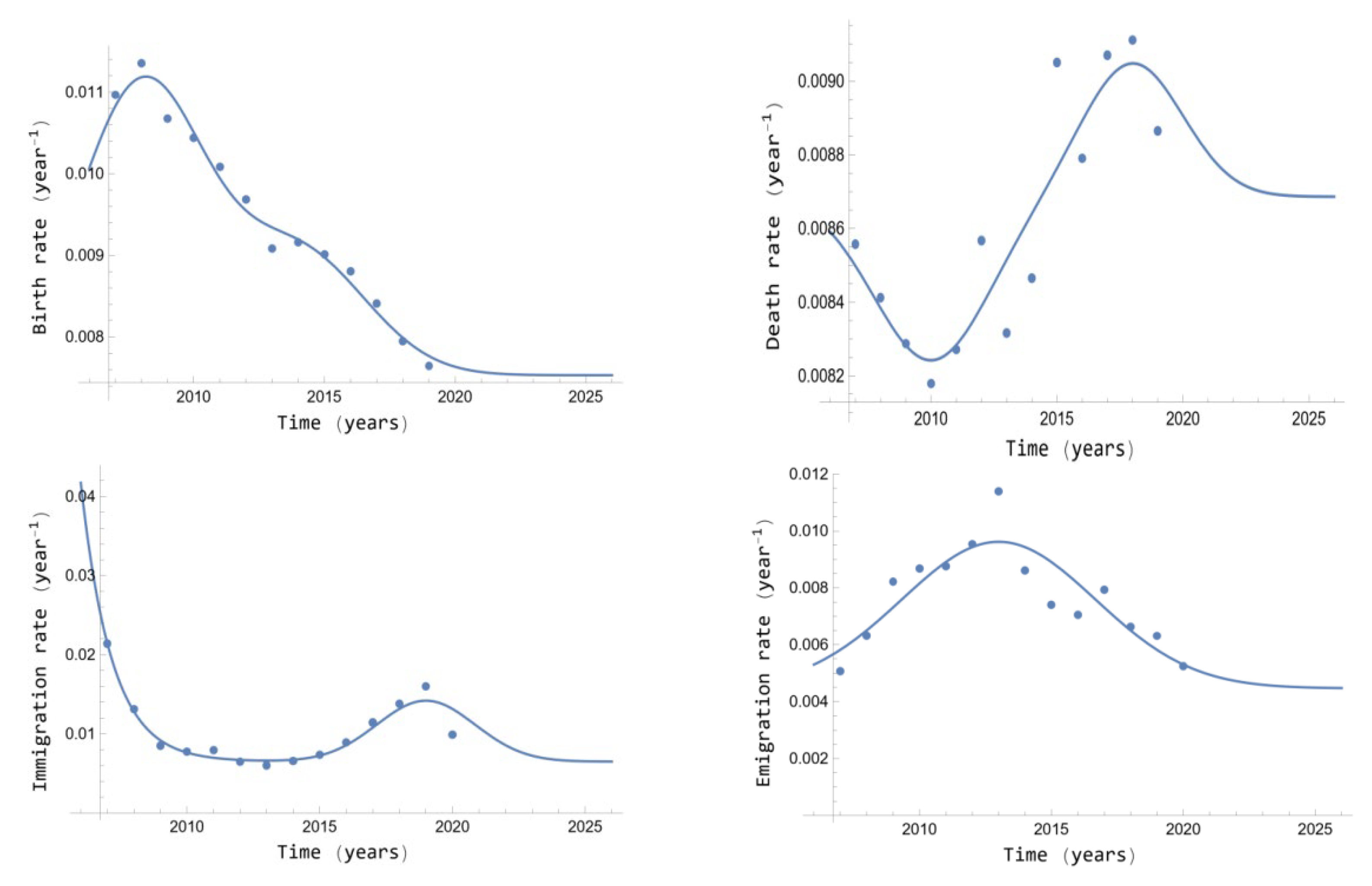
About the change rates, the data corresponding to the total population in the period 2007–2021 are known, but the known data of the total births and deaths at the moment of writing this paper correspond to the 2007–2019 period. The dynamical patterns for the crude birth and death rates were obtained by fitting the data of the 2007–2019 period. The known data of the total immigrations and emigrations at the moment of writing this paper correspond to the period 2007–2020, then the dynamical patterns for the crude immigration and emigration rates were obtained by fitting the data of the 2007–2020 period.

On the other hand, the dynamical patterns fitted to the historical data corresponding to these periods must be bounded for $t\ge t_0$ ($t_0=2007$), because, to be realistic, their future forecasting must not diverge. This is the reason that, for instance, an interpolating polynomial cannot be used to reproduce these dynamical patterns. The bounded functions used are either logistic functions or Gaussian functions, such as was already used in the works [3,4,5,6,7,8,9] successfully. To show graphically this boundedness, the fitting functions are represented in a longer period: 2007–2026, adding the five years period of future forecasting. In addition, these dynamical patterns were obtained with random residuals by using the NonlinearModelFit function of MATHEMATICA 12.3. The fitting results are provided in the beginning. For the birth rate,

$$a\left(t\right)=0.0075+0.0015·{\mathrm{e}}^{-0.07{\left(-2014+t\right)}^2}+0.0035·{\mathrm{e}}^{-0.08{\left(-2028+t\right)}^2}$$

(38)

For the death rate,

$$b\left(t\right)=0.0087+0.0004·{\mathrm{e}}^{-0.125{\left(-2018+t\right)}^2}+0.0004·{\mathrm{e}}^{-0.096{\left(-2010+t\right)}^2}$$

(39)

For the immigration rate,

$$f\left(t\right)=-909.476+0.008·{\mathrm{e}}^{-0.15{\left(-2019+t\right)}^2}+\frac{909.483}{1-0.00002·{\mathrm{e}}^{0.86\left(2007-t\right)}}$$

(40)

For the emigration rate,

$$g\left(t\right)=0.004+0.005·{\mathrm{e}}^{-0.037{\left(-2013+t\right)}^2}$$

(41)

Figure 1 shows the fitting functions versus time jointly the corresponding real data. The determination coefficients are $R^2=0.980$ for the birth rate, $R^2=0.823$ for the death rate, $R^2=0.933$ for the immigration rate, and $R^2=0.750$ for the emigration rate. Note that the different determination coefficients vary from 0.750 to 0.980. However, they can be considered acceptable due to the random variability between the real and model data observed in the figure. Actually, in order to use the model provided by Equation (36) to forecast the future, the dynamical patterns of the input variables given by Equations (38)–(41) must be found from the historical data. The limits of the future forecasts are analyzed in Section 4.2.

As explained above, the initial population densities are those corresponding to the 2007 and the 2021 years for Equation (9) of the PPDM, which is part of its analytical solution Equation (36). Note that the initial population densities must hold Equation (11); then, their corresponding mathematical patterns are obtained with the NonlinearModelFit function of MATHEMATICA 12.3 by linear combinations of Gaussian functions centered in the main peaks provided by the real data. These functions ensure their convergence to zero in the infinite age.

Concretely for the 2007 year,

$$\begin{gathered} u\left(x\right)=327168.35·{\mathrm{e}}^{-0.007{\left(-75.52+x\right)}^2}+77664.38·{\mathrm{e}}^{-0.088{\left(-72.11+x\right)}^2} \\ +312163.63·{\mathrm{e}}^{-0.021{\left(-60.86+x\right)}^2}+568298.36·{\mathrm{e}}^{-0.010{\left(-47.49+x\right)}^2} \\ +76159.03·{\mathrm{e}}^{-0.059{\left(-40.42+x\right)}^2}+667237.40·{\mathrm{e}}^{-0.01{\left(-30.74+x\right)}^2} \\ +77828.97·{\mathrm{e}}^{-0.034{\left(-16.26+x\right)}^2}+510545.25·{\mathrm{e}}^{-0.001{\left(-6.14+x\right)}^2} \end{gathered}$$

(42)

And for the 2021 year:

$$\begin{gathered} u\left(x\right)=52079.28·{\mathrm{e}}^{-0.005{\left(-77.82+x\right)}^2}+707530.41·{\mathrm{e}}^{-0.003{\left(-52.23+x\right)}^2} \\ +176604.27·{\mathrm{e}}^{-0.028{\left(-42.66+x\right)}^2}+117776.35·{\mathrm{e}}^{-0.020{\left(-31.30+x\right)}^2} \\ +495024.34·{\mathrm{e}}^{-0.002{\left(-12.73+x\right)}^2} \end{gathered}$$

(43)

Figure 2 shows the population densities given by Equations (42) and (43) versus age (x). Note that graphically, the functions hardly present variability with respect to the real data. In fact, the determination coefficients are $R^2=0.997$ for the 2007 year and $R^2=0.995$ for the 2021 year.

4.2. Validation of the PPDM Analytical Solution

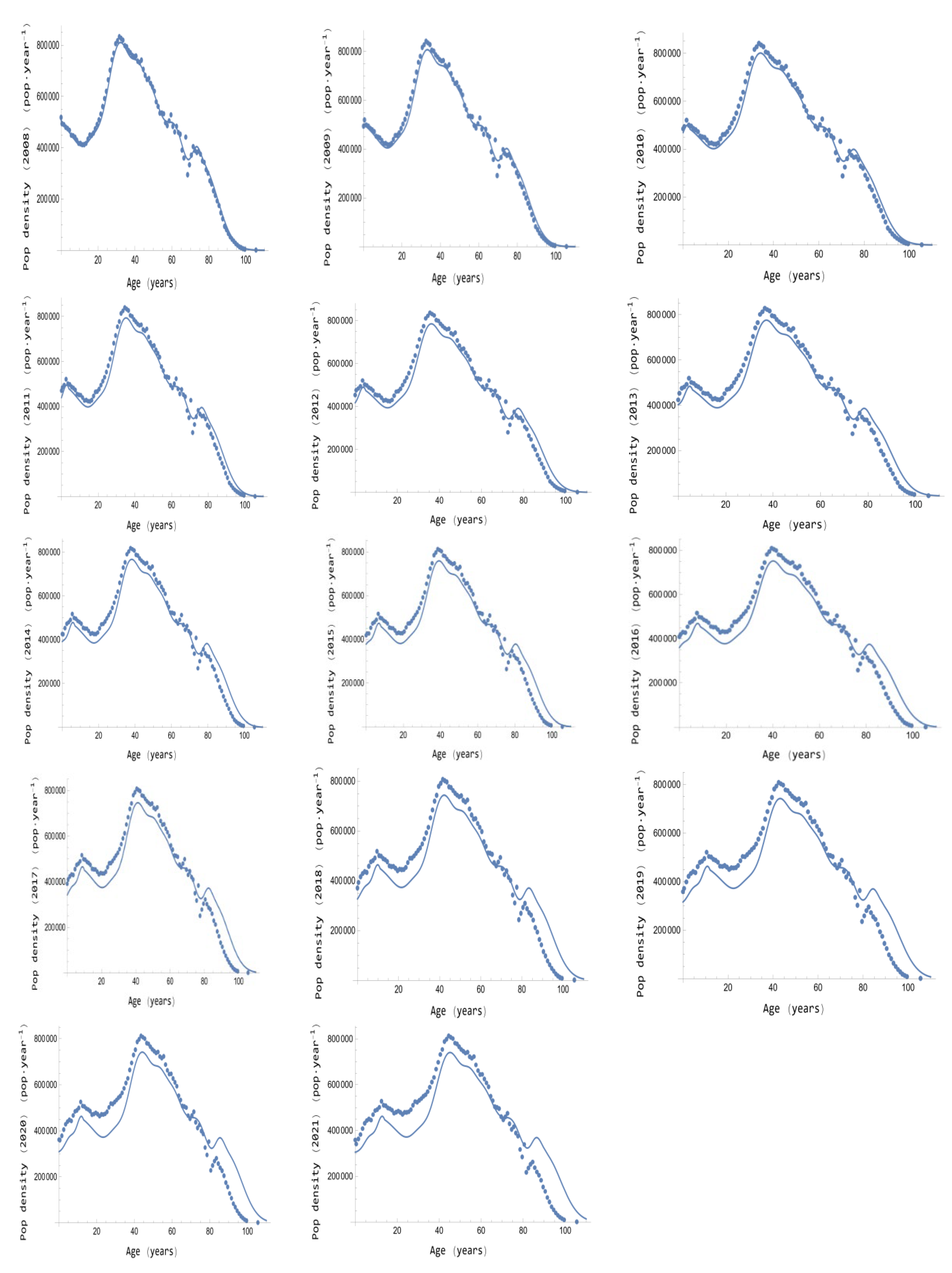
In this section, the historical data of the population densities are compared with those provided by the PPDM analytical solution of Equation (36) for the 2008–2021 period. Equation (36) takes into account the dynamical patterns for the change rates provided by Equations (38)–(41), and the initial population density provided by Equation (42).

Figure 3 shows the evolution of the population pyramid, i.e., the population densities for every year of this period, by representing the historical data jointly with the outcomes provided by the PPDM analytical solution Equation (36). The corresponding determination coefficients are presented in

Table 1. Determination coefficients ($R^2$ ) corresponding to Figure 3: the historical data of population densities compared with the outcomes obtained with the PPDM analytical solution in Spain in the 2008–201 period.

Year	2008	2009	2010	2011	2012	2013	2014
${\mathit{R}}^{\mathbf{2}}$	0.996	0.994	0.991	0.990	0.984	0.980	0.974
Year	2015	2016	2017	2018	2019	2020	2021
${\mathit{R}}^{\mathbf{2}}$	0.970	0.960	0.945	0.930	0.910	0.883	0.860

. In general, the figure shows close shapes between the historical pyramid populations and the model forecasting in this period. However, the model shape diverges as the time advances, in such a way that for low ages, the model tends to be under the historical data and for high ages, the model tends to be over the historical data. In addition, Table 1 presents the corresponding determination coefficients for every year. They decrease from $R^2=0.996$ in the 2008 year to $R^2=0.860$ in the 2021 year. Considering both the graphics of Figure 3 and the determination coefficients of Table 1, it can be asserted that the PPDM analytical solution has a high forecasting power.

However, the question that arises is how much is acceptable for this forecasting power, in other words, which are the limits of the PPDM analytical solution forecasting? For instance, considering a determination coefficient over 0.980 could be a good criterion: watching Table 1, the limit for an acceptable PPDM analytical solution forecasting would be 5 years. However, from a demographic point of view, more information is needed, and it can be provided by two fundamental variables in demography that can be derived from the PPDM analytical solution: the dependency ratio and life expectancy at birth.

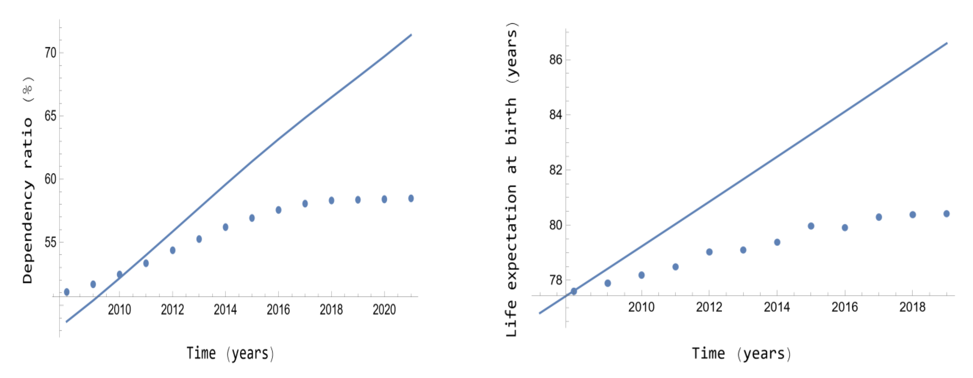
The dependency ratio is defined, in percentage, as the population in working age with respect to the population of non-working age. The historical values for a determined year can be computed from the population by ages by adding for three differenced populations the corresponding data and making the division multiplied by 100. If the PPDM analytical solution is used, and $x_m$ and $x_M$ are the corresponding minimum age to work and retirement age, the dependency ratio $dr\left(t\right)$ can be computed as

$$dr\left(t\right)=100\frac{{{\displaystyle \int }}_{x_m}^{x_M}w\left(t,x\right) dx}{{{\displaystyle \int }}_0^{x_m}w\left(t,x\right) dx+{{\displaystyle \int }}_{x_M}^{+\infty }w\left(t,x\right) dx}$$

(44)

In Equation (44), $w\left(t,x\right)$ is that provided by Equation (36). Figure 4 (left) shows the evolution of the dependency ratio historical data in Spain in the period of validation 2008–2021. Note that in the first years, the historical data and the outcomes provided by Equation (44) are very close, but they diverge as the time increases from the initial condition, such as it also happens with the population pyramid evolution of Figure 3 and the determination coefficients of Table 1. However, in order to precisely determine the differences between both sets of data,

Table 2. Relative errors in percentage (RE) for the dependency ratio in Spain in the 2008–2021 period.

Year	2008	2009	2010	2011	2012	2013	2014
RE (%)	4.60	2.48	0.56	1.23	2.73	4.45	5.99
Year	2015	2016	2017	2018	2019	2020	2021
RE (%)	7.85	9.74	11.67	13.98	16.63	19.36	22.11

provides the relative errors, computed as the percentage of the absolute difference between both data divided by the historical data. Table 2 confirms the first assumption of five years that the limits of the PPDM analytical solution forecasting due to the relative errors for the dependency ratio vary between 0.56% and 4.60% in the first five years.

Life expectancy at birth is defined as the average years of death in a determined population for every year. In order to compute its historical data from deaths by ages, the continuous addition (integral) of the age multiplied by the probability to die in this age must be computed. This probability is computed by the division of the deaths in each age divided by the total deaths for every year. In order to obtain its evolution for Spain in the 2008–2019 period, the age-structured deaths were obtained from Eurostat. Note that at the time, to set up this paper, the deaths of the 2020 and 2021 years were not present in Eurostat yet. To compute the life expectancy at birth evolution $leb\left(t\right)$ from the PPDM analytical solution, first the probability evolution to die in a determined age x, $prd\left(t,x\right)$, has to be computed:

$$prd\left(t,x\right)=\frac{def\left(t,x\right)}{{{\displaystyle \int }}_0^{+\infty }def\left(t,x\right) dx}=\frac{b\left(t\right)·w\left(t,x\right)}{b\left(t\right){{\displaystyle \int }}_0^{+\infty }w\left(t,x\right) dx}=\frac{w\left(t,x\right)}{{{\displaystyle \int }}_0^{+\infty }w\left(t,x\right) dx}$$

(45)

From Equation (45), $leb\left(t\right)$ can be computed:

$$leb\left(t\right)={\left({{\displaystyle \int }}_0^{+\infty }{x}^n·prd\left(t,x\right) dx\right)}^{1/n}={\left(\frac{1}{{{\displaystyle \int }}_0^{+\infty }w\left(t,x\right) dx}{{\displaystyle \int }}_0^{+\infty }{x}^n·w\left(t,x\right) dx\right)}^{1/n}$$

(46)

The definition of Equation (46) for life expectancy at birth is more general than the expectable definition for n = 1, which does not really work and does work with another n value (see below). In fact, the computation for n = 1 provides outcomes that differ at 50% from the historical data. However, after some computations to minimize the difference between the outcome provided by Equation (46) and the historical outcome in the 2008 year, the best value obtained is n = 21.9. Then, the evolution of the life expectancy at birth in Spain in the 2007–2019 period can be computed with similar values to those provided by the historical data.

Figure 4 (right) shows the evolution of the life expectancy at birth historical data jointly with the outcomes computed by Equation (46) with n = 21.9 in Spain for the 2008–2019 period. Note again that in the first years, the historical data and the outcomes provided by Equation (46) are very close, but they diverge as the time increases from the initial condition, such as it also happens with the population pyramid evolution of Figure 3, with the corresponding determination coefficients of Table 1, and with Figure 4 for the dependency ratio and the corresponding relative errors of Table 2. In order to support the precision provided,

Table 3. Relative errors in percentage (RE) for the life expectancy at birth in Spain in the 2008–2019 period.

Year	2008	2009	2010	2011	2012	2013	2014
RE (%)	1.02	0.35	0.30	0.94	1.27	2.21	2.88
Year	2015	2016	2017	2018	2019
RE (%)	3.15	4.24	4.77	5.68	6.66

provides the relative errors for the life expectancy at birth, computed in the same way as for the dependency ratio. Table 3 confirms the assumption of five years about the limits of the PPDM analytical solution forecasting due to the relative errors for the life expectancy at birth varying between 0.30% and 1.27% in the first five years.

4.3. Future Forecasting with the PPDM Analytical Solution

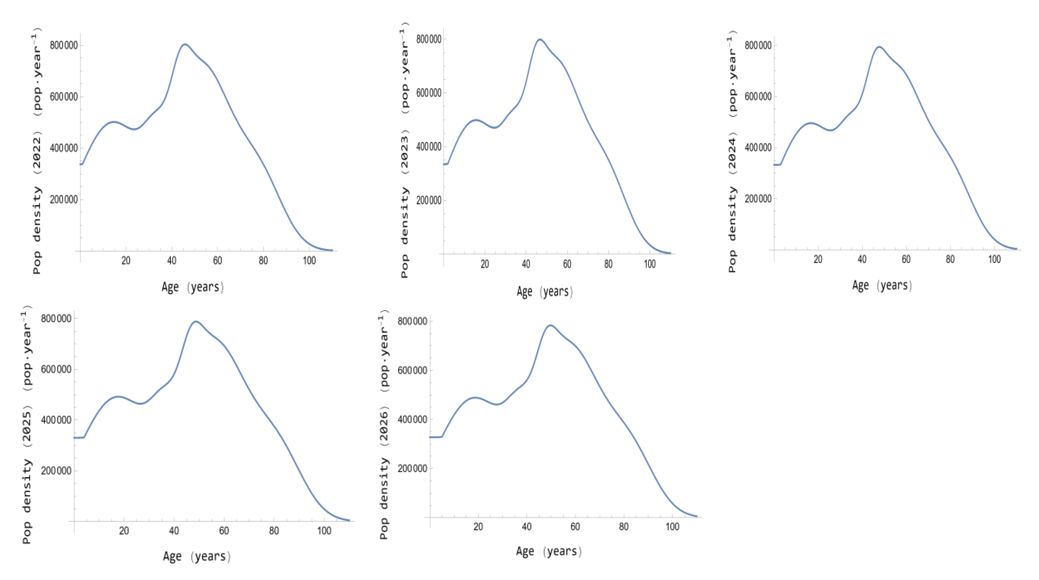
In the last section, a forecasting limit of five years is stated for the PPDM analytical solution. Therefore, in this section, the population pyramids, as well as the dependency ratio and the life expectancy at birth, are forecasted and commented in the 2022–2026 period for Spain, taking the initial population density in the 2021 year given by Equation (43). Note that the future evolutions of the change rates are given by Equations (38)–(41).

Figure 5 presents the forecasted evolution of the population pyramids in the 2022–2026 period. Observe that no appreciable change is expectable in its shape in this future period. The reason is the stable trends in the change rates in this period as Figure 1 shows. Although this stability cannot be expected in the future, it could be used as a base to assay new future scenarios or new future strategies to change the population pyramid shape, as was done in [29,30] with a numerical approach. Note that [29] is a first sketched approach of the complete investigation presented in [30].

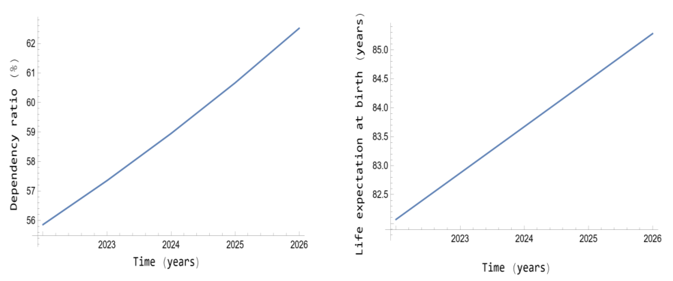
In addition, Figure 6 presents the forecasted evolution of the dependency ratio and the life expectancy at birth for the 2022–2026 period. Note that the dependency ratio can be considered very hopeless from a demographic point of view, and this is one of the reasons that the developed countries should change their strategies of births, immigration and emigration, as was tried in [29,30] with a numerical approach. This assertion is supported by the life expectancy at birth evolution: it increases so quickly that it can worsen the problem of the dependency ratio rising.

5. Other Models and Their Contrast with the PPDM

Further approaches that could generalize the PPDM are provided in the paper. For instance, if the change rates are inserted in an age-structured population model by considering only the age dependence, then the birth rate arises in the databases by mother’s age, i.e., as a fertility rate. Thus, to be realistic, the model has to be considered with different sex fertility rates and, by mathematical coherence, the population pyramid must be differenced by sexes. In other words, the simplification hypothesis that the change rates just depend on age in Equations (5)–(7) should be rewritten by sexes: $A_i\left(t,x\right)\approx a_i\left(x\right)$, $B_i\left(t,x\right)\approx b_i\left(x\right)$, $F_i\left(t,x\right)\approx f_i\left(x\right)$, $G_i\left(t,x\right)\approx g_i\left(x\right)$, where i = 1 represents males and i = 2 represents females, and also population densities must be differenced by sexes. With these considerations in the model given by Equations (5)–(7), it becomes

$$\frac{\partial w_i\left(t,x\right)}{\partial t}+c\frac{\partial w_i\left(t,x\right)}{\partial x}=\left(b_i\left(x\right)-f_i\left(x\right)+g_i\left(x\right)\right)w_i\left(t,x\right)$$

(47)

$$w_i\left(t_0,x\right)=u_i\left(x\right)\hspace{1em}x\ge 0$$

(48)

$$w_i\left(t,0\right)=\frac{1}{c}{{\displaystyle \int }}_0^{+\infty }{a}_i\left(x\right)·w_2\left(t,x\right) dx\hspace{1em}t\ge t_0$$

(49)

The author’s attempts to solve analytically the system of Equations (47)–(49) was fruitless, the central problem being obtaining the solution of the singular integral equation derived from Equation (49). However, this approach also presents a practical problem: the dynamical patterns of the change rates are not present in Equations (47)–(49) as temporal functions; then, neither links of these dynamics can be performed with other social variables, nor can policies about these dynamics be assayed on Equations (47)–(49).

Therefore, another more realistic approximation can be performed: $A_i\left(t,x\right)\approx {\alpha }_i\left(x\right)·a_i\left(t\right)$, $B_i\left(t,x\right)\approx {\beta }_i\left(x\right)·b_i\left(t\right)$, $F_i\left(t,x\right)\approx {\delta }_i\left(x\right)·f_i\left(t\right)$, $G_i\left(t,x\right)\approx {\gamma }_i\left(x\right)·g_i\left(t\right)$, where i = 1 represents males and i = 2 represents females, where ${\alpha }_i\left(x\right)$, ${\beta }_i\left(x\right)$, ${\delta }_i\left(x\right)$ and ${\gamma }_i\left(x\right)$ are the age-structured change rates divided by their total amounts in the initial time ($t=t_0$) by sexes, i.e., their initial age-structured weights in the initial time ($t=t_0$) by sexes. Considering these new hypotheses, Equations (5)–(7) are rewritten as

$$\frac{\partial w_i\left(t,x\right)}{\partial t}+c\frac{\partial w_i\left(t,x\right)}{\partial x}=\left({\beta }_i\left(x\right)·b_i\left(t\right)-{\delta }_i\left(x\right)·f_i\left(t\right)+{\gamma }_i\left(x\right)·g_i\left(t\right)\right)w_i\left(t,x\right)$$

(50)

$$w_i\left(t_0,x\right)=u_i\left(x\right)\hspace{1em}\hspace{1em}\hspace{1em}x\ge 0$$

(51)

$$w_i\left(t,0\right)=\frac{a_i\left(t\right)}{c}{{\displaystyle \int }}_0^{+\infty }{\alpha }_i\left(x\right)·w_2\left(t,x\right) dx\hspace{1em}\hspace{1em}\hspace{1em}t\ge t_0$$

(52)

Again, the author’s attempts to solve analytically the system of Equations (50)–(52) were fruitless by the moment, being again the central problem getting the solution of the singular integral equation derived from Equation (52).

The approaches given by Equations (47)–(49) or by Equations (50)–(51) are interesting if, for instance, the dynamics of life expectancy at birth is going to be evaluated by sexes. Subsequent analytical or numerical studies should compare their respective results in order to assess which of the models provides better forecasting. In addition, both sets of equations are also suitable if the focus of study is the total population pyramid $w\left(t,x\right)$ (without sex difference), due to $w\left(t,x\right)=w_1\left(t,x\right)+w_2\left(t,x\right)$ (the age groups must be equally defined for both sexes).

However, if the focus of study is, for instance, the dependency ratio, and the contribution of the sex-structure for the change rates is proved fundamental, then policies that influence on the change rates by sexes cannot be planned, and the non-sex change rates should arise in the model given by Equations (50)–(52). This application is impossible by using Equations (47)–(49) but it is possible by using Equations (50)–(52). The way to insert the non-sex change rates is easy, by their respective sex weights, i.e., by doing the following changes in Equations (50)–(52):

$$a_i\left(t\right)=\frac{n{a}_i\left(t\right)}{n{a}_1\left(t\right)+n{a}_2\left(t\right)}a\left(t\right)$$

(53)

$$b_i\left(t\right)=\frac{n{b}_i\left(t\right)}{n{b}_1\left(t\right)+n{b}_2\left(t\right)}b\left(t\right)$$

(54)

$$f_i\left(t\right)=\frac{n{f}_i\left(t\right)}{n{f}_1\left(t\right)+n{f}_2\left(t\right)}f\left(t\right)$$

(55)

$$g_i\left(t\right)=\frac{n{g}_i\left(t\right)}{n{g}_1\left(t\right)+n{g}_2\left(t\right)}g\left(t\right)$$

(56)

For instance, in Equation (53), $n{a}_i\left(t\right)$ is the amount of male births dynamical pattern, for i = 1, and the amount of female births dynamical pattern, for i = 2. In the same sense, Equations (54)–(56) must be interpreted for the other change rates. Finding these dynamical patterns is possible because the databases usually provide these data by sexes; in fact, the Eurostat databases provide them. The work [30] is an attempt to use Equations (50)–(52) jointly with Equations (53)–(56) to approach numerically the problem of the dependency ratio minimization by using a genetic algorithm.

6. Conclusions

Note that the main objectives of this paper are reached: on the one hand, to provide the population pyramid dynamics model (PPDM), with which to study the evolution of the population pyramid, as well as other variables, such as the evolution of the dependency ratio or of the life expectancy at birth, in a determined country or society.

On the other hand, obtaining the PPDM exact analytical solution was reached. As commented in the Introduction section, finding the analytical solution emphasizes the epistemological status of human sciences [34]. However, another hard reason to obtain the PPDM exact analytical solution Equation (36) is that it allows other scientists to better study qualitative properties of the population pyramid. For instance, an explicit property that arises from the PPDM analytical solution is that only using the birth rate as control variable to change the population pyramid shape by minimizing the dependency ratio is not realistic, such as was already noted in the works [3,4]. The reason is that the birth rate arises only explicitly in Equation (36) for the domain $x\le c\left(t-t_0\right)$, then the planned policies would need about 100 years to change this shape by influencing only the births. However, the other change rates do arise explicitly for the domain $x\ge c\left(t-t_0\right)$. Therefore, additional suitable policies about immigration and emigration must also be considered to change the population pyramid shape at short term. The works [29,30] are attempts to solve these problems by numerical methods.

However, the studies that use numerical methods must be considered complementary approaches of the analytical approaches, and it must be emphasized that both approaches must be developed concurrently. The reason is that if other hypotheses present an age-structured population model such the only age dependency of the change rates in [28], an analytical solution becomes impossible by the moment, because the corresponding boundary condition becomes a singular integral equation that is impossible to be exactly solved, unless some approximations can be done, such as in [3,4].

In addition, the forecasting power of the PPDM analytical solution could be improved by generalizing the model including the age dependence in the change rates. However, as seen in Section 5, the dynamical patterns as temporal functions of the time changes must be conserved. The reasons are crucial: (a) they allow planning policies about the population pyramid shape, for instance, through the dependency ratio minimization: (b) through relating the change rates with other social variables, such as well-being or happiness, increasing like this the model complexity to solve other problems of a socioeconomic nature [5,6,7,8,9]. Note that part (b) implies that the change rates are not already input variables depending on time; they become output variables that can depend on the other social variables, for instance, well-being.

As seen in Section 5, the alternative model that could better improve the forecasting power of the PPDM analytical solution would be that corresponding to Equations (50)–(52), including the changes given by Equations (53)–(56), if necessary. This author’s paper point of view is that this generalized model would also improve the forecasting power of the dependency ratio and the expectancy life at birth, in addition to the corresponding population pyramid evolution. The numerical results of the work [30] support this hypothesis. Perhaps the analytical solution of the generalized model could provide that the theoretical definition of the life expectancy at birth given by Equation (46) could be defined for n = 1, in better coherence with the definition of this variable from its historical data. However, the objective in a close future of this paper author’s is to try to obtain the analytical solution of the generalized model given by Equations (50)–(52), including, if necessary, the changes given by Equations (53)–(56).

Therefore, as conclusion, the unsettled main problem is to go beyond the approximation provided by the analytical solution given by Equation (36), where no difference between the female and male population density is presented, obtaining the analytical solution of Equations (50)–(52) (including, if needed, the changes of Equations (53)–(56)). In fact, since the numerical solution of Equations (50)–(56) was successfully obtained in [30], this approach, illustrated in Section 4, is expected to lead to a satisfactory analytical solution.

References

- Inaba, H. Age-Structured Population Dynamics in Demography and Epidemiology; Springer: Singapore, 2017. [Google Scholar]
- Innelli, M.; Milner, F. The Basic Approach to Age-Structured Population Dynamics; Springer: Dordrecht, The Netherlands, 2017. [Google Scholar]
- Micó, J.C.; Soler, D.; Caselles, A. Age-Structured Human Population Dynamics. J. Math. Sociol. 2006, 30, 1–31. [Google Scholar] [CrossRef]
- Micó, J.C.; Soler, D.; Caselles, A. A Side-by-Side Single Sex Age-Structured Human Population Dynamic Model: Exact Solution and Model Validation. J. Math. Sociol. 2008, 32, 285–321. [Google Scholar] [CrossRef]
- Sanz, M.T.; Micó, J.C.; Caselles, A.; Soler, D. A Stochastic Model for Population and Well-Being Dynamics. J. Math. Sociol. 2014, 38, 75–94. [Google Scholar] [CrossRef]
- Caselles, A.; Soler, D.; Sanz, M.T.; Micó, J.C. Simulating Demography and Human Development Dynamics. Cybern. Syst. An. Int. J. 2014, 45, 465–485. [Google Scholar] [CrossRef]
- Sanz, M.T.; Caselles, A.; Micó, J.; Soler, D. Including an environmental quality index in a demographic model. Int. J. Glob. Warm. 2019, 9, 362–396. [Google Scholar] [CrossRef]
- Soler, D.; Sanz, M.T.; Caselles, A.; Micó, J.C. A stochastic dynamic model to evaluate the influence of economy and well-being on unemployment control. J. Comput. Appl. Math. 2018, 330, 1063–1080. [Google Scholar] [CrossRef]
- Sanz, M.T.; Caselles, A.; Micó, J.; Soler, D. A stochastic dynamical social model involving a human happiness index. J. Comput. Appl. Math. 2016, 35, 867−890. [Google Scholar] [CrossRef]
- Wilson, T. Visualising the demographic factors which shape population age structure. Demogr. Res. 2008, 42, 1173–1185. [Google Scholar] [CrossRef]
- Edmonston, B. Canadian Provincial Population Growth: Fertility, Migration, and Age Structure Effects. Can. Stud. Popul. 2009, 36, 111–144. [Google Scholar] [CrossRef]
- González-Parra, G.; Jódar, L.; Santonja, F.J.; Villanueva, R.J. An Age-Structured Model for Childhood Obesity. Math. Popul. Stud. 2010, 17, 1–11. [Google Scholar] [CrossRef]
- Webb, G.F. Theory of Nonlinear Age-Dependent Population Dynamics; Marcel Dekker: New York, NY, USA, 1985. [Google Scholar]
- Li, X. Variational iteration method for nonlinear age-structured population models. Comput. Math. Appl. 2009, 58, 2177–2181. [Google Scholar] [CrossRef]
- Vogelsang, E.M.; Raymo, J.M. Local-Area Age Structure and Population Composition: Implications for Elderly Health in Japan. J. Aging Health 2014, 26, 155–177. [Google Scholar] [CrossRef]
- Zang, H.A.; Zhang, H.O.; Zhang, J. Demographic age structure and economic development: Evidence from Chinese provinces. J. Comp. Econ. 2015, 43, 170–185. [Google Scholar] [CrossRef]
- Vogel, M.; Porter, L.C. Toward a Demographic Understanding of Incarceration Disparities: Race, Ethnicity, and Age Structure. J. Quant. Criminol. 2016, 32, 515–530. [Google Scholar] [CrossRef]
- Castelló-Climent, A. The Age Structure of Human Capital and Economic Growth. Oxf. Bull. Econ. Stat. 2019, 81, 394–411. [Google Scholar] [CrossRef]
- Kotschy, R.; Urtaza, P.S.; Sunde, U. The demographic dividend is more than an education dividend. Proc. Natl. Acad. Sci. USA 2020, 117, 25982–25984. [Google Scholar] [CrossRef]
- Kumar, D.; Bisht, N.; Kumar, I. The role of age structure and occupational choices in the Indian labour market. Int. J. Soc. Econ. 2021, 48, 1718–1739. [Google Scholar] [CrossRef]
- Paquin-Lefebvre, P.; Bélair, J. On the Effect of Age-Dependent Mortality on the Stability of a System of Delay-Differential Equations Modeling Erythropoiesis. Acta Biotheor. 2021, 68, 5–19. [Google Scholar] [CrossRef]
- Khan, A.; Zaman, G.; Ullah, R., III; Naveed, N. Optimal control strategies for a heroin epidemic model with age-dependent susceptibility and recovery-age. AIMS Math. 2020, 6, 1377–1394. [Google Scholar] [CrossRef]
- Griette, Q.; Magal, P.; Seydi, O. Unreported Cases for Age Dependent COVID-19 Outbreak in Japan. Biology 2020, 9, 132. [Google Scholar] [CrossRef]
- Hostetter, N.H.; Lunn, N.J.; Richardson, V.S.; Regehr, E.V.; Converse, S.J. Age-structured Jolly-Seber model expands inference and improves parameter estimation from capture-recapture data. PLoS ONE 2021, 16, e0252748. [Google Scholar] [CrossRef]
- Zhang, S.; Liu, Y.; Cao, H. Bifurcation analysis of an age-structured epidemic model with two staged-progressions. Math. Methods Appl. Sci. 2021, 44, 11482–11497. [Google Scholar] [CrossRef]
- Yanyan, D.; Qimin, Z.; Meyer-Baese, A. The positive numerical solution for stochastic age-dependent capital system based on explicit-implicit algorithm. Appl. Numer. Math. 2021, 165, 198–215. [Google Scholar]
- Hathout, F.Z.; Touaoula, T.M. Mathematical analysis of a triple age dependent epidiemological model with including a protection strategy. Discret. Contin. Dyn. Syst. Ser. B 2022, 27, 7409–7443. [Google Scholar] [CrossRef]
- Abia, L.M.; Angulo, O.; López-Marcos, J.C.; López-Marcos, M.A. Numerical approximation of finite life-span age-structured population models. Math. Methods Appl. Sci. 2022, 45, 3272–3283. [Google Scholar] [CrossRef]
- Micó, J.C.; Soler, D.; Sanz, M.T.; Caselles, A.; Amigó, S. Birth Rate and Population Pyramid: A Stochastic Dynamical Model; Modelling for Engineering & Human Behaviour: Valéncia, Spain, 2018. [Google Scholar]
- Micó, J.C.; Soler, D.; Sanz, M.T.; Caselles, A.; Amigó, S. Minimizing Dependency Ratio in Spain through Demographic Variables. Mathematics 2022, 10, 1471. [Google Scholar] [CrossRef]
- Caselles, A.; Micó, J.C.; Amigó, S. Advances in the Physical Approach to Personality Dynamics; Modelling for Engineering & Human Behaviour: Valéncia, Spain, 2021. [Google Scholar]
- Amigó, S.; Caselles, A.; Micó, J.C.; Sanz, M.T.; Soler, D. Dynamics of the general factor of personality: A predictor mathematical tool of alcohol misuse. Math. Methods Appl. Sci. 2020, 43, 116–8135. [Google Scholar] [CrossRef]
- Caselles, A.; Micó, J.C.; Amigó, S. Energy and Personality: A Bridge between Physics and Psychology. Mathematics 2021, 9, 1339. [Google Scholar] [CrossRef]
- Ferrer, L.; Del Paradigma, M.; de la Ciencia, P.S. From the Mechanicist Paradigm of Science to System Paradigm; Universitat de València: Valencia, Spain, 1997. [Google Scholar]
- Esgolts, L. Differential Equations and the Calculus of Variations; Mir Publisher: Moscow, Russia, 1977. [Google Scholar]
Figure 1.
Change rates versus time in Spain: 2007–2026 period. Experimental values (dots) and theoretical values (line).
Figure 2.
Population densities versus age in Spain for 2007 and 2021 years. Experimental values (dots) and theoretical values (line).
Figure 3.
Population densities versus age in Spain for the 2008–2021 period. Experimental values (dots) and theoretical values (line). See the determination coefficients in Table 1.
Figure 4.
Dependency ratio versus time for the 2008–2021 period (left), and life expectancy at birth versus time for the 2008–2019 period (right), in Spain. Experimental values (dots) and theoretical values (line).
Figure 5.
Population densities versus age forecasted in Spain for the 2022–2026 period.
Figure 6.
Dependency ratio (left) and life expectancy at birth (right) versus time forecasted in Spain for the 2022–2026 period.