Instability of Viscoelastic Liquid Sheets in a Transverse Electric Field

Abstract

The temporal linear instability of a viscoelastic liquid sheet moving around an inviscid gas in a transverse electrical field is analyzed. The fluid is described by the leaky dielectric model, which is more complex than existing models and enables a characterization of the liquid electrical properties. In addition, the liquid is assumed to be viscoelastic, and the dimensionless dispersion relation of the sinuous and varicose modes between the wavenumber and the temporal growth rate can be derived as a 3 × 3 matrix. According to this relationship, the effects of the liquid properties on the sheet instability are determined. The results suggest that, as the electrical Euler number and the elasticity number increase and the time constant ratio decreases, the sheet becomes more unstable. Finally, an energy budget approach is adopted to investigate the instability mechanism for the sinuous mode.

1. Introduction

Sheet instabilities have been extensively studied in recent years because of their vital importance in the fields of mathematical physics and industry [1,2]. In scientific fields, such instabilities are classic issues in solving differential equations that are especially worthy for studying the behavior of the liquid sheet in an electrical field. Moreover, the instabilities of a liquid sheet are regularly encountered in spray combustion processes, ultra-fine water mist fire suppression systems [3], gas turbines, inkjet printing, and even liquid rocket engines [4].

Squire [5] conducted pioneering work on sheet instabilities by exploring the instability of a thin inviscid sheet surrounded by still air. Hagerty and Shea [6] developed this theory through linear analysis and concluded that there existed two modes, namely, the sinuous mode and the varicose mode. On this foundation, numerous researchers became interested in sheet electrodynamic behavior, and the stability of the sheet in an electric field was extensively investigated. In earlier studies, the sheets were considered as perfect conductors or dielectrics. Melcher and Schwarz [7,8] described how the disturbed surface waves of the viscous liquid sheet, which was treated as a perfectly insulating fluid, propagated along the lines of electric field intensity. They showed that the dominant effect of the charge relaxation was to improve the instability. El-Sayed [9] extended the analysis of Melcher [8] to the case of a fluid moving in the same direction as an air stream. It was concluded that the aerodynamic force reduced the stability when the Weber number was less than some critical value, whereas the electric force increased the stability. Under the perfect conductor model, Yang et al. [10] conducted an electrified viscoelastic liquid sheet injected into a dielectric stationary ambient gas.

In 1969, Taylor and Melcher [11] published a breakthrough paper in which they proposed a more accurate electric–leaky dielectric model (the Taylor–Melcher model). Saville [12] comprehensively summarized the basic equations of this model and, through the analysis of numerous experimental results, concluded that the theory was consistent with the practice. Research in this field then flourished. Cimpeanu [13] theoretically examined the classical Rayleigh–Taylor instability of thin films in a horizontal electric field, and Savettaseranee [14] examined the competition among surface tension, van der Waals, viscous, and electrically induced forces when a sheet was placed in an electric field parallel to its velocity. Moreover, Tilly et al. [15] concentrated on the nonlinear stability of an inviscid sheet between two electrodes. They found that the electric field led to a nonlinear stability for the sheet, delaying the formation of its singularity.

In fact, for many industrial and commercial applications, such as atomization and liquid rocket engines, the fluid of the sheet is non-Newtonian and can be characterized by viscoelastic properties. Therefore, it is necessary to understand the instability and breakup of viscoelastic sheets. Liu [16] performed a linearized stability analysis in which two-dimensional non-Newtonian liquid sheets moved in an inviscid gaseous environment. It was found that non-Newtonian liquid sheets had a higher growth rate than Newtonian liquid sheets for both symmetric and antisymmetric disturbances. Brenn et al. [17] extended this analysis to three-dimensional disturbances. Jia et al. [18] manipulated the linear temporal instability of viscoelastic planar liquid sheets in the presence of gas velocity oscillations. They found that the absence of shear viscosity, the stress relaxation time, and the deformation retardation time all affected the unstable regions.

To date, there have been few studies considering the instability of a viscoelastic sheet in an electric field, especially those that simulated the liquid sheet using the leaky dielectric model. The present study focused on the linear temporal instability of viscoelastic liquid sheets subjected to a transverse electric field and explained the physical mechanism using an energy approach. The influence of various parameters related to the non-Newtonian characteristics (the elasticity number and the time constant ratio) of the fluid on the stability of the jet is considered in detail. This research can better understand the mechanism of liquid film breaking. It has important academic value for science and engineering applications. In practical engineering applications, such as liquid rocket engines, most propellants are non-Newtonian fluids. Our contributions were important for two reasons. Firstly, we considered the effect of electrical properties that were similar to real-world scenarios alongside the viscoelasticity of the liquid sheet, which has not previously been explored. Secondly, this study used energy analysis to quantitatively describe the contribution of various forces, including the electric force and the elastic force, to the sheet stability.

The remainder of this paper is organized as follows. Section 2 describes the theoretical model and derives the dispersion relation by solving the governing equations and boundary conditions. Section 3 presents an energy analysis to explain the mechanism of the instability. Section 4 analyzes the influence of physical parameters. Finally, the conclusions to this study are presented in Section 5.

2. Theoretical Model

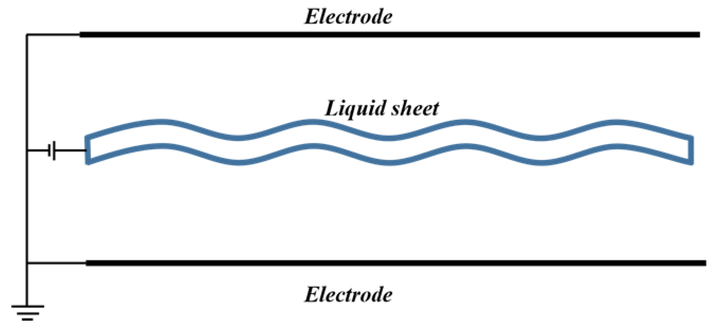
In the case of this paper, the physical model is extracted from the atomization experiment. The liquid film is sprayed into the static air (U_g = 0) from the nozzle, and the electric field is applied to the external field to study the physical mechanism at the initial stage of the atomization process. As shown in Figure 1, a viscoelastic sheet moving through an inviscid gas in a transverse electric field is considered. The coordinates are chosen such that the x-axis is parallel to the direction of the liquid sheet flow and the y-axis is normal to the liquid sheet. The leaky dielectric model is employed to describe the electrical properties of the liquid with finite conductivity and permittivity, while the gas is assumed to be a perfect dielectric with the associated permittivity in a vacuum. The liquid sheet is characterized by a viscoelastic model that includes three main parameters: zero shear viscosity ${\mu }_0$, the stress relaxation time ${\lambda }_1$, and the deformation retardation time ${\lambda }_2$. Gravity is ignored because the liquid film is very thin, and gravity is negligible compared to other forces for this model.

In the present case, the relationship between the stress tensor and the velocity field can be described by the Oldroyd-B constant equation [19,20], which can be written as

$$\begin{array}{l}\mathsf{\tau }+{\lambda }_1\left(\frac{\partial \mathsf{\tau }}{\partial t}+\left(v\cdot \nabla \right)\mathsf{\tau }-\left(\nabla v\right)\cdot \mathsf{\tau }-\mathsf{\tau }\cdot {\left(\nabla v\right)}^T\right)\\ ={\mu }_0\left(\dot{\gamma }+{\lambda }_2\left[\frac{\partial \dot{\gamma }}{\partial t}+\left(v\cdot \nabla \right)\dot{\gamma }-\left(\nabla v\right)\cdot \dot{\gamma }-\dot{\gamma }\cdot {\left(\nabla v\right)}^T\right]\right),\end{array}$$

(1)

where $\mathsf{\tau }$ is the extra stress tensor and $\dot{\gamma }=\nabla v+{\left(\nabla v\right)}^{\mathrm{T}}$ is the strain rate tensor.

Physical quantities are defined with appropriate values, and the corresponding scales are presented in

Table 1. Scales of dimensionless parameters.

Dimensionless Parameter	Meaning	Scale
$x$	Distance parallel to the basic flow	$a$
$y$	Distance normal to the basic flow	$a$
$t$	Time	$a/U$
$u$	$x$-direction velocity	$U$
$v$	$y$-direction velocity	$V$
${\varphi }_g$	Gas phase velocity	$Ua$
$P_0$	Basic flow pressure	${\rho }_l{U}^2$
$P$	Liquid phase pressure	${\rho }_l{U}^2$
$\mathsf{\tau }$	Liquid stress tensor	${\rho }_l{U}^2$
${\eta }_0$	Initial disturbance amplitude	$a$
$d$	Distance from electrode to sheet surface	$a$
${\lambda }_1$	Stress relaxation time	$a/U$
${\lambda }_2$	Deformation retardation	$a/U$
${\eta }_0$	Initial disturbance amplitude	$a$

. Both the liquid and the gas are assumed to be incompressible and the force of gravity is ignored.

2.1. Governing Equations

The governing equations for the liquid and gas phases are given as follows. The mass conservation equations are

$$\nabla \cdot v=0,-a+\eta <y<a+\eta ,$$

(2)

$${\nabla }^2{\varphi }_g=0,y<-a+\eta \mathrm{or}y>a+\eta ,$$

(3)

where the liquid velocity vector is $v=\left(\begin{array}{ccc}u& v& 0\end{array}\right)$.

The equations of momentum for the liquid phase are expressed as

$$\frac{\partial v}{\partial t}+\left(v\cdot \nabla \right)v=-\nabla p+\nabla \cdot \tau ,-a+\eta <y<a+\eta ,$$

(4)

$$p_g=-\rho \left[\frac{\partial {\varphi }_g}{\partial t}+\frac{1}{2}{\left(\nabla {\varphi }_g\right)}^2\right],y>a+\eta or y<-a+\eta .$$

(5)

2.2. Solutions for Electrical Field

An electrical potential function $V$ is first introduced to satisfy the Laplace equations for the gas phase and the liquid phase, which are written as follows:

$${\nabla }^2{V}_g=0,$$

(6)

$${\nabla }^2{V}_l=0.$$

(7)

The strength of the electrical field can be expressed as

$$E=-\nabla V.$$

(8)

The electric boundary conditions for the gas are simple:

$$\begin{array}{l}{V}_g=V_0,y=a+\eta ,\\ V_g=0,y=a+d.\end{array}$$

(9)

The electric stress in the liquid phase $T_l{}^e$ and in the gas $T_g^e$ can be obtained as follows:

$$T_l{}^e=\epsilon E_l{E}_l-\frac{1}{2}\delta \epsilon E_l\cdot E_{l}I,T_g^e=E_g{E}_g-\frac{1}{2}\delta E_g\cdot E_{g}I,$$

(10)

where $\delta$ is the Kronecker delta and $I$ is the identity matrix.

The boundary conditions for the liquid sheet are much more complicated. The model requires the continuity of the tangential electrical field strength, Gauss’ law, and the conservation law of interface charge on the gas-to-liquid surface, which are expressed, respectively, as

$$n\times \left(E_l-E_g\right)=0 ,y=\pm a+\eta ,$$

(11)

$$\left({\epsilon }_1{E}_l-{\epsilon }_2{E}_g\right)\cdot n=q_s,y=\pm a+\eta ,$$

(12)

$$\frac{\partial q_s}{\partial t}+v\cdot \nabla q_s-q_{s}n\cdot \left(n\cdot \nabla \right)\cdot v-(\sigma E_l)\cdot n=q_s,y=\pm a+\eta .$$

(13)

2.3. Boundary Conditions

The kinematic boundary conditions for the liquid and gas phases are

$$\frac{\partial H}{\partial t}+v\cdot \nabla H=0,y=\pm a+\eta ,$$

(14)

$$\frac{\partial H}{\partial t}+\nabla {\varphi }_g\cdot \nabla H=0,y=\pm a+\eta ,$$

(15)

where $H=y-\eta \left(x,t\right)$ and $H=0$ denote the two gas-to-liquid interfaces.

Because the gas is inviscid and there exists a tangential electrical stress $T_t^e$, the dynamic boundary condition parallel to the interfaces should be

$$\left(n\cdot \mathsf{\tau }\right)\times n=T_t^e,y=\pm a+\eta ,$$

(16)

where $n=\nabla H/\left|\nabla H\right|$ is the interface unit normal vector.

The dynamic boundary condition normal to the interface is written as

$$-p+\left(n\cdot \mathsf{\tau }\right)\cdot n+\frac{1}{We}\left(\nabla \cdot n\right)-\rho \left[\frac{\partial {\varphi }_{gj}}{\partial t}+\frac{1}{2}{\left(\frac{\partial {\varphi }_{gj}}{\partial x}\right)}^2+\frac{1}{2}{\left(\frac{\partial {\varphi }_{gj}}{\partial y}\right)}^2\right]=T_t^e, y=\pm a+\eta .$$

(17)

2.4. Linear Stability Analysis

To solve Equations (1)–(17), we employ linear instability analysis [12,13] using the form of the normal mode. For a sufficiently small disturbance, the following equation is obtained:

$$\begin{array}{l}(\eta ,u,v,p,\mathsf{\tau },\dot{\gamma },{\varphi }_g,p_g,V_g,V_l)=\\ [\eta (y),u(y),v(y),p(y),\mathsf{\tau }\left(y\right),\dot{\gamma }\left(y\right),{\varphi }_g(y),p_g(y),V_g(y),V_l(y)]\cdot \exp (\mathrm{i}kx+\omega t),\end{array}$$

(18)

where $k$ is the wavenumber and $\omega$ is the complex frequency $\omega ={\omega }_r+i{\omega }_i$, where ${\omega }_r$ represents the temporal growth rate of the disturbance and ${\omega }_i$ represents the disturbance frequency). Substituting Equation (18) into Equation (1) yields

$$\mathsf{\tau }+{\lambda }_1\left(\frac{\partial \mathsf{\tau }}{\partial t}+\frac{\partial \mathsf{\tau }}{\partial x}\right)=\frac{1}{Re}\left[{\dot{\gamma }}_1+{\lambda }_2\left(\frac{\partial \dot{\gamma }}{\partial t}+\frac{\partial \dot{\gamma }}{\partial x}\right)\right],$$

(19)

$$R{e}_1=\frac{1+{\lambda }_1(\mathrm{i}k+\omega )}{1+{\lambda }_2(\mathrm{i}k+\omega )}Re,$$

(20)

where $R{e}_1$ is the effective Reynolds number for the viscoelastic fluid.

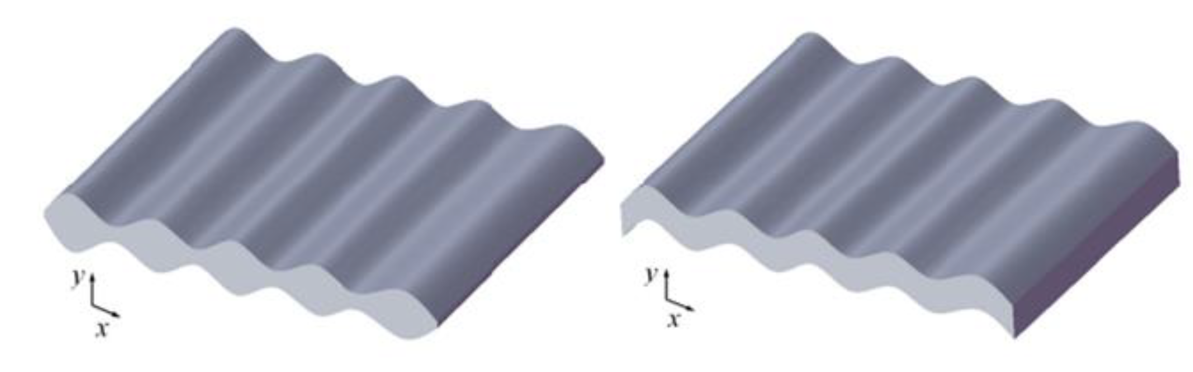
The two modes of liquid film are shown in Figure 2 below. The left figure describes the pattern in which the upper and lower boundaries are disturbed in the opposite direction, which is called varicose or symmetric, while the right figure is the pattern in which the upper and lower boundaries are disturbed in the same direction, which is called sinusoidal or antisymmetric.

Substituting Equation (18) into Equations (2)–(5) and the constitutive relation in Equation (19), the solution of the disturbance flow field can be obtained with a set of integration constants, which can be determined from the boundary conditions in Equations (14)–(17). The requirement of a nontrivial solution to the linear homogeneous equations leads to the dispersion relation.

$$D_{sin}\left({\omega }_1,k,R{e}_1\right)=0,\mathrm{or}{D}_{var}\left({\omega }_1,k,R{e}_1\right)=0,$$

(21)

where the subscripts ”sin” and ”var” represent the sinuous (antisymmetric) mode and the varicose (symmetric) mode, respectively. The two modes exist at the same time for the sheet instability, and their final expressions are as follows.

For the sinuous mode, the dispersion relation should be

$$\begin{array}{ll}\det (A)& =(\tau -\frac{L^2-K^2}{\mathrm{Re}}\frac{1+\lambda \cdot El(\mathrm{i}K+\Omega )}{1+El(\mathrm{i}K+\Omega )})(-2\cosh (K))D_{33}\\ & +\epsilon \frac{L^2-K^2}{\mathrm{Re}}\frac{1+\lambda \cdot El(\mathrm{i}K+\Omega )}{1+El(\mathrm{i}K+\Omega )}\frac{\cosh (K)}{KD\sinh (K)}\frac{V_0}{d}{D}_{32}\\ & +(\tau -\frac{L^2-K^2}{\mathrm{Re}}\frac{1+\lambda \cdot El(\mathrm{i}K+\Omega )}{1+El(\mathrm{i}K+\Omega )})\frac{V_0}{d}{D}_{32}\\ & -\epsilon \frac{L^2-K^2}{\mathrm{Re}}\frac{1+\lambda \cdot El(\mathrm{i}K+\Omega )}{1+El(\mathrm{i}K+\Omega )}2\cosh (K)D_{33}=0,\end{array}$$

(22)

where

$$\begin{array}{ll}\frac{V_0}{d}{D}_{32}& =-\frac{K^2+L^2}{K^2-L^2}2\coth (K)\cosh (K)\frac{KEu}{D^2}+\frac{4K^{2}L}{(K^2-L^2)}\frac{\cosh (K)}{\tanh (L)}\frac{Eu}{D^2}\\ & -2\sinh (K)\frac{KEu}{D^2},\\ D_{33}& =-\frac{{(K^2+L^2)}^2}{K}\frac{1}{{\mathrm{Re}}^2}\tanh (K)+\frac{4K^{2}L}{{\mathrm{Re}}^2}\tanh (L)-\frac{K^2}{We}-\overline{\rho }\frac{{\Omega }^2}{K}.\end{array}$$

(23)

Similarly, the varicose mode can be given as

$$\begin{array}{ll}\det (A)& =(\tau -\frac{L^2-K^2}{\mathrm{Re}}\frac{1+\lambda \cdot El(\mathrm{i}K+\Omega )}{1+El(\mathrm{i}K+\Omega )})(-2\sinh (K))D_{33}^{\prime }\\ & +\overline{\epsilon }\frac{L^2-K^2}{\mathrm{Re}}\frac{1+\lambda \cdot El(\mathrm{i}K+\Omega )}{1+El(\mathrm{i}K+\Omega )}\frac{\sinh (K)}{KD\cosh (K)}\frac{V_0}{d}{D}_{32}^{\prime }\\ & +(\tau -\frac{L^2-K^2}{\mathrm{Re}}\frac{1+\lambda \cdot El(\mathrm{i}K+\Omega )}{1+El(\mathrm{i}K+\Omega )})\frac{V_0}{d}{D}_{32}^{\prime }\\ & -\epsilon \frac{L^2-K^2}{\mathrm{Re}}\frac{1+\lambda \cdot El(\mathrm{i}K+\Omega )}{1+El(\mathrm{i}K+\Omega )}2\sinh (K)D_{33}^{\prime }=0.\end{array}$$

(24)

where

$$\begin{array}{ll}\frac{V_0}{d}{D}_{32}^{\prime }& =-\frac{K^2+L^2}{K^2-L^2}2\tanh (K)\sinh (K)\frac{KEu}{D^2}+\frac{4K^{2}L}{(K^2-L^2)}\frac{\sinh (K)}{\coth (L)}\frac{Eu}{D^2}\\ & -2\sinh (K)\frac{KEu}{D^2},\\ D_{33}^{\prime }& =-\frac{{(K^2+L^2)}^2}{K}\frac{1}{{\mathrm{Re}}^2}\coth (K)+\frac{4K^{2}L}{{\mathrm{Re}}^2}\coth (L)-\frac{K^2}{We}-\overline{\rho }\frac{{\Omega }^2}{K}\\ & -\frac{(K^2+L^2)}{K^2-L^2}\frac{KEu}{D^2}\tanh (K)+\frac{2K^{2}L}{(K^2-L^2)}\frac{Eu}{D^2}\tanh (L)+\frac{Eu}{D^3}.\end{array}$$

(25)

3. Energy Budget

To investigate the mechanism of the sheet instability, we conduct an energy budget analysis [21,22], which can trace the perturbation kinetic energy and the effects of various forces, especially the elastic force and the electric field force.

Firstly, we linearize the momentum equation and the constitutive relations of the liquid are as follows:

$$\frac{\partial v}{\partial t}+\frac{\partial v}{\partial x}=-\nabla p+\nabla \cdot \tau ,$$

(26)

$$\tau =\frac{1}{Re}\dot{\gamma }-{\lambda }_1^{}\left(\frac{\partial {\tau }_{}}{\partial t}+\frac{\partial {\tau }_{}}{\partial x}\right)+\frac{{\lambda }_2^{}}{Re}\left(\frac{\partial \dot{\gamma }}{\partial t}+\frac{\partial \dot{\gamma }}{\partial x}\right).$$

(27)

Combining Equations (24) and (25), the following equation is obtained

$$\frac{\partial v}{\partial t}+\frac{\partial v}{\partial x}=-\nabla p+\frac{1}{Re}{\nabla }^{2}v-{\lambda }_1^{}\nabla \cdot \left(\frac{\partial \tau }{\partial t}+\frac{\partial {\tau }_{}}{\partial x}\right)+\frac{{\lambda }_2^{}}{Re}\nabla \cdot \left(\frac{\partial {\dot{\gamma }}_{}}{\partial t}+\frac{\partial \dot{\gamma }}{\partial x}\right).$$

(28)

Secondly, we multiply both sides of Equation (26) by the perturbation velocity $v$ and integrate over one wavelength $\lambda =2\pi /k$ to get the energy equation. The results can be written as

$${\dot{e}}_k={\dot{w}}_p+{\dot{w}}_{vis}+{\dot{w}}_{El}+{\dot{w}}_{\overline{\lambda }},$$

(29)

where the left-hand side ${\dot{e}}_k$ represents the rate of change in the kinetic energy of the disturbance; the terms on the right-hand side represent different mechanisms: ${\dot{w}}_p$ is the total contribution of liquid pressure; ${\dot{w}}_{vis}$ is the viscous dissipation; ${\dot{w}}_{El}$ is the effect of elasticity; and ${\dot{w}}_{\overline{\lambda }}$ is the retardation of the deformation. The specific expressions for these terms are

$${\dot{e}}_k=\frac{k}{2\pi }{\displaystyle {\int }_0^{\frac{2\pi }{k}}{\displaystyle {\int }_{-1}^{1}v\cdot \left(\frac{\partial v}{\partial t}+\frac{\partial v}{\partial x}\right)}\mathrm{d}y\mathrm{d}x},$$

(30)

$${\dot{w}}_p=\frac{k}{2\pi }{\displaystyle {\int }_0^{\frac{2\pi }{k}}{\displaystyle {\int }_{-1}^1-v\cdot \nabla p}\mathrm{d}y\mathrm{d}x},$$

(31)

$${\dot{w}}_{vis}=\frac{k}{2\pi }{\displaystyle {\int }_0^{\frac{2\pi }{k}}{\displaystyle {\int }_{-1}^{1}v\cdot \frac{1}{Re}{\nabla }^{2}v}\mathrm{d}y\mathrm{d}x},$$

(32)

$${\dot{w}}_{El}=\frac{k}{2\pi }{\displaystyle {\int }_0^{\frac{2\pi }{k}}{\displaystyle {\int }_{-1}^1-v\cdot {\lambda }_1^{}\nabla \cdot \left(\frac{\partial \tau }{\partial t}+\frac{\partial \tau }{\partial x}\right)}\mathrm{d}y\mathrm{d}x},$$

(33)

$${\dot{w}}_{\overline{\lambda }}=\frac{k}{2\pi }{\displaystyle {\int }_0^{\frac{2\pi }{k}}{\displaystyle {\int }_{-1}^{1}v\cdot \frac{{\lambda }_2^{}}{Re}\nabla \cdot \left(\frac{\partial \dot{\gamma }}{\partial t}+\frac{\partial {\dot{\gamma }}_{}}{\partial x}\right)}\mathrm{d}y\mathrm{d}x}.$$

(34)

Finally, we substitute Equations (2) and (17) into Equation (29) and the results should be

$${\dot{w}}_p={\dot{w}}_g+{\dot{w}}_{\sigma }+{\dot{w}}_{\tau yy}+{\dot{w}}_{ew}+{\dot{w}}_{ez},$$

(35)

$${\dot{w}}_g=\frac{k}{2\pi }{\displaystyle {\int }_0^{\frac{2\pi }{k}}\rho \left[{\left(v\frac{\partial {\varphi }_g}{\partial t}\right)}_{y=a}-{\left(v\frac{\partial {\varphi }_g}{\partial t}\right)}_{y=-a}\right]}\mathrm{d}x,$$

(36)

$${\dot{w}}_{\sigma }=\frac{k}{2\pi }{\displaystyle {\int }_0^{\frac{2\pi }{k}}\frac{1}{We}\left[{\left(v\frac{{\partial }^2{\eta }_{}}{\partial x^2}\right)}_{y=a}+{\left(v\frac{{\partial }^2\eta }{\partial x^2}\right)}_{y=-a}\right]}\mathrm{d}x,$$

(37)

$${\dot{w}}_{\tau yy}=\frac{k}{2\pi }{\displaystyle {\int }_0^{\frac{2\pi }{k}}\left[-{\left(v{\tau }_{yy}\right)}_{y=a}+{\left(v{\tau }_{yy}\right)}_{y=-a}\right]}\mathrm{d}x,$$

(38)

$${\dot{w}}_{ew}=\frac{k}{2\pi }{\displaystyle {\int }_0^{\frac{2\pi }{k}}\left[-{\left(v_{}\frac{2E_u}{D^3}\right)}_{y=a}+{\left(v_{}\frac{2E_u}{D^3}\right)}_{y=-a}\right]}\mathrm{d}x,$$

(39)

$${\dot{w}}_{ez}=\frac{k}{2\pi }{\displaystyle {\int }_0^{\frac{2\pi }{k}}\left[-{\left(v_{}\frac{2K{E}_u}{D^2}sinh(k)\right)}_{y=a}+{\left(v_{}\frac{2K{E}_u}{D^2}sinh(k)\right)}_{y=-a}\right]}\mathrm{d}x,$$

(40)

where ${\dot{w}}_g$ is the result of gas pressure; ${\dot{w}}_{\sigma }$ is the effect of surface tension; ${\dot{w}}_{\tau yy}$ is the work of additional surface stress; ${\dot{w}}_{ew}$ is the product of the normal electrical force; and ${\dot{w}}_{ez}$ is the comprehensive effect of the tangential and normal electrical forces.

In summary, we have

$${\dot{e}}_k={\dot{w}}_{vis}+{\dot{w}}_{El}+{\dot{w}}_{\overline{\lambda }}+{\dot{w}}_g+{\dot{w}}_{\sigma }+{\dot{w}}_{\tau yy}+{\dot{w}}_{ew}+{\dot{w}}_{ez}.$$

(41)

In the Equation (41), the rate of change in the kinetic energy of the disturbance ${\dot{e}}_k$ represents the degree of instability of the viscoelastic sheet according to the energy analysis. The more rapidly the kinetic energy grows, the more unstable the sheet becomes. Additionally, the amount of work performed by any force component can be used to measure the contribution to the sheet instability. The positivity or negativity of this value determines the stability or instability of the liquid film, and the magnitude reflects the contribution to the instability [23].

4. Results and Discussion

4.1. Basic Case

In view of reality, the magnitude range of physical property parameters of viscoelastic fluid was selected by referring to relevant parameters in previous literature [24], and we adopted one set of real fluid parameters (PIB Boger 4000 ppm [24] and air) for analysis. According to the physical properties of the fluid, the following dimensionless values were chosen to discuss the basic case see (

Table 2. Definitions of dimensionless numbers and their appropriate values.

Dimensionless Number	Definition	Appropriate Values
Weber number	$We={\rho }_l{U}^{2}a/\gamma$	$100\sim 1000$
Reynolds number	$Re={\rho }_{l}Ua/\mu$	$1\sim 1000$
Gas-to-liquid density ratio	$\overline{\rho }={\rho }_g/{\rho }_l$	$0.001\sim 0.1$
Electrical Euler number	$Eu={\epsilon }_1{V}_0^2/{\rho }_l{U}^2{a}^2$	$0\sim 10$
Electrical relaxation time	$\tau =\sigma U/{\epsilon }_{1}a$	$0.1\sim {10}^7$
Dielectric constant ratio	$\epsilon ={\epsilon }_2/{\epsilon }_1$	$0.01\sim 1$
Dimensionless distance	$D=d/a$	$10\sim 50$
Elasticity number	$El={\lambda }_1^{}{\mu }_0/{\rho }_l{a}^2={\lambda }_1^{}/Re$	$1\sim 5$
Time constant ratio	$\overline{\lambda }={\lambda }_2^{}/{\lambda }_1^{}$	$0\sim 1$

), which are displayed as

$$\left[El,\lambda ,\mathrm{Re},We,\rho ,Eu,\epsilon ,\tau ,D\right]=\left[1,0.5,100,400,0.0012,5,0.0125,5,40\right].$$

(42)

In addition, Table 2 introduces some dimensionless numbers and their appropriate values.

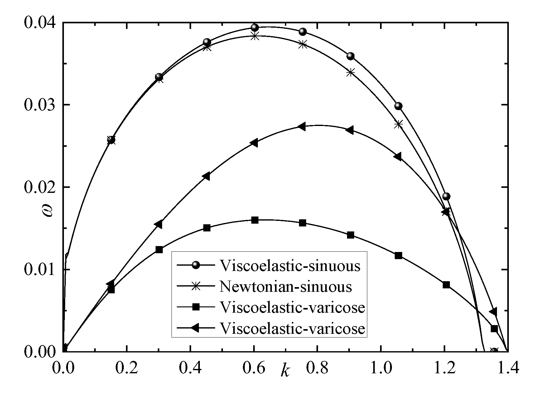
Figure 3 illustrates the dispersion relations for Oldroyd-B and Newtonian fluid sheets in the electric field under the sinuous and varicose modes. In both modes, the growth rates are greater when the sheet is a non-Newtonian fluid. The sheet becomes more unstable when non-Newtonian rheological properties are considered. In this sense, research on the instability of a viscoelastic liquid sheet could identify potential methods for breaking liquid sheets into droplets. Additionally, in the varicose mode, there is greater discrepancy between the two kinds of fluids. Overall, the sinuous mode plays a leading role in the sheet instability of the two fluids. However, the unstable areas are almost the same for both modes. The following sections analyze the effects of the physical properties of the sheet on its instability.

4.2. Electrical Properties

This section explores the influence of the electric field strength ($Eu,D$), the relaxation time of the surface charge ($\tau$), and electric permittivity ($\epsilon$) on the sheet instability.

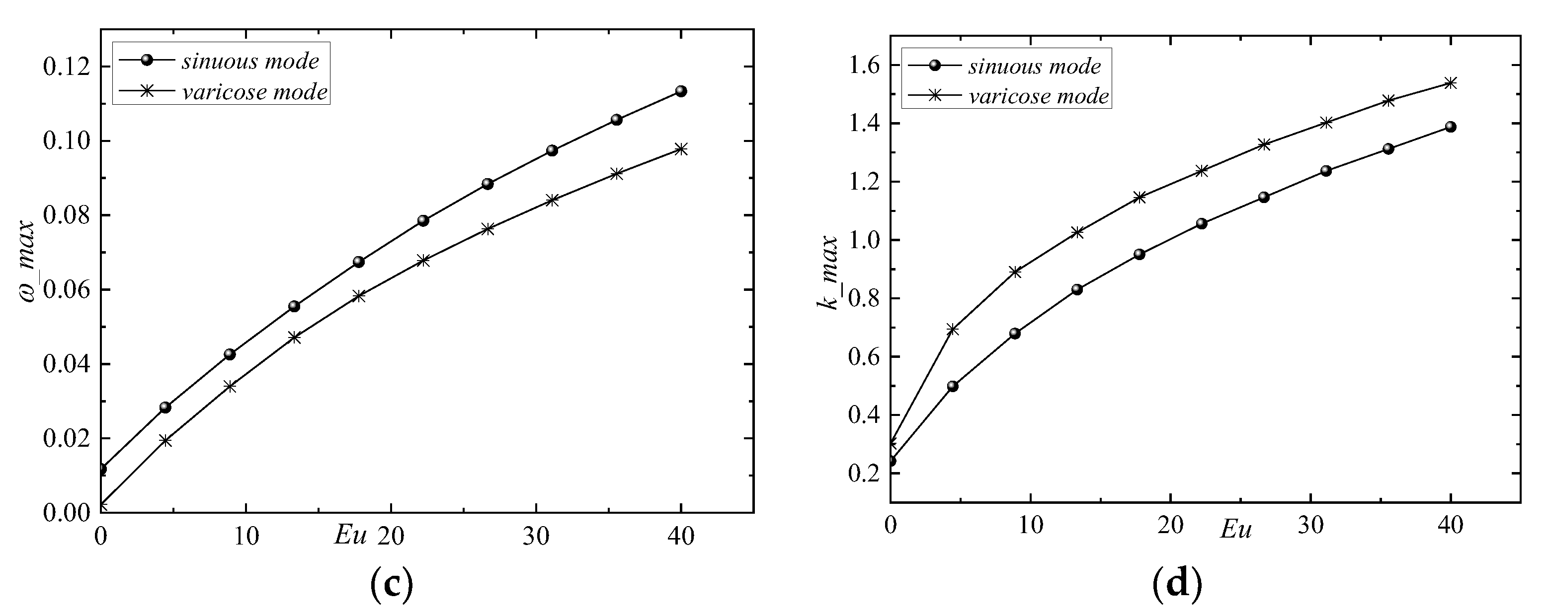
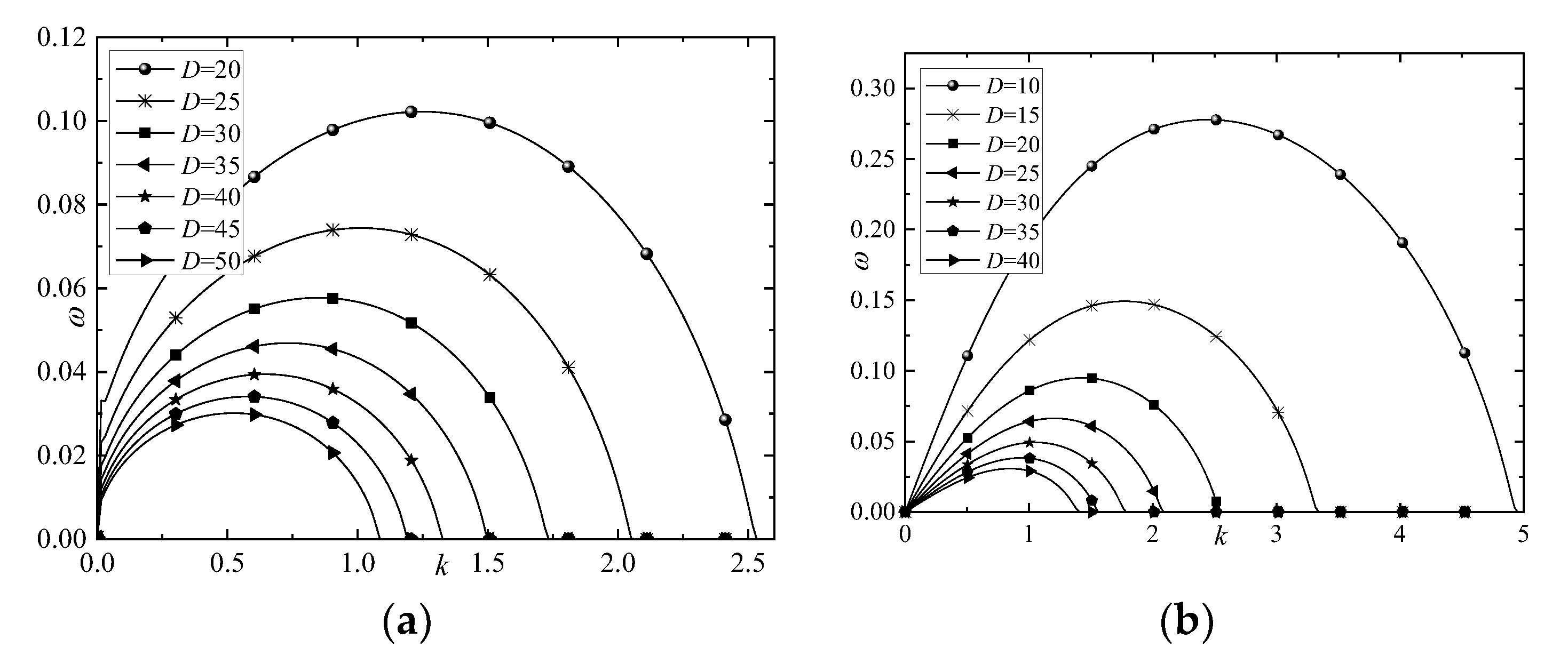
The effect of the electric strength $Eu$ on the sheet instability is depicted in Figure 4. It can be observed obviously that the electric strength causes the liquid sheet to become dramatically more unstable in both modes. Furthermore, the unstable range of the wavenumber widens as the electric strength increases. It can be seen that the maximum unstable growth rate for the sinuous mode is greater than that for the varicose mode, indicating that the sinuous mode plays a dominant role in the sheet instability. A liquid sheet with a larger maximum unstable growth rate can behave with greater instability. The dominant wavenumber is slightly larger in the varicose mode. According to the studies of Yin [21] et al., increasing the Eu can promote the breakup process and obtain a smaller main drop size.

The effect of the dimensionless distance $D$ on the instability of the viscoelastic liquid sheet is further studied in the present study, as shown in Figure 5. According to Equation (8), the electric strength increases sharply as $D$ decreases. In this situation, it is easy to conclude that the sheet could become much more unstable in both modes if the distance between the electrodes was decreased, as the unstable area would widen considerably (Figure 4). Note that the varicose mode is more sensitive to variations in $D$. In brief, the electrical force accelerates the sheet’s breakup. The mechanism is complicated because the sheet has been formulated using the leaky dielectric model. According to recent studies, decreasing the distance is beneficial to obtain a smaller main drop size after the breakup process. This is discussed in detail in Section 4.3.

The fluid conductivity is represented by the electrical relaxation time $\tau$ and the relative electrical permittivity $\epsilon$. In fact, the effects of $\tau$ and $\epsilon$ are limited, which has been reported in previous studies [23], because the two parameters only influence the conductive term of the surface charge conservation in Equation (13). Compared with the electrical relaxation time $\tau$, the relative electrical permittivity $\epsilon$ has a slightly greater effect because it is included in the electric field strength. As Figure 6 shows, enhancing $\epsilon$ causes the maximum growth rate ${\omega }_{\max }$ to increase. In this sense, the relative electrical permittivity is an unstable factor for a sheet.

4.3. Rheological Properties

This section explores the effect of the sheet rheological properties, including the elasticity and time constant ratio, on sheet instability.

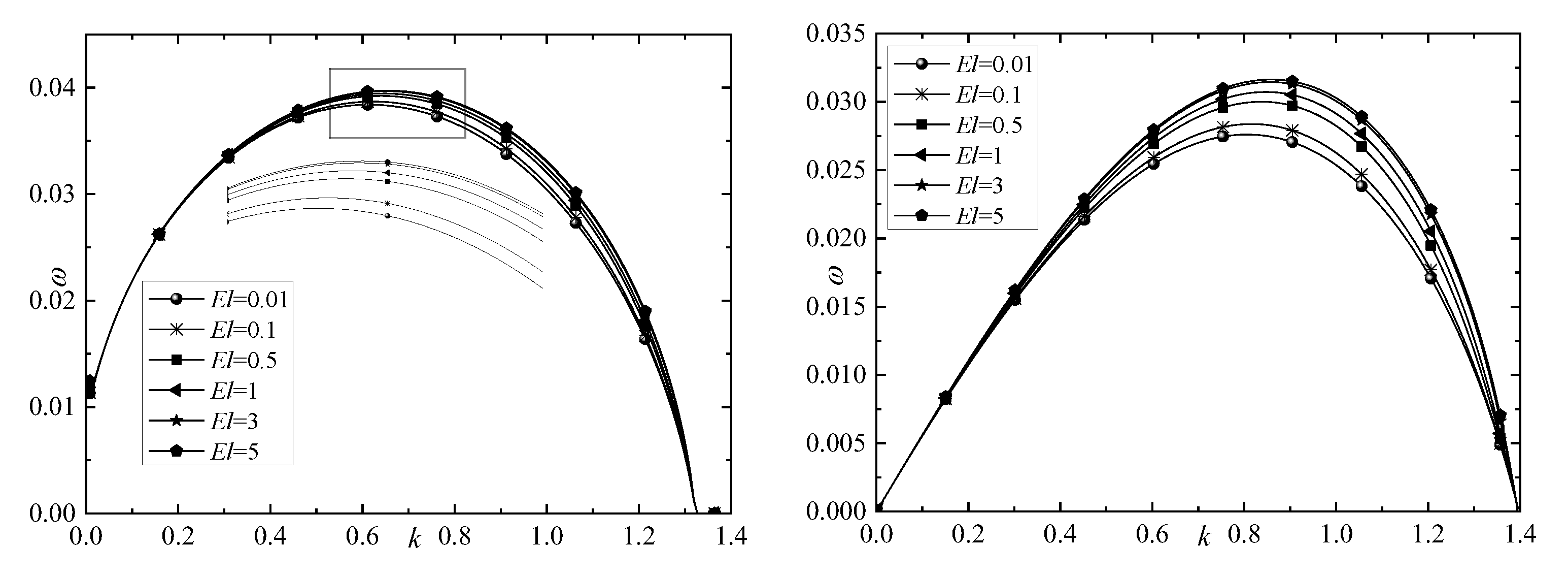
Liquid elasticity is an important parameter in the stability of the sheet. Figure 7 displays curves of the temporal growth rate varies with the wavenumber. It can be seen clearly that the temporal growth rate increases as the elasticity number increases. The results suggest that the elasticity has a destabilizing effect on the viscoelastic sheet. The effect of the elasticity number in the linear analysis can be explained by the equation in Table 2: increasing $El$ results in an increase in ${\lambda }_1$, leading to a larger effective Reynolds number. Figure 7 also shows that the temporal growth rate varies only slightly for different elasticity numbers, so the destabilizing effect of viscoelasticity is weak according to linear analysis. Further aspects of the mechanism of the elasticity number $El$ on the linear temporal growth rate $\omega$ are examined in Section 4.4.

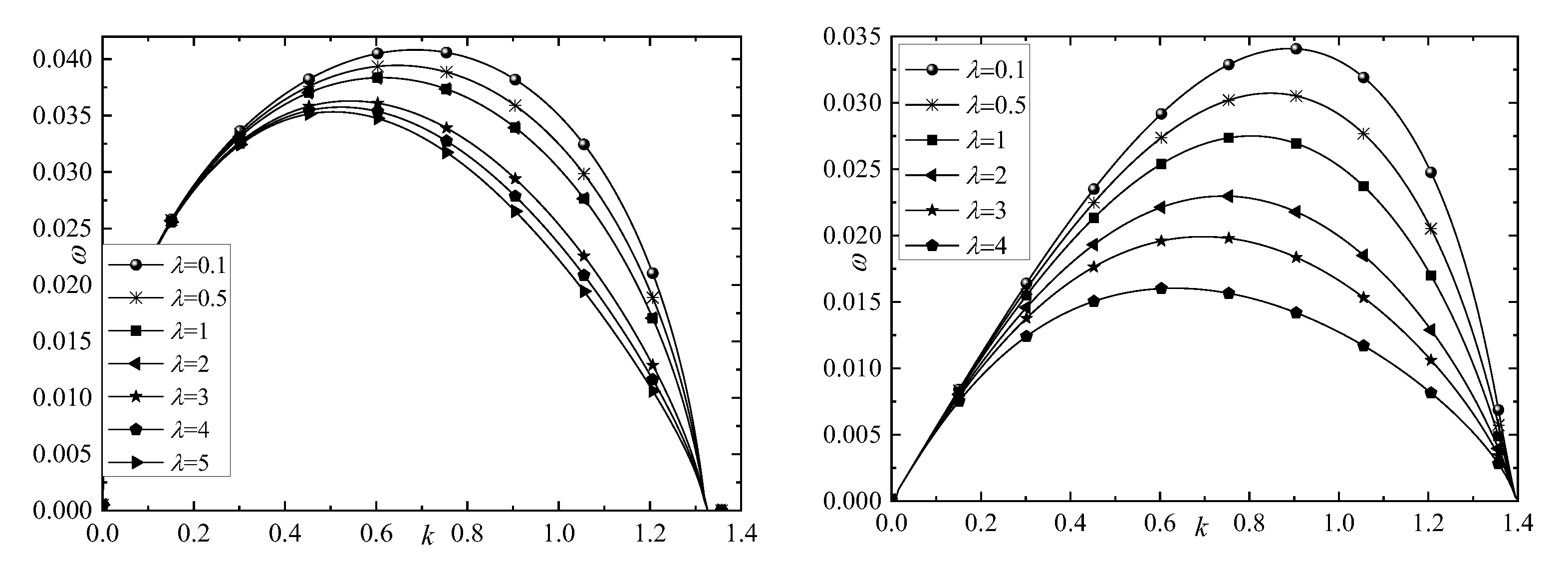
In the present study, the time constant ratio is defined as the ratio of the deformation retardation time ${\lambda }_2$ to the stress relaxation time ${\lambda }_1$. Figure 8 illustrates the effects of the time constant ratio on sheet instability under the sinuous and varicose modes, respectively. It can be seen obviously that the temporal growth rate decreases with an increasing time constant ratio. It means that the viscoelastic planar liquid sheet behaves with greater stability as the time constant ratio increases, i.e., decreasing the time constant ratio promotes the breakup process of the liquid sheet. Figure 8 also shows that the time constant ratio has a relatively large effect. As the stress tensor of a viscoelastic liquid sheet can be increased by enlarging the deformation retardation time ${\lambda }_2$, according to Equation (1), the liquid sheet will become more unstable. The effects of other properties, such as viscosity, surface tension, and density, are well-known [9,10,16], so a detailed description is omitted here.

4.4. Mechanism Analysis

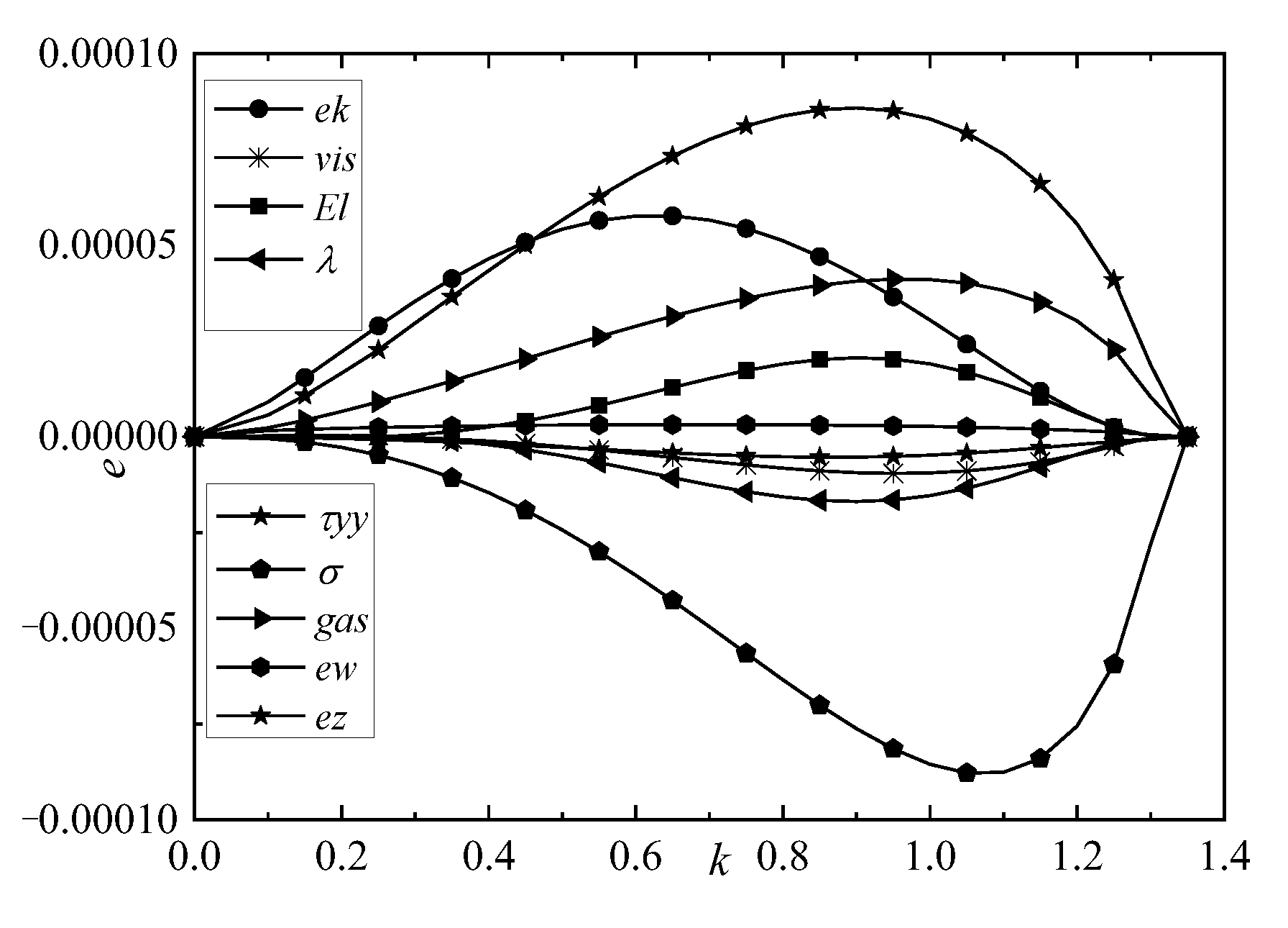
In this section, an energy budget is derived to explain the mechanism of the onset of instability. For the sinuous mode, the rates of change in the kinetic energy and various forces are shown as a function of the wavenumber at the onset of instability $\left(t=0\right)$ in Figure 9, according to Equation (39) in Section 3. Firstly, ${\dot{w}}_{ez},{\dot{w}}_{ew},{\dot{w}}_g,{\dot{w}}_{El}$ are positive, so the electrical strength, ambient gas, and elasticity have a destabilizing effect, which explains the trend in the temporal growth rate identified in Section 4.2 and Section 4.3. In contrast, ${\dot{w}}_{\overline{\lambda }},{\dot{w}}_{\sigma },{\dot{w}}_{vis}$ are negative, so deformation retardation, surface tension, and viscosity have a stabilizing effect. This explains the phenomenon observed in Section 4.3, whereby an increase in the time constant ratio $\overline{\lambda }$ reduces the temporal growth rate $\omega$. Additionally, ${\dot{w}}_{\tau yy}$ is very small, but positive, so it slightly destabilizes the sheet. Secondly, the absolute values of ${\dot{w}}_{\sigma },{\dot{w}}_{ez}$ are much greater than those of the other forces, so the electric force and aerodynamic force dominate the sheet instability. The magnitudes of ${\dot{w}}_{\overline{\lambda }},{\dot{w}}_g,{\dot{w}}_{El}$ are also considerable, so they are secondary factors in the instability of the viscoelastic sheet.

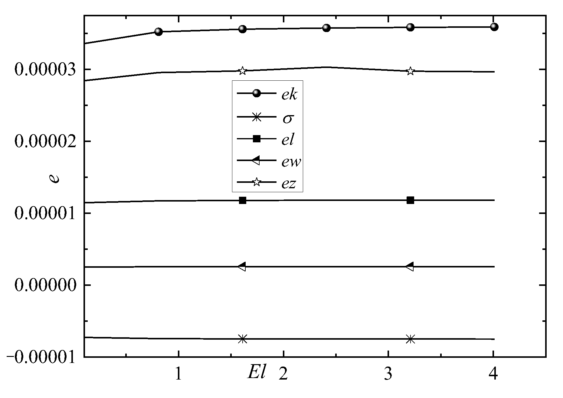
The present study focuses on the influence of viscoelasticity and electric strength on instability, so the effects of the elasticity number $El$, time constant ratio $\overline{\lambda }$, and electrical Euler number $Eu$ are further examined in Figure 10, Figure 11 and Figure 12. Generally, the rates of all forces exhibit minor variations with respect to the elasticity number, as shown in Figure 10. As the elasticity number increases, ${\dot{w}}_{ez},{\dot{w}}_{ew},{\dot{w}}_{El}$ increase, whereas ${\dot{w}}_{\sigma }$ decreases slightly, but the absolute value of the rate of change in kinetic energy increases, which means that the force created by elasticity does more work to enhance the instability as the elasticity increases. However, this provides a limited explanation for the effect of elasticity on the temporal growth rate shown in Figure 6, whereby $\omega$ increases slightly as $El$ increases.

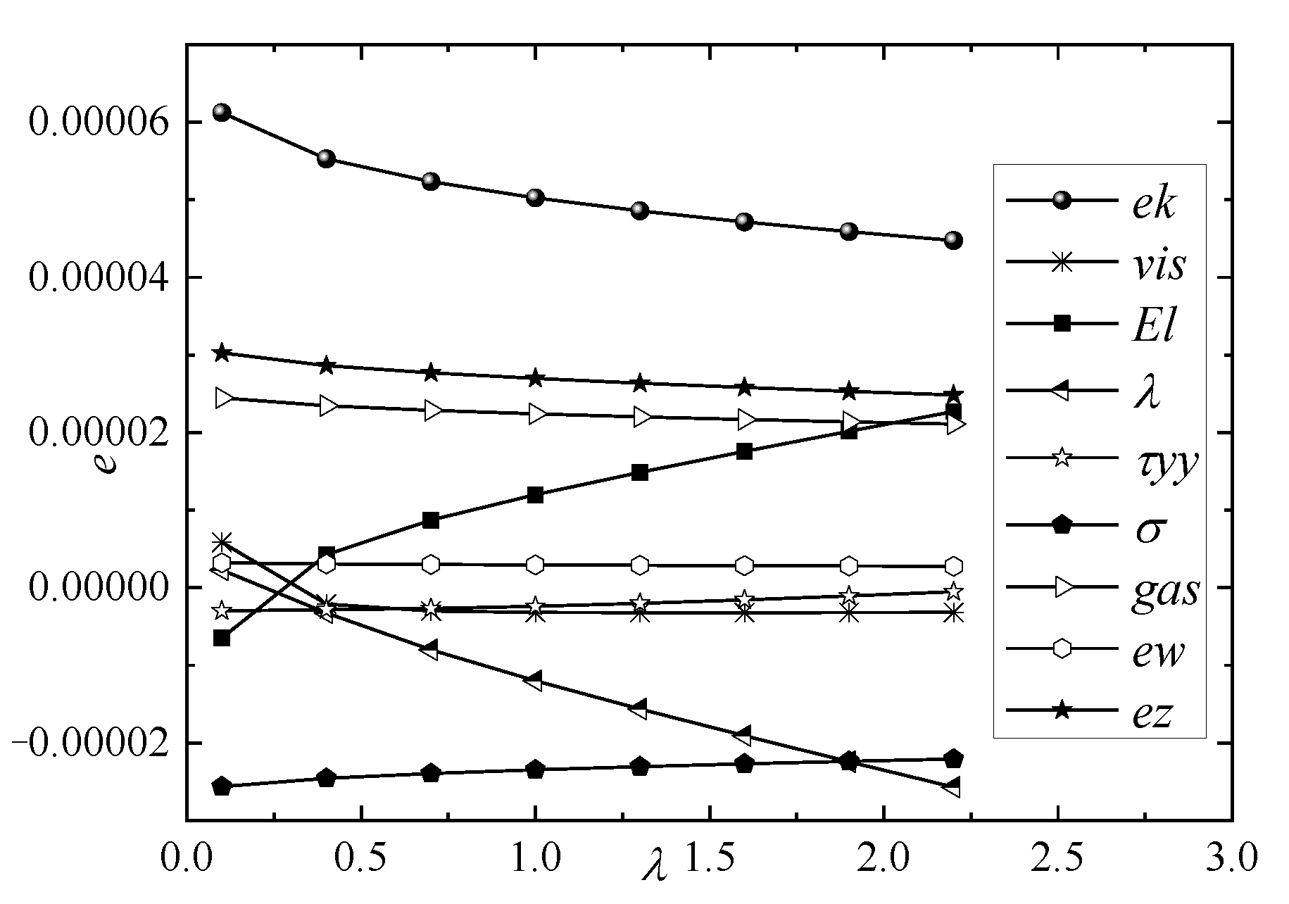
The effect of the time constant ratio $\lambda$ is shown in Figure 11. The kinetic energy and other forces vary considerably as $\lambda$ changes. Firstly, as $\lambda$ increases, ${\dot{w}}_{El},{\dot{w}}_{\sigma }$ increase while ${\dot{w}}_{ez},{\dot{w}}_g,{\dot{w}}_{\overline{\lambda }}$ decrease. The other forces remain basically unchanged. Note the significant change in the kinetic energy, which implies that the time constant ratio effectively enhances the sheet instability, as shown in Figure 7. Secondly, increasing the time constant ratio weakens the effect of the electric force. Finally, as $\lambda$ increases, ${\dot{w}}_{El}$ increases markedly, whereas ${\dot{w}}_{\overline{\lambda }}$ decreases rapidly. The elasticity enhances the instability, but is not sufficient to compensate for most of the energy dissipated by deformation retardation. As a result, the time constant ratio stabilizes the sheet.

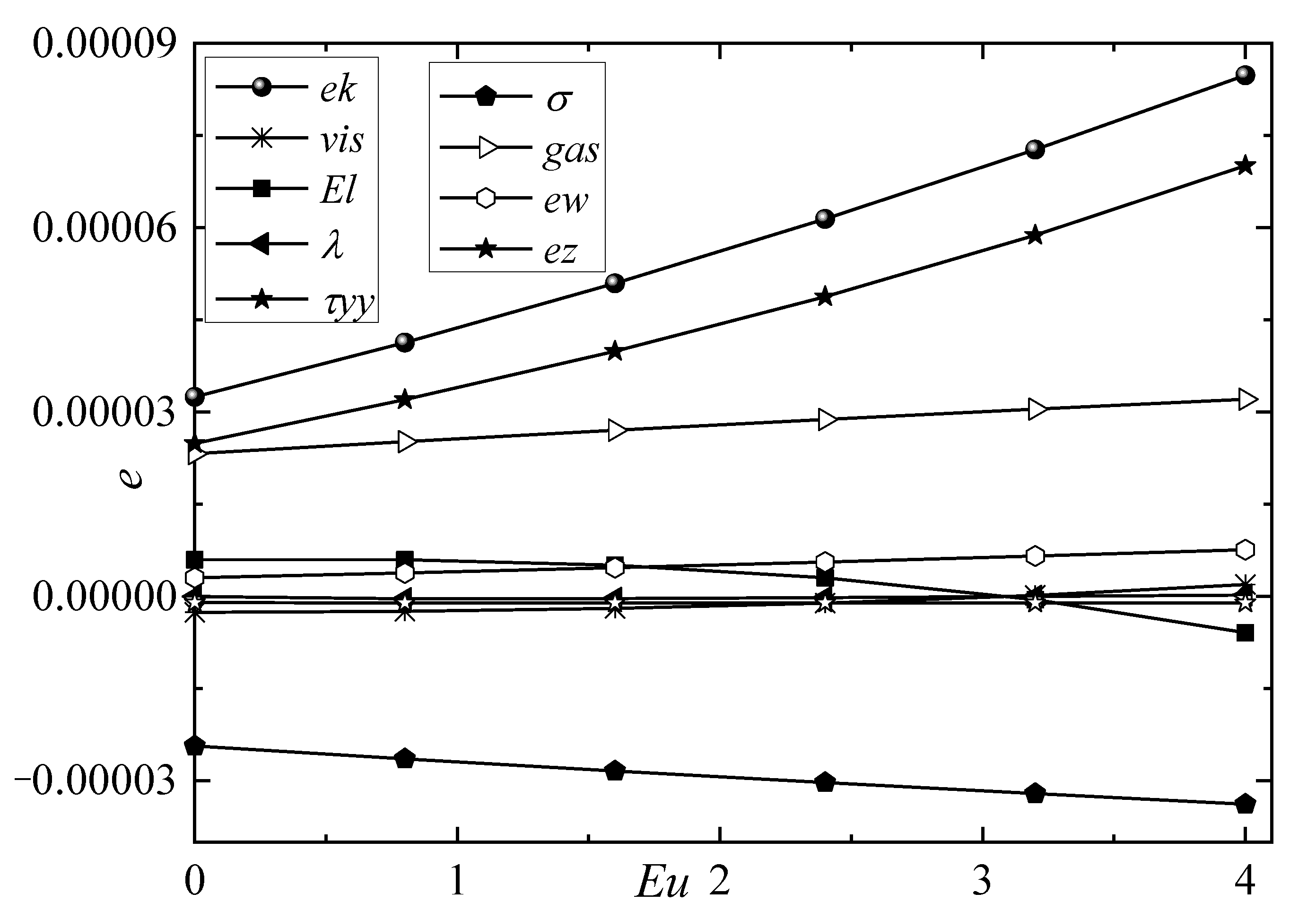
Figure 12 displays the effect of the electrical Euler number $Eu$ on the rate of change in the kinetic energy and other forces. When $Eu$ increases, the ${\dot{w}}_{ez},{\dot{w}}_g$ increase, while ${\dot{w}}_{El},{\dot{w}}_{\sigma }$ decrease. Note that ${\dot{w}}_{ez}$ grows rapidly as $Eu$ changes, resulting in the kinetic energy increasing dramatically. Thus, the electric force is a leading factor in the instability of the sheet, as illustrated by Figure 4. It is worth noting that ${\dot{w}}_{El}$ decreases markedly as $Eu$ increases, which reduces the destabilizing effect of the liquid elasticity on the sheet. In this sense, the effect of surface tension has been enhanced.

5. Conclusions

The present study made two main contributions. Firstly, using temporal linear analysis, the instability of a non-Newtonian liquid sheet moving through inviscid gas in a transverse electrical field was studied with the leaky dielectric model. Secondly, an energy budget was used to investigate the mechanism of sheet breakup. The results presented herein explained the interaction between the electric field and the rheological properties.

The electric field strength and liquid elasticity caused the liquid sheet to be dramatically unstable in both sinuous and varicose modes. Furthermore, the unstable range of the wavenumber widened as the electric strength increased. A viscoelastic planar liquid sheet behaved with greater stability as the time constant ratio increased.

According to the energy budget, the aerodynamic forces, electrical forces, and liquid elasticity enhanced the sheet instability by doing positive work, whereas the surface tension, viscous stresses, and deformation retardation performed negative work, indicating their stabilizing effects. The electrical force was the most significant destabilizer of the sheet under the leaky dielectric model. Additionally, increasing the time constant ratio weakened the effect of the electric force, while the electric force could reduce the destabilizing effect of liquid elasticity on the sheet.

References

- Lefebvre, A.H.; Wang, X.F.; Martin, C.A. Spray characteristics of aerated-liquid pressure atomizers. J. Propuls. Power 1988, 4, 293–298. [Google Scholar] [CrossRef]
- Lefebvre, A.H. Atomization and Sprays; CRC Press: New York, NY, USA, 1989. [Google Scholar] [CrossRef]
- Ahmadi, M.; Sellens, R.W. A simplified maximum-entropy-based drop size distribution. At. Sprays 1993, 3, 291–310. [Google Scholar] [CrossRef]
- Bayvel, L.; Orzechowski, Z. Liquid Atomization; Taylor and Francis: Washington, DC, USA, 1993; ISBN 9780891169598. [Google Scholar]
- Squire, H.B. Investigation of the Instability of a Moving Liquid Film. Br. J. Appl. Phys. 1953, 4, 167–169. [Google Scholar] [CrossRef]
- Hagerty, W.W.; Shea, J.F. A study of the stability of plane fluid sheets. J. Appl. Mech. 1955, 22, 509–514. [Google Scholar] [CrossRef]
- Melcher, J.R. Field-Coupled Surface Waves: A Comparative Study of Surface-Coupled Electrohydrodynamic and Magnetohydrodynamic Systems; MIT Press: Cambridge, MA, USA, 1963. [Google Scholar]
- Melcher, J.R.; Schwarz, W.J., Jr. Interfacial Relaxation Overstability in a Tangential Electric Field. Phys. Fluids 1968, 11, 2604. [Google Scholar] [CrossRef]
- El-Sayed, M.F. Electro-Aerodynamic Instability of a Thin Dielectric Liquid Sheet Sprayed with an Air Stream. Phys. Rev. E 1999, 60, 7588–7591. [Google Scholar] [CrossRef]
- Yang, L.J.; Liu, Y.X.; Fu, Q.F.; Wang, C. Linear Stability Analysis of Electrified Viscoelastic Liquid Sheets. At. Sprays 2012, 22, 951–982. [Google Scholar] [CrossRef]
- Melcher, J.R.; Taylor, G.I. Electrohydrodynamics: A review of the role of interfacial shear stresses. Annu. Rev. Fluid Mech. 1969, 1, 111–146. [Google Scholar] [CrossRef]
- Saville, D.A. Electrohytrodynamics: The Taylor–Melcher Leaky Dielectric Model. Annu. Rev. Fluid Mech. 2003, 29, 27–64. [Google Scholar] [CrossRef]
- Cimpeanu, R.; Papageorgiou, D.T.; Petropoulos, P.G. On the Control and Suppression of the Rayleigh–Taylor Instability Using Electric Fields. Phys. Fluids 2014, 26, 022105. [Google Scholar] [CrossRef]
- Savettaseranee, K.; Papageorgiou, D.T.; Petropoulos, P.G.; Tille, B.S. The effect of electric fields on the rupture of thin viscous films by van der Waals forces. Phys. Fluids 2003, 15, 641–652. [Google Scholar] [CrossRef]
- Tilley, B.S.; Petropoulos, P.G.; Papageorgiou, D.T. Dynamics and rupture of planar electrified liquid sheets. Phys. Fluids 2001, 13, 3547. [Google Scholar] [CrossRef]
- Liu, Z.; Günter, B.; Durst, F. Linear analysis of the instability of two-dimensional non-Newtonian liquid sheets. J. Non-Newton. Fluid Mech. 1998, 78, 133–166. [Google Scholar] [CrossRef]
- Brenn, G.; Liu, Z.; Durst, F. Three-dimensional temporal instability of non-Newtonian liquid sheets. At. Sprays 2001, 11, 49–84. [Google Scholar] [CrossRef]
- Jia, B.Q.; Xie, L.; Yang, L.J.; Fu, Q.F.; Cui, X. Linear instability of viscoelastic planar liquid sheets in the presence of gas velocity oscillations. J. Non-Newton. Fluid Mech. 2019, 273, 104169. [Google Scholar] [CrossRef]
- Oldroyd, J.G. On the Formulation of Rheological Equations of State. Proc. R. Soc. Lond. Ser. A 1950, 200, 523–541. [Google Scholar] [CrossRef]
- Oldroyd, J.G. Non-Newtonian Effects in Steady Motion of Some Idealized Elastico-Viscous Liquids. Proc. R. Soc. Lond. A 1958, 245, 278–297. [Google Scholar] [CrossRef]
- Li, F.; Yin, X.Y.; Yin, X.Z. Axisymmetric and non-axisymmetric instability of an electrically charged viscoelastic liquid jet. J. Non-Newton. Fluid Mech. 2011, 166, 1024–1032. [Google Scholar] [CrossRef]
- Weder, M.; Gloor, M.; Kleiser, L. Decomposition of the temporal growth rate in linear instability of compressible gas flows. J. Fluid Mech. 2015, 778, 120–132. [Google Scholar] [CrossRef] [Green Version]
- Ruo, A.C.; Chen, K.H.; Chang, M.H. Instability of a charged non-Newtonian liquid jet. Phys. Rev. E 2012, 85, 016306. [Google Scholar] [CrossRef]
- Carroll, C.P.; Joo, Y.L. Electrospinning of viscoelastic Boger fluid: Modeling and experiments. Phys. Fluids 2006, 18, 053102. [Google Scholar] [CrossRef]
Figure 1.
Schematic diagram of moving liquid sheet in an electric field.
Figure 2.
The figure of the liquid sheet “varicose” and “sinuous” modes.
Figure 3.
Temporal instability of an Oldroyd-B and Newtonian fluid sheet in the electric field for sinuous and varicose modes.
Figure 4.
Effects of on (a) sheet instability for sinuous mode, (b) sheet instability for varicose mode, (c) maximum growth rate, and (d) dominant wavenumber.
Figure 5.
Effects of on sheet instability for (a) sinuous mode and (b) varicose mode.
Figure 6.
Effects of on sheet instability for sinuous and varicose modes.
Figure 7.
Figure 8.
Figure 9.
Rates of change in kinetic energy and various forces for sinuous mode.
Figure 10.
Effect of elasticity number on the rate of change in the kinetic energy and other forces.
Figure 11.
Effect of time constant ratio on rate of change in the kinetic energy and other forces.
Figure 12.
Effect of electrical Euler number on rate of change in kinetic energy and other forces.