
Tensor of Order Two and Geometric Properties of 2D Metric Space

1
Department of Production Systems and Robotics, Faculty of Mechanical Engineering, The Technical University of Kosice, Letná 9, 04001 Košice, Slovakia
2
Department of Applied Mathematics and Informatics, Faculty of Mechanical Engineering, The Technical University of Kosice, Letná 9, 04001 Košice, Slovakia
*
Author to whom correspondence should be addressed.
Mathematics 2022, 10(19), 3524; https://0-doi-org.brum.beds.ac.uk/10.3390/math10193524
Submission received: 9 August 2022
/
Revised: 4 September 2022
/
Accepted: 21 September 2022
/
Published: 27 September 2022
(This article belongs to the Section Engineering Mathematics)
Abstract
:A 2D metric space has a limited number of properties through which it can be described. This metric space may comprise objects such as a scalar, a vector, and a rank-2 tensor. The paper provides a comprehensive description of relations between objects in 2D space using the matrix product of vectors, geometric product, and dot product of complex numbers. These relations are also an integral part of the Lagrange’s identity. The entire structure of derived theoretical relationships describing properties of 2D space draws on the Lagrange’s identity. The description of how geometric algebra and tensor calculus are interconnected is given here in a comprehensive and essentially clear manner, which is the main contribution of this paper. A new term in this regard is the total geometric and matrix product, which—in a simple manner—predetermines and defines the existence of differential relations such as the gradient, the divergence, and the curl of a vector field. In addition, geometric interpretation of tensors is pointed out, expressed through angular parameters known from the literature as a tensor glyph. This angular interpretation of the tensor has an unequivocal analytical form, and the paper shows how it is linked to the classical tensor denoted by indices.
MSC:
15A60; 15A67; 15A69; 15A721. Introduction
The mash of different mathematical fields is made of independent mathematical streams functioning next to each other as parallel worlds. This comparison is somewhat lame, as there also must be a clearly demonstrated interconnection between those streams, something that cannot be said of parallel worlds. It can be assumed that this interconnection is most illustrative if interpreted geometrically. This paper’s task is to point out the comprehensive construction of various known space-describing algebra, with a common factor running through. This common factor is the Lagrange’s identity, expressed in its simplest form through four input elements.
Various means can be employed to describe space. At around 1636, French mathematicians René Descartes and Pierre de Fermat founded analytical geometry through identifying solutions to an equation with two variables with points on a planar curve [1].
The first hint of the term vector space may be found in the work titled “Die lineale Ausdehnungslehre, ein neuer Zweig der Mathematik by Hermann Grassmann” from 1844 [2]. However, his work remained mostly in obscurity because Grassmann was not a professional mathematician, and he was describing his theory in a philosophical manner. The exterior algebra created by Grassmann is an algebraic system, the result of which is an outer product. The exterior algebra provides an algebraic space that makes it possible to answer geometric questions. Clifford defined a new algebra, in which the product is demonstrated as a unification of the Grassmann algebra and the Hamilton quaternion algebra. This is how the foundations of geometric algebra were laid. Clifford algebra provides the grammar. Complex number, quaternions, matrix algebra, vector, tensor and spinor calculus, and differential forms are integrated into a single comprehensive system [3].
At present, geometric algebra is experiencing a sort of renaissance because it started to be intensely used in the last decades only. There are a number of different ways to define geometric algebra. Some works define the Clifford algebra as the multiplication of vectors in R2 [4,5,6,7]. In that case, the outer and inner product are defined as the basic equation of geometric algebra. This formalism is used to define Clifford spaces. The Clifford algebra can also be defined using the quadratic form [8,9]. This is how various Clifford algebras are created, some of which are used to describe physical phenomena. In a more abstract form, the definition is based on the axiomatic principle [3,10]. The basis is the definition of four vectors in the Clifford algebra marked Cl 1,3 (R). This algebra is referred to as spacetime algebra and is suitable as a description of relativistic physics. Some works are focused on the application of geometric algebra in various other algebras. For example, ref. [11] gives a full classification of Lie algebras of specific type in complexified Clifford algebras. Geometric algebra provides a new formalism for differentiation on vector manifolds and for mappings between surfaces, including conformal mappings [12]. The following works are already focused on the application of geometric algebra in physical relationships. For example, ref. [13] aimed at a better description of the power theory of electrical phenomena using geometric algebra. Article [14] aimed at a compact description of electrical relationships via geometric algebra used in the field of electrical engineering. Article [15] used conformal geometric algebra to improve imaging methods in medicine. Similarly, geometric algebra is also used for visualization in the field of crystallography [16].
The tensor calculus was developed in about 1890 by G. Ricci-Curbastro under the name of an absolute differential calculus, and Ricci-Curbastro first introduced it in 1892. It became accessible to many mathematicians through publication of the classical text of Ricci-Curbastro and Tullio Levi-Civita in 1900 as “Méthodes de calcul différentiel absolu et leurs applications” (Methods of the absolute differential calculus and their applications) [17].
Description of spatial properties constitutes a subject matter with well-explored theory. That is why research focused on application areas of using the tensor calculus, geometric algebra, and complex numbers. Some works are focused on the application of tensor calculus in the description of the dynamics of a mechanical object. In robotics, the calculation methodology using the inertia tensor has been improved [18]. The work [19] contains a description of the metric tensor on a Riemannian manifold. The analysis provides optimization of the dynamic parameters of the robotic arm. Tensors are also a good tool for the analysis of complex systems such as turbulent flow. Article [20] provides a rigorous and well-documented description of a mathematical and computational framework that can be used for the calculation of the structure tensors in arbitrary turbulent flow configurations. Other works are aimed at the further development of tensor calculus, for example, a special method of higher-order tensor decomposition based on the similarity of matrix decomposition [21] or a new method to produce lower bounds for the Waring rank of symmetric tensors [22]. New perspectives are also provided by the field of Riemannian metrics. For example, work [23] focused on the concept of quasi-semi-Weyl structure, and we provide a few ways for constructing quasi-statistical and quasi-semi-Weyl structures by means of a pseudo-Riemannian metric, affine connection, and tensor field on a smooth manifold.
This historical context points to a substantial development in the area of describing space and its properties. Recently, thanks to numerical methods, works that try to make the object of tensor more visible through numerical methods, calling it a tensor glyph, have started to crop up.
A tensor glyph displays multidimensional data using several possible rules [24]. The main use is in the visualization of fluid dynamics tensors, tension tensors or the Jacobian of the velocity field [25]. Nowadays, tensor glyphs are fully used for visualization in the field of medicine with magnetic resonance [26,27,28]. Various forms of displaying tensor glyphs exist. An analytical method of tensor glyph display has not yet been developed. All methods are based on the application of numerical procedures. In some works, Mohr diagrams are used to display the stress tensors [29]. A certain possibility is the use of superquadratic tensor glyphs [30,31]. This method is only suitable for symmetric tensors. Tensor visualization research also explores the use of different space metrics such as Frobenius, Euclidean, Wasserstein, and Fisher Rao [32].
The focus of our paper falls on a new approach to space description. It draws on topological concept of space described by the Lagrange’s identity. Nevertheless, this identity also meets the description of a metric space. That is why Lagrange’s identity takes the center stage in different algebra applications. Taking into account congruent transformation properties, it appears that space may be described—depending on its dimension—through only a limited number of parameters [33].
2. Description of 2D Space Using the Lagrange’s Identity
It is useful to start defining the interconnection between geometric space and tensors by defining spatial properties of the space itself. We will present the spatial characteristics in a somewhat non-traditional way, using the well-known Lagrange’s identity. The simplest form of Lagrange’s identity is the so-called four-square identity, dating all the way back to a Greek mathematician Diophantus from Alexandria (third century A.D.). Let be countable elements of any set. Then, the form of the Lagrange’s identity will be as follows:
This identity has its structure, which determines its specific properties. While it is true that the types of numbers that can be substituted for the identity elements are not specified, the identity operates with addition, multiplication, and exponentiation. All these operations may be matched by opposite operations such as subtraction, division, and square root. In the light of this fact, the identity involves all algebraic operations, so the domain of identity may correspond to the complex numbers domain.
2.1. Relation between Lagrangian Identity and Space
The left side of Lagrange’s’s identity can be linked to the common countable property of shared space. It can also be a topological space where the distance is not defined. Then, Lagrange’s’s identity may also be viewed as a form of transformation of elements into a new space. The mixed product of elements on the right side creates four new elements on the left side of the identity, which are, in a sense, a transformation of the original elements. This operation may be written as follows:
New elements will be of main importance in drawing the links between various multiplications of vectors.
Thanks to two distinct forms of modifying of the expression, the Lagrange’s identity takes two possible forms.
The first form is
The second form is
In literature, the second, less-known form is called the Brahmagupta–Fibonacci identity. The proof can be given by adding and subtracting in the following way:
Coefficients of the right side of the Lagrange’s identity or, alternatively, appear in the form of the Pythagoras theorem. It can also be shown that the ratios of the are independent of the ratio of the . A metric space can be created from these coefficients.
The Pythagoras theorem may be extended to higher dimensions of space, to which spatial Pythagoras theorem applies. The coefficient represents the spatial hypotenuse, and the other components are the legs of a right triangle. The following holds:
Similarly, the Lagrange’s identity, too, extends its applicability to higher dimensions of space. Generally, the Lagrange’s identity is expressed in the form below and may be used for description of spaces with higher dimensions.
2.2. Transformation Relations between the Left and Right Sides of the Lagrange’s Identity
Three independent elements suffice to describe a plane. The Lagrange’s identity is determined by four independent elements. It is, therefore, necessary to examine to what degree a transformation in the form of the Lagrange’s identity is reversible.
Theorem 1.
Letbe the four input elements of the left side of the Lagrange’s identity. Then, from the output elements, which are obtained on the right side of the Lagrange’s identity, a unequivocal back transformation to the original input elements cannot be performed.
Proof of Theorem 1.
Let us assume that we know the
elements, and we want to reverse determine the input elements of . We can proceed as follows. From Equations (2)–(4), we obtain
Further adjustments yield equations of ratios:
For an undisputed reverse determination of input elements, one more independent equation is still missing between elements and . Reverse transformation is not possible. □
Having arbitrarily selected value of an element, the above equations make it possible to additionally compute other elements. That is why reverse reconstruction of the transformation is possible only partially. Symbolically, the following holds:
3. Congruent Transformations in the Plane
Congruent transformations in the plane are those of an object rotation, translation, and reflection. The Lagrange’s identity describes a metric space, which is why it is possible to find a relationship between congruent transformations and the identity. Since the plane is unequivocally determined by three parameters, the object that is a part of the plane must also have three independent parameters so that individual congruent transformations can be distinguished on it. An object may be, e.g., a triangle defined by three points, a vector and a point constituting a triangle, or two non-parallel vectors anchored in the coordinate system‘s origin. The last example may also be expressed by two complex numbers in a complex plane. Thus, complex numbers operations yield the same results as vector operations.
Linear vector space is defined by linear operations only. These operations enable translation and scaling. Rotation and reflection cannot be done through linear operations. That is why vector space must be extended by the operation of mutual vector multiplication. Depending on the type of multiplication, a space with dot product is obtained (a unitary space), or in the case of a vector product, the resulting space is that with Lie algebra. The last extended spaces’ general properties of linear vector space by adding the possibility of rotation and reflection. The Lagrange’s identity has four independent input elements, which are multiplied by each other. That is why it can be assumed that the identity is in some form related to the transformation by rotation or reflection.
There are three known options of vector multiplication, and dual principle of interpretation of the multiplication result can be applied to all three cases. This is a matrix multiplications of vectors, which leads to dyadic vector product, geometric vector product, and finally dot product of complex numbers, where a complex number also represents a vector in a plane. Since dyadic vector product is also used in tensor calculus, it will be shown in what way the tensors are linked to multiplication of vector and how they are linked to the Lagrange’s identity, too.
In congruent transformations, the object maintains its size. The condition of object size maintenance, applying to various input elements, may be also transferred to the final value of the Lagrange’s identity. Based on this, in vector multiplication, a request may be made to keep a certain typical product characteristic under variable input elements. As will be shown, this condition of conservation the value defines a rank-2 tensor.
4. Description of 2D Space Using Matrix Multiplication of Vectors and Their Relation to Tensors and to the Lagrange’s Identity
For the sake of illustration, elements of the right side of the Lagrange’s identity will be used in all three product types.
Definition 1.
Let there be vectors defined asand. For the sake of coherence with the next chapter, the vectors are written in row form. This principle gives rise to the following two multiplication options. The product of a matrix with the size ofandyields a matrix with the size of
which is called a dot product of vectors.
Definition 2.
By changing the order of vector transposition, we obtain a matrix of the sizedetermined by the product of matrices of sizesand
This product is called a dyadic vector product. We mark it as the first form of dyadic product . In general, a product of matrices is not commutative, which is why it is advisable to interpret both multiplication options. Multiplication of yields the second form of dyadic product
5. Description of 2D Space Using the Geometric Product of Vectors and Relation to the Lagrange’s Identity
Geometric product of vectors originated from Clifford‘s work. Basic description of space constitutes Euclidean vector space defined by orthonormal bases . The geometric product of vectors is defined here in a new way based on the rules of multiplication of base vectors.
Definition 3.
Let two vectors of this space be defined asandand anchored in the origin. For the sake of obtaining the product of bases, arising from vector algebra of multiplying perpendicular and parallel vectors, inner and outer element multiplication is distinguished. Inner multiplication in the form ofis called a dot product and outer multiplication in the form of, a wedge product.
Products of identical base vectors
Products of perpendicular base vectors
Note.
Multiplication rules for base vectors are complemented with unused forms of the geometric product, where the product result is a zero. Unused forms do not affect the result of the geometric product; the process of solving the equation will only be clearer.
Geometric product is a linear combination of two types of multiplication in geometric algebra. However, various types of products cannot be added together. The wedge product is distinguished from the dot product by being marked as . This form of expressing the wedge product is not used in the literature but—as will be shown later—it is very significant in a conversion between individual types of multiplications of the input elements. In literature, the wedge product is referred to as a “blade”. In the case of 2D, this is a “bivector”. Linear combination of elements of different types of products gives rise to multivectors. The basic form of geometric product is a multivector, which consists of a scalar and a bivector on the equation’s right-hand side
Alternatively, when the order of vectors changes, the following applies
Geometric product corresponds to the sum of the elements from the right side of the first form of the Lagrange’s identity. By introducing vectors and , where the index means a changed order of the vector coordinates, the geometric product may be enhanced by the second form of the Lagrange’s identity expressed through the elements. This operation corresponds to the reflection of base of the vector space
By changing the order in which the vectors are multiplied, we obtain
Alternatively, the geometric product of vector and vector yields the following identities
Similarly, also
The Relationship between the Geometric Product and the Lagrange’s Identity
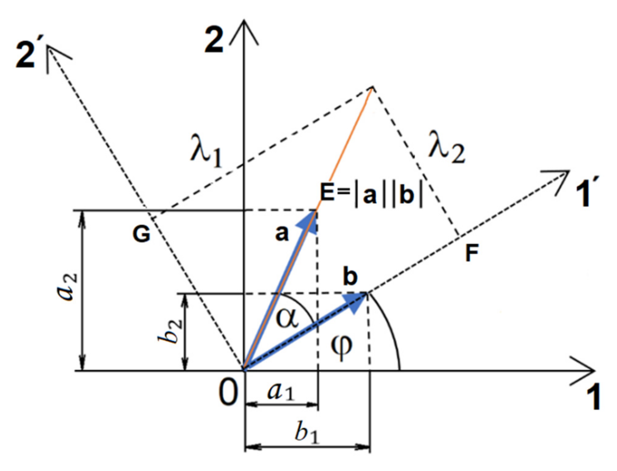
Geometric product incorporated in the Lagrange’s identity is expressed by the following equation:
The above equation has the form of the Pythagoras theorem. Then, the dot and the wedge vector product may be expressed through the angle , formed by the vectors according to the equations below.
Geometric equations are plotted on the graph in Figure 1.
6. Description of 2D Space Using the Dot Product of Complex Numbers and the Link to Geometric Product
In its essence, a complex number is a two-dimensional object. Direct multiplication of complex numbers under the distributive law yields a result, the form of which is, again, that of a complex number.
Multiplication of the complex numbers in the exponential form is commutative
where are real, non-negative constants. Multiplying two complex numbers in the algebraic form yields
Generally, however, a two-constituent element may be multiplied under a rule different than that of the distributive law applying to real numbers. In the case of complex numbers, the dot product of complex numbers may be used, too [34].
This product type is definitely used to solve spatial tasks because it is directly related to the Pythagoras theorem.
A new approach is that the multiplication procedure leads to a dual solution. That is why, unlike in the case of the usual representation of the dot product of complex numbers, a special multiplication sign is used.
Definition 4.
The dot product of complex numbers a, b in exponential form may be as follows:
whereis a sign for the planar product of complex numbers, while index 1 expresses a change of the first component into a complex conjugate. In the case of index 2, the second component of the product changes into a complex conjugate.
For the dot product of complex numbers in algebraic form, we obtain
alternatively, if the second number is replaced with a complex conjugate, we obtain
The following identities hold:
Note.
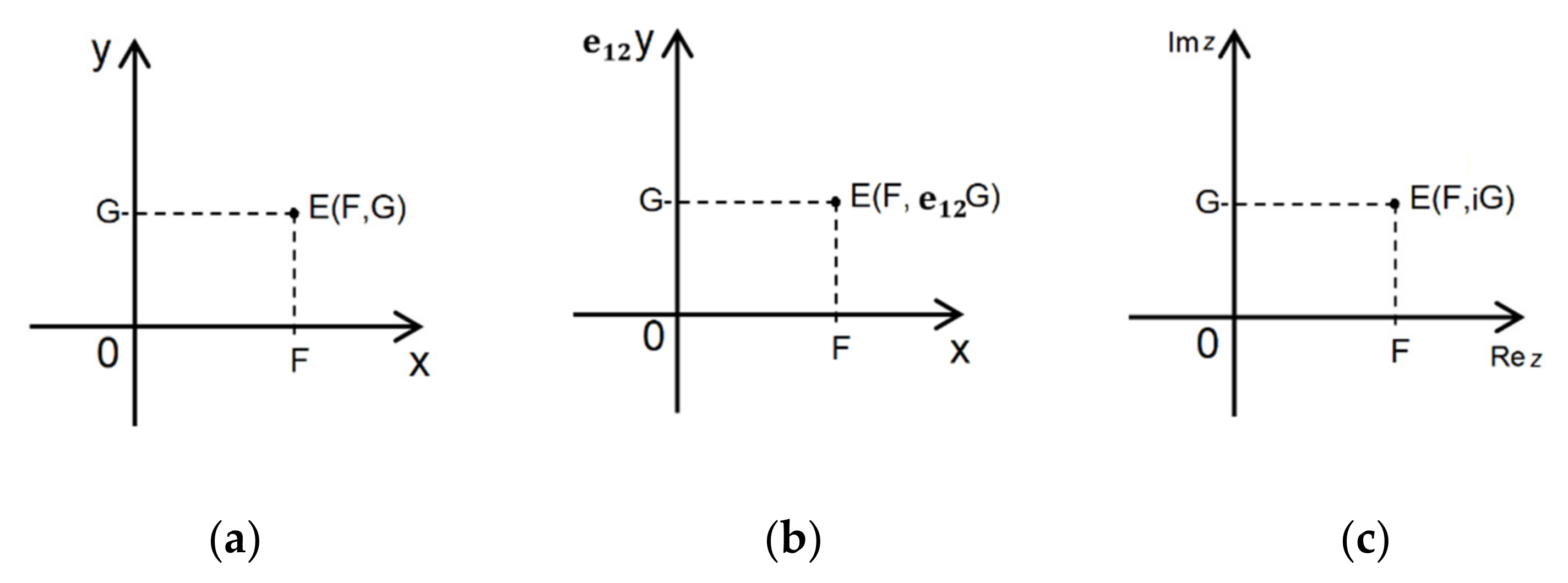
Complex numbers may be viewed as vectors having their initial point in the coordinate system’s origin. As can be seen, the dot product of complex numbers fully corresponds with geometric product of vectors as well as with the sum of theelements of the right side of the first form of the Lagrange’s identity. Through introduction of the vector space base reflection, equations can be derived also for theelements of the second form of the Lagrange’s identity. The only difference between the dot product of complex numbers and geometric product of vectors is the presence of an imaginary unit. This difference is similar to a difference between a complex and a real plane, as in the Figure 2. Formally, it can be asserted that designating the wedge product ascorresponds—as to its meaning—to the imaginary unit. However, to avoid misunderstanding, the imaginary unit in the case of a dot product of complex numbers is of a different nature than the one used in multiplying complex numbers. For example, squaring the imaginary unit yields the absolute value of the imaginary unit in this case
A plane created by the dot product of complex numbers is a complex plane, but the calculations differ.
7. Second Order Tensor Relationship with Different Forms of Vector Multiplication in 2D Space
There are essentially three ways to define a tensor, which reflect the chronological evolution of the notion through the last 140 years or so [35]:
- As a multi-indexed object that satisfies certain transformation rules,
- As a multilinear map,
- As an element of a tensor product of vector spaces.
The last two methods are independent of the coordinate system. However, for our purposes, the definition in the form of multi-indexed object is suitable. In general, a tensor is defined as multidimensional array. An nth-rank tensor in -dimensional space is a mathematical object that has indices and components and obeys certain transformation rules. Each index of a tensor ranges over the number of dimensions of space. This is a higher-order generalization of the fact that a 2-tensor, i.e., a linear operator, a bilinear form, or a dyad, can always be represented as a matrix [36]. Only second-order tensors with an orthonormal basis can have a relationship with various forms of vector multiplication since the result is bound to metric space. For these tensors, it is not necessary to distinguish between covariant and contravariant indices, and therefore, notation is possible in the following index form:
where is a second-order tensor; , are regular matrices; and is a second-order tensor with changed basis. In matrix form, it is
The matrices , are similar because the square matrix is regular. All similar square matrices that have the same Frobenian norm simultaneously have the same characteristic polynomial.
The outlined principle of tensor expression is used for generating all other tensor ranks. This means that, for example, it holds for rank 1 that a matrix of transformation exists from the first to the second base, which transforms the said vector. This vector is, at the same time, a rank-1 tensor.
where is a column vector expressed in the first base, and is one and the same vector expressed in the second base. Written in index form,
This principle of generating tensors of various ranks assumes that any arbitrary tensor and hence also a vector is invariant with respect to a change in the base. In this sense, a vector invariant can only be the vector’s size.
7.1. Description of Symmetric 2D Tensor and Relationship with Lagrange’s’s Identity
As mentioned above, different forms of vector multiplication are interconvertible using the right side of the Lagrange’s identity. Therefore, vector multiplication relations expressing a tensor will be convertible to all forms of vector multiplication. Taking the dyadic product creates a square matrix that can be used to describe the tensor.
A square matrix is a part of the same tensor if, upon a change in input parameters, it maintains its norm and invariants. The size of the matrix is characterized by the Frobenius matrix norm. If the matrix is to describe some congruent transformation, this norm should be constant. Invariants can be derived from the matrix characteristic polynomial
where is the identity matrix, and is a variable representing matrix eigenvalues. We determine the roots of the characteristic polynomial from the equation below.
Adjusting it, we obtain the following form:
where is the trace as the first invariant, and is determinant as the second tensor invariant. These invariants may also be expressed by means of input elements of Lagrange’s identity
Similarly, the determinant is zero also in the case of the second form of dyadic product . The trace has the following form:
The Frobenius norm for general matrix is in the following form:
where is the matrix transposed to matrix . Expression employing input elements has the following form:
Using the elements of the right side of the Lagrange’s identity, the norm results are in the following form:
It can by assumed from the last equation that a congruent transformation describes the component in the form of the matrix trace. Through transformation of rotation and reflection, a change in the base of vector space can be achieved. For example, if we want to express object reflection around the first coordinate axis, it is necessary to change the polarity of the second coordinate of the selected vector. Then, a vector in the form of , where the index denotes reflection, represents reflection around axis 1. Reflection also maintains the matrix norm, as is evidenced from the following equations:
As can be seen, all dyadic product components expressed through the matrix norm can be rewritten using the symbols of the right side of the Lagrange’s identity. That is why the same relationships apply to the reverse vector matrix product transformation as to the reverse transformation of the Lagrange’s identity. This proves the fact that reconstruction of original components is possible only partially, according to Theorem 1. This result speaks of the possibility to express tensors through dyadic product of two vectors, but an unambiguous reverse transformation is not possible. Thus, transformation equations written as a matrix apply only to right sides of the Lagrange’s identity and the dyadic product
Let the symmetric 2-tensor be defined generally by means of two-index elements, and let it be the result of some dyadic vector product. The symmetric matrix has the form of
where aij are input elements of the symmetric matrix. Roots of a characteristic polynomial of a symmetric tensor can be determined in the following way:
where is the identity matrix, and are eigenvalues of the matrix . The Frobenius norm of the symmetric matrix is in the following form:
7.2. Description of the General Tensor and Relationship with the Lagrange’s Identity
A general tensor, which emerged from dyadic product of vectors, is a sum of a symmetric and an skew-symmetric matrix. Components are now represented by two-index elements.
The degree of the general tensor asymmetry is expressed only by the element . If , then is a zero matrix, and the general tensor is, at the same time, a symmetric tensor.
To the skew-symmetric tensor , the following applies:
The value of is constant and independent of a change in the transformation parameter . Then the following must hold:
The transformed tensor will have the form below.
A sufficient condition for describing a plane is to have three parameters available. This condition is met by the symmetric tensor. In the case of a general tensor with four different parameters, the description is that of a curved space. The symmetric tensor does not enable an unambiguous reverse transformation to arrive at the original vector product elements either. However, a condition may be established determining the ratio of the input vector elements so that the result of dyadic product is a symmetric tensor. The following equation constitutes that condition:
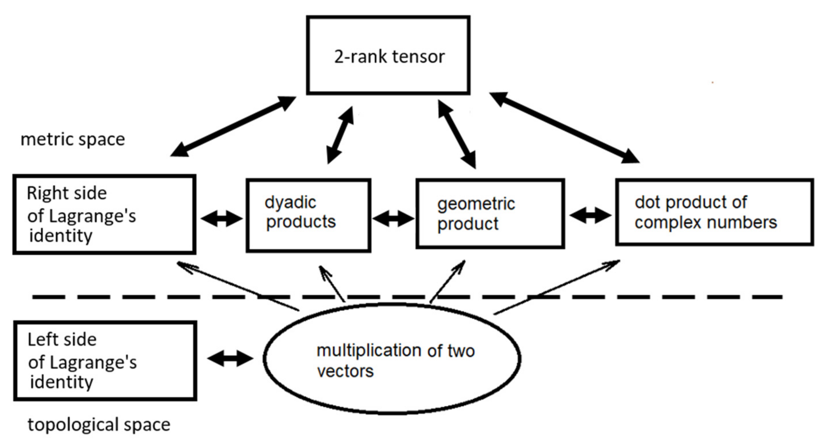
It can be derived from Equations (10) and (11) when . The Figure 3 below represents transformation options between individual mathematical entities.
8. Total Geometric and Matrix Product
In the case of geometric vector product and the dot product of complex numbers, each component was multiplied according to the rules of vector calculus. In the matrix vector product, vector components were considered to be only numbers, and vector calculus was not applied. However, on the other hand, the matrix vector product created all kinds of possible products between the input elements. By combining both multiplication types rules, a total geometric and matrix product can be created.
Definition 5.
Through different ordering of the transposed vector in the form of a sum of various products, a multivector emerges. Changing the order of multiplication of the input vectorsandgives rise to two possible forms.
First form
where the sign designates a total geometric and matrix product. Similarly, the second form of the total geometric and matrix product has the following form:
Since no other forms of multiplication exist, the matrix of the total geometric and matrix product may be considered a total tensor.
9. Differential Dependence of the Tensor Components
Gradient, divergence, and curl of a vector field are defined only for 3D space, using the vector product of vectors. The use of the geometric matrix product enables the definition of these concepts for other dimensions as well.
Definition 6.
Let several points in a plane compose a tensor field. If the value of the multivector, which includes a tensor, changes with the change of position of a point in metric space, the degree of change can then be expressed through derivation. In such case, the tensor is a function of the space variables. Derivation of the total rank-2 tensor in a plane defines a gradient of the tensor function.
The matrix part of the total tensor derivation is a tensor function gradient T
Definition 7.
The sum of the gradient elements with the dot product expresses divergence of the tensor function .
Definition 8.
The sum of the gradient components with the wedge product expresses the curl of the tensor function .
Note.
The equations above express the fundamental theorem of geometric calculus [37], which takes the form of
where if the geometric product, and it cannot be replaced with a gradient.
10. Visualization of 2D Space Properties Using Second-Order Tensors
Capturing a tensor through utilizing indices results in good computational properties, but it has a low degree of illustrativeness in terms of geometric rendering. In the case of a vector, the change in the base is carried out through a rotational matrix. Thus, there is a relative movement of the coordinate system with respect to the vector. The task may be reversed in a way in which the vector rotates, and the coordinate system remains unchanged. In such case, the geometric interpretation of the change in the vector’s end point position is a circle with the center lying in the origin. This is a relativistic view of tensor interpretation.
In the case of rank-2 tensors, the same interpretation philosophy may be applied. All maps of similar matrices elements constitute geometric interpretation of the tensor with respect to an unchanging coordinate system. The tensor is then expressed through angular parameters. In such case, the tensor is an omnidirectional geometric shape designated as a tensor glyph. If an angle of the coordinate system’s base rotation is marked graphically on such tensor, as it is in the Figure 1, then the angular tensor expression has the same information content as its notation by indices.
In the symmetric matrix case, it is necessary to verify transformational properties that guarantee the Frobenius norm value’s immutability. Eigenvalues , which constitute legs of a right triangle in the coordinate system, may be determined for any chosen symmetric matrix. The eigenvalues ratio may be expressed by the tangent of the angle , subtended between the vector and the positive part of the axis x
Then, the angle is typical for that tensor. When the base is rotated by angle , values of the matrix components change, but the angle remains. This means that the eigenvalues remain unchanged, and the matrix thus created corresponds to that same tensor.
Drawing on the knowledge of angle and the size of eigenvalues, elements of the matrix of rotated symmetric tensor can be computed. Tensor components may be calculated by applying the following formulae. For , the following holds true:
Derivation of equation is based on properties of symmetric tensor as described in the article [33]. One root of the quadratic equation represents the initial state and the second the state resulting from rotation by angle . For resolving the task, only the rotated state is interesting. Subsequently, other components of the rotated symmetric tensor are expressed
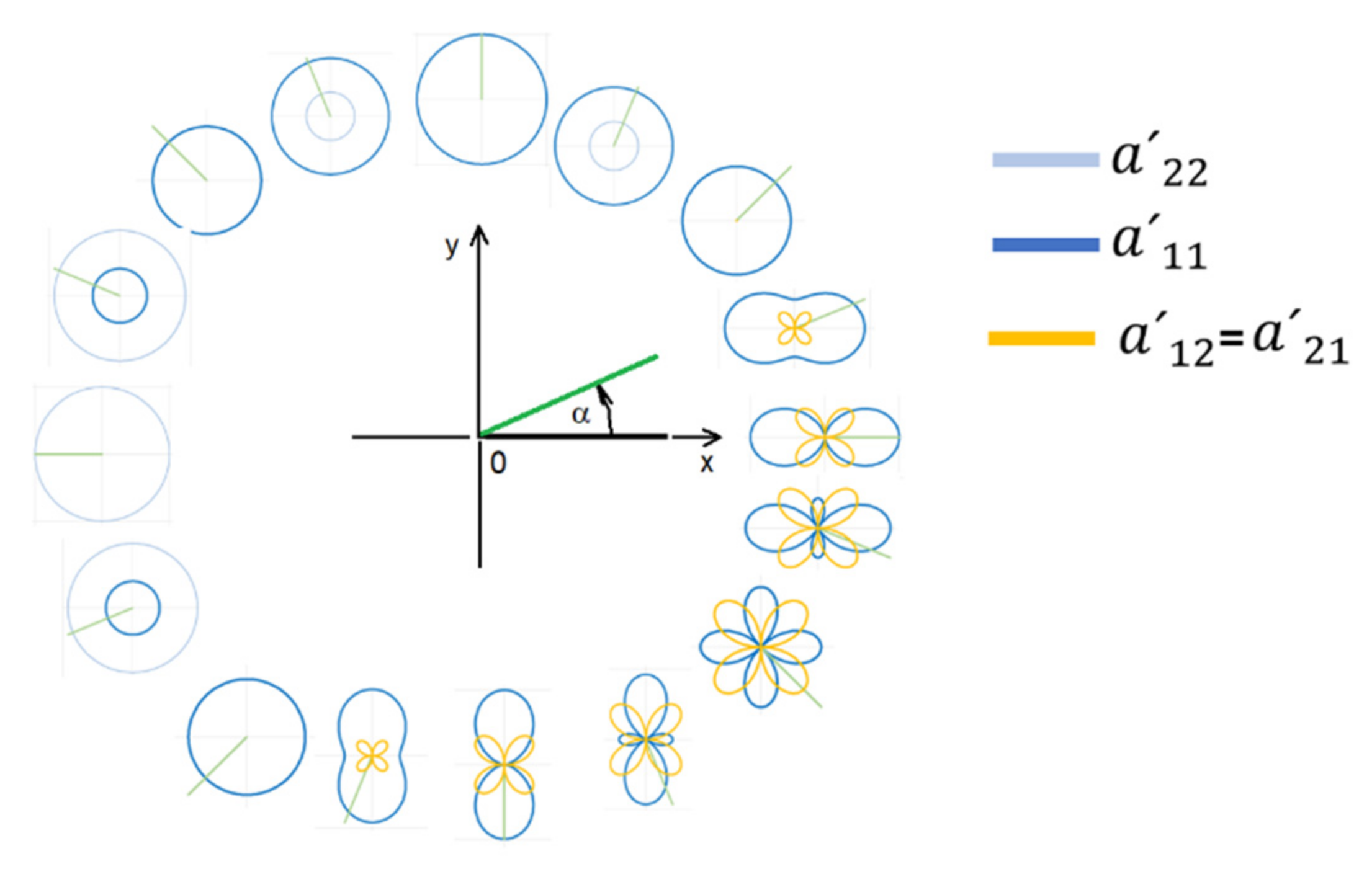
Visualization of tensor elements depending on angle means expressing the tensor elements through their decomposition into components of coordinate axes . Angle is determined immutably and is responsible for a particular tensor glyph form of the symmetric tensor in a plane. Individual coordinates are given by equations
Other components of tensors , , and are determined in a similar way.
The parameters are responsible for the tensor glyph form of a symmetric tensor rendered through visualization of elements of individual similar matrices depending on a change in angle . If a unit tensor norm is prescribed, then it is sufficient to characterize the tensor glyph form through a single parameter , where .
By changing the angle , all possible symmetric forms of tensor glyph are obtained as it is in the Figure 4. These forms are determined by a set of similar matrices. Under discrete division of angle , their number is finite. Since the individual adjacent forms are similar, the total number of possible forms is finite, too.
11. Discussion
The paper does not redact knowledge of tensor calculus, geometric algebra, and complex numbers theory available so far. In terms of calculations, all results are regular, and only the manner of interpretation of these known things is different, which enables a certain detached view of the issue of metric space. This new understanding of well-known things is facilitated by the use of new mathematical tools, summed up in the bullet points below:
- Lagrange’s identity and its relation to metric space;
- Enhancement of geometric product to include forms for which the result is a zero;
- Using the designation for wedge product of components, which resulted in the form of writing similar to that of the dot product of complex numbers;
- Use of two forms of the dot product of complex numbers;
- Introduction of total matrix and geometric product;
- Relativistic interpretation of a change in tensor values with respect to the base, resulting in writing the tensor in angular form and making it possible to obtain its visualization in the form of tensor glyph.
Basic spatial relations have been expressed for a 2D plane, as it is sufficiently simple and illustrative. It goes without saying that here, too, these means can be applied to higher dimensions.
12. Conclusions
A new view of known things through a new means of looking at them offers a certain clarification of some well-established definitions of mathematical entities, for example, definitions of divergence and curl. In this system, divergence and curl play the role of multivector components.
The value of this paper lies in a definition of the total matrix and geometric product in the form of a multivector, which features an added scalar part in addition to being written as a matrix. The link between the notation by indices of tensors and the angular writing of tensors using matrix eigenvalues is also pointed out. Overall, the main importance of the Lagrange’s identity is brought to the fore, as it is integrally related to vector space.
Author Contributions
Conceptualization, T.S.; methodology, T.S.; resources, T.S.; writing—original draft preparation, T.S.; supervision, M.L.; formal analysis, M.L.; writing—review and editing, J.S. and M.L.; project administration, J.S. All authors have read and agreed to the published version of the manuscript.
Funding
This work was supported by the Slovak Research and Development Agency under the Contract no. APVV-18-0413.
Acknowledgments
This work was supported by the Slovak Research and Development Agency under the Contract no. APVV-18-0413 and Contracts no. KEGA 016TUKE-4/2021, VEGA 1/0532/22.
Conflicts of Interest
The authors declare no conflict of interest. The founding sponsors had no role in the design of the study; in the collection, analyses, or interpretation of data; in the writing of the manuscript, and in the decision to publish the results.
References
- Lenoir, T. Descartes and the geometrization of thought: The methodological background of Descartes’ géométrie. Hist. Math. 1979, 6, 355–379. [Google Scholar] [CrossRef]
- Koecher, M. Lineare Algebra und Analytische Geometrie; Springer: Berlin/Heidelberg, Germany; New York, NY, USA, 2013; pp. 10–14. [Google Scholar]
- Hestenes, D.; Sobczyk, G.; Marsh, J. Clifford Algebra to Geometric Calculus. A Unified Language for Mathematics and Physics. Am. J. Phys. 1985, 53, 510–511. [Google Scholar] [CrossRef]
- Franchini, S.; Vassallo, G.; Sorbello, F. A brief introduction to Clifford algebra. Palermo (Italy) Univ. Degli Studi Di Palermo 2010, 24. [Google Scholar]
- Aragon-Camarasa, G.; Aragon-Gonzalez, G.; Aragon, J.L.; Rodriguez-Andrade, M.A. Clifford algebra with mathematica. arXiv 2008, arXiv:0810.2412. [Google Scholar]
- Hitzer, E. Introduction to Clifford’s geometric algebra. J. Soc. Instrum. Control Eng. 2012, 51, 338–350. [Google Scholar]
- Menti, A.; Zacharias, T.; Milias-Argitis, J. Geometric algebra: A powerful tool for representing power under nonsinusoidal conditions. IEEE Trans. Circuits Syst. I Regul. Pap. 2007, 54, 601–609. [Google Scholar]
- Hahn, A.J. The Clifford Algebra in the Theory of Algebras, Quadratic Forms, and Classical Groups. In Clifford Algebras; BirkhäuserL: Boston, UK, 2004; pp. 305–322. [Google Scholar]
- Knus, M.A. Quadratic Forms, Clifford Algebras and Spinors; ICEA: Zurich, Switzerland, 1988; pp. 40–48. [Google Scholar]
- Lasenby, A. Geometric algebra as a unifying language for physics and engineering and its use in the study of gravity. Adv. Appl. Clifford Algebras 2017, 27, 733–759. [Google Scholar] [CrossRef]
- Shirokov, D.S. Classification of Lie algebras of specific type in complexified Clifford algebras. Linear Multilinear Algebra 2018, 66, 1870–1887. [Google Scholar] [CrossRef]
- Sobczyk, G. Conformal mappings in geometric algebra. Not. AMS 2012, 59, 264–273. [Google Scholar]
- Montoya, F.G.; Baños, R.; Alcayde, A.; Arrabal-Campos, F.M.; Roldán-Pérez, J. Vector Geometric Algebra in Power Systems: An Updated Formulation of Apparent Power under Non-Sinusoidal Conditions. Mathematics 2021, 9, 1295. [Google Scholar] [CrossRef]
- Chappell, J.M.; Drake, S.P.; Seidel, C.L.; Gunn, L.J.; Iqbal, A.; Allison, A.; Abbott, D. Geometric algebra for electrical and electronic engineers. Proc. IEEE 2014, 102, 1340–1363. [Google Scholar] [CrossRef]
- Franchini, S.; Gentile, A.; Sorbello, F.; Vassallo, G.; Vitabile, S. Conformal ALU: A conformal geometric algebra coprocessor for medical image processing. IEEE Trans. Comput. 2014, 64, 955–970. [Google Scholar] [CrossRef]
- Hitzer, E.; Perwass, C. Interactive 3D space group visualization with CLUCalc and the Clifford geometric algebra description of space group. Adv. Appl. Clifford Algebras 2010, 20, 631–658. [Google Scholar] [CrossRef]
- Ricci, M.M.G.; Levi-Civita, T. Méthodes de calcul différentiel absolu et leurs applications. Math. Ann. 1900, 54, 125–201. [Google Scholar] [CrossRef]
- Sousa, C.D.; Cortesao, R. Inertia tensor properties in robot dynamics identification: A linear matrix inequality approach. IEEE/ASME Trans. Mechatron. 2019, 24, 406–411. [Google Scholar] [CrossRef]
- Rojas-Quintero, J.A.; Dubois, F.; Ramírez-de-Ávila, H.C. Riemannian Formulation of Pontryagin’s Maximum Principle for the Optimal Control of Robotic Manipulators. Mathematics 2022, 10, 1117. [Google Scholar] [CrossRef]
- Stylianou, F.; Pecnik, R.; Kassinos, S. A general framework for computing the turbulence structure tensors. Comput. Fluid 2015, 106, 54–66. [Google Scholar] [CrossRef]
- De Lathauwer, L.; De Moor, B.; Vandewalle, J. A multilinear singular value decomposition. SIAM J. Matrix Anal. Appl. 2000, 21, 1253–1278. [Google Scholar] [CrossRef]
- Carlini, E.; Catalisano, M.V.; Chiantini, L.; Geramita, A.V.; Woo, Y. Symmetric tensors: Rank, Strassen’s conjecture and e-computability. Ann. Della Sc. Norm. Super. Di Pisa Cl. Di Sci. 2018, 18, 1–28. [Google Scholar] [CrossRef]
- Blaga, A.M.; Nannicini, A. On Statistical and Semi-Weyl Manifolds Admitting Torsion. Mathematics 2022, 10, 990. [Google Scholar] [CrossRef]
- Borgo, R.; Kehrer, J.; Chung, D.H.; Maguire, E.; Laramee, R.S.; Hauser, H.; Ward, M.; Chen, M. Glyph-based visualization: Foundations, design guidelines, techniques and applications. In Eurographics State of the Art Reports; The Eurographics Association: Hannover, Germany, 2013; pp. 39–63. [Google Scholar]
- Gerrits, T.; Rössl, C.; Holger Theisel, H. Glyphs for general second-order 2d and 3d tensors. IEEE Trans. Vis. Comput. Graphics 2016, 23, 980–989. [Google Scholar] [CrossRef] [PubMed]
- Sarwar, T.; Ramamohanarao, K.; Zalesky, A. Mapping connectomes with diffusion MRI: Deterministic or probabilistic tractography? Magn. Reson. Med. 2019, 81, 1368–1384. [Google Scholar] [CrossRef] [PubMed]
- Muhammed, A.M.; Aswathi, V. Analysis of Visualization Techniques in Diffusion Tensor Imaging (DTI). In Proceedings of the 2018 Second International Conference on Advances in Electronics, Computers and Communications (ICAECC), Bengaluru, India, 9–10 February 2018. [Google Scholar]
- Brox, T.; Weickert, J.; Burgeth, B.; Mrázek, P. Nonlinear structure tensors. Image Vis. Comput. 2006, 24, 41–55. [Google Scholar] [CrossRef]
- Kratz, A.; Björn, M.; Hotz, I. A visual approach to analysis of stress tensor fields. In Scientific Visualization: Interactions, Features, Metaphors, 1st ed.; Hagen, H., Ed.; Schloss Dagstuhl—Leibniz-Zentrum für Informatik GmbH: Kaiserslautern, Germany, 2011; Volume 2, pp. 188–211. [Google Scholar]
- Kindlmann, G. Superquadric tensor glyphs. In Proceedings of the Sixth Joint Eurographics-IEEE TCVG Conference on Visualization, Konstanz, Germany, 19–24 May 2004; pp. 147–154. [Google Scholar]
- Schultz, T.; Kindlmann, G.L. Superquadric glyphs for symmetric second-order tensors. IEEE TVCG 2010, 16, 1595–1604. [Google Scholar] [CrossRef]
- Feragen, A.; Fuster, A. Geometries and Interpolations for Symmetric Positive Definite Matrices. Modeling, Analysis, and Visualization of Anisotropy; Springer: Cham, Switzerland, 2017; pp. 85–113. [Google Scholar]
- Stejskal, T.; Svetlík, J.; Dobránsky, J. An Analytical Method for Tensor Visualization in a Plane. Machines 2022, 10, 89. [Google Scholar] [CrossRef]
- Berberian, S.K. Linear Algebra; Oxford University Press: Oxford, MI, USA, 1992; pp. 286–287. [Google Scholar]
- Lim, L.H. Tensors in computations. Acta Numer. 2021, 30, 555–764. [Google Scholar] [CrossRef]
- Qi, Y.; Comon, P.; Lim, L.H. Uniqueness of nonnegative tensor approximations. IEEE Trans. Inf. Theory 2016, 62, 2170–2183. [Google Scholar] [CrossRef]
- Hestenes, D. Tutorial on geometric calculus. Adv. Appl. Clifford Algebras 2014, 24, 257–273. [Google Scholar] [CrossRef]
Figure 1.
Graphic representation of vectors of the geometric product and elements of the Lagrange’s identity.
Figure 1.
Graphic representation of vectors of the geometric product and elements of the Lagrange’s identity.

Figure 2.
Various forms of representing a point in plane: (a) real plane with a matrix vector product; (b) vector plane with a geometric vector product; (c) complex plane with a dot product of complex numbers.
Figure 2.
Various forms of representing a point in plane: (a) real plane with a matrix vector product; (b) vector plane with a geometric vector product; (c) complex plane with a dot product of complex numbers.

Figure 3.
Relationships transformability in a 2D plane.

Figure 4.
Change in the form of tensor glyph of a symmetric tensor depending on angle .

Publisher’s Note: MDPI stays neutral with regard to jurisdictional claims in published maps and institutional affiliations. |
© 2022 by the authors. Licensee MDPI, Basel, Switzerland. This article is an open access article distributed under the terms and conditions of the Creative Commons Attribution (CC BY) license (https://creativecommons.org/licenses/by/4.0/).
Share and Cite
MDPI and ACS Style
Stejskal, T.; Svetlík, J.; Lascsáková, M. Tensor of Order Two and Geometric Properties of 2D Metric Space. Mathematics 2022, 10, 3524. https://0-doi-org.brum.beds.ac.uk/10.3390/math10193524
AMA Style
Stejskal T, Svetlík J, Lascsáková M. Tensor of Order Two and Geometric Properties of 2D Metric Space. Mathematics. 2022; 10(19):3524. https://0-doi-org.brum.beds.ac.uk/10.3390/math10193524
Chicago/Turabian StyleStejskal, Tomáš, Jozef Svetlík, and Marcela Lascsáková. 2022. "Tensor of Order Two and Geometric Properties of 2D Metric Space" Mathematics 10, no. 19: 3524. https://0-doi-org.brum.beds.ac.uk/10.3390/math10193524
Note that from the first issue of 2016, this journal uses article numbers instead of page numbers. See further details here.