Analysis of a Queueing Model with MAP Arrivals and Heterogeneous Phase-Type Group Services

Abstract

Queueing models have proven to be very useful in real-life applications to enable the practitioners to optimize the limited resources to conduct their businesses as well as offer services efficiently. In general, we can group such applications into two sectors: manufacturing and service. These two sectors cover everything we deal with on a day-to-day basis. Queues in which the services are offered in blocks (or groups or batches) are well established in the literature and have a wide variety of applications in practice. In this paper, we look at one such queueing model in which the arrivals occur according to a Markovian arrival process and the services are offered in batches of varying sizes from 1 to a finite pre-determined constant, say, b. The service times are assumed to be of phase type with representation depending on the size of the group. Thus, the distributions considered are heterogeneous from both the representation and rate points of view. The model can be studied as a $GI/M/1$-type queue or as a $QBD$-model. The model is analyzed in steady state by establishing results including on the rate matrix and the waiting time distribution and providing a number of illustrative examples.

1. Introduction

It is well known that queueing models play a key role in many walks of life. Queues are part and parcel of everything we do daily. These queues can be physical or virtual. Virtual queues are more prevalent these days due to permeation of the Internet and e-commerce into our daily activities. Various industries and businesses such as manufacturing, airlines, package delivery, pharmaceutical, hospitals, restaurants, Internet, and supply chain, among others, use queueing models to optimize their functions so as to efficiently serve the customers/clients. In general, we can group such applications into manufacturing and service sectors. These two sectors cover everything we deal with on a day-to-day basis. For example, the cell phone which has integrated into our activities has manufacturing (using needed raw materials to make it) and service (repairing and maintaining when needed) aspects; when visiting a grocery store to pick up items for our daily consumption of food, we notice that these items have all gone through some type of a “production“ process involving manufacturing as well as service. Similarly, one can identify the components of each and every item we consume or replace or replenish on a regular basis.

The study of the classical queueing models depends on the (a) type of arrival process (renewal or correlated); (b) service times (general or specific ones such as phase-type distribution); (c) service scheme (first-come-first-served, service in random order, priority, etc); (d) number of servers; and (e) buffer capacity (finite or infinite), among others.

Queueing models in which the customers are served in batches (of size of 1 or more), which is also referred to as general bulk service rule (see [1]), have been studied in the literature for more than five decades. While to do an exhaustive literature survey on such models will itself constitute a separate (review) paper, which is probably overdue and worthwhile, here we will mention a few references that contain a number of key references to bulk queues. It should be pointed out that some of these references deal with variations to the classical queueing models such as server vacations, server working vacations, inventory (needed for offering services), and retrials, among others [1,2,3,4,5,6,7,8,9]. Note that these references include a lot of other references, and for the sake of the length of the paper, we did not include them and refer the reader to the quoted ones here.

As mentioned in [2,3], very few papers have focused on correlated arrival processes with batch services such that the service times are non-exponential. Recently, a few authors (see, [2,3,4,7,8]) studied batch service queueing models in which the arrivals occur according to a Markovian arrival process, and the services are offered in batches of varying sizes. The service times in [3,4,7,8] for a batch of size, say, r, is modeled using the maximum of r identical $PH-$distributions, which again is of $PH-$type (see [10,11,12,13]). Normally, one uses the maximum (which is an order statistic) of r distributions to model the services in the context of a multi-server system so that the system can assign as many servers as the number in a batch, and the service of the batch is over at the time when the last customer’s service is completed. Such models have been studied in the context of cloud/grid computing (see, e.g., [14]).

The model studied in [2] deals with a finite capacity queue, and the bulk services are generally distributed. Furthermore, the service times depend on the size of the group, and the authors use an embedded Markov renewal process approach to study the model in steady state. The illustrative numerical examples presented assume phase-type services with the rates depending on the number served in a batch.

In [3], the authors consider a $MAP/PH/1$ queueing model in which the services are offered in batches of a fixed size, say, b. At a service completion, if the number of customers waiting in the queue is at least b, the server offers a service by taking exactly b customers. However, if the number waiting is less than b, a clock (referred to as an admission clock) is started, whose lifetime is modeled using a $PH$-distribution. If before the expiration of this clock, the number in the queue hits b, the clock is turned off, and a service begins with b customers. If the clock expires before the bth customer arrives, then the server takes all those customers waiting and offers a service. Thus, in this way, a service for a group of size varying between 1 and $b-1$ is offered. If the number of customers waiting in the queue is 0, a new admission period is started. Recall that in [2], the service times are of phase type and are obtained as the maximum of a finite number (which is the size of the group that is offered a service) of identical phase-type distribution.

The model studied in this paper differs from the above two papers as follows.

• Compared to [2], here, we look at an infinite capacity system, and the study is based on using the $QBD$ process. Furthermore, we use Neuts’ caudal characteristic curve analysis to bring out the qualitative nature of the model under study. Such a study has not been fully explored in the literature. While the approach presented in [2] is applicable to services having varying dimensions for the underlying $PH-$distributions, the numerical examples presented there are for the case where only the rates are varied.
• Compared to [3], here, the server offers services as long as there is at least one customer waiting in the queue. Thus, upon the completion of a service, if the queue is non-empty, the server will offer services to the minimum of the number in the queue and b. Otherwise, the server will remain idle until a new arrival occurs. Note that if the rate of the admission period is increased to infinity (i.e, the admission period instantaneously expires, leading the server to offer services to the waiting customers as long as the queue is non-empty), their model should lead to the model studied here. However, it is not clear from the presentation in [3] how their results including the rate matrix, R, in the limiting case look like. As pointed out above, we use Neuts’ caudal characteristic curve analysis to bring out the qualitative nature of the model under study. Thus, our paper can be viewed as a companion to [3] as well as the limiting case (as the admission rate approaches infinity).

The paper is organized as follows. In Section 2, we present the model studied in this paper, and the steady-state analysis of the model, including some key results, are discussed in Section 3. Illustrative numerical examples to bring out the qualitative nature of the model are discussed in Section 4, and finally, in Section 5, we present a summary and future work on this model.

We use the following notations which are consistent with the ones set forth in the literature. The dimensions of the vectors and the matrices will be of appropriate size as dictated in the context where these are used. When further clarifications are needed, we will denote the dimension in the context.

• e is a column vector of 1s.
• “T” appearing in the superscript stands for transpose. Thus, ${\mathit{e}}^{\mathit{T}}$ is a row vector of 1 s.
• ${\mathit{e}}_i$ is a column vector with 1 in the ith position and 0 elsewhere.
• I is an identity matrix.
• $\mathrm{\Delta }\left(\mathit{a}\right)$ is a diagonal matrix whose diagonal elements are given by the entries of the vector a.
• ⊗ and ⊕, respectively, are the Kronecker product and Kronecker sum.

2. Description of the Model

We consider a single server queue in which arrivals occur according to an $MAP$ with an irreducible representation $(D_0,D_1)$ of dimension m, where $D_0$ governs transitions corresponding to no arrivals and $D_1$ governs those that result in arrivals. Let $\mathbf{\delta }$ denote the invariant vector of the generator $D=D_0+D_1$. That is, $\mathbf{\delta }$ satisfies

$$\mathbf{\delta }D=\mathbf{0}\mathrm{and}\mathbf{\delta }\mathit{e}=1.$$

(1)

The arrival rate, $\lambda$, is thus given by $\lambda =\mathbf{\delta }{D}_1\mathit{e}$. The Markovian arrival process has been introduced by Neuts in a more general setup as a versatile Markovian arrival process in the 1970s, and since then, these processes have found enormous applications in practice. For details on $MAP$ and associated processes, we refer the reader to [10,11,12,15,16,17,18,19,20,21,22].

There is a single server who offers services in batches of varying sizes from 1 to b, where b is a pre-determined finite positive integer. Upon completion of a service, the server will become idle if there is no customer waiting in the queue. Otherwise, the server will offer services to the waiting customers by picking the minimum of b and the number waiting from the head of the queue. Thus, the services can be for b or less depending on the size of the queue. The service times are assumed to be of phase type ($PH$) whose representation depends on r, the number served in the group, and is given by $({\mathbf{\beta }}_r,S_r)$ of order $n_r$, for $1\le r\le b$. Let ${\mu }_r={\left[{\mathbf{\beta }}_r{(-S_r)}^{-1}\mathit{e}\right]}^{-1},1\le r\le b$, denote the service rate when the server is serving a batch of r customers. $PH$-distributions were introduced by Neuts [23], and their simple matrix formalism makes it much more efficient to use in stochastic modeling, which has been amply demonstrated in the queueing literature. For more details on $PH$-distributions and their properties, we refer the reader to [10,11,12,13]. For later use, we define

$${\mathbf{\zeta }}_r={\mu }_r{\mathbf{\beta }}_r{(-S_r)}^{-1},1\le r\le b.$$

(2)

note that ${\mathbf{\zeta }}_r$ is the invariant vector of the irreducible generator $S_r+{\mathit{S}}_{\mathit{r}}^{\mathbf{0}}{\mathit{\beta }}_r,$ where ${\mathit{S}}_{\mathit{r}}^{\mathbf{0}}$ is such that $S_r\mathit{e}+{\mathit{S}}_{\mathit{r}}^{\mathbf{0}}=\mathbf{0},1\le r\le b$. While there needs to be no restriction on the service rates for the analysis to be carried out later, we do assume (for practical reasons) that ${\mu }_1\ge {\mu }_2\ge \cdots \ge {\mu }_b$. The rationale for this restriction, as it helps to devise illustrative numerical examples, is as follows. When serving more than one customer, it is natural that the service time may be longer on average as compared to serving only one customer. Furthermore, the time to serve a batch of customers should not be the sum of the individual service times of the customers in the batch. In [3,8], the authors assume, for the sake of generating numerical examples, that the service time of a batch of r customers is obtained as the maximum of r identical $PH$-distributions, which again is of phase type (see, e.g., [10,11,12,13]). Obviously, the means of the $PH$-distributions will increase as r is increased. Or equivalently, the rates of the services will decrease as r is increased.

Upon completion of a service, the server will (a) become idle due to an empty queue or (b) serve a batch of $min\{b,N_q\}$ customers, where $N_q$ is the number in the queue at that moment.

The system described above can be studied as a Markov process as follows. Suppose that we define

• $N\left(t\right)$ = number of customers in the queue at time t.
• $M_1\left(t\right)$ = phase of the service, if any, at time t.
• $M_2\left(t\right)$ = phase of the arrival process at time t.
• $\mathrm{\Omega }=\{(0,k):1\le k\le m\}\bigcup \{(i,j_r,k):1\le j_r\le n_r,1\le r\le b,1\le k\le m,i\ge 0\}$.
• $\mathbf{\ast }=\left\{\right(0,k):1\le k\le m\}$.
• $\mathbf{(}\mathit{i}\mathbf{,}\mathit{j}\mathbf{)}=\{(i,r,k):1\le r\le n_j,1\le k\le m\}$, for $1\le j\le b,i\ge 0$.
• $\mathit{i}=\{\mathbf{(}\mathit{i}\mathbf{,}\mathbf{1}\mathbf{)},\mathbf{(}\mathit{i}\mathbf{,}\mathbf{2}\mathbf{)},\cdots ,\mathbf{(}\mathit{i}\mathbf{,}\mathit{b}\mathbf{)}\}$, for $i\ge 0$.
• $n=n_1+\cdots +n_b$.

The three-dimensional process $\{(N\left(t\right),M_1\left(t\right),M_2\left(t\right)):t\ge 0\}$ is a Markov process on the state space $\mathrm{\Omega }$ as defined above. Note that level ∗ consisting of m states corresponds to the system (or the server) being in idle state; the level $\mathbf{(}\mathit{i}\mathbf{,}\mathit{j}\mathbf{)}$, consisting of $m{n}_j,1\le j\le b,$ states, corresponds to the case where there are i customers in the queue and the server is busy serving a batch of j customers. Finally, the level mathvariant="bold", for $i\ge 0$, consisting of $mn$ states, corresponds to the case where the system has i customers in the queue and that the server is busy serving a batch of customers. The batch size could be anywhere from 1 to b. The generator of the Markov process is given by

$$Q=\begin{array}{c}\mathbf{*}\\ \mathbf{0}\\ \mathbf{1}\\ \mathbf{2}\\ \mathbf{⋮}\\ \mathbf{b}\\ \mathbf{b}\mathbf{+}\mathbf{1}\\ \mathbf{b}\mathbf{+}\mathbf{2}\\ \mathbf{⋮}\end{array}\left(\begin{array}{ccccccccccc}*& \mathbf{0}\hfill & \mathbf{1}& \mathbf{2}& \mathbf{3}& \cdots & \mathbf{b}& \mathbf{b}+\mathbf{1}& \mathbf{b}+\mathbf{2}& \mathbf{b}+\mathbf{3}& \cdots \\ D_0& \hfill ({\beta }_1\otimes D_1,\mathbf{0})\hfill & 0& 0& 0& \cdots & 0& 0& 0& 0& \cdots \\ C_0& A_1\hfill & A_0& 0& 0& \cdots & 0& 0& 0& 0& \cdots \\ 0& C_1\hfill & A_1& A_0& 0& \cdots & 0& 0& 0& 0& \cdots \\ 0& C_2\hfill & 0& A_1& A_0& \cdots & 0& 0& 0& 0& \cdots \\ ⋮& ⋮\hfill & ⋮& ⋮& ⋮& \cdots & ⋮& ⋮& ⋮& \cdots \\ 0& C_b\hfill & 0& 0& 0& \cdots & A_1& A_0& 0& 0& \cdots \\ 0& 0\hfill & A_2& 0& 0& \cdots & 0& A_1& A_0& 0& \cdots \\ 0& 0\hfill & 0& A_2& 0& \cdots & 0& 0& A_1& A_0& \cdots \\ ⋮& ⋮\hfill & ⋮& ⋮& ⋮& ⋮& ⋮& ⋮& ⋮& \cdots \end{array}\right)$$

(3)

, where

$$C_0=\left(\begin{array}{c}{\mathit{S}}_1^0\otimes I\\ {\mathit{S}}_2^0\otimes I\\ ⋮\\ {\mathit{S}}_b^0\otimes I\end{array}\right),C_j=\left(\begin{array}{ccccccc}0& \cdots & 0& {\mathit{S}}_1^0{\mathbf{\beta }}_j\otimes I& 0& \cdots & 0\\ \\ 0& \cdots & 0& {\mathit{S}}_2^0{\mathbf{\beta }}_j\otimes I& 0& \cdots & 0\\ ⋮& \cdots & ⋮& ⋮& ⋮& \cdots & ⋮\\ 0& \cdots & 0& {\mathit{S}}_b^0{\mathbf{\beta }}_j\otimes I& 0& \cdots & 0\end{array}\right),1\le j\le b,$$

(4)

$$A_0=I_n\otimes D_1,A_1=\mathrm{\Delta }(S_1\oplus D_0,S_2\oplus D_0,\cdots ,S_b\oplus D_0),A_2=C_b.$$

(5)

it is worth pointing out the interpretation of the entries of Q. An idle system (namely, system in level ∗) will enter into level 0 through an arrival. At that instant, a new service for a batch of size 1 will begin. This transition is governed by the entry $({\mathbf{\beta }}_1\otimes D_1,\mathbf{0}).$ When the system is in level 0 and should there be a transition out of this level, it has to be to either level ∗ through a service completion or to level 1 through an arrival. These are, respectively, governed by the entries $C_0$ and $A_0$. The entry $A_1$ governs the transitions within level 0. Due to the services being offered in groups of size not exceeding b, it is clear that when the system is in level $\mathit{r},1\le r\le b,$ the possible transitions out of level r are either to level 0 or to level $\mathit{r}\mathbf{+}\mathbf{1}$ and these are, respectively, governed by $C_r$ and $A_0$. The transitions within level r are governed by $A_1$.

Note that the generator Q given in Equation (3) is of $GI/M/1$-type queue, and one can apply the results for such a paradigm developed by Neuts (see, e.g., [10,13,24]). However, by combining the levels in a certain way, we can the study the model under consideration as a $QBD$-process. As mentioned in [24], there are advantages and disadvantages as the size of the problem increases going from a $GI/M/1$-type to $QBD$-process. However, the sparsity of the coefficient matrices enables one to exploit the structure, as we will demonstrate below.

3. Analysis of the Model in Steady State

In this section, we perform the steady-state analysis of the model under study. Toward this end, we first establish the stability condition.

Theorem 1.

The model under study is stable if and only if the condition

$$\lambda <b{\mu }_b.$$

(6)

Proof. 

Suppose we denote the level $\tilde{\mathit{i}}=\{\mathit{b}\mathbf{(}\mathit{i}\mathbf{-}\mathbf{1}\mathbf{)}\mathbf{+}\mathrm{1},\cdots ,\mathit{b}\mathit{i}\}$, for $i\ge 1$. Then, the generator, say, $\tilde{Q}$ of the Markov process of the model under study is of the form

$$\tilde{Q}=\left(\begin{array}{ccccccc}{D}_0& ({\mathbf{\beta }}_1\otimes D_1,\mathbf{0})& 0& 0& 0& 0& \cdots \\ C_0& A_1& {\mathit{e}}_1^T\otimes A_0& 0& 0& 0& \cdots \\ 0& \tilde{C}& {\tilde{A}}_1& {\tilde{A}}_0& 0& 0& \cdots \\ 0& 0& {\tilde{A}}_2& {\tilde{A}}_1& {\tilde{A}}_0& 0& \cdots \\ 0& 0& 0& {\tilde{A}}_2& {\tilde{A}}_1& {\tilde{A}}_0& \cdots \\ ⋮& ⋮& ⋮& \ddots & \ddots & \ddots & \cdots \end{array}\right)$$

(7)

where

$$\begin{array}{c}\tilde{C}=\left(\begin{array}{c}{C}_1\\ C_2\\ ⋮\\ C_b\end{array}\right),{\tilde{A}}_0=\left(\begin{array}{cccc}0& 0& \cdots & 0\\ 0& 0& \cdots & 0\\ ⋮& ⋮& \cdots & ⋮\\ 0& 0& \cdots & 0\\ A_0& 0& \cdots & 0\end{array}\right),{\tilde{A}}_1=\left(\begin{array}{cccccc}{A}_1& A_0& 0& 0& \cdots & 0\\ 0& A_1& A_0& 0& \cdots & 0\\ 0& 0& A_1& A_0& \cdots & 0\\ ⋮& ⋮& ⋮& \ddots & \cdots & ⋮\\ 0& 0& 0& 0& \cdots & A_1\end{array}\right),\\ \hfill {\tilde{A}}_2=I_b\otimes A_2.\hfill \end{array}$$

(8)

□

We now have a $QBD$ process for the model under study and can apply the known tools (see, e.g., [10,13,24]). We will briefly outline the steps including the ones for exploiting the structure of the coefficient matrices.

Let $\tilde{\mathbf{\pi }}$ be the invariant vector of the generator $\tilde{A}={\tilde{A}}_0+{\tilde{A}}_1+{\tilde{A}}_2$ so that we have $\tilde{\mathbf{\pi }}\tilde{A}=\mathbf{0}$ and $\tilde{\mathbf{\pi }}\mathit{e}=1.$ Noting that

$$\tilde{A}=\left(\begin{array}{ccccccc}{A}_1+A_2& A_0& 0& 0& \cdots & 0& 0\\ 0& A_1+A_2& A_0& 0& \cdots & 0& 0\\ 0& 0& A_1+A_2& A_0& \cdots & 0& 0\\ ⋮& ⋮& ⋮& ⋮& \cdots & ⋮& ⋮\\ 0& 0& 0& 0& \cdots & A_1+A_2& A_0\\ A_0& 0& 0& 0& \cdots & 0& A_1+A_2\end{array}\right)$$

(9)

is cyclic, the vector $\tilde{\mathbf{\pi }}$ is of the form

$$\tilde{\mathbf{\pi }}=\frac{1}{b}({\mathit{e}}^{\mathit{T}}\otimes \mathbf{\pi }),$$

(10)

with $\mathbf{\pi }$ being the invariant vector of the generator $A=A_0+A_1+A_2$. Since

$$A=\left(\begin{array}{ccccccc}{S}_1\oplus D& 0& 0& 0& \cdots & 0& {\mathit{S}}_{\mathbf{1}}^{\mathbf{0}}{\mathbf{\beta }}_{\mathit{b}}\otimes I\\ 0& S_2\oplus D& 0& 0& \cdots & 0& {\mathit{S}}_{\mathbf{2}}^{\mathbf{0}}{\mathbf{\beta }}_{\mathit{b}}\otimes I\\ ⋮& ⋮& ⋮& ⋮& \cdots & ⋮& ⋮\\ 0& 0& 0& 0& \cdots & 0& (S_b+{\mathit{S}}_{\mathit{b}}^{\mathbf{0}}{\mathbf{\beta }}_{\mathit{b}})\oplus D\end{array}\right),$$

(11)

is reducible, it is clear that we have

$$\mathbf{\pi }=(\mathbf{0},\mathbf{0},\cdots ,\mathbf{0},{\mu }_b{\mathbf{\beta }}_b{(-S_b)}^{-1}\otimes \mathbf{\delta }).$$

(12)

Using the fact that the model under study is a $QBD$-process, the stability condition is given by (see, e.g., [13,24])

$$\tilde{\mathbf{\pi }}{\tilde{A}}_0\mathit{e}<\tilde{\mathbf{\pi }}{\tilde{A}}_2\mathit{e}.$$

(13)

For our model, the condition given in Equation (13) with the help of Equations (10) and (12) immediately yields $\frac{\lambda }{b}<{\mu }_b$ and hence the stated result.

The rate matrix, denoted by $\tilde{R}$, plays an important role in matrix–analytic methods (see, e.g., [10,12,13,21,24,25]). We briefly discuss the structure of this rate matrix. Here, the rate matrix satisfies the following matrix–quadratic equation

$${\tilde{R}}^2{\tilde{A}}_2+\tilde{R}{\tilde{A}}_1+{\tilde{A}}_0=0,$$

(14)

and the following theorem establishes the structure of $\tilde{R}$.

Theorem 2.

The rate matrix, $\tilde{R}$, of dimension $n{b}^2$ is of the form

$$\tilde{R}=\left(\begin{array}{ccccc}0& 0& 0& \cdots & 0\\ 0& 0& 0& \cdots & 0\\ ⋮& ⋮& ⋮& \cdots & ⋮\\ R& R^2& R^3& \cdots & R^b\end{array}\right),$$

(15)

where the matrix R of dimension $nb$ is given by

$$R=\left(\begin{array}{cccccc}{R}_1& 0& 0& \cdots & 0& {\widehat{R}}_1\\ 0& R_2& 0& \cdots & 0& {\widehat{R}}_2\\ ⋮& ⋮& ⋮& \cdots & ⋮& ⋮\\ 0& 0& 0& \cdots & R_{b-1}& {\widehat{R}}_{b-1}\\ 0& 0& 0& \cdots & 0& R_b\end{array}\right).$$

(16)

The elements of R are obtained as follows. The matrices $R_j,1\le j\le b-1$, of dimension $n_{j}m$ are explicitly computed as

$$R_j=(I\otimes D_1)[-{(S_j\oplus D_0)}^{-1}],1\le j\le b-1,$$

(17)

and $R_b$ is the minimal non-negative solution to

$$R_b^{b+1}({\mathit{S}}_{\mathit{b}}^{\mathbf{0}}{\mathbf{\beta }}_{\mathit{b}}\otimes I)+R_b(S_b\oplus D_0)+(I\otimes D_1)=0.$$

(18)

The rest of the (block) elements of R are obtained in terms of the other (block) matrices as

$$R_j^{b+1}({\mathit{S}}_{\mathit{j}}^{\mathbf{0}}{\mathbf{\beta }}_{\mathbf{b}}\otimes I)+\sum _{k=0}^b{R}_j^{b-k}{\widehat{R}}_j{R}_b^k(S_b\oplus D_0)=0,1\le j\le b-1.$$

(19)

Proof. 

The fact that $\tilde{R}$ has only the last (block) row entries to be nonzero follows immediately on noting that (a) $\tilde{R}{\tilde{A}}_2\mathit{e}={\tilde{A}}_0\mathit{e}$, (b) ${\tilde{A}}_0\mathit{e}$ has the only nonzero block entry occurring in the last row; and (c) $\tilde{R}$ is non-negative. The probabilistic interpretation of the rate matrix in continuous-time (this is the approach we have taken here), in general, (see, e.g., [10,13,25]) states that for states away from the boundary, the $(j,k)$th entry of the rate matrix gives the average time (calculated in terms of the units of the sojourn time in state $(i,j)$) spent in state $(i+1,k)$ before reaching level i, given that we started in state $(i,j)$. In our context, due to the three-dimensional process as well as grouping b states as $\tilde{\mathit{i}}=\{\mathit{b}(\mathit{i}-\mathbf{1})+\mathbf{1},\cdots ,\mathit{b}\mathit{i}\}$ to obtain the $QBD$ process, this probabilistic interpretation together with the structure of the coefficient matrices yields the structure of the last (block) row of $\tilde{R}$ as given in Equation (15). There is a similar probabilistic interpretation for the states within level $\tilde{i}$; on noting the structure again and for the levels away from the boundary, it is clear that we have the structure for R as given in Equation (16). The key here is that away from the boundary, the server upon completing a service will always offer services to a group of b customers. The stated Equations (17) through (19) follow immediately by expanding Equation (14) with the help of the structures given in Equations (15) and (16). □

Remark 1.(1) The equations given in Equation (19) have explicit solutions. To see this, suppose that we denote $\tau \left(B\right)$ to be the direct (row) sum of the matrix B. Recall that $\tau \left(B\right)$ is obtained by stringing the rows of B into one long row vector. Thus, if B is an $p\times q$ matrix, then $\tau \left(B\right)$ is a row vector of dimension $pq$ obtained by stringing the rows of B into one row. Using the properties of the direct sum (see, e.g., [10] for a summary of these), we can write Equation (19) as, for $1\le j\le b-1$,

$$\tau \left({\widehat{R}}_j\right)=\tau \left(R_j^{b+1}\right)(I\otimes {\mathit{S}}_{\mathit{j}}^{\mathbf{0}}{\mathbf{\beta }}_{\mathit{b}}\otimes I){\left(-\sum _{k=1}^b\left[{\left(R_j^{b-k}\right)}^T\otimes R_b^k({\mathit{S}}_{\mathit{j}}^{\mathbf{0}}{\mathbf{\beta }}_{\mathit{b}}\otimes I)\right]-I\otimes (S_b\oplus D_0)\right)}^{-1}.$$

(20)

(2) The coefficient matrices appearing in Equations (17) through (20) are so sparse that one can exploit them, especially when the dimensions are large. For example, to compute $R_j,1\le j\le b$, we proceed as follows. Let $B=\left\{B_{rk}\right\}=-{(S_j\oplus D_0)}^{-1}$. Note that $B_{rk},1\le r,k\le b$, are of dimension m. Denoting by $S_j^{\left(rk\right)}$ the $(r,k)$th element of $S_j$, it is easy to verify the following system of equations

$$B_{rk}=\left[{\delta }_{rk}I+\sum _{t=1,t\ne k}^{n_j}{B}_{rt}{S}_j^{\left(tk\right)}\right]{(-S_j^{\left(kk\right)}I-D_0)}^{-1},1\le r,k\le n_j,$$

(21)

where ${\delta }_{rk}$ is the Kronecker delta taking values of 0 or 1 depending on whether $r=k$ or $r\ne k$. Since the right-hand side of the above equation has matrices that are all non-negative, the equations are numerically stable. Once B is computed, the $(r,k)$th element of $R_j$ is calculated as $D_1{B}_{rk}$. Similarly, the other matrices are computed by exploiting the special structure produced by Kronecker products and sums.

We are now ready to discuss the steady-state probability vector of the generator Q. Let $\mathit{x}=({\mathit{x}}^{*},{\mathit{x}}_0,{\mathit{x}}_1,\cdots )$ denote the steady-state vector of Q such that

$$\mathit{x}Q=\mathbf{0}\mathrm{a}\mathrm{n}\mathrm{d}\mathit{x}\mathit{e}=1.$$

(22)

Note the following interpretations of the components of x.

• ${\mathit{x}}^{*}$, of dimension m, gives the steady-state probability vector that the system is idle with the arrival process in one of the m phases.
• ${\mathit{x}}_i$, of dimension $mn$, gives the steady-state probability vector that the system has exactly i customers in the queue and the server and the arrival process are in various phases.

Defining ${\tilde{\mathit{x}}}_i=({\mathit{x}}_{b(i-1)+1},\cdots ,{\mathit{x}}_{bi}),i\ge 1,$ we see that Equation (22) is equivalent to

$$({\mathit{x}}^{*},{\mathit{x}}_0,{\tilde{\mathit{x}}}_1,{\tilde{\mathit{x}}}_2,\cdots )\tilde{Q}=0\mathrm{and}({\mathit{x}}^{*},{\mathit{x}}_0,{\tilde{\mathit{x}}}_1,{\tilde{\mathit{x}}}_2,\cdots )\mathit{e}=1.$$

(23)

We now state the result on the steady-state vector.

Theorem 3.

The steady-state vector $\tilde{\mathit{x}}$ is obtained by solving the following equations

$$\begin{array}{c}{\mathit{x}}^{*}{D}_0+{\mathit{x}}_0{C}_0=\mathbf{0},\\ \\ {\mathit{x}}^{*}({\mathbf{\beta }}_1\otimes D_1,\mathbf{0})+{\mathit{x}}_0{A}_1+{\displaystyle \sum _{k=1}^b}{\mathit{x}}_k{C}_k=\mathbf{0},\\ \\ {\mathit{x}}_{j-1}{A}_0+{\mathit{x}}_j{A}_1+{\mathit{x}}_b{R}^j{A}_2=\mathbf{0},1\le j\le b,\\ \\ {\mathit{x}}_i={\mathit{x}}_b{R}^{i-b},i\ge b,\\ \\ {\mathit{x}}^{*}\mathit{e}+{\displaystyle \sum _{i=0}^{\infty }}{\mathit{x}}_i\mathit{e}=1.\end{array}$$

(24)

Proof. 

Starting at the macro level, we see that the steady-state vector x is written as

$$\begin{array}{c}{\mathit{x}}^{*}{D}_0+{\mathit{x}}_0{C}_0=\mathbf{0},\\ \\ {\mathit{x}}^{*}({\mathbf{\beta }}_1\otimes D_1,\mathbf{0})+{\mathit{x}}_0{A}_1+{\tilde{\mathit{x}}}_1\tilde{C}=\mathbf{0},\\ \\ {\mathit{x}}_0({\mathit{e}}_1^T\otimes A_0)+{\tilde{\mathit{x}}}_1[{\tilde{A}}_1+\tilde{R}{\tilde{A}}_2]=\mathbf{0},\\ \\ {\tilde{\mathit{x}}}_i={\tilde{\mathit{x}}}_1{\tilde{R}}^{i-1},i\ge 1,\\ \\ {\mathit{x}}^{*}\mathit{e}+{\mathit{x}}_0\mathit{e}+{\tilde{\mathit{x}}}_1{(I-\tilde{R})}^{-1}\mathit{e}=1.\end{array}$$

(25)

Due to the structures of $\tilde{R}$ (see Equation (14)) and R (see Equation (16)), the above equations can further be simplified to yield the stated result. □

Remark 2.(1) Note that the vectors ${\mathit{x}}_i,i\ge b+1,$ as given in Equation (24), are explicitly known from the knowledge of ${\mathit{x}}_b$ and R. Thus, obtaining the steady-state vector $\tilde{\mathit{x}}$ reduces to solving the first three equations given in (24) along with the normalizing equation given by ${\mathit{x}}^{*}\mathit{e}+{\displaystyle \sum _{j=0}^{b-1}}{\mathit{x}}_j\mathit{e}+{\mathit{x}}_b{(I-R)}^{-1}\mathit{e}=1.$

(2) The steady-state equations can be solved using one of several methods such as the (block) Gauss–Seidel method by exploiting the structure of the coefficient matrices. For example, one can exploit the structure of the coefficient matrices appearing in Equation (24). For example, the first equation given there is simplified as

$${\mathit{x}}^{*}=\sum _{k=1}^b\sum _{r=1}^{n_k}{\mathit{x}}_{0kr}{S}_{kr}^0{(-D_0)}^{-1},$$

where ${\mathit{x}}_0$ is partitioned into vectors of dimension m as

$${\mathit{x}}_0=({\mathit{x}}_{011},\cdots ,{\mathit{x}}_{01n_1},\cdots ,{\mathit{x}}_{0b1},\cdots ,{\mathit{x}}_{0b{n}_b})$$

and $S_{kr}^0$ is the rth component of the vector ${\mathit{S}}_k^0$.

Stationary Waiting Time in the Queue

We now focus on the stationary waiting time (in the queue) distribution of an arriving customer. Toward this end, we first define the steady-state vector at arrivals to be $\mathit{z}=(z^{*},{\mathit{z}}_1,{\mathit{z}}_2,\cdots )$ such that $z^{*}$ gives the probability that an arriving customer finds the system empty and hence the waiting time in the queue will be zero, and ${\mathit{z}}_i$, of dimension n, gives the steady-state probability vector that an arriving customer will see the system busy with i in the queue (including the arrived one) and the server is busy with 1 or more (but up to b) in service and the phase of the current service in various states. Note that to find the waiting time distribution in the queue, one does not need to keep track of the arrival phase. However, one needs to keep track of the phase of the arrival process for deriving an expression for the waiting time in the system. This is due to the fact that the service time depends on the batch size, and if the arrived customer is not the bth customer in a batch, then there is a possibility that the future arrivals might make a difference in the service of time of the batch that has the arrived customer. It is easy to verify that

$$z^{*}=\frac{1}{\lambda }{\mathit{x}}^{*}{D}_1\mathit{e}\mathrm{and}{\mathit{z}}_i=\frac{1}{\lambda }{\mathit{x}}_{i-1}(I\otimes D_1\mathit{e}),i\ge 1.$$

(26)

The following theorem gives an expression for the Laplace transform of the stationary waiting time in the queue of an arrival.

Theorem 4.

The Laplace transform ($LT$), $w_q^{*}\left(s\right)$, of the stationary waiting time in the queue of an arrival is given by

$$w_q^{*}\left(s\right)=z^{*}+\sum _{i=1}^{\infty }{\widehat{\mathit{z}}}_i{\left[{(sI-S)}^{-1}F\right]}^{i-1}{(sI-S)}^{-1}{\mathit{S}}^{\mathbf{0}},R\mathit{e}\left(s\right)\ge 0,$$

(27)

where

$${\widehat{\mathit{z}}}_i=\sum _{k=b(i-1)+1}^{bi}{\mathit{z}}_k,i\ge 1.$$

(28)

$$\begin{array}{c}F=\left(\begin{array}{cccc}0& 0& \cdots & {\mathit{S}}_{\mathbf{1}}^{\mathbf{0}}{\mathbf{\beta }}_{\mathit{b}}\\ 0& 0& \cdots & {\mathit{S}}_{\mathbf{2}}^{\mathbf{0}}{\mathbf{\beta }}_{\mathit{b}}\\ ⋮& ⋮& \cdots & ⋮\\ 0& 0& \cdots & {\mathit{S}}_{\mathit{b}}^{\mathbf{0}}{\mathbf{\beta }}_{\mathit{b}}\end{array}\right),S=\mathrm{\Delta }(S_1,S_2,\cdots ,S_b),{\mathit{S}}^{\mathbf{0}}=\left(\begin{array}{c}{\mathit{S}}_{\mathbf{1}}^{\mathbf{0}}\\ {\mathit{S}}_{\mathbf{2}}^{\mathbf{0}}\\ ⋮\\ {\mathit{S}}_{\mathit{b}}^{\mathbf{0}}\end{array}\right).\end{array}$$

(29)

Proof. 

First, observe that for the waiting time in the queue, we do not need to keep track of the phase of the arrival process once the tagged customer enters into the system. Secondly, an arriving customer finding the system idle will enter service immediately, and so, the waiting time in the queue is zero. This occurs with probability $z^{*}$ and hence justifies the first term of the $LT$. Suppose now that the tagged customer finds the server busy with $i-1$ customers waiting in the queue. At this instant, the number waiting (including the tagged customer) is i. If $i\le b$, the waiting time of the tagged customer is the remaining service time of the current one. Basically, the number of service completions needed before the tagged customer enters service depends on how many batches of size b are formed. The actual position within the batch of the tagged customer does not matter. These observations enable us to see that the waiting time in the queue can be modeled as the time until absorption in a continuous-time Markov chain with the generator given by

$$Q_{W_q}=\left(\begin{array}{ccccccc}0& \mathbf{0}& \mathbf{0}& \mathbf{0}& \mathbf{0}& \mathbf{0}& \cdots \\ \mathit{e}\otimes S^0& I\otimes S& 0& 0& 0& 0& \cdots \\ \mathbf{0}& I\otimes F& I\otimes S& 0& 0& 0& \cdots \\ \mathbf{0}& 0& I\otimes F& I\otimes S& 0& 0& \cdots \\ \mathbf{0}& 0& 0& I\otimes F& I\otimes S& 0& \cdots \\ ⋮& ⋮& ⋮& ⋮& ⋮& ⋮& \cdots \end{array}\right.$$

(30)

The stated result follows immediately on noting that (a) the continuous-time Markov chain with generator $Q_{W_q}$ given in Equation (30) has the initial probability vector $(z^{*},{\mathit{z}}_1,{\mathit{z}}_2,\cdots )$. This is based on (a) what an arriving customer will see as the state of the system at that epoch and the fact that (b) ${(-S)}^{-1}F\mathit{e}=\mathit{e}$ and $F{(-S)}^{-1}\mathit{e}={\mu }_b^{\prime }{\mathit{S}}^{\mathbf{0}}.$ □

Corollary 1.

The mean waiting time in the queue is given by

$$\begin{array}{c}{\mu }_{W_q}^{\prime }=-\frac{d{w}^{*}\left(s\right)}{ds}{]}_{s=0}=\frac{1}{\lambda }{\displaystyle \sum _{k=0}^{b-1}}{\displaystyle \sum _{j=1}^b}{\mathit{x}}_{kj}\left({(-S_j)}^{-1}\mathit{e}\otimes D_1\mathit{e}\right)\\ \\ +\frac{{\mu }_b^{\prime }}{\lambda }{\mathit{x}}_b{(I-R)}^{-1}\left[{(I-R^b)}^{-1}+I\right](\mathit{e}\otimes D_1\mathit{e}).\end{array}$$

(31)

4. Illustrative Numerical Examples

In this section, we present a few illustrative examples to point out the qualitative behavior of the model under study. For this, we need to define a number of system performance measures. These are as follows.

• System Performance Measures: Here, we list a few key system performance measures along with their formulas.

1.

P (system or server is idle) = ${\mathit{x}}^{*}\mathit{e}$.

2.

P (server is busy) = 1 − ${\mathit{x}}^{*}\mathit{e}$.

3.

Given that the server is busy, the conditional $PMF$, $\left\{{\xi }_j\right\}$, of the number in service is

$${\xi }_j=\frac{1}{1-{\mathit{x}}^{*}\mathit{e}}\left[\sum _{i=0}^{b-1}{\mathit{x}}_i+{\mathit{x}}_b{(I-R)}^{-1}\right]({\mathit{e}}_j\otimes \mathit{e}),1\le j\le b.$$

with the knowledge of $\left\{{\xi }_j\right\}$, we can compute the (conditional) mean, ${\mu }_{NiS}$, number in service and other measures.

4.

The mean number of customers in the queue is calculated as

$${\mu }_{N_q}=\sum _{i=1}^{b-1}i{\mathit{x}}_i\mathit{e}+{\mathit{x}}_b{(I-R)}^{-2}\mathit{e}+(b-1){\mathit{x}}_b{(I-R)}^{-1}\mathit{e}.$$

5.

The spectral radius, say $\eta$, of the rate matrix R plays an important role in matrix–analytic methods. Neuts [26] introduced the term caudal characteristic curve obtained by plotting $\eta$ against the traffic intensity $\rho =\frac{\lambda }{b\mu }$. This is applicable to all models that possess the matrix–geometric solution. Basically, this curve tells the behavior of the queue length with regard to its upsurges (i.e., queues staying in longer duration whenever they become longer). Because of this behavior, one cannot use the mean queue length as a reliable measure in comparing various models. We refer the reader to [26] as well as [24] for more details on this.

6.

Using probabilistic interpretation, the mean recurrence time to an empty system (i.e., the mean of the times between the system reaching an idle state) is given by ${\mu }_{RT}^{\prime }={\left[{\mathit{x}}_{0}F\mathit{e}\right]}^{-1}={\left[{\mathit{x}}^{*}{D}_1\mathit{e}\right]}^{-1}$.

7.

With the knowledge of the mean recurrence time, we can obtain the mean idle time as ${\mu }_I^{\prime }={\mathbf{\mu }}_{RT}^{\prime }{\mathit{x}}^{*}\mathit{e}$ and the mean busy period as ${\mu }_{BP}^{\prime }={\mu }_{RT}^{\prime }-{\mu }_I^{\prime }$.

• Accuracy checks: One of the key aspects in numerical computation is to make sure the results have internal accuracy checks. Toward this end, we list the following accuracy checks. For use in the sequel, we define $\mathit{a}=({\mathit{a}}_1,{\mathit{a}}_2,\cdots ,{\mathit{a}}_{\mathit{b}})$ as

  $$\mathit{a}=\sum _{i=0}^{b-1}{\mathit{x}}_i+{\mathit{x}}_b{(I-R)}^{-1}.$$

  Note that ${\mathit{a}}_j$, of dimension $m{n}_j$, gives the probability vector that the server is busy serving j customers with the arrival process and the service in various phases.

• Accuracy check 1: One of the properties of the rate matrix in the $QBD$ model is $\tilde{R}{\tilde{A}}_2\mathit{e}={\tilde{A}}_0\mathit{e}$. In our model under study, due to the structure of $\tilde{R}$ (see Equation (14)), this reduces to

  $${(I-R)}^{-1}R(I-R^b)({\mathit{S}}^{\mathbf{0}}\otimes \mathit{e})=(\mathit{e}\otimes D_1\mathit{e}).$$

  The above equation can be rewritten in terms of smaller dimensions by exploiting the structure of the R matrix as given in Equation (16). The details are similar to the exploitation mentioned earlier and hence omitted.

• Accuracy check 2: This one is intuitively clear, as in steady state, the phase of the arrival process should be equal to the one obtained directly (see Equation (1)). That is,

  $${\mathit{x}}^{\mathbf{*}}+\mathit{a}(\mathit{e}\otimes I)=\mathbf{\delta }.$$
• Accuracy check 3: This one is intuitively clear, as in steady state, the joint phases of the arrival process and the service should be equal to the one obtained directly (see Equations (1) and (2)). That is,

  $$\frac{1}{{\theta }_j}\mathit{a}({\mathit{e}}_j\otimes I)=({\mathbf{\zeta }}_j\otimes \mathbf{\delta }),1\le j\le b,$$

  where ${\theta }_j$ is the probability that the server is busy with a batch of j customers and is given by

  $${\theta }_j={\mathit{a}}_j\mathit{e},1\le j\le b.$$
• Accuracy check 4: This one is intuitively clear, as in steady state, the average rate of arrivals should be equal to the average rate of departures. That is,

  $$\sum _{j=1}^{b}j{\mathit{a}}_j({\mathit{S}}_{\mathit{j}}^{\mathbf{0}}\otimes \mathit{e})=\lambda .$$

  for our illustrative examples, we look at five different $MAPs$ covering renewal and correlated arrivals. We use the following notation for ease of display. $ERL(k,\tau )$ denotes an Erlang distribution of order k with rate $\tau$ in each of the k phases. $HE(\mathit{p},\mathbf{\vartheta })$ denotes an hyperexponential distribution with parameter vector $\mathbf{\vartheta }=({\vartheta }_1,\cdots ,{\vartheta }_k)$ with mixing probability vector $\mathit{p}=(p_1,\cdots ,p_k)$. That is, we have an hyperexponential distribution involving k exponentials with parameters ${\vartheta }_r$ with corresponding probability $p_r$, for $1\le r\le k$.

The five $MAPs$ for the arrival processes include three renewal processes, one negatively correlated process and one positively correlated process. Note that for the renewal process, we use special cases of phase-type distribution, and the corresponding representation in terms of $MAP$ parameters is clear (see, [10]). Thus, if we use a $PH$-distribution with representation, say $(\mathbf{\alpha },L)$ of order m, then the corresponding $MAP$ representation is given by $D_0=L$ and $D_1={\mathit{L}}^{\mathbf{0}}\mathbf{\alpha }$, where ${\mathit{L}}^{\mathbf{0}}=-L\mathit{e}$.

• ERA: This is $ERL(5,5)$.
• EXA: This is $ERL(1,1)$, that is, we have a Poisson process with parameter 1.
• HEA: This is $HE(p,\mathbf{\vartheta })$ with

  $$\mathit{p}=(0.5,0.3,0.15,0.04,0.01)\mathrm{and}\mathbf{\vartheta }=(2.18,1.09,0.545,0.2725,0.13625).$$

  The two correlated, negative and positive, processes are as follows:
• NCA: This is negatively correlated $MAP$ with representation matrices given by

  $$\begin{array}{c}{D}_0=\left(\begin{array}{ccccc}-2.25& 2.25& 0& 0& 0\\ 0& -2.25& 2.25& 0& 0\\ 0& 0& -2.25& 2.25& 0\\ 0& 0& 0& -2.25& 0\\ 0& 0& 0& 0& -4.5\end{array}\right),D_1=\left(\begin{array}{ccccc}0& 0& 0& 0& 0\\ 0& 0& 0& 0& 0\\ 0& 0& 0& 0& 0\\ 0.0225& 0& 0& 0& 2.2275\\ 4.455& 0& 0& 0& 0.045\end{array}\right).\end{array}$$
• PCA: This is negatively correlated $MAP$ with representation matrices given by

  $$\begin{array}{c}{D}_0=\left(\begin{array}{ccccc}-2.25& 2.25& 0& 0& 0\\ 0& -2.25& 2.25& 0& 0\\ 0& 0& -2.25& 2.25& 0\\ 0& 0& 0& -2.25& 0\\ 0& 0& 0& 0& -4.5\end{array}\right),D_1=\left(\begin{array}{ccccc}0& 0& 0& 0& 0\\ 0& 0& 0& 0& 0\\ 0& 0& 0& 0& 0\\ 2.2275& 0& 0& 0& 0.0225\\ 0.045& 0& 0& 0& 4.455\end{array}\right).\end{array}$$

  All the above five $MAPs$ have an arrival rate of 1. The standard deviations of the inter-arrival times are, respectively, 0.44721, 1, 1.69710, 1.01227, and 1.01227. The 1-lag correlation coefficient of the successive inter-arrival times are, respectively, 0, 0, 0, −0.57855, and 0.57855.

For services, we look at the following $PH$-distributions. Since we discuss examples with $b=5$, only sets of five distributions are needed.

• $E{R}_1:$ This is $ERL(5,5{\mu }_1)$.
• $E{R}_2:$ This is $ERL(4,4{\mu }_2)$.
• $E{R}_3:$ This is $ERL(3,3{\mu }_3)$.
• $E{R}_4:$ This is $ERL(2,2{\mu }_4)$.
• $E{R}_5:$ This is $ERL(1,{\mu }_5)$.
• $H{E}_1:$ This is $HE(\mathit{p},\mathbf{\vartheta })$ with $\mathit{p}=(0.6,0.2,0.15,0.04,0.01)\mathrm{and}\mathbf{\vartheta }={\mu }_5(10,5,3,2,1).$
• $H{E}_2:$ This is $HE(\mathit{p},\mathbf{\vartheta })$ with $\mathit{p}=(0.7,0.15,0.10,0.05)\mathrm{and}\mathbf{\vartheta }={\mu }_4(10,5,2,1).$
• $H{E}_3:$ This is $HE(\mathit{p},\mathbf{\vartheta })$ with $\mathit{p}=(0.8,0.15,0.05)\mathrm{and}\mathbf{\vartheta }={\mu }_3(10,5,1).$
• $H{E}_4:$ This is $HE(\mathit{p},\mathbf{\vartheta })$ with $\mathit{p}=(0.9,0.1)\mathrm{and}\mathbf{\vartheta }={\mu }_4(10,1).$
• $H{E}_5:$ This is exponential with parameter ${\mu }_5$. That is, $HE(p,\vartheta )$ with $p=1\mathrm{and}\vartheta ={\mu }_5.$

The parameter ${\mu }_1$ will be chosen so that for a given $\rho$, ${\mu }_1=\frac{\lambda }{\rho }$. The other parameters here are chosen as ${\mu }_r=\frac{{\mu }_1}{r},2\le r\le 5$. This guarantees that $\rho =\frac{\lambda }{5{\mu }_5}$ and also satisfies the property ${\mu }_1\ge {\mu }_2\ge {\mu }_3\ge {\mu }_4\ge {\mu }_5$.

Example 1.

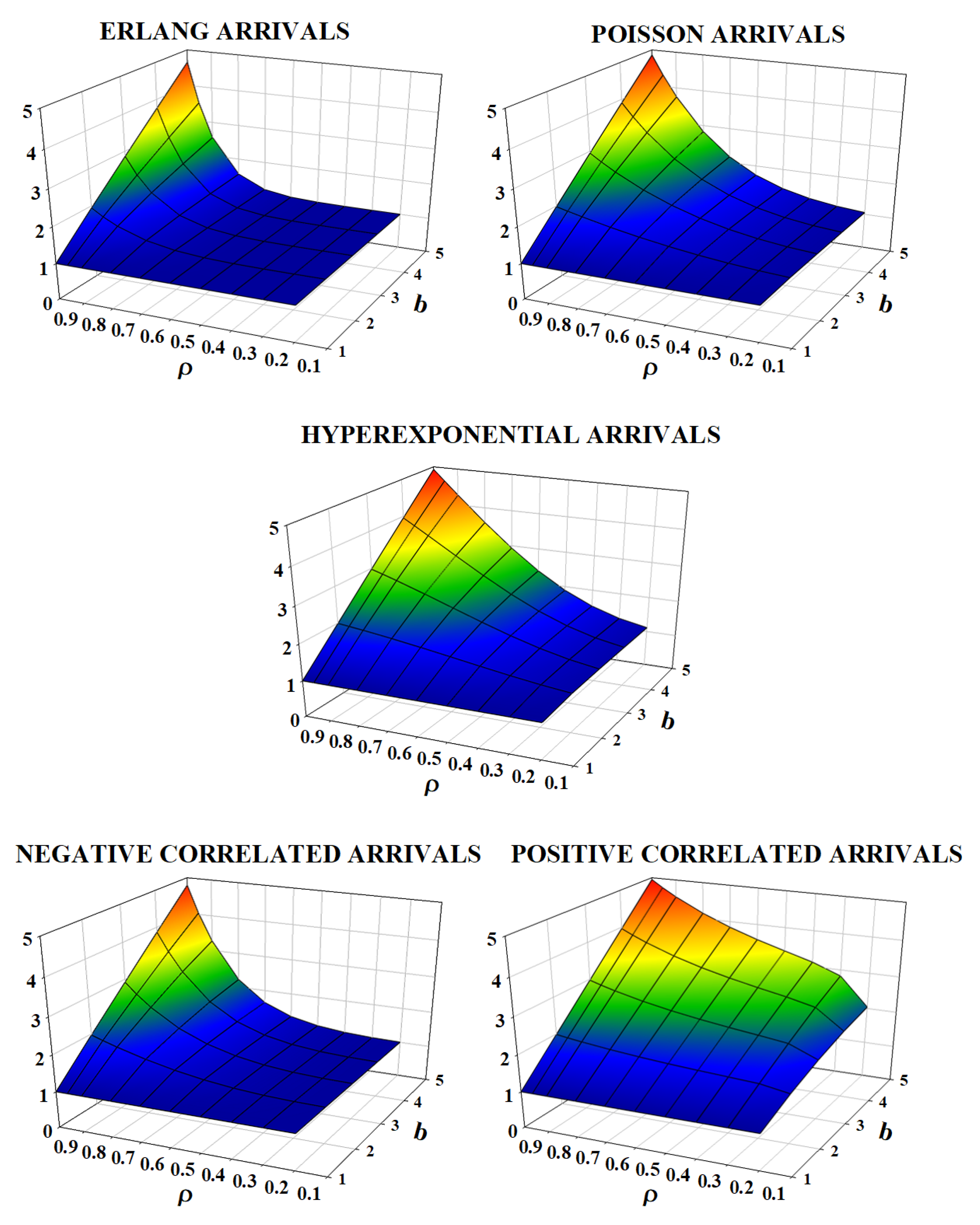
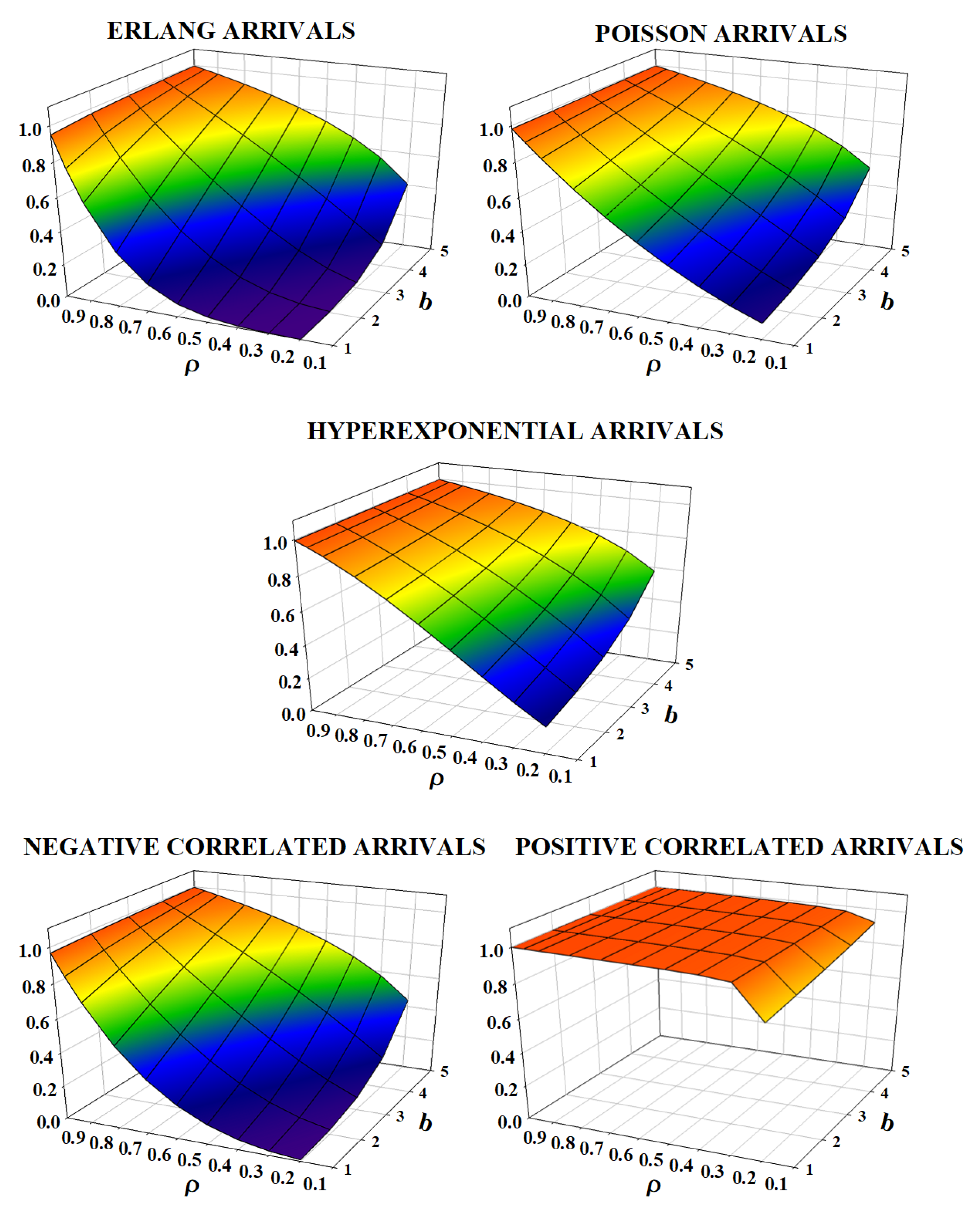
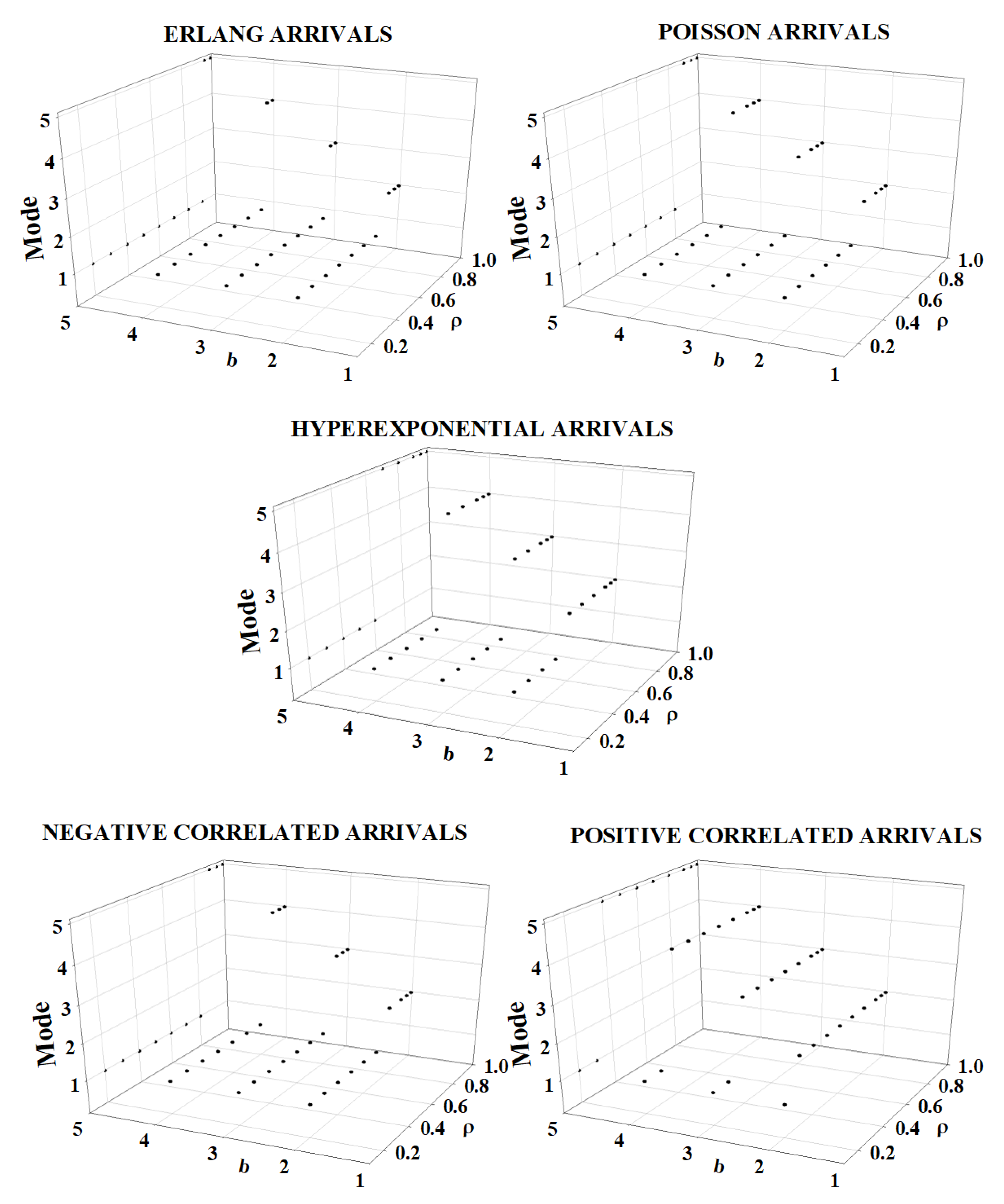
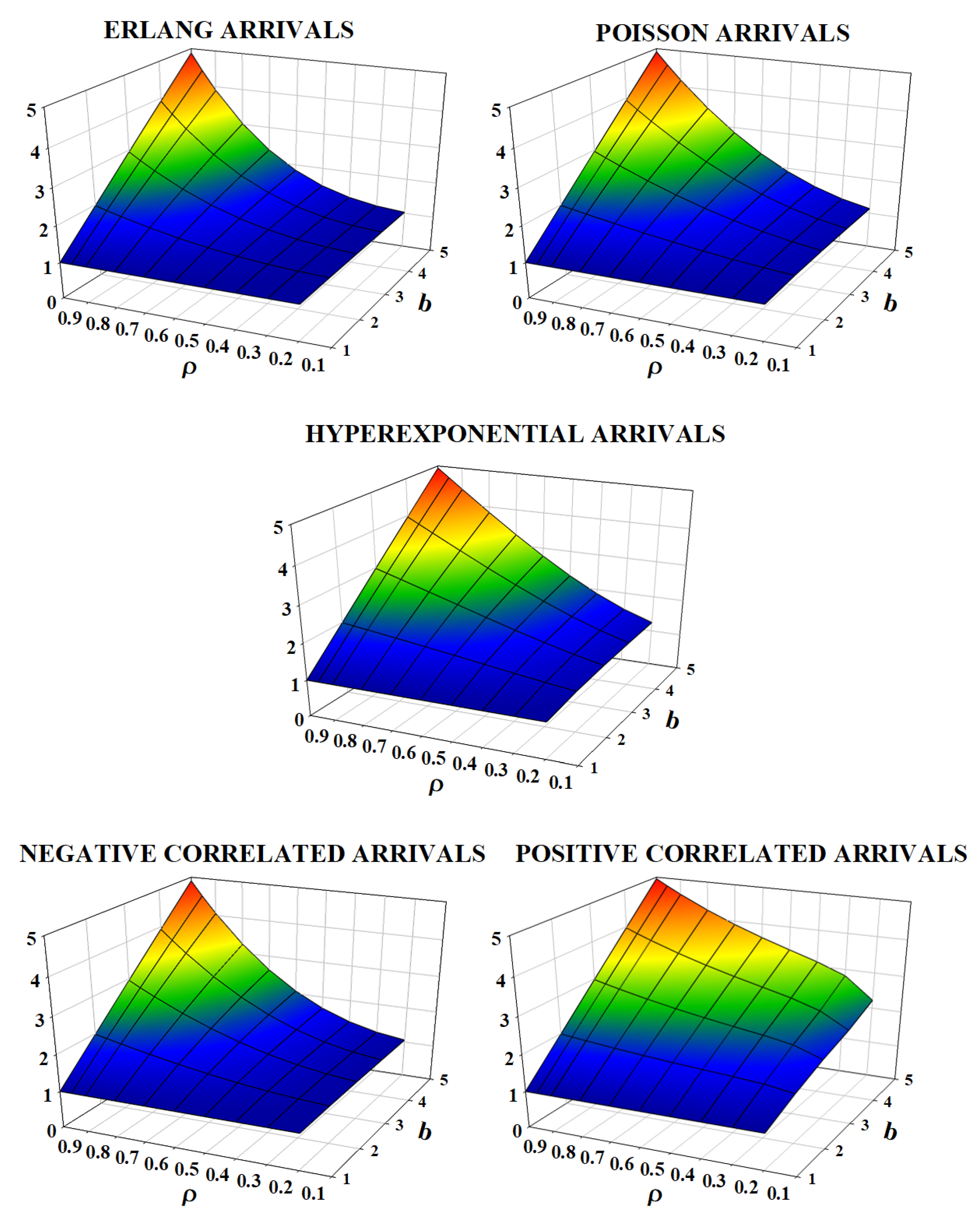
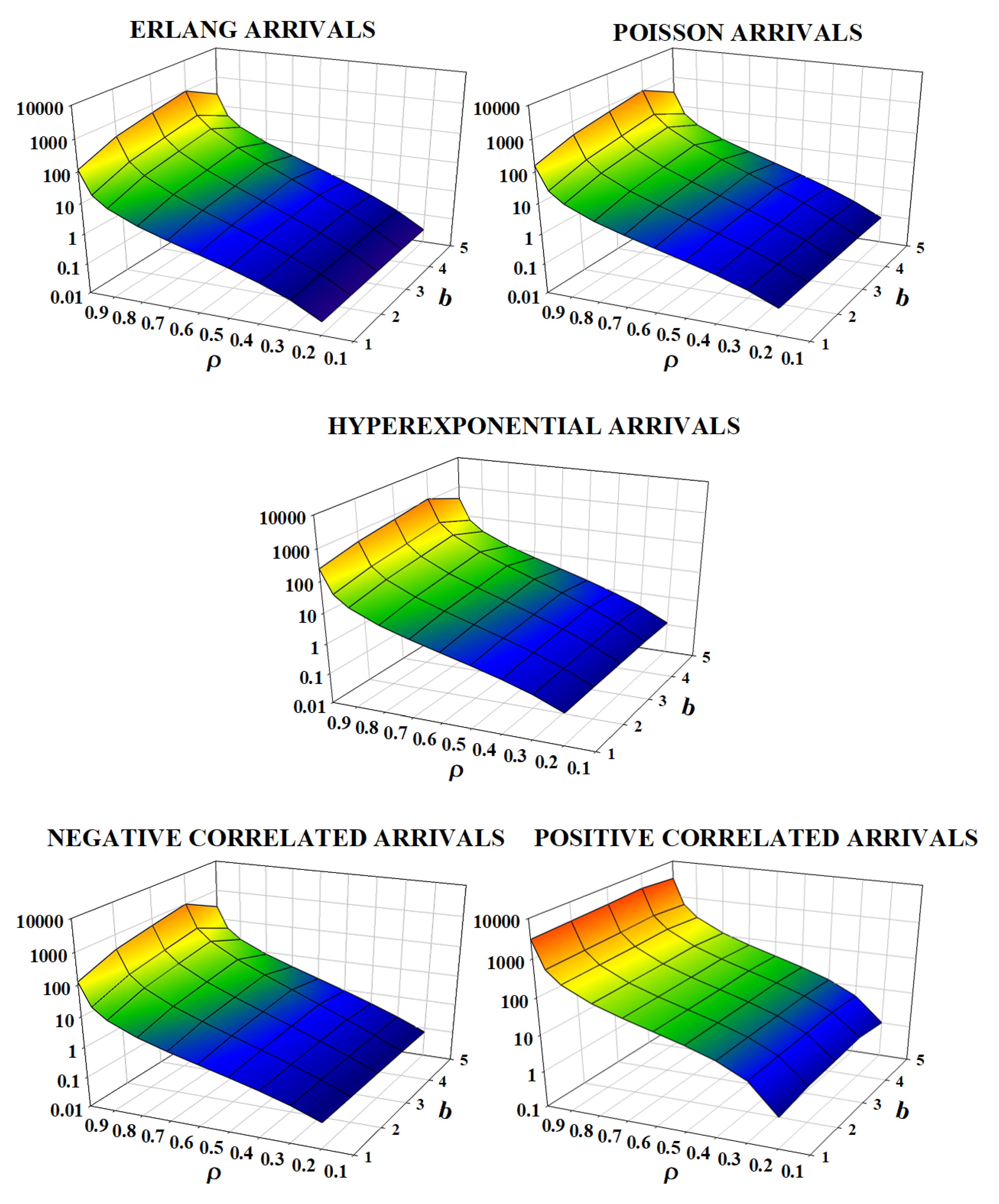
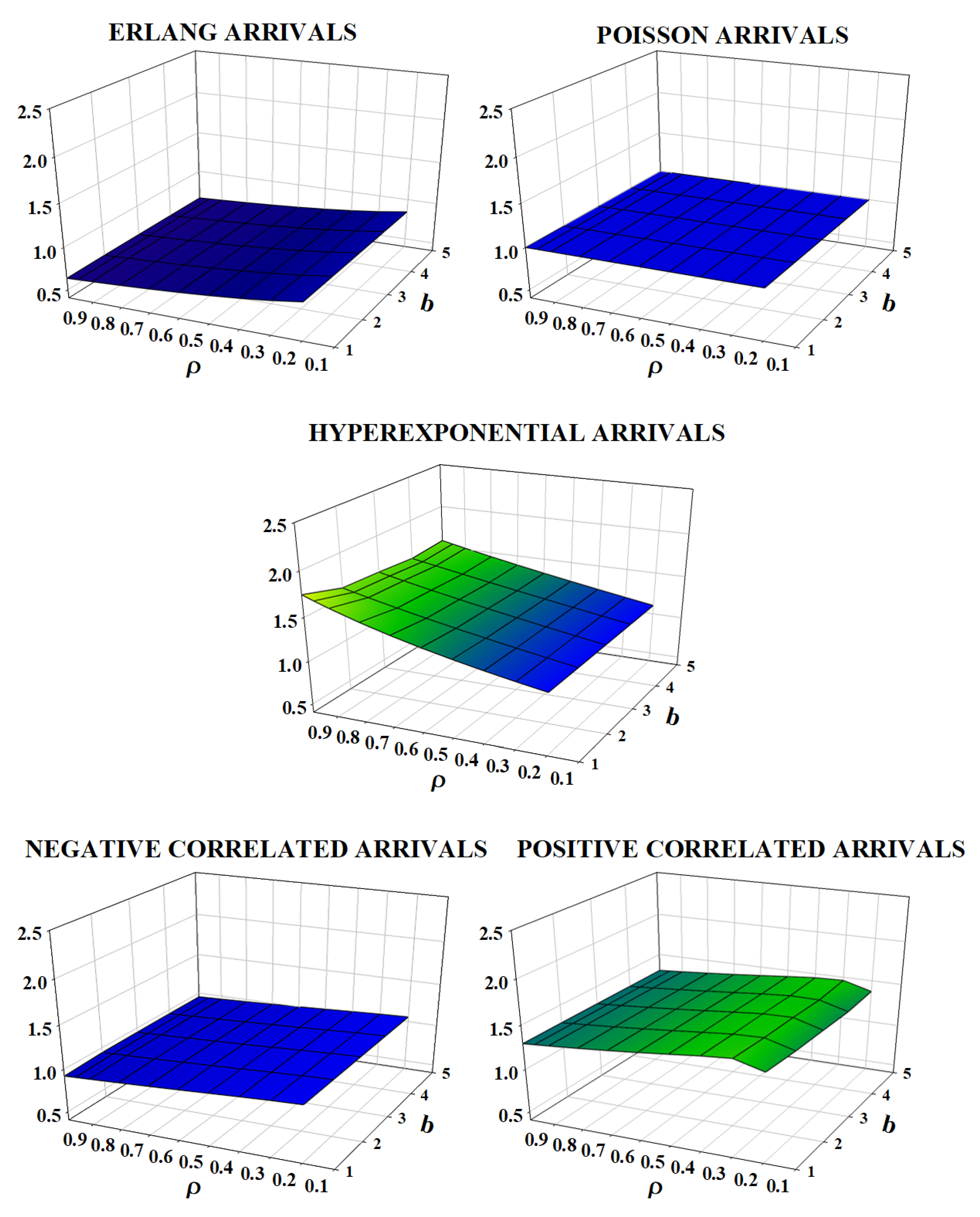
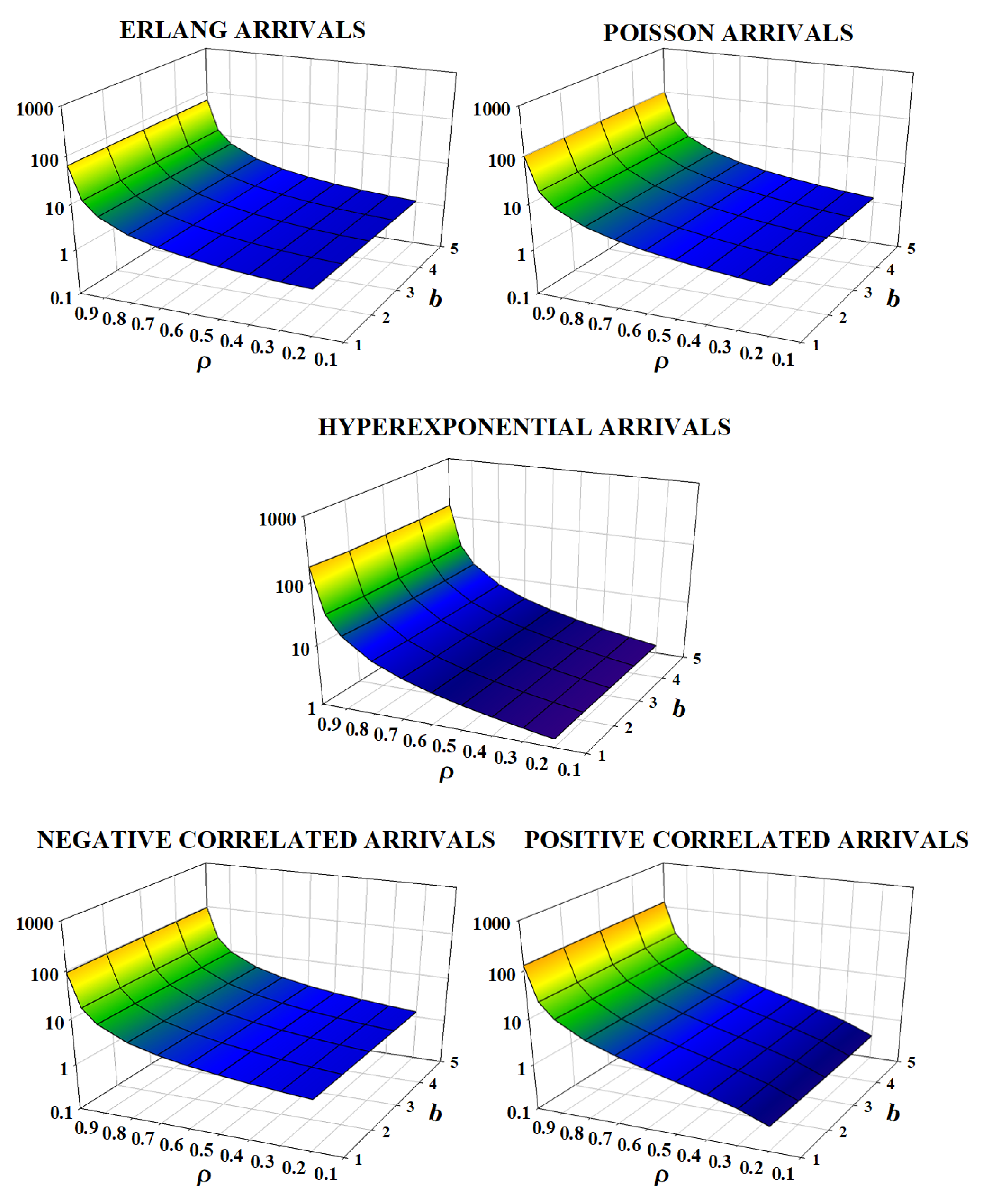
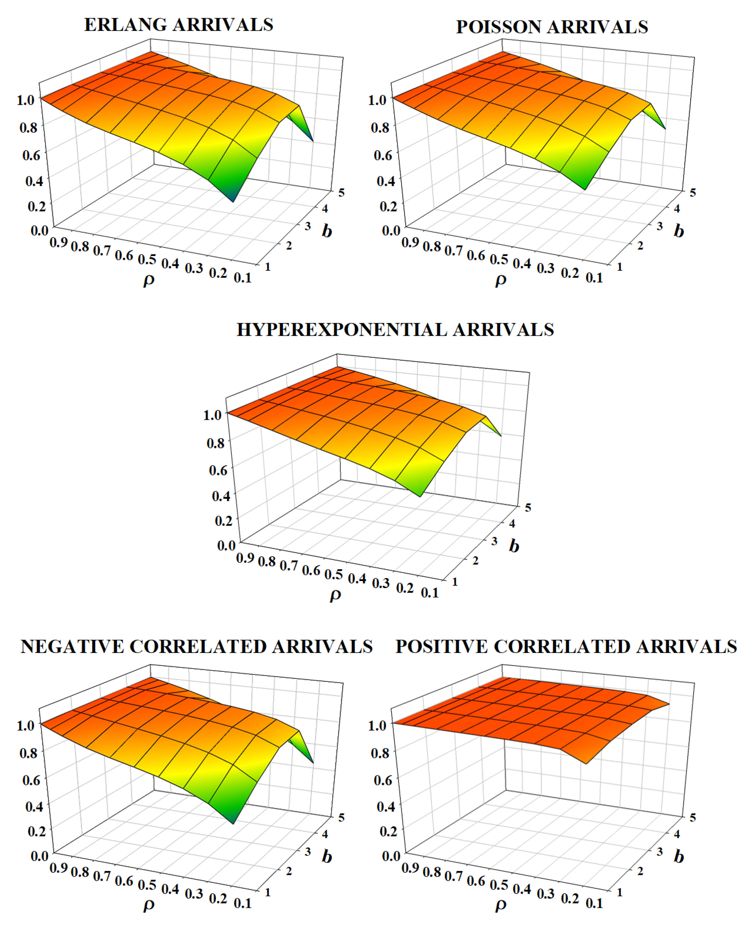
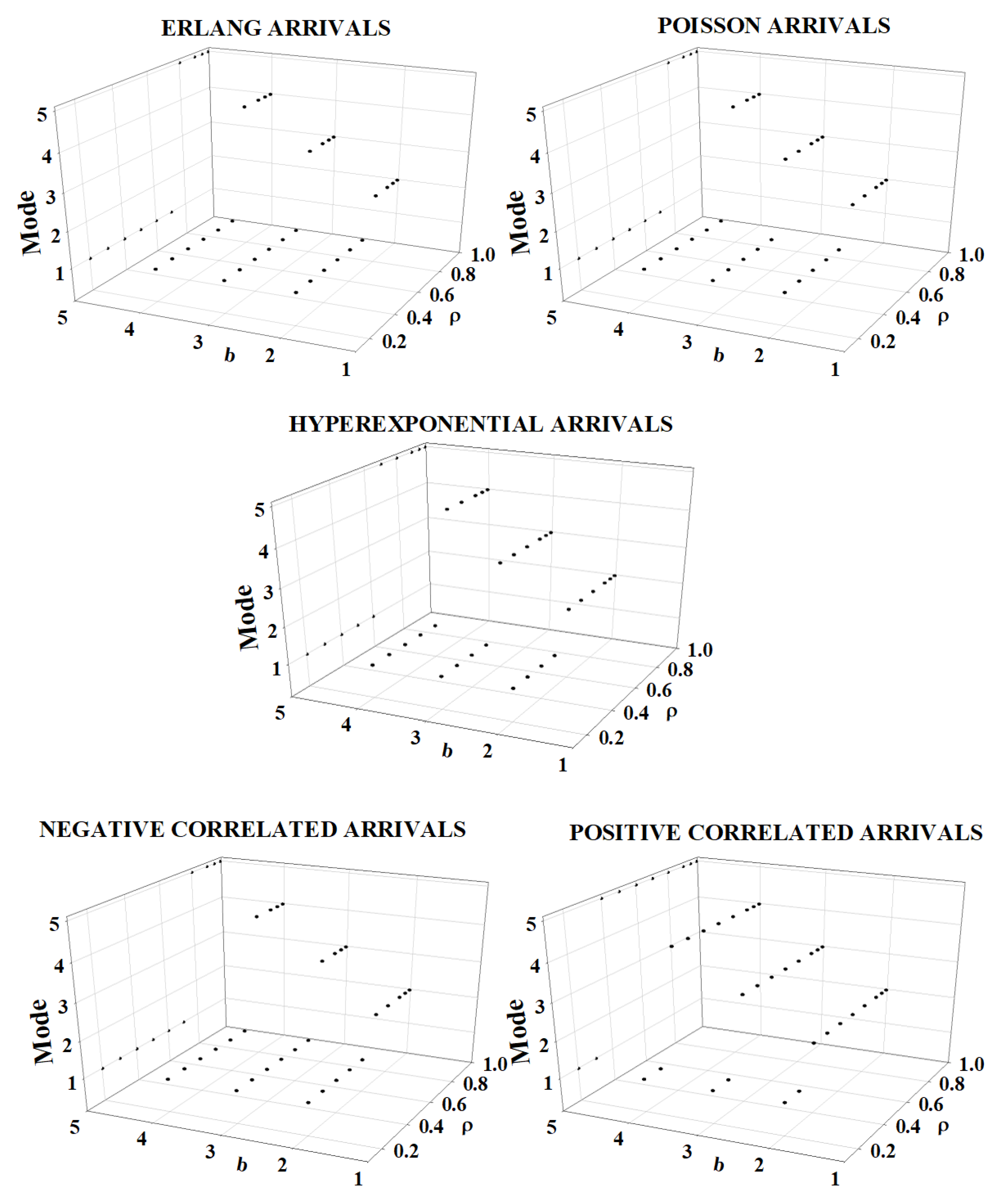
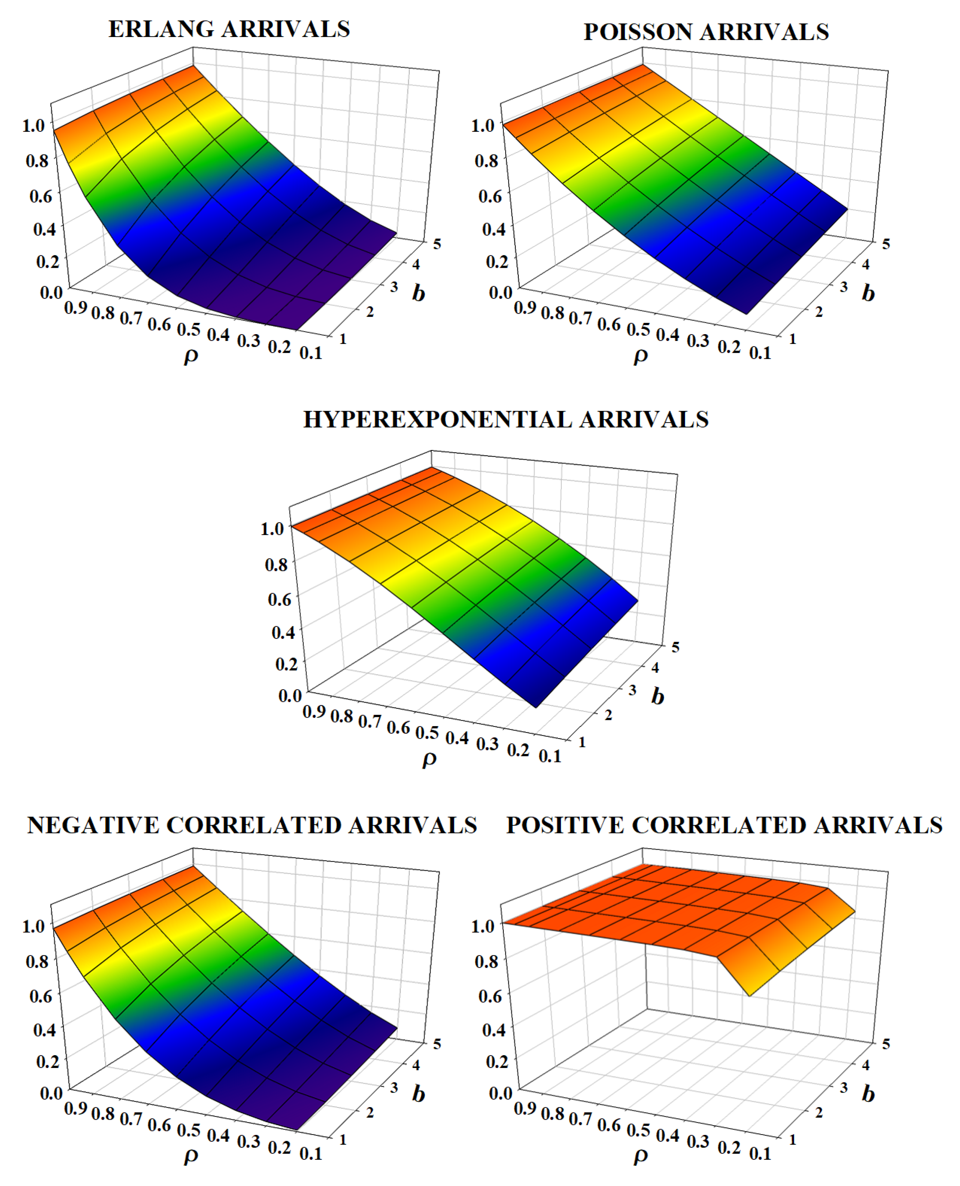
In this example, we look at the five $MAPs$ mentioned above as input to the system where the server can offer services to batches of size up to five customers. The service time for a batch of size r is taken to be $E{R}_r$, for $1\le r\le 5$, as listed above. We vary ρ from 0.2 to 0.99. The plots of ${\mu }_{NiS}$, ${\mu }_{N_q}$, ${\mu }_I^{\prime }$, ${\mu }_{RT}^{\prime }$, and η are displayed in Figure 1, Figure 2, Figure 3, Figure 4 and Figure 5, respectively, under various scenarios. In Figure 6, we display the scatter plot of the mode of the $PMF$ of the number in service. A brief summary of key observations from these figures follows.

1.

The measures ${\mu }_{NiS}$ and ${\mu }_{N_q}$, as functions of b when $\rho$ is fixed as well as functions of $\rho$ when b is fixed, appear to be non-decreasing for all arrival processes considered. However, the interesting fact is when $\rho$ is initially increased from 0.2 to 0.5, we see the $PCA$ case produces the largest rate of increase in these two measures, even though the variability in the inter-arrivals times is less than that of the $HEA$. Comparing both $NCA$ and $PCA$ cases, it is clear that the positively correlated arrivals tend to yield a large value for ${\mu }_{NiS}$.

2.

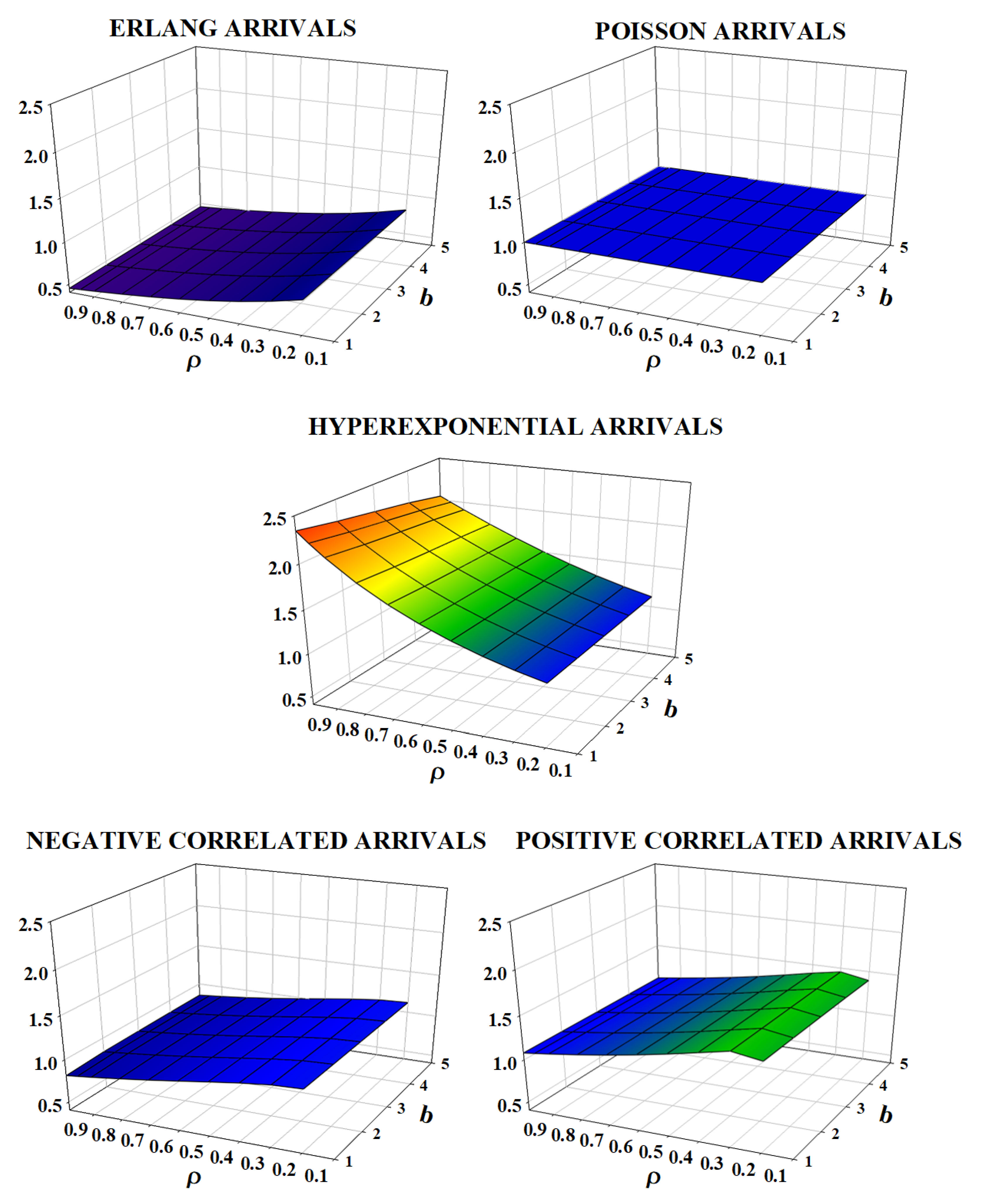
In the case of all arrivals, we notice that the measure, ${\mu }_I^{\prime }$, is not significantly affected by the values of b. However, when $\rho$ is varied (for fixed b), we see an interesting pattern based on the type of arrival processes. In the case of $ERA$ and $NCA$ arrivals, we see that ${\mu }_I^{\prime }$ decreases as $\rho$ is increased. In the case of Poisson ($EXA$) arrivals, it is constant as it should be. For $HEA$, we see this measure increases as $\rho$ is increased, and for the $PCA$ case, the measure initially increases and then decreases as $\rho$ is increased. The increasing phenomenon is somewhat counter-intuitive, but we note that fixing $\rho$ and modifying the service rates accordingly might explain this, especially when the inter-arrival times have a large variability.

3.

Looking at ${\mu }_{RT}^{\prime }$, the plots show the anticipated behavior of an increasing trend when $\rho$ is increased in all cases. It is worth pointing out (not seen from the 3D plot displayed here but from the data) that (a) both $HEA$ and $PCA$ processes dominate the other three under all scenarios; and (b) when comparing $HEA$ and $PCA$ arrivals, we notice that for initial values of $\rho$ (up to around 0.4 to 0.5), the $PCA$ dominates with a large value over $HEA$, and then, the roles are reversed in that $HEA$ dominates $PCA$. This indicates not only the variability but also that the 1-lag (positive) correlation plays a key role.

4.

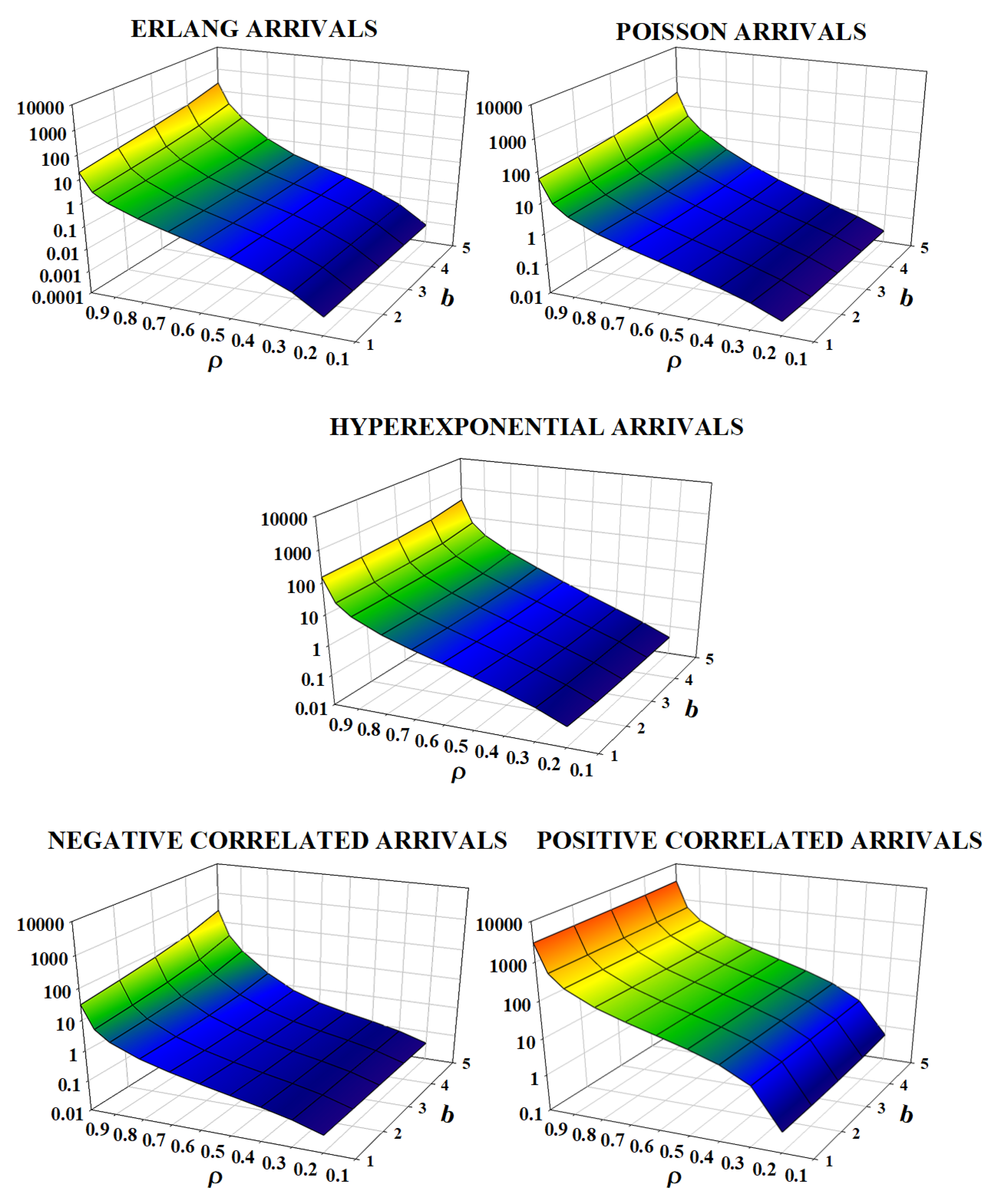
The spectral radius, $\eta$, of the rate matrix indicates an interesting behavior under various scenarios. First, we notice that both $ERA$ and $NCA$ arrivals indicate similar patterns: low values of $\rho$ yielding low values for $\eta$ for b up to 3. However, for other values of b, $\eta$ appears to have reasonably moderate values, indicating that the queue lengths probably stay at moderate values for significant times, and it takes significant times to clear. For Poisson arrivals, it is known that $\rho =\eta$ when $b=1$, and this is also confirmed in the 3D plot. However, as expected, the linearity slowly becomes nonlinear as b is increased. As in the $ERA$ and $NCA$ cases, we do notice some moderate upsurges in the queue lengths when b is close to 5. In the case of $HEA$ arrivals, we see significant upsurges in the queue lengths when $\rho$ is moderately large to large (i.e., 0.9 to 0.99) and for all values of b considered. When looking at $PCA$ arrivals, we see the queue lengths show significant upsurges starting with even low values of $\rho$ (i.e., $\rho >0.2$) and for all values of b. Even though the standard deviation of the inter-arrival times for this $MAP$ is smaller than that of the $HEA$, the values of $\eta$ indicate the significant role played by the 1-lag positive correlation.

5.

We see an interesting pattern for the mode of the $PMF$ of the number of customers in service. First, note that there is nothing to plot when $b=1$. Secondly, under all scenarios, the mode occurs at extreme points, 1 or b. However, the transition point (from 1 to b) depends on the type of the arrival process as well as the traffic intensity, $\rho$. While for $ERA,EXA,$ and $NCA$, the transition point is close to moderate to large values of $\rho$ (for example, in the case of $ERA$, the traffic intensity has to be greater than 0.8 for all $b=2,3,4,5$, whereas for the $HEA$, $\rho$ has to be more than 0.5; and for $PCA$, the values of $\rho$ need to just be more than 0.1). In summary, we see that for the arrival process with either a large variability or with a positive correlation, the server seems to be busy with the maximum batch size even for low to moderate traffic intensity.

Example 2.

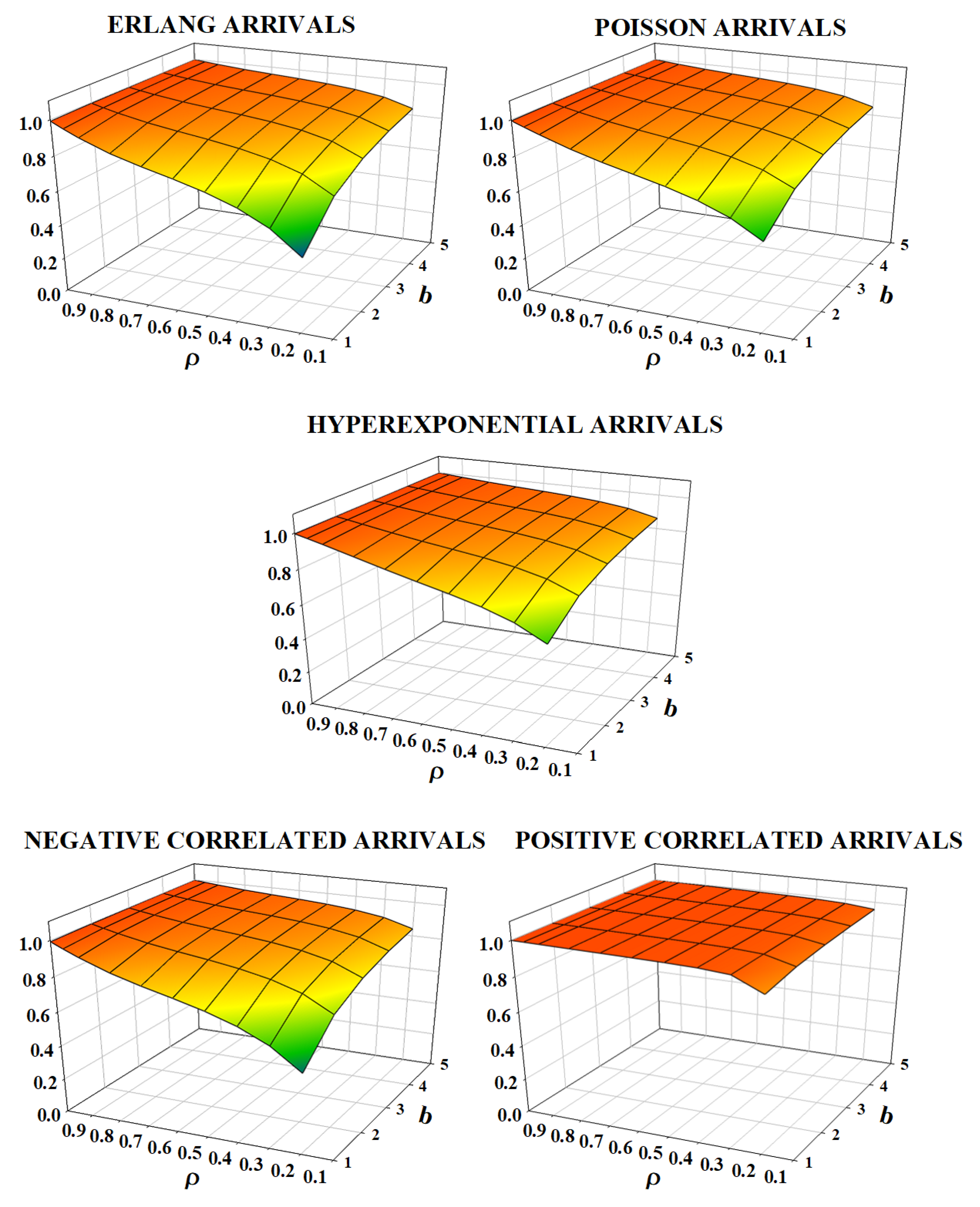
In this example, we look at the five $MAPs$ as input to the system where the server can offer services to batches of size up to five customers. The service time for a batch of size r is taken to be $H{E}_r$, for $1\le r\le 5$, as listed above. We vary ρ from 0.2 to 0.99. The plots of ${\mu }_{NiS}$, ${\mu }_{N_q}$, ${\mu }_I^{\prime }$, ${\mu }_{RT}^{\prime }$, and η are displayed in Figure 7, Figure 8, Figure 9, Figure 10 and Figure 11, respectively, under various scenarios. In Figure 12, we display the scatter plot of the mode of the $PMF$ of the number in service. A brief summary of key observations from these figures follows.

1.

Most of the observations related to the measures ${\mu }_{NiS}$, ${\mu }_{N_q}$, ${\mu }_I^{\prime }$, and ${\mu }_{RT}^{\prime }$ established in Example 1 hold good here but of course with different values for these measures. So, we will only list additional points related to the current example.

2.

For all except $PCA$ arrivals, we notice that ${\mu }_{N_q}$ decreases from $b=4$ to $b=5$ under all scenarios. This is due to having a large variability in services (such as hyperexponential here as compared to Erlang services in Example 1) that probably clears the queue faster frequently and once in a while takes a longer time to process a batch, resulting in this behavior.

3.

The caudal characteristic curve here shows a different behavior for all but $PCA$ arrivals. For $PCA$ arrivals, we noticed in Example 1 significant upsurges in the queue lengths even for Erlang services, and so here with hyperexponential services, one would expect similar upsurges. In the case of all other arrival processes, we see the plot indicates moderate to large upsurges in the queue lengths. Furthermore, we see that $\eta$ increases (for fixed $\rho$) as b increases initially and then $\eta$ decreases. This further explains the same phenomenon seen in ${\mu }_{N_q}$.

4.

The interesting pattern for the mode of the $PMF$ of the number of customers in service is similar to the one discussed in the previous example except that the transition point occurs at or earlier than values of $\rho$ for almost all arrivals.

Example 3.

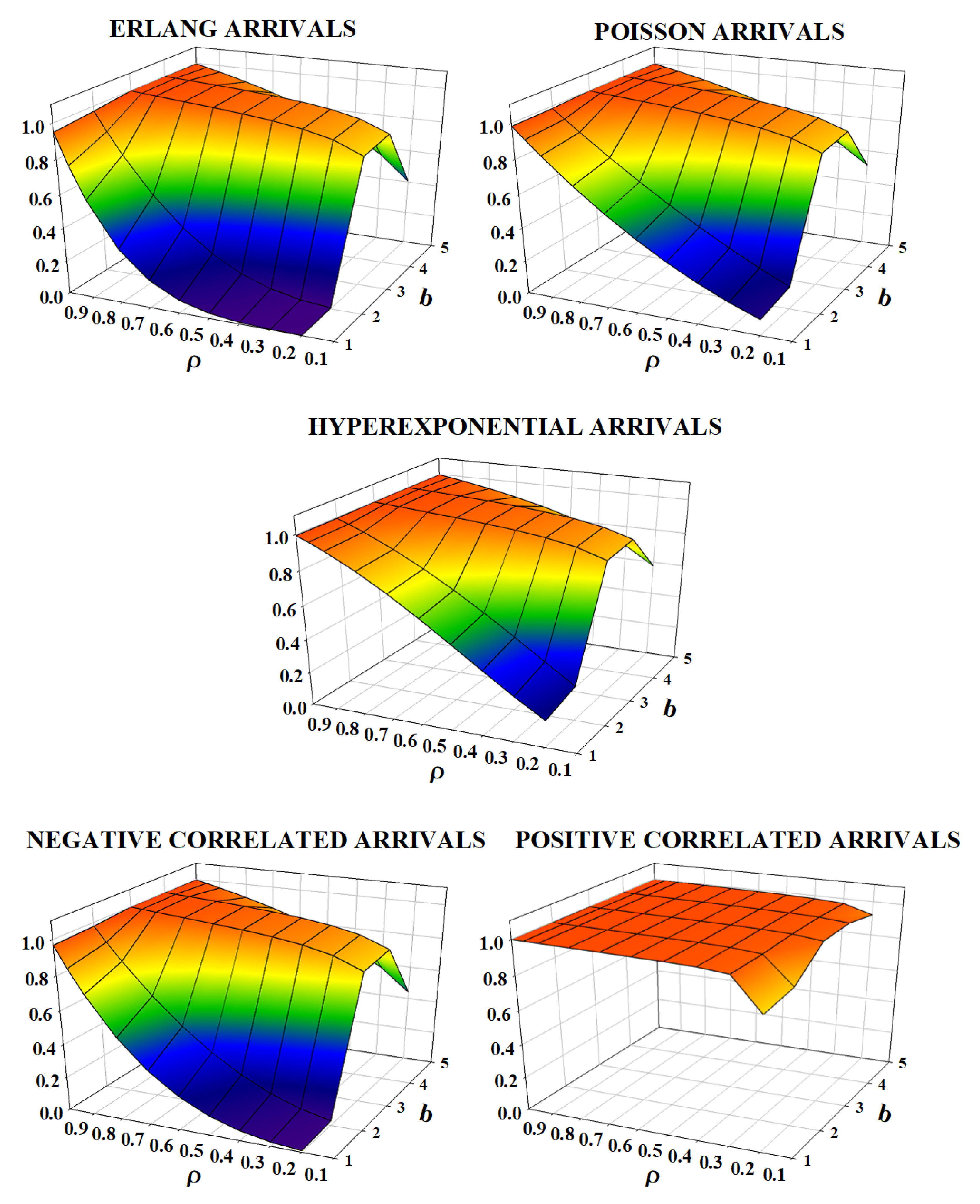
In this example, we look at the five $MAPs$ as input to the system where the server can offer services to batches of size up to five customers. The service time for a batch of size $r,1\le r\le b,$ is taken to be $E{R}_1$, as listed above. That is, we take the same representation for all batch sizes but with varying rates. We vary ρ from 0.2 to 0.99. The measures, ${\mu }_{NiS}$, ${\mu }_{N_q}$, ${\mu }_I^{\prime }$, and ${\mu }_{RT}^{\prime }$ behave similar to the ones discussed in Example 1 except for the values. However, the caudal characteristic curve shows a different behavior. The plot of the measure η is displayed in Figure 13. Compared to Example 1, here, we do not see upsurges in the queue lengths for $ERA,EXA,HEA,$ and $NCA$ cases. However, for $PCA$ the upsurges are similar.

Example 4.

In this example, we look at the five $MAPs$ as input to the system where the server can offer services to batches of size up to five customers. The service time for a batch of size r is taken to be $H{E}_1$, as listed above. That is, we take the same representation for all batch sizes but with varying rates. We vary ρ from 0.2 to 0.99. The measures, ${\mu }_{NiS}$, ${\mu }_{N_q}$, ${\mu }_I^{\prime }$, and ${\mu }_{RT}^{\prime }$ behave similar to the ones discussed in Example 3 except for the values. However, the caudal characteristic curve shows a different behavior. The plot of the measure η is displayed in Figure 14. Compared to Example 3, here, we do see significant upsurges in the queue lengths, especially for $b\ge 2$, for all arrivals. In the $PCA$ case, even for $b=1$, we notice significant upsurges. This again shows that a large variability in the services will lead to the queue lengths exhibiting a large value and takes a long duration to clear.

Example 5.

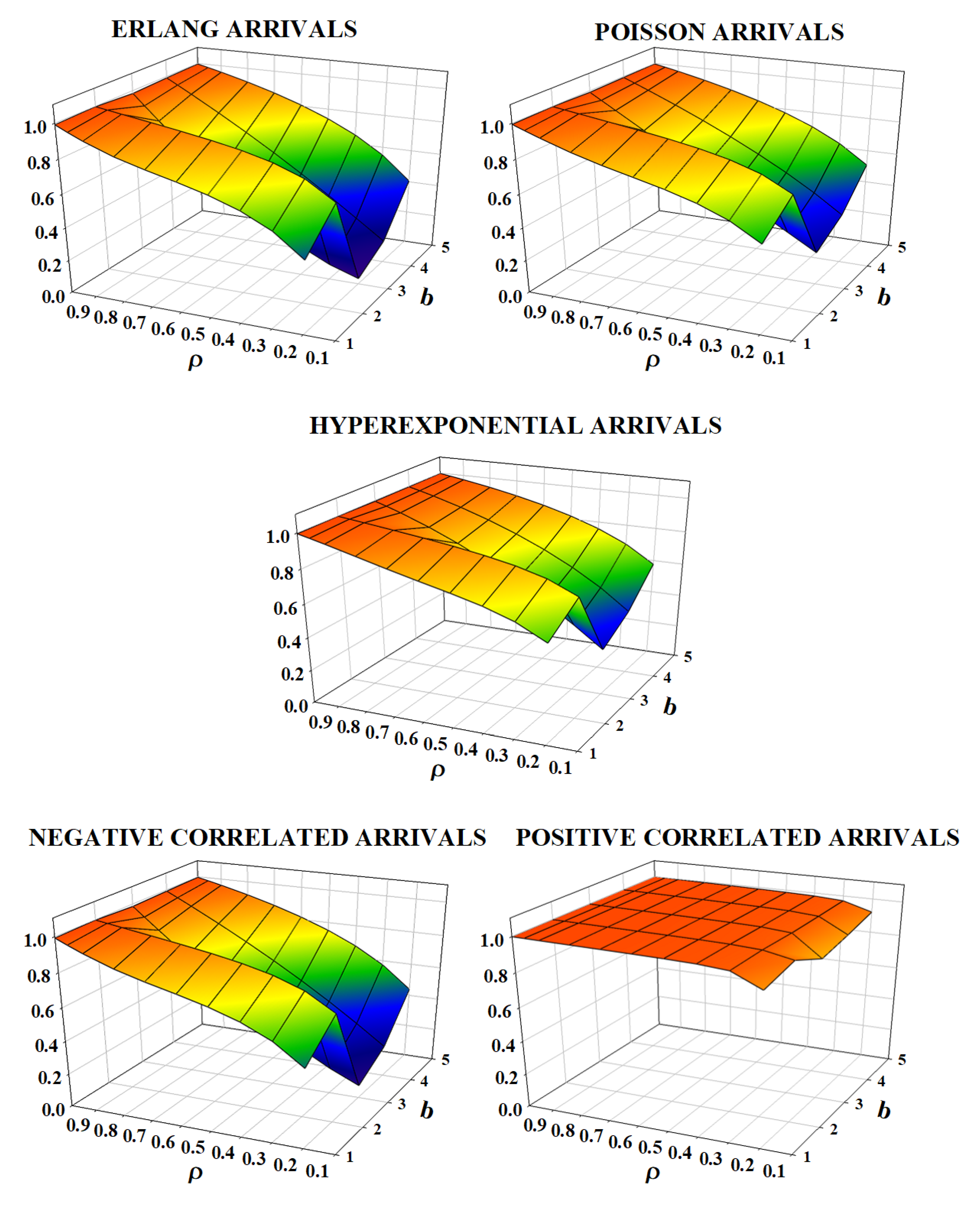
In this example, we look at the five $MAPs$ as input to the system where the server can offer services to batches of size up to five customers. The service time for a batch of size $r,1\le r\le 2$, is taken to be $E{R}_1$ and $E{R}_2$, respectively, and for $r,3\le r\le 5$, it is taken to be $H{E}_3,H{E}_4,$ and $H{E}_5$, respectively. The purpose of this choice of the service time distribution is to see how a combination of Erlangs for $b=1,2$, and hyperexponentials for the other values of b, will affect the spectral radius of the rate matrix R. We vary ρ from 0.2 to 0.99. The plot of the measure η is displayed in Figure 15. Compared to Examples 1 and 2, here, we do see some interesting patterns for all but $PCA$ arrivals. We notice an increasing/decreasing trend in this measure as b is increased. For the $PCA$ arrivals, the pattern is similar to the earlier examples.

Example 6.

In this example, we look at the five $MAPs$ as input to the system where the server can offer services to batches of size up to five customers. The service time for a batch of size $r,1\le r\le 2$, is taken to be $H{E}_1$ and $H{E}_2$, respectively, and for $r,3\le r\le 5$, it is taken to be $E{R}_3,E{R}_4,$ and $E{R}_5$, respectively. The purpose of this choice of the service time distribution is to see how a combination of hyperexponentials for $b=1,2$, and Erlangs for the other values of b, will affect the spectral radius of the rate matrix R. We vary ρ from 0.2 to 0.99. The plot of the measure η is displayed in Figure 16. Compared to Examples 1 and 2, here, we do see some interesting patterns for all but $PCA$ arrivals. We notice an increasing/decreasing/increasing trend in this measure as b is increased. For the $PCA$ arrivals, the pattern is similar to the earlier examples.

5. Conclusions

In this paper, we considered a queueing model in which arrivals occur according to a Markovian arrival process and the services are offered in batches of varying sizes. The service times are modeled using phase-type distributions with representations depending on the number served in a batch. Illustrative numerical examples point out that having a large variability or a 1-lag positive correlation in the inter-arrival times results in the queue lengths exhibiting upsurges. Furthermore, if the service times have a significant variability, the upsurges in the queue lengths appear to occur even when the inter-arrival times have a small variability such as the Erlang distribution. The model studied here can be extended to include $BMAP$ arrivals, which is currently being investigated.

References

- Neuts, M.F. A general class of bulk queues with Poisson input. Ann. Math. Stat. 1967, 38, 759–770. [Google Scholar] [CrossRef]
- Banerjee, A.; Gupta, U.; Chakravarthy, S. Analysis of a finite-buffer bulk-service queue under Markovian arrival process with batch-size-dependent service. Comput. Oper. Res. 2015, 60, 138–149. [Google Scholar] [CrossRef]
- Brugno, A.; D’Apice, C.; Dudin, A.; Manzo, R. Analysis of an MAP/PH/1 Queue with Flexible Group Service. Int. J. Appl. Math. Comput. Sci. 2017, 27, 119–131. [Google Scholar] [CrossRef]
- Brugno, A.; Dudin, A.; Manzo, R. Retrial queue with discipline of adaptive permanent pooling. Appl. Math. Model. 2017, 50, 1–16. [Google Scholar] [CrossRef]
- Chakravarthy, S.R.; Maity, A.; Gupta, U.C. An ‘(s, S)’inventory in a queueing system with batch service facility. Ann. Oper. Res. 2017, 258, 263–283. [Google Scholar] [CrossRef]
- Chaudhry, M.L.; Templeton, J.G.C. A First Course in Bulk Queues; John Wiley & Sons: New York, NY, USA, 1983. [Google Scholar]
- D’Arienzo, M.P.; Dudin, A.N.; Dudin, S.A.; Manzo, R. Analysis of a retrial queue with group service of impatient customers. J. Ambient. Intell. Humaniz. Comput. 2020, 11, 2591–2599. [Google Scholar] [CrossRef]
- Dudin, A.N.; Manzo, R.; Piscopo, R. Single server retrial queue with group admission of customers. Comput. Oper. Res. 2020, 61, 89–99. [Google Scholar] [CrossRef]
- Baba, Y. A bulk service gi/m/1 queue with service rates depending on service batch size. J. Oper. Res. Soc. Jpn. 1996, 39, 25–35. [Google Scholar] [CrossRef]
- Chakravarthy, S. Introduction to Matrix-Analytic Methods in Queues 1: Analytical and Simulation Approach—Basics; ISTE Ltd.: London, UK; John Wiley and Sons: New York, NY, USA, 2022. [Google Scholar]
- Bladt, M.; Nielsen, B.F. Matrix-Exponential Distributions in Applied Probability; Springer: New York, NY, USA, 2017. [Google Scholar]
- He, Q.-M. Fundamentals of Matrix-Analytic Methods; Springer: New York, NY, USA, 2014. [Google Scholar]
- Neuts, M.F. Matrix-Geometric Solutions in Stochastic Models—An Algorithmic Approach; Dover Publications: Mineola, NY, USA, 1995. [Google Scholar]
- Chakravarthy, S.R.; Rumyantsev, A. Efficient redundancy techniques in cloud and desktop grid systems using MAP/G/c-type queues. Open Eng. 2018, 8, 17–31. [Google Scholar] [CrossRef]
- Dudin, A.N.; Klimenok, V.I.; Vishnevsky, V.M. The Theory of Queuing Systems With Correlated Flows; Springer: Berlin/Heidelberg, Germany, 2019. [Google Scholar]
- Chakravarthy, S.R. The Batch Markovian Arrival Process: A Review and Future Work. In Advances in Probability Theory and Stochastic Processes; Krishnamoorthy, A., Raju, N., Ramaswami, V., Eds.; Notable Publications, Inc.: Woodland Park, NJ, USA, 2001; pp. 21–49. [Google Scholar]
- Lucantoni, D.; Meier-Hellstern, K.S.; Neuts, M.F. A single-server queue with server vacations and a class of nonrenewal arrival processes. Adv. Appl. Probab. 1990, 22, 676–705. [Google Scholar] [CrossRef]
- Lucantoni, D. New results on the single server queue with a batch Markovian arrival process. Stoch. Model. 1991, 7, 1–46. [Google Scholar] [CrossRef]
- Neuts, M.F. A versatile Markovian point process. J. Appl. Probab. 1979, 16, 764–779. [Google Scholar] [CrossRef]
- Chakravarthy, S.R. Markovian Arrival Processes. In Wiley Encyclopedia of Operations Research and Management Science; Wiley: Hoboken, NJ, USA, 2010. [Google Scholar]
- Neuts, M.F. Structured Stochastic Matrices of M/G/1 Type and Their Applications; Marcel Dekker: New York, NY, USA, 1989. [Google Scholar]
- Neuts, M.F. Models based on the Markovian arrival processes. IEICE Trans. Commun. 1992, E75-B, 1255–1265. [Google Scholar]
- Neuts, M.F. Probability distributions of phase type. In Liber Amicorum Prof. Emeritus H. Florin; Department of Mathematics, University of Louvain: Ottignies-Louvain-la-Neuve, Belgium, 1975; pp. 173–206. [Google Scholar]
- Chakravarthy, S. Introduction to Matrix-Analytic Methods in Queues 2: Analytical and Simulation Approach—Queues and Simulation; ISTE Ltd.: London, UK; John Wiley and Sons: New York, NY, USA, 2022. [Google Scholar]
- Latouche, G.; Ramaswami, V. Introduction to Matrix Analytic Methods in Stochastic Modeling; SIAM: Philadelphia, PA, USA, 1999. [Google Scholar]
- Neuts, M.F. The caudal characteristic curve of queus. Adv. Appl. Probab. 1986, 18, 221–254. [Google Scholar] [CrossRef]
Figure 1.
Conditional mean number in service () for example 1.
Figure 2.
Mean number in queue () for example 1.
Figure 3.
Mean idle time () for example 1.
Figure 4.
Mean recurrence time () for example 1.
Figure 5.
Spectral radius () of the matrix R for example 1.
Figure 6.
Scatter plot of the mode of the conditional of the number in service for example 1.
Figure 7.
Conditional mean number in service () for example 2.
Figure 8.
Mean number in queue () for example 2.
Figure 9.
Mean idle time () for example 2.
Figure 10.
Mean recurrence time () for example 2.
Figure 11.
Spectral radius () of the matrix R for example 2.
Figure 12.
Scatter plot of the mode of the of number in service for example 1.
Figure 13.
Spectral radius () for example 3.
Figure 14.
Spectral radius () for example 4.
Figure 15.
Spectral radius () for example 5.
Figure 16.
Spectral radius () for example 6.
Publisher’s Note: MDPI stays neutral with regard to jurisdictional claims in published maps and institutional affiliations. |
© 2022 by the author. Licensee MDPI, Basel, Switzerland. This article is an open access article distributed under the terms and conditions of the Creative Commons Attribution (CC BY) license (https://creativecommons.org/licenses/by/4.0/).
Share and Cite
MDPI and ACS Style
Chakravarthy, S.R. Analysis of a Queueing Model with MAP Arrivals and Heterogeneous Phase-Type Group Services. Mathematics 2022, 10, 3575. https://0-doi-org.brum.beds.ac.uk/10.3390/math10193575
AMA Style
Chakravarthy SR. Analysis of a Queueing Model with MAP Arrivals and Heterogeneous Phase-Type Group Services. Mathematics. 2022; 10(19):3575. https://0-doi-org.brum.beds.ac.uk/10.3390/math10193575
Chicago/Turabian StyleChakravarthy, Srinivas R. 2022. "Analysis of a Queueing Model with MAP Arrivals and Heterogeneous Phase-Type Group Services" Mathematics 10, no. 19: 3575. https://0-doi-org.brum.beds.ac.uk/10.3390/math10193575
Note that from the first issue of 2016, this journal uses article numbers instead of page numbers. See further details here.